Tensor Networks for Big Data Analytics and Large-Scale Optimization Problems

Andrzej CICHOCKI
RIKEN Brain Science Institute, Japan
and Systems Research Institute of the Polish Academy of Science, Poland
Part of this work was presented on the Second International Conference on Engineering and Computational Mathematics (ECM2013), Hong Kong December 16-18, 2013 (invited talk)
Abstract

Tensor decompositions and tensor networks are emerging and promising tools for data analysis and data mining. In this paper we review basic and emerging models and associated algorithms for large-scale tensor networks, especially Tensor Train (TT) decompositions using novel mathematical and graphical representations. We discus the concept of tensorization (i.e., creating very high-order tensors from lower-order original data) and super compression of data achieved via quantized tensor train (QTT) networks. The main objective of this paper is to show how tensor networks can be used to solve a wide class of big data optimization problems (that are far from tractable by classical numerical methods) by applying tensorization and performing all operations using relatively small size matrices and tensors and applying iteratively optimized and approximative tensor contractions.

Keywords: Tensor networks, tensor train (TT) decompositions, matrix product states (MPS), matrix product operators (MPO), basic tensor operations, optimization problems for very large-scale problems: generalized eigenvalue decomposition (GEVD), PCA/SVD, canonical correlation analysis (CCA).

I Introduction and Motivations
Refer to caption
Refer to caption
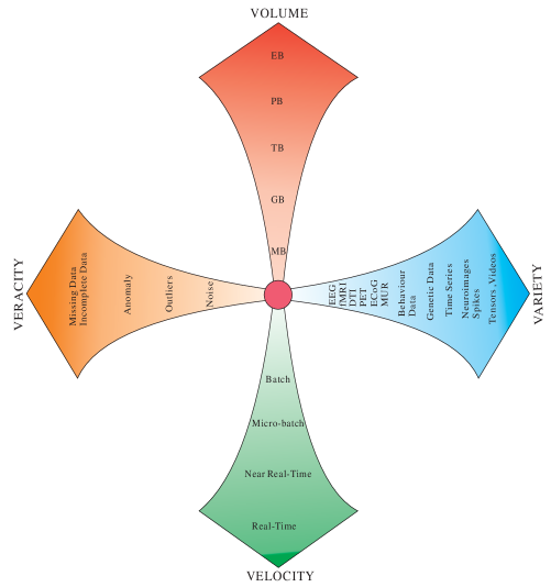
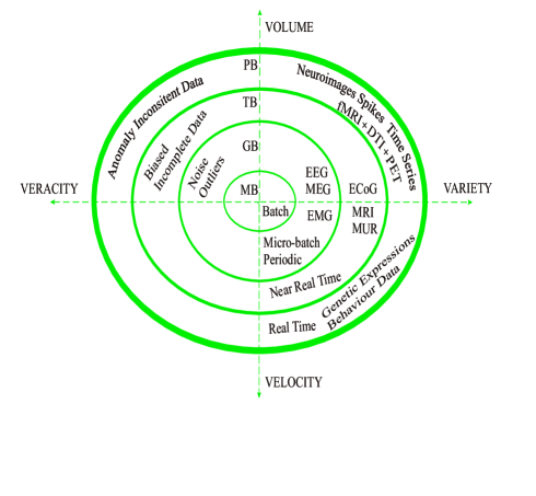
Figure  1: Four “V”s of big (brain) data: Volume - scale of data, Variety - different forms (types) of data, Veracity - uncertainty of data, and Velocity - speed at which stream of data is generated and processed. Illustration of challenges for human brain data, which involves analysis of multi-modal, multi-subjects neuroimages, spectrograms, time series, spikes trains, genetic and behavior data. One of the challenges in computational and system neuroscience is to perform fusion or assimilation for various kinds of data and to understand the relationship and links between them. Brain data can be recorded by electroencephalography (EEG), electrocorticography (ECoG), magnetoencephalography (MEG), fMRI, DTI, PET, Multi Unit Recording (MUR), to name a few.

Big Data can have a such huge volume and high complexity that existing standard methods and algorithms become inadequate for the processing and optimization of such data. Big data is characterized not only by big Volume but also by other specific “V” features/challenges: Veracity, Variety, Velocity, Value. Fig. 1 illuminates the big data characteristics for brain research related problems. High Volume implies the need for algorithms that are scalable; high Velocity is related to the processing of stream of data in near real-time; high Veracity calls for robust and predictive algorithms for noisy, incomplete and/or inconsistent data, high Variety require integration across different types of data, e.g., binary, continuous data, images, time series, etc., and finally Value refers to extracting high quality and consistent data which could lend themselves to meaningful and interpretable results.

Multidimensional data is becoming ubiquitous across the sciences and engineering because they are increasingly being gathered by information-sensing devices and remote sensing. Big data such as multimedia data (speech, video), and medical/biological data, the analysis of which critically requires a paradigm shift in order to efficiently process massive datasets within tolerable time. Tensors – multi-dimensional generalizations of matrices, provide often a natural sparse and distributed representation for such data.

Tensors have been adopted in diverse branches of data analysis, such as in signal and image processing, Psychometric, Chemometrics, Biometric, Quantum Physics/Information, Quantum Chemistry and Brain Science [1, 2, 3, 4, 5, 6, 7, 8]. Tensors are particularly attractive for data which exhibit not only huge volumes but also very high variety, for example, they are suited for problems in bio- and neuro-informatics or computational neuroscience where data are collected in various forms of big, sparse tabular, graphs or networks with multiple aspects and high dimensionality.

Tensor decompositions (TDs) provide some extensions of blind source separation (BSS) and 2-way (matrix) Component Analysis (2-way CA) to multi-way component analysis (MWCA) methods [1]. Furthermore, TNs/TDs are suitable for dimensionality reduction, they can handle missing values, and noisy data [9]. They are also potentially useful for analysis of linked (coupled) block of big tensors with millions and even billions of non-zero entries, using the map-reduce paradigm, as well as out-of-core approaches [2, 10, 11, 12, 13]. Moreover, multi-block tensors which arise in numerous important applications (that require the analysis of diverse and partially related data) can be decomposed to common (or correlated) and uncorrelated or statistically independent components. The effective analysis of coupled tensors requires the development of new models and associated algorithms and software that can identify the core relations that may exist among the different tensors, and scale to extremely large datasets.

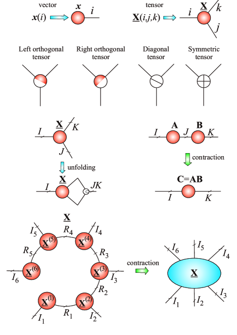
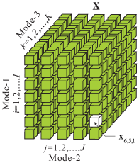
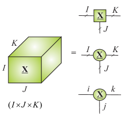
Complex interactions and operations between tensors can be visualized by tensor network diagrams in which tensors are represented graphically by nodes or any shapes (e.g., circles, spheres, triangular, squares, ellipses) and each outgoing edge (line) emerging from a node represents a mode (a way, a dimension, indices) (see Fig. 2). In contrast to classical graphs, in tensor network diagrams an edge does not need connect two nodes, but may be connected to only one node. Each such free (dangling) edge corresponds to a (physical) mode that is not contracted and, hence, the order of the entire tensor network is given by the number of free (dangling) edges (see Fig. 3). Tensor network diagrams are very helpful not only in visualizing tensor decompositions but also to express complex mathematical (multilinear) operations of contractions of tensors. Tensor networks are connected to quantum physics, quantum chemistry and quantum information, which studies the ways to possibly build a quantum computer and to program it [14, 15].
Refer to caption
Refer to caption
Figure  2: A 3rd-order tensor 𝐗¯I×J×K¯𝐗superscript𝐼𝐽𝐾\underline{{\bf X}}\in\mathbb{R}^{I\times J\times K} with entries xijk=𝐗¯(i,j,k)subscript𝑥𝑖𝑗𝑘¯𝐗𝑖𝑗𝑘x_{ijk}=\underline{{\bf X}}(i,j,k) and exemplary symbols used in tensor network diagrams. Each node in the diagram represents a tensor and each edge represents a mode or dimension. We indicate maximum size in each mode by I,J,K𝐼𝐽𝐾I,J,K or running indices: i=1,2,,I;j=1,2,,Jformulae-sequence𝑖12𝐼𝑗12𝐽i=1,2,\ldots,I;\;j=1,2,\ldots,J and k=1,2,,K𝑘12𝐾k=1,2,\ldots,K.
Refer to caption
Figure  3: Basic symbols and operations for tensor network diagrams. Modes (dimensions) are indicated by running indices (i,j,k,𝑖𝑗𝑘i,j,k,\ldots where i=1,2,,I𝑖12𝐼i=1,2,\ldots,I;   j=1,2,,J𝑗12𝐽j=1,2,\ldots,J;   k=1,2,,K𝑘12𝐾k=1,2,\ldots,K, r=1,2,,R𝑟12𝑅r=1,2,\ldots,R) in each mode or size of the modes (I,J,K,R𝐼𝐽𝐾𝑅I,J,K,R\ldots). For higher order tensors we will use the symbol in=1,2,,Insubscript𝑖𝑛12subscript𝐼𝑛i_{n}=1,2,\ldots,I_{n} for n=1,2,,N𝑛12𝑁n=1,2,\ldots,N, where N𝑁N is the order of a tensor. The minimum set of internal indices {R1,R2,R3,}subscript𝑅1subscript𝑅2subscript𝑅3\{R_{1},R_{2},R_{3},\ldots\} is called the multilinear rank od a specific tensor network [14].

To summarize, the benefits of multiway (tensor) analysis methods for big data include:

  • “Super” - compression of huge multidimensional data via tensorization and decompositions of a high-order tensor into factor matrices and/or core tensors of low-rank and low-order;

  • By performing all mathematical operations in feasible tensor formats [16];

  • Very flexible distributed representations of structurally rich data;

  • Possibility to operate with noisy and missing data by using powerful low-rank tensor/matrix approximations and by exploiting robustness and stability of tensor network decomposition algorithms;

  • A framework to incorporate various diversities or constraints in different modes or different factors (core tensors) and thus naturally extend the standard (2-way) CA and BSS methods to large-scale multidimensional data;

  • Tensor networks not only provide graphically illustrative large distributed networks but also perform complex tensor operations (i.e., tensor contractions and reshaping) in an intuitive way and without using explicitly mathematical expressions.

Review and tutorial papers [1, 4, 17, 18, 19, 20] and books [7, 8, 3, 6] dealing with TDs and TNs already exist, however, they typically focus on standard models and/or do not provide explicit links to big data processing topics and/or do not explore connections to wide class of optimization problems. This paper extends beyond the standard tensor decomposition models such as the Tucker and CPD models, and aims to demonstrate flexibilities of TNs in the optimization problems of multi-dimensional, multi-modal data, together with their role as a mathematical backbone for the discovery of hidden structures in large-scale data [3, 4].

5th-order tensor
Refer to caption
6th-order tensor
Refer to caption

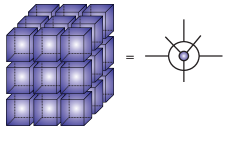
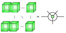
Figure  4: Symbols and graphical representations of higher-order block tensors. Outer circle indicates global structure of a block tensor (e.g., matrix, a 3rd-order tensor), while inner circle indicate the structure of each element or block of the tensor.

Our objective is to both review tensor models for big data, and to systematically introduce emerging models and associated algorithms for large-scale TNs/TDs, together with illustrating the many potential applications. Apart from the optimization framework considered many other challenging problems for big data related to anomaly detection, visualization, clustering, feature extraction and classification can also be solved using tensor network decompositions and low-rank tensor approximations.

II Basic Tensor Operations

A higher-order tensor can be interpreted as a multiway array of numbers, as illustrated in Figs. 2 and 3. Tensors are denoted by bold underlined capital letters, e.g., 𝐗¯I1×I2××IN¯𝐗superscriptsubscript𝐼1subscript𝐼2subscript𝐼𝑁\underline{{\bf X}}\in\mathbb{R}^{I_{1}\times I_{2}\times\cdots\times I_{N}} (we assume we shall assume that all entries of a tensor are real-valued). The order of a tensor is the number of its “modes”, “ways” or “dimensions”, which include e.g., space, time, frequency, trials, classes, and dictionaries. Matrices (2nd-order tensors) are denoted by boldface capital letters, e.g., 𝐗𝐗{\bf X}, and vectors (1st-order tensors) by boldface lowercase letters; for instance the columns of the matrix 𝐀=[𝒂1,𝒂2,,𝒂R]I×R𝐀subscript𝒂1subscript𝒂2subscript𝒂𝑅superscript𝐼𝑅{\bf A}=[\mbox{\boldmath$a$}_{1},\mbox{\boldmath$a$}_{2},\ldots,\mbox{\boldmath$a$}_{R}]\in\mathbb{R}^{I\times R} are denoted by 𝒂rsubscript𝒂𝑟\mbox{\boldmath$a$}_{r} and elements of a matrix (scalars) are denoted by lowercase letters, e.g., airsubscript𝑎𝑖𝑟a_{ir}. Basic tensor and TN notations are given in Table I and illustrated in Figs. 24. It should be noted that hierarchical block matrices can be represented by tensors and vice versa. For example, 3rd- and 4th-order tensors can be represented by block matrices and all algebraic operations can be equally performed on block matrices [2].

The most common tensor multiplications are denoted by: tensor-product\otimes for the Kronecker, direct-product\odot for the Khatri-Rao, \circledast for the Hadamard (componentwise), \circ for the outer and ×nsubscript𝑛\times_{n} for the mode-n𝑛n products (see also Table I). General basic operations, e.g., vec()𝑣𝑒𝑐vec(\cdot), diag{}diag\mathop{\rm diag}\nolimits\{\cdot\}, are defined as in MATLAB. We refer to [2, 3, 4] for more detail regarding the basic notations and tensor operations.

Subtensors are formed when a subset of indices is fixed. Of particular interest are fibers (vectors), defined by fixing every index but one, and slices which are two-dimensional sections (matrices) of a tensor, obtained by fixing all the indices but two. A matrix has two modes: rows and columns, while an N𝑁Nth-order tensor has N𝑁N modes.

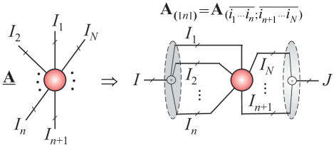
The process of unfolding (see Fig. 5) flattens a tensor into a matrix [4]. In the simplest scenario, mode-n𝑛n unfolding (matricization, flattening) of the tensor 𝐀¯I1×I2××IN¯𝐀superscriptsubscript𝐼1subscript𝐼2subscript𝐼𝑁\underline{{\bf A}}\in\mathbb{R}^{I_{1}\times I_{2}\times\cdots\times I_{N}} yields a matrix 𝐀(n)In×(I1In1In+1IN)subscript𝐀𝑛superscriptsubscript𝐼𝑛subscript𝐼1subscript𝐼𝑛1subscript𝐼𝑛1subscript𝐼𝑁{\bf A}_{(n)}\in\mathbb{R}^{I_{n}\times(I_{1}\cdots I_{n-1}I_{n+1}\cdots I_{N})}, with entries ain,i2,,in1,in+1,,in)a_{i_{n},i_{2},\ldots,i_{n-1},i_{n+1},\ldots,i_{n})} such that grouped indices (i1,,in1,in+1,,iN)subscript𝑖1subscript𝑖𝑛1subscript𝑖𝑛1subscript𝑖𝑁(i_{1},\ldots,i_{n-1},i_{n+1},\ldots,i_{N}) are arranged in a specific order, (in this paper rows and columns are ordered colexicographically). In tensor networks we use, typically a generalized mode-([n])delimited-[]𝑛([n]) unfolding as illustrated in Fig. 5.

Refer to caption
Figure  5: Unfolding the N𝑁Nth-order tensor 𝐀¯I1×I2××IN¯𝐀superscriptsubscript𝐼1subscript𝐼2subscript𝐼𝑁\underline{{\bf A}}\in\mathbb{R}^{I_{1}\times I_{2}\times\cdots\times I_{N}} i̊nto a matrix 𝐀([n])=𝐀(i1in¯;in+1iN¯)I1I2In×In+1INsubscript𝐀delimited-[]𝑛subscript𝐀¯subscript𝑖1subscript𝑖𝑛¯subscript𝑖𝑛1subscript𝑖𝑁superscriptsubscript𝐼1subscript𝐼2subscript𝐼𝑛subscript𝐼𝑛1subscript𝐼𝑁{\bf A}_{([n])}={\bf A}_{(\overline{i_{1}\cdots i_{n}}\;;\;\overline{i_{n+1}\cdots i_{N}})}\in\mathbb{R}^{I_{1}I_{2}\cdots I_{n}\times I_{n+1}\cdots I_{N}}. All entries of an unfolded tensor are arranged in a specific order. In a more general case, let 𝒓={m1,m2,,mR}{1,2,,N}𝒓subscript𝑚1subscript𝑚2subscript𝑚𝑅12𝑁\mbox{\boldmath$r$}=\{m_{1},m_{2},\ldots,m_{R}\}\subset\{1,2,\ldots,N\} be the row indices and 𝒄={n1,n2,,nC}{1,2,,N}𝒓𝒄subscript𝑛1subscript𝑛2subscript𝑛𝐶12𝑁𝒓\mbox{\boldmath$c$}=\{n_{1},n_{2},\ldots,n_{C}\}\subset\{1,2,\ldots,N\}-\mbox{\boldmath$r$} be the column indices, then the mode-(𝒓,𝒄)𝒓𝒄(\mbox{\boldmath$r$},\mbox{\boldmath$c$}) unfolding of 𝐀¯¯𝐀\underline{{\bf A}} is denoted as 𝐀(𝒓,𝒄)Im1Im2ImR×In1In2InCsubscript𝐀𝒓𝒄superscriptsubscript𝐼subscript𝑚1subscript𝐼subscript𝑚2subscript𝐼subscript𝑚𝑅subscript𝐼subscript𝑛1subscript𝐼subscript𝑛2subscript𝐼subscript𝑛𝐶{\bf A}_{(\mbox{\boldmath$r$},\mbox{\boldmath$c$})}\in\mathbb{R}^{I_{m_{1}}I_{m_{2}}\cdots I_{m_{R}}\times I_{n_{1}}I_{n_{2}}\cdots I_{n_{C}}}.
TABLE I: Basic tensor notation and matrix/tensor products.

𝐗¯I1×I2××IN¯𝐗superscriptsubscript𝐼1subscript𝐼2subscript𝐼𝑁\underline{{\bf X}}\in\mathbb{R}^{I_{1}\times I_{2}\times\cdots\times I_{N}} N𝑁Nth-order tensor of size I1×I2××INsubscript𝐼1subscript𝐼2subscript𝐼𝑁I_{1}\times I_{2}\times\cdots\times I_{N} 𝐆¯(n),𝐗¯(n),𝐒¯superscript¯𝐆𝑛superscript¯𝐗𝑛¯𝐒\underline{{\bf G}}^{(n)},\;\underline{{\bf X}}^{(n)},\;\underline{{\bf S}} core tensors 𝚲¯R×R××R¯𝚲superscript𝑅𝑅𝑅\underline{\mbox{\boldmath$\Lambda$}}\in\mathbb{R}^{R\times R\times\cdots\times R} diagonal core tensor with nonzero λrsubscript𝜆𝑟\lambda_{r} entries on diagonal 𝐀=[𝒂1,𝒂2,,𝒂R]I×R𝐀subscript𝒂1subscript𝒂2subscript𝒂𝑅superscript𝐼𝑅{\bf A}=[\mbox{\boldmath$a$}_{1},\mbox{\boldmath$a$}_{2},\ldots,\mbox{\boldmath$a$}_{R}]\in\mathbb{R}^{I\times R} matrix with column vectors 𝒂rIsubscript𝒂𝑟superscript𝐼\mbox{\boldmath$a$}_{r}\in\mathbb{R}^{I} and entries airsubscript𝑎𝑖𝑟a_{ir} 𝐀,𝐁,𝐂,𝐁(n),𝐔n𝐀𝐁𝐂superscript𝐁𝑛subscript𝐔𝑛{\bf A},\,{\bf B},\,{\bf C},\;{\bf B}^{(n)},\;{\bf U}_{n} component matrices 𝐗(n)In×I1In1In+1INsubscript𝐗𝑛superscriptsubscript𝐼𝑛subscript𝐼1subscript𝐼𝑛1subscript𝐼𝑛1subscript𝐼𝑁{\bf X}_{(n)}\in\mathbb{R}^{I_{n}\times I_{1}\cdots I_{n-1}I_{n+1}\cdots I_{N}} mode-n𝑛n unfolding of 𝐗¯¯𝐗\underline{{\bf X}} vec(𝐀¯)vec¯𝐀\operatorname{vec}\left(\underline{{\bf A}}\right) vectorization of 𝐀¯¯𝐀\underline{{\bf A}} 𝐂¯=𝐀¯×n𝐁¯𝐂subscript𝑛¯𝐀𝐁\underline{{\bf C}}=\underline{{\bf A}}\times_{n}{\bf B} mode-n𝑛n product of 𝐀¯I1×I2××IN¯𝐀superscriptsubscript𝐼1subscript𝐼2subscript𝐼𝑁\underline{{\bf A}}\in\mathbb{R}^{I_{1}\times I_{2}\times\cdots\times I_{N}} and 𝐁Jn×In𝐁superscriptsubscript𝐽𝑛subscript𝐼𝑛{\bf B}\in\mathbb{R}^{J_{n}\times I_{n}} yields 𝐂¯I1×In1×Jn×In+1×IN¯𝐂superscriptsubscript𝐼1subscript𝐼𝑛1subscript𝐽𝑛subscript𝐼𝑛1subscript𝐼𝑁\underline{{\bf C}}\in\mathbb{R}^{I_{1}\cdots\times I_{n-1}\times J_{n}\times I_{n+1}\cdots\times I_{N}} with entries ci1in1jin+1iN=in=1Inai1iniNbjinsubscript𝑐subscript𝑖1subscript𝑖𝑛1𝑗subscript𝑖𝑛1subscript𝑖𝑁superscriptsubscriptsubscript𝑖𝑛1subscript𝐼𝑛subscript𝑎subscript𝑖1subscript𝑖𝑛subscript𝑖𝑁subscript𝑏𝑗subscript𝑖𝑛c_{i_{1}\cdots i_{n-1}\,j\,i_{n+1}\cdots i_{N}}=\sum_{i_{n}=1}^{I_{n}}a_{i_{1}\cdots i_{n}\cdots i_{N}}b_{j\,i_{n}}, and 𝐂(n)=𝐁𝐀(n)subscript𝐂𝑛𝐁subscript𝐀𝑛{\bf C}_{(n)}={\bf B}\,{\bf A}_{(n)} 𝐂¯=𝐀¯;𝐁(1),,𝐁(N)=𝐀¯×1𝐁(1)×2𝐁(2)×N𝐁(N)¯𝐂¯𝐀superscript𝐁1superscript𝐁𝑁subscript𝑁subscript2subscript1¯𝐀superscript𝐁1superscript𝐁2superscript𝐁𝑁\underline{{\bf C}}=\llbracket\underline{{\bf A}};{\bf B}^{(1)},\ldots,{\bf B}^{(N)}\rrbracket={\underline{{\bf A}}}\times_{1}{\bf B}^{(1)}\times_{2}{\bf B}^{(2)}\cdots\times_{N}{\bf B}^{(N)} 𝐂¯=𝐀¯𝐁¯¯𝐂¯𝐀¯𝐁\underline{{\bf C}}=\underline{{\bf A}}\circ\underline{{\bf B}} tensor or outer product of 𝐀¯I1×I2××IN¯𝐀superscriptsubscript𝐼1subscript𝐼2subscript𝐼𝑁\underline{{\bf A}}\in\mathbb{R}^{I_{1}\times I_{2}\times\cdots\times I_{N}} and 𝐁¯J1×J2××JM¯𝐁superscriptsubscript𝐽1subscript𝐽2subscript𝐽𝑀\underline{{\bf B}}\in\mathbb{R}^{J_{1}\times J_{2}\times\cdots\times J_{M}} yields (N+M)𝑁𝑀(N+M)th-order tensor 𝐂¯¯𝐂\underline{{\bf C}} with entries ci1iNj1jM=ai1iNbj1jMsubscript𝑐subscript𝑖1subscript𝑖𝑁subscript𝑗1subscript𝑗𝑀subscript𝑎subscript𝑖1subscript𝑖𝑁subscript𝑏subscript𝑗1subscript𝑗𝑀c_{i_{1}\cdots i_{N}\,j_{1}\cdots j_{M}}=a_{i_{1}\cdots i_{N}}b_{j_{1}\cdots j_{M}} 𝐗¯=𝒂𝒃𝒄I×J×K¯𝐗𝒂𝒃𝒄superscript𝐼𝐽𝐾\underline{{\bf X}}=\mbox{\boldmath$a$}\circ\mbox{\boldmath$b$}\circ\mbox{\boldmath$c$}\in\mathbb{R}^{I\times J\times K} tensor or outer product of vectors forms a rank-1 tensor with entries xijk=aibjcksubscript𝑥𝑖𝑗𝑘subscript𝑎𝑖subscript𝑏𝑗subscript𝑐𝑘x_{ijk}=a_{i}b_{j}c_{k} 𝐂¯=𝐀¯𝐁¯¯𝐂tensor-product¯𝐀¯𝐁\underline{{\bf C}}=\underline{{\bf A}}\otimes\underline{{\bf B}} Kronecker product of 𝐀¯I1×I2××IN¯𝐀superscriptsubscript𝐼1subscript𝐼2subscript𝐼𝑁\underline{{\bf A}}\in\mathbb{R}^{I_{1}\times I_{2}\times\cdots\times I_{N}} and 𝐁¯J1×J2××JN¯𝐁superscriptsubscript𝐽1subscript𝐽2subscript𝐽𝑁\underline{{\bf B}}\in\mathbb{R}^{J_{1}\times J_{2}\times\cdots\times J_{N}} yields 𝐂¯I1J1××INJN¯𝐂superscriptsubscript𝐼1subscript𝐽1subscript𝐼𝑁subscript𝐽𝑁\underline{{\bf C}}\in\mathbb{R}^{I_{1}J_{1}\times\cdots\times I_{N}J_{N}} with entries ci1,j1¯;;iN,jN¯=ai1,,iNbj1,,jNsubscript𝑐¯subscript𝑖1subscript𝑗1¯subscript𝑖𝑁subscript𝑗𝑁subscript𝑎subscript𝑖1subscript𝑖𝑁subscript𝑏subscript𝑗1subscript𝑗𝑁c_{\overline{i_{1},j_{1}};\ldots;\overline{i_{N},j_{N}}}=a_{i_{1},\ldots,i_{N}}\>b_{j_{1},\ldots,j_{N}}, where in,jn¯=jn+(in1)Jn¯subscript𝑖𝑛subscript𝑗𝑛subscript𝑗𝑛subscript𝑖𝑛1subscript𝐽𝑛\overline{i_{n},j_{n}}=j_{n}+(i_{n}-1)J_{n} 𝐂=𝐀𝐁𝐂direct-product𝐀𝐁{\bf C}={\bf A}\odot{\bf B} Khatri-Rao product of 𝐀I×J𝐀superscript𝐼𝐽{\bf A}\in\mathbb{R}^{I\times J} and 𝐁K×J𝐁superscript𝐾𝐽{\bf B}\in\mathbb{R}^{K\times J} yield 𝐂IK×J𝐂superscript𝐼𝐾𝐽{\bf C}\in\mathbb{R}^{IK\times J}, with columns 𝒄j=𝒂j𝒃jsubscript𝒄𝑗tensor-productsubscript𝒂𝑗subscript𝒃𝑗\mbox{\boldmath$c$}_{j}=\mbox{\boldmath$a$}_{j}\otimes\mbox{\boldmath$b$}_{j}

By a multi-index i=i1,i2,,iN¯𝑖¯subscript𝑖1subscript𝑖2subscript𝑖𝑁i=\overline{i_{1},i_{2},\ldots,i_{N}} we denote an index which takes all possible combination of values of i1,i2,,insubscript𝑖1subscript𝑖2subscript𝑖𝑛i_{1},i_{2},\ldots,i_{n}, for in=1,2,,Insubscript𝑖𝑛12subscript𝐼𝑛i_{n}=1,2,\ldots,I_{n}, in a specific order.

Remark. The entries of tensors in matricized and/or vectorized form can be ordered in different forms. In fact, the multi–index can be defined using two different conventions [21]:

1) Little -endian convention

i1,i2,,iN¯¯subscript𝑖1subscript𝑖2subscript𝑖𝑁\displaystyle\overline{i_{1},i_{2},\ldots,i_{N}} =\displaystyle= i1+(i21)I1+(i31)I1I2subscript𝑖1subscript𝑖21subscript𝐼1subscript𝑖31subscript𝐼1subscript𝐼2\displaystyle i_{1}+(i_{2}-1)I_{1}+(i_{3}-1)I_{1}I_{2} (1)
\displaystyle\cdots +(iN1)I1IN1,subscript𝑖𝑁1subscript𝐼1subscript𝐼𝑁1\displaystyle+(i_{N}-1)I_{1}\cdots I_{N-1},

2) Big -endian

i1,i2,,iN¯=iN+(iN11)IN+¯subscript𝑖1subscript𝑖2subscript𝑖𝑁subscript𝑖𝑁limit-fromsubscript𝑖𝑁11subscript𝐼𝑁\displaystyle\overline{i_{1},i_{2},\ldots,i_{N}}=i_{N}+(i_{N-1}-1)I_{N}+
+(iN21)ININ1++(i11)I2IN.subscript𝑖𝑁21subscript𝐼𝑁subscript𝐼𝑁1subscript𝑖11subscript𝐼2subscript𝐼𝑁\displaystyle+(i_{N-2}-1)I_{N}I_{N-1}+\cdots+(i_{1}-1)I_{2}\cdots I_{N}.

The little–endian notation is consistent with the Fortran style of indexing, while the big–endian notation is similar to numbers written in the positional system and corresponds to reverse lexicographic order [22, 21]. The definition of unfolding and the Kronecker (tensor) product tensor-product\otimes should be also consistent with the chosen convention111The standard and more popular definition in multilinear algebra assumes the big–endian convention, which corresponds to colexicographic order, while for the development of the efficient program code, usually, the little–endian convention seems to be more convenient (See more detail the paper of Dolgov and Savostyanov [21]).. In this paper we will use the big-endian notation, however to follow this work it is sufficient to remember that 𝒄=𝒂𝒃𝒄tensor-product𝒂𝒃\mbox{\boldmath$c$}=\mbox{\boldmath$a$}\otimes\mbox{\boldmath$b$} means that cij¯=aibjsubscript𝑐¯𝑖𝑗subscript𝑎𝑖subscript𝑏𝑗c_{\overline{ij}}=a_{i}b_{j}.

The Kronecker product of two tensors 𝐀¯I1×I2××IN¯𝐀superscriptsubscript𝐼1subscript𝐼2subscript𝐼𝑁\underline{{\bf A}}\in\mathbb{R}^{I_{1}\times I_{2}\times\cdots\times I_{N}} and 𝐁¯J1×J2××JN¯𝐁superscriptsubscript𝐽1subscript𝐽2subscript𝐽𝑁\underline{{\bf B}}\in\mathbb{R}^{J_{1}\times J_{2}\times\cdots\times J_{N}} yields 𝐂¯=𝐀¯𝐁¯I1J1××INJN¯𝐂tensor-product¯𝐀¯𝐁superscriptsubscript𝐼1subscript𝐽1subscript𝐼𝑁subscript𝐽𝑁\underline{{\bf C}}=\underline{{\bf A}}\otimes\underline{{\bf B}}\in\mathbb{R}^{I_{1}J_{1}\times\cdots\times I_{N}J_{N}} with entries ci1,j1¯,,iN,jN¯=ai1,,iNbj1,,jNsubscript𝑐¯subscript𝑖1subscript𝑗1¯subscript𝑖𝑁subscript𝑗𝑁subscript𝑎subscript𝑖1subscript𝑖𝑁subscript𝑏subscript𝑗1subscript𝑗𝑁c_{\overline{i_{1},j_{1}},\ldots,\overline{i_{N},j_{N}}}=a_{i_{1},\ldots,i_{N}}\>b_{j_{1},\ldots,j_{N}}, where in,jn¯=jn+(in1)Jn¯subscript𝑖𝑛subscript𝑗𝑛subscript𝑗𝑛subscript𝑖𝑛1subscript𝐽𝑛\overline{i_{n},j_{n}}=j_{n}+(i_{n}-1)J_{n} [23].

The outer or tensor product 𝐂¯=𝐀¯𝐁¯¯𝐂¯𝐀¯𝐁\underline{{\bf C}}=\underline{{\bf A}}\circ\underline{{\bf B}} of the tensors 𝐀¯I1××IN¯𝐀superscriptsubscript𝐼1subscript𝐼𝑁\underline{{\bf A}}\in\mathbb{R}^{I_{1}\times\cdots\times I_{N}} and 𝐁¯J1××JM¯𝐁superscriptsubscript𝐽1subscript𝐽𝑀\underline{{\bf B}}\in\mathbb{R}^{J_{1}\times\cdots\times J_{M}} is the tensor 𝐂¯I1××IN×J1××JM¯𝐂superscriptsubscript𝐼1subscript𝐼𝑁subscript𝐽1subscript𝐽𝑀\underline{{\bf C}}\in\mathbb{R}^{I_{1}\times\cdots\times I_{N}\times J_{1}\times\cdots\times J_{M}} with entries ci1,,iN,j1,,jM=ai1,,iNbj1,,jMsubscript𝑐subscript𝑖1subscript𝑖𝑁subscript𝑗1subscript𝑗𝑀subscript𝑎subscript𝑖1subscript𝑖𝑁subscript𝑏subscript𝑗1subscript𝑗𝑀c_{i_{1},\ldots,i_{N},j_{1},\ldots,j_{M}}=a_{i_{1},\ldots,i_{N}}\;b_{j_{1},\ldots,j_{M}}. Specifically, the outer product of two nonzero vectors 𝒂I,𝒃Jformulae-sequence𝒂superscript𝐼𝒃superscript𝐽\mbox{\boldmath$a$}\in\mathbb{R}^{I},\;\mbox{\boldmath$b$}\in\mathbb{R}^{J} produces a rank-1 matrix 𝐗=𝒂𝒃=𝒂𝒃TI×J𝐗𝒂𝒃superscript𝒂𝒃𝑇superscript𝐼𝐽{\bf X}=\mbox{\boldmath$a$}\circ\mbox{\boldmath$b$}=\mbox{\boldmath$a$}\mbox{\boldmath$b$}^{T}\in\mathbb{R}^{I\times J} and the outer product of three nonzero vectors: 𝒂I,𝒃Jformulae-sequence𝒂superscript𝐼𝒃superscript𝐽\mbox{\boldmath$a$}\in\mathbb{R}^{I},\;\mbox{\boldmath$b$}\in\mathbb{R}^{J} and 𝒄K𝒄superscript𝐾\mbox{\boldmath$c$}\in\mathbb{R}^{K} produces a 3rd-order rank-1 tensor: 𝐗¯=𝒂𝒃𝒄I×J×K¯𝐗𝒂𝒃𝒄superscript𝐼𝐽𝐾\underline{{\bf X}}=\mbox{\boldmath$a$}\circ\mbox{\boldmath$b$}\circ\mbox{\boldmath$c$}\in\mathbb{R}^{I\times J\times K}, whose entries are xijk=aibjcksubscript𝑥𝑖𝑗𝑘subscript𝑎𝑖subscript𝑏𝑗subscript𝑐𝑘x_{ijk}=a_{i}\;b_{j}\;c_{k}. A tensor 𝐗¯I1×I2××IN¯𝐗superscriptsubscript𝐼1subscript𝐼2subscript𝐼𝑁\underline{{\bf X}}\in\mathbb{R}^{I_{1}\times I_{2}\times\cdots\times I_{N}} is said to be rank-1 if it can be expressed exactly as 𝐗¯=𝒃(1)𝒃(2)𝒃(N)¯𝐗superscript𝒃1superscript𝒃2superscript𝒃𝑁\underline{{\bf X}}=\mbox{\boldmath$b$}^{(1)}\circ\mbox{\boldmath$b$}^{(2)}\circ\cdots\circ\mbox{\boldmath$b$}^{(N)} with entries xi1,i2,,iN=bi1(1)bi2(2)biN(N)subscript𝑥subscript𝑖1subscript𝑖2subscript𝑖𝑁subscriptsuperscript𝑏1subscript𝑖1subscriptsuperscript𝑏2subscript𝑖2subscriptsuperscript𝑏𝑁subscript𝑖𝑁x_{i_{1},i_{2},\ldots,i_{N}}=b^{(1)}_{i_{1}}b^{(2)}_{i_{2}}\cdots b^{(N)}_{i_{N}}, where 𝒃(n)Insuperscript𝒃𝑛superscriptsubscript𝐼𝑛\mbox{\boldmath$b$}^{(n)}\in\mathbb{R}^{I_{n}} are nonzero vectors.

The mode-n𝑛n product of the tensor 𝐀¯I1××IN¯𝐀superscriptsubscript𝐼1subscript𝐼𝑁\underline{{\bf A}}\in\mathbb{R}^{I_{1}\times\cdots\times I_{N}} and vector 𝒃In𝒃superscriptsubscript𝐼𝑛\mbox{\boldmath$b$}\in\mathbb{R}^{I_{n}} is defined as a tensor 𝐂¯=𝐀¯×¯n𝒃I1××In1×In+1××IN¯𝐂¯𝐀subscript¯𝑛𝒃superscriptsubscript𝐼1subscript𝐼𝑛1subscript𝐼𝑛1subscript𝐼𝑁\underline{{\bf C}}=\underline{{\bf A}}\bar{\times}_{n}\mbox{\boldmath$b$}\in\mathbb{R}^{I_{1}\times\cdots\times I_{n-1}\times I_{n+1}\times\cdots\times I_{N}}, with entries ci1,,in1,in+1,,iN=in=1In(ai1,i2,,iN)(bin)subscript𝑐subscript𝑖1subscript𝑖𝑛1subscript𝑖𝑛1subscript𝑖𝑁superscriptsubscriptsubscript𝑖𝑛1subscript𝐼𝑛subscript𝑎subscript𝑖1subscript𝑖2subscript𝑖𝑁subscript𝑏subscript𝑖𝑛c_{i_{1},\ldots,i_{n-1},i_{n+1},\ldots,i_{N}}=\sum_{i_{n}=1}^{I_{n}}(a_{i_{1},i_{2},\ldots,i_{N}})(b_{i_{n}}), while a mode-n𝑛n product of the tensor 𝐀¯I1××IN¯𝐀superscriptsubscript𝐼1subscript𝐼𝑁\underline{{\bf A}}\in\mathbb{R}^{I_{1}\times\cdots\times I_{N}} and a matrix 𝐁J×In𝐁superscript𝐽subscript𝐼𝑛{\bf B}\in\mathbb{R}^{J\times I_{n}} is the tensor 𝐂¯=𝐀¯×n𝐁I1××In1×J×In+1××IN¯𝐂subscript𝑛¯𝐀𝐁superscriptsubscript𝐼1subscript𝐼𝑛1𝐽subscript𝐼𝑛1subscript𝐼𝑁\underline{{\bf C}}=\underline{{\bf A}}\times_{n}{\bf B}\in\mathbb{R}^{I_{1}\times\cdots\times I_{n-1}\times J\times I_{n+1}\times\cdots\times I_{N}} with entries ci1,i2,,in1,j,in+1,,iN=in=1Inai1,i2,,iNbj,insubscript𝑐subscript𝑖1subscript𝑖2subscript𝑖𝑛1𝑗subscript𝑖𝑛1subscript𝑖𝑁superscriptsubscriptsubscript𝑖𝑛1subscript𝐼𝑛subscript𝑎subscript𝑖1subscript𝑖2subscript𝑖𝑁subscript𝑏𝑗subscript𝑖𝑛c_{i_{1},i_{2},\ldots,i_{n-1},j,i_{n+1},\ldots,i_{N}}=\sum_{i_{n}=1}^{I_{n}}a_{i_{1},i_{2},\ldots,i_{N}}\;b_{j,i_{n}}. This can be also expressed in a matrix form as 𝐂(n)=𝐁𝐀(n)subscript𝐂𝑛subscript𝐁𝐀𝑛{\bf C}_{(n)}={\bf B}{\bf A}_{(n)}.

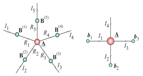
A full multilinear product of a tensor and a set of matrices takes into account all the modes, and can be compactly written as (see Fig 6 (a)):

𝐂¯¯𝐂\displaystyle\underline{{\bf C}} =\displaystyle= 𝐀¯×1𝐁(1)×2𝐁(2)×N𝐁(N)subscript𝑁subscript2subscript1¯𝐀superscript𝐁1superscript𝐁2superscript𝐁𝑁\displaystyle\underline{{\bf A}}\times_{1}{\bf B}^{(1)}\times_{2}{\bf B}^{(2)}\cdots\times_{N}{\bf B}^{(N)} (3)
=\displaystyle= 𝐀¯;𝐁(1),𝐁(2),,𝐁(N).¯𝐀superscript𝐁1superscript𝐁2superscript𝐁𝑁\displaystyle\llbracket\underline{{\bf A}};{\bf B}^{(1)},{\bf B}^{(2)},\ldots,{\bf B}^{(N)}\rrbracket.

(a)                                    (b)
Refer to caption

Figure  6: (a) Multilinear product of tensor 𝐀¯R1×R2××R5¯𝐀superscriptsubscript𝑅1subscript𝑅2subscript𝑅5\underline{{\bf A}}\in\mathbb{R}^{R_{1}\times R_{2}\times\cdots\times R_{5}} and 5 factor (component) matrices 𝐁(n)In×Rnsuperscript𝐁𝑛superscriptsubscript𝐼𝑛subscript𝑅𝑛{\bf B}^{(n)}\in\mathbb{R}^{I_{n}\times R_{n}} (n=1,2,,5𝑛125n=1,2,\ldots,5) yields 𝐂¯=𝐀¯×1𝐁(1)×2𝐁(2)×3𝐁(3)×4𝐁(4)×5𝐁(5)I1×I2××I5¯𝐂subscript5subscript4subscript3subscript2subscript1¯𝐀superscript𝐁1superscript𝐁2superscript𝐁3superscript𝐁4superscript𝐁5superscriptsubscript𝐼1subscript𝐼2subscript𝐼5\underline{{\bf C}}=\underline{{\bf A}}\times_{1}{\bf B}^{(1)}\times_{2}{\bf B}^{(2)}\times_{3}{\bf B}^{(3)}\times_{4}{\bf B}^{(4)}\times_{5}{\bf B}^{(5)}\in\mathbb{R}^{I_{1}\times I_{2}\times\cdots\times I_{5}} and (b) Multilinear product of tensor 𝐀¯I1×I2×I3×I4¯𝐀superscriptsubscript𝐼1subscript𝐼2subscript𝐼3subscript𝐼4\underline{{\bf A}}\in\mathbb{R}^{I_{1}\times I_{2}\times I_{3}\times I_{4}} and vectors 𝒃nInsubscript𝒃𝑛superscriptsubscript𝐼𝑛\mbox{\boldmath$b$}_{n}\in\mathbb{R}^{I_{n}} (n=1,2,3)𝑛123(n=1,2,3) yields a vector 𝒄=𝐀¯×¯1𝒃1ׯ2𝒃2ׯ3𝒃3I4𝒄¯𝐀subscript¯1subscript𝒃1subscript¯2subscript𝒃2subscript¯3subscript𝒃3superscriptsubscript𝐼4\mbox{\boldmath$c$}=\underline{{\bf A}}\bar{\times}_{1}\mbox{\boldmath$b$}_{1}\bar{\times}_{2}\mbox{\boldmath$b$}_{2}\bar{\times}_{3}\mbox{\boldmath$b$}_{3}\in\mathbb{R}^{I_{4}}.

In a similar way, we can define the mode-(nm)(^{m}_{n}) product of two tensors 𝐀¯I1×I2××IN¯𝐀superscriptsubscript𝐼1subscript𝐼2subscript𝐼𝑁\underline{{\bf A}}\in\mathbb{R}^{I_{1}\times I_{2}\times\ldots\times I_{N}} and 𝐁¯J1×J2××JM¯𝐁superscriptsubscript𝐽1subscript𝐽2subscript𝐽𝑀\underline{{\bf B}}\in\mathbb{R}^{J_{1}\times J_{2}\times\cdots\times J_{M}} with common modes In=Jmsubscript𝐼𝑛subscript𝐽𝑚I_{n}=J_{m} that produces a (N+M2)𝑁𝑀2(N+M-2)-order tensor 𝐂¯I1×In1×In+1×IN×J1×Jm1×Jm+1×JM¯𝐂superscriptsubscript𝐼1subscript𝐼𝑛1subscript𝐼𝑛1subscript𝐼𝑁subscript𝐽1subscript𝐽𝑚1subscript𝐽𝑚1subscript𝐽𝑀\underline{{\bf C}}\in\mathbb{R}^{I_{1}\times\cdots I_{n-1}\times I_{n+1}\cdots\times I_{N}\times J_{1}\times\cdots J_{m-1}\times J_{m+1}\cdots\times J_{M}}:

𝐂¯=𝐀¯×nm𝐁¯,¯𝐂superscriptsubscript𝑛𝑚¯𝐀¯𝐁\displaystyle\underline{{\bf C}}=\underline{{\bf A}}\;\times_{n}^{m}\;\underline{{\bf B}}, (4)

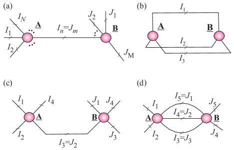
with entries ci1in1in+1iN,j1,jm1jm+1jM=i=1Inai1in1iin+1iNbj1jm1ijm+1jMsubscript𝑐subscript𝑖1subscript𝑖𝑛1subscript𝑖𝑛1subscript𝑖𝑁subscript𝑗1subscript𝑗𝑚1subscript𝑗𝑚1subscript𝑗𝑀superscriptsubscript𝑖1subscript𝐼𝑛subscript𝑎subscript𝑖1subscript𝑖𝑛1𝑖subscript𝑖𝑛1subscript𝑖𝑁subscript𝑏subscript𝑗1subscript𝑗𝑚1𝑖subscript𝑗𝑚1subscript𝑗𝑀c_{i_{1}\cdots i_{n-1}\,i_{n+1}\cdots i_{N},\,j_{1},\cdots j_{m-1}\,j_{m+1}\cdots j_{M}}=\sum_{i=1}^{I_{n}}a_{i_{1}\cdots i_{n-1}\;i\;i_{n+1}\cdots i_{N}}b_{j_{1}\cdots j_{m-1}\;i\;j_{m+1}\cdots j_{M}} (see Fig. 7) (a).

Refer to caption
Figure  7: Examples of contraction of two tensors: (a) Multilinear product of two tensors is denoted by 𝐂¯=𝐀¯×nm𝐁¯¯𝐂superscriptsubscript𝑛𝑚¯𝐀¯𝐁\underline{{\bf C}}=\underline{{\bf A}}\;\times_{n}^{m}\;\underline{{\bf B}}. (b) Inner product of two 3rd-order tensors yields c=𝐀¯,𝐁¯=𝐀¯×1,2,31,2,3𝐁¯=𝐀¯×𝐁¯=i1,i2,i3ai1,i2,i3bi1,i2,i3𝑐¯𝐀¯𝐁superscriptsubscript123123¯𝐀¯𝐁¯𝐀¯𝐁subscriptsubscript𝑖1subscript𝑖2subscript𝑖3subscript𝑎subscript𝑖1subscript𝑖2subscript𝑖3subscript𝑏subscript𝑖1subscript𝑖2subscript𝑖3c=\langle\underline{{\bf A}},\underline{{\bf B}}\rangle=\underline{{\bf A}}\;\times_{1,2,3}^{1,2,3}\;\underline{{\bf B}}=\underline{{\bf A}}\;\times\;\underline{{\bf B}}=\sum_{i_{1},i_{2},i_{3}}\;a_{i_{1},i_{2},i_{3}}\;b_{i_{1},i_{2},i_{3}}. (c) Tensor contraction of two 4th-order tensors yields the 6h-order tensor 𝐂¯=𝐀¯×32𝐁¯I1×I2×I4×J1×J3×J4¯𝐂superscriptsubscript32¯𝐀¯𝐁superscriptsubscript𝐼1subscript𝐼2subscript𝐼4subscript𝐽1subscript𝐽3subscript𝐽4\underline{{\bf C}}=\underline{{\bf A}}\;\times_{3}^{2}\;\underline{{\bf B}}\in\mathbb{R}^{I_{1}\times I_{2}\times I_{4}\times J_{1}\times J_{3}\times J_{4}}, with entries ci1,i2,i4,j1,j3,j4=i3ai1,i2,i3,i4bj1,i3,j3,j4subscript𝑐subscript𝑖1subscript𝑖2subscript𝑖4subscript𝑗1subscript𝑗3subscript𝑗4subscriptsubscript𝑖3subscript𝑎subscript𝑖1subscript𝑖2subscript𝑖3subscript𝑖4subscript𝑏subscript𝑗1subscript𝑖3subscript𝑗3subscript𝑗4c_{i_{1},i_{2},i_{4},j_{1},j_{3},j_{4}}=\sum_{i_{3}}\;a_{i_{1},i_{2},i_{3},i_{4}}\;b_{j_{1},i_{3},j_{3},j_{4}}. (d) Tensor contraction of two 5th-order tensors yields the 4th-order tensor 𝐂¯=𝐀¯×3,4,51,2,3𝐁¯I1×I2×J4×J5¯𝐂superscriptsubscript345123¯𝐀¯𝐁superscriptsubscript𝐼1subscript𝐼2subscript𝐽4subscript𝐽5\underline{{\bf C}}=\underline{{\bf A}}\;\times_{3,4,5}^{1,2,3}\;\underline{{\bf B}}\in\mathbb{R}^{I_{1}\times I_{2}\times J_{4}\times J_{5}}, with entries ci1,i2,j4,j5=i3,i4,i5ai1,i2,i3,i4,i5bi5,i4,i3,j4,j5subscript𝑐subscript𝑖1subscript𝑖2subscript𝑗4subscript𝑗5subscriptsubscript𝑖3subscript𝑖4subscript𝑖5subscript𝑎subscript𝑖1subscript𝑖2subscript𝑖3subscript𝑖4subscript𝑖5subscript𝑏subscript𝑖5subscript𝑖4subscript𝑖3subscript𝑗4subscript𝑗5c_{i_{1},i_{2},j_{4},j_{5}}=\sum_{i_{3},i_{4},i_{5}}\;a_{i_{1},i_{2},i_{3},i_{4},i_{5}}\;b_{i_{5},i_{4},i_{3},j_{4},j_{5}}.

When not confusing, the super-index m𝑚m can be neglected. For example, the mode-1 product of the tensors 𝐀¯I1×I2××IN¯𝐀superscriptsubscript𝐼1subscript𝐼2subscript𝐼𝑁\underline{{\bf A}}\in\mathbb{R}^{I_{1}\times I_{2}\times\cdots\times I_{N}} and 𝐁¯J1×J2××JM¯𝐁superscriptsubscript𝐽1subscript𝐽2subscript𝐽𝑀\underline{{\bf B}}\in\mathbb{R}^{J_{1}\times J_{2}\times\cdots\times J_{M}}, with a common first mode I1=J1subscript𝐼1subscript𝐽1I_{1}=J_{1} can be written as

𝐂¯=𝐀¯×11𝐁¯=𝐀¯×1𝐁¯I2××IN×J2××JM,¯𝐂superscriptsubscript11¯𝐀¯𝐁subscript1¯𝐀¯𝐁superscriptsubscript𝐼2subscript𝐼𝑁subscript𝐽2subscript𝐽𝑀\displaystyle\underline{{\bf C}}=\underline{{\bf A}}\;\times_{1}^{1}\;\underline{{\bf B}}=\underline{{\bf A}}\times_{1}\underline{{\bf B}}\in\mathbb{R}^{I_{2}\times\cdots\times I_{N}\times J_{2}\times\cdots\times J_{M}}, (5)

with entries c𝒊2:N,𝒋2:M=i=1I1ai,𝒊2:Nbi,𝒋2:Msubscript𝑐subscript𝒊:2𝑁subscript𝒋:2𝑀superscriptsubscript𝑖1subscript𝐼1subscript𝑎𝑖subscript𝒊:2𝑁subscript𝑏𝑖subscript𝒋:2𝑀c_{\mbox{\boldmath$i$}_{2:N},\mbox{\boldmath$j$}_{2:M}}=\sum_{i=1}^{I_{1}}a_{i,\mbox{\boldmath$i$}_{2:N}}b_{i,\mbox{\boldmath$j$}_{2:M}}, when using MATLAB notation, 𝒊p:q={ip,ip+1,,iq1,iq}subscript𝒊:𝑝𝑞subscript𝑖𝑝subscript𝑖𝑝1subscript𝑖𝑞1subscript𝑖𝑞\mbox{\boldmath$i$}_{p:q}=\{i_{p},i_{p+1},\ldots,i_{q-1},i_{q}\}. This operation can be considered as a tensor contraction of two modes. Tensors can be contracted in several modes or even in all modes (see Fig. 7).

Tensor contraction is a fundamental operation, which can be considered as a higher dimensional analogue of inner product, outer product and matrix multiplications, and comprises computationally dominant operations in most numerical algorithms. However, unlike the matrix by matrix multiplications for which many efficient distributed-memory parallel schemes have been developed, for a tensor contraction we have a rather limited number of available optimized algorithms [24, 25, 26]. In practice, we usually implement approximate tensors contractions with reduced ranks [27]. A significant help in developing effective distributed tensor contraction algorithms is that the tensors used in computational models often exhibit symmetry over all or multiple modes; exploitation of the symmetry is essential, both in order to save on storage as well as to avoid unnecessary arithmetic operations [25, 26].

(a)
Refer to caption
(b)
Refer to caption

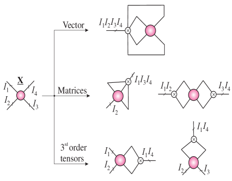
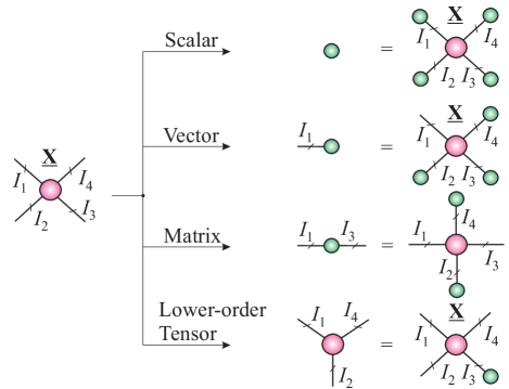
Figure  8: (a) Transforming or compressing a 4th-order tensor into scalar, vector, matrix and 3rd-order tensor by multilinear product of the tensor and vectors. (b) Reshaping of a tensor by its vectorization, unfolding and reducing the order by merging the modes.
Refer to caption
Refer to caption
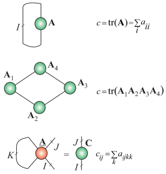
Figure  9: Tensor network notation and operations for traces of matrices and higher-order tensors.

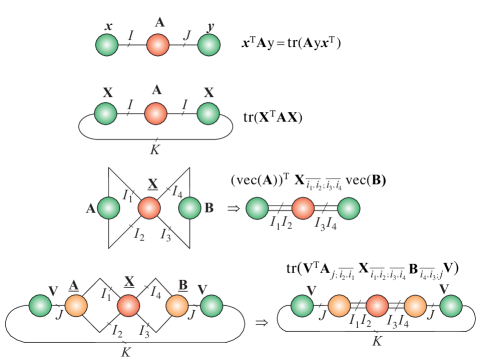
Tensors often need to be converted to traces, scalars, vectors, matrices or tensors with reshaped modes and reduced orders, as illustrated in Fig. 8 and Fig. 9.

III Low-Rank Tensor Approximations via Tensor Networks

III-A Basic Tensor Network Models

Tensor networks can be considered as a new “language” for big data tensor decompositions in simulation of large complex systems (e.g., in condensed matter physics and quantum physics) even with using standard computers [15, 28, 29, 2]. In other words, tensor networks, can be considered as a diagrammatic language for capturing the internal structure of high-order tensor decompositions.

In contrast to the CPD or Tucker decompositions, that have only one single core tensor, TNs decompose a high-order tensor into several lower-order core tensors. The branches (leads, lines, edges) connecting core tensors between each other correspond to contracted modes (and represent a TN rank), whereas lines that do not go from one tensor to another correspond to physical modes in the TN. A tensor network is a set of weakly connected core tensors, where some or all indices are contracted according to some rules.

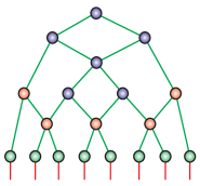
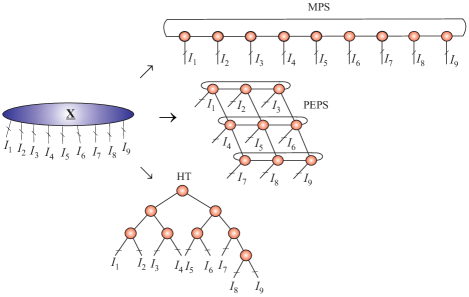
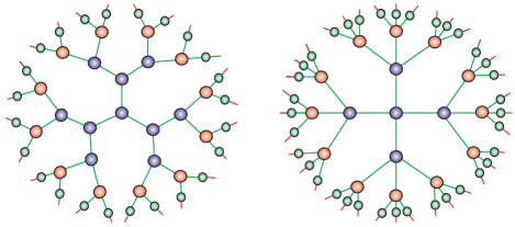
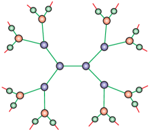
Some examples of basic tensor network diagrams are given in Figs. 10, 11, 12, and 13 [2, 14]. A tensor network may not contain any loops, i.e., any edges connecting a node with itself. If a tensor network is a binary tree, i.e., if it does not contain any cycles (loops), each of its edges splits the modes of the data tensor into two or more groups, which is related to the suitable matricization of the tensor [30, 31]. A tree tensor network, whose all nodes have degree 3 or 4, corresponds to a Hierarchical Tucker (HT) decomposition of the tensor illustrated in Fig. 13 (a). The HT decompositions in the numerical analysis community have been introduced by Hackbusch and Kühn [32] and Grasedyck [33] (see also [30, 34, 35, 36, 37] and references therein). The general construction of the HT decomposition requires a hierarchical splitting of the modes (with sizes I1,I2,,INsubscript𝐼1subscript𝐼2subscript𝐼𝑁I_{1},I_{2},\ldots,I_{N}). The construction of Hierarchical Tucker format relies on the notion of a dimension tree, chosen a priori, which specifies the topology of the HT decomposition. Intuitively, the dimension tree specifies which groups of modes are “separated” from other groups of modes, where sequential HT decomposition can be performed via (truncated) SVD applied to unfolded matrices [30].
Refer to caption
Figure  10: Illustration of decomposition of 9th-order tensor 𝐗¯I1×I2××I9¯𝐗superscriptsubscript𝐼1subscript𝐼2subscript𝐼9\underline{{\bf X}}\in\mathbb{R}^{I_{1}\times I_{2}\times\cdots\times I_{9}} into different forms of tensor networks (TNs): The Matrix Product State (MPS) with periodic boundary conditions (PBC), called also the Tensor Chain (TC), the Projected Entangled-Pair States (PEPS) with PBC and Hierarchical Tucker (HT) decomposition, which is equivalent to the Tree Tensor Network State (TTNS). In general, the objective is to decompose very high-order tensor into sparsely (weakly) connected low-order and low-rank tensors, typically 3rd-order and 4th-order tensors, called cores.
Refer to caption
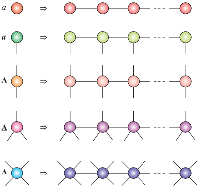
Figure  11: Different forms of tensor train decompositions depending on input data: For scalar functions a𝑎a, vectors 𝒂𝒂a, matrices 𝐀𝐀{\bf A}, and 3rd-order and 4th-order tensors 𝐀¯¯𝐀\underline{{\bf A}}.
Refer to caption
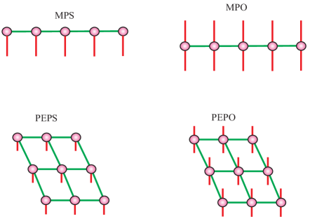
Figure  12: Basic tensor networks with open boundary conditions (OBC): The Matrix Product State (MPS) or (vector) Tensor Train (TT), the Matrix Product Operator (MPO) or Matrix TT, the Projected Entangled-Pair States (PEPS) or Tensor Product State (TPS) and the Projected Entangled-Pair Operators (PEPO).

(a) Hierarchical Tucker (HT) or Tree Tensor Network State (TTNS) with 3rd-order and 4th-order cores
Refer to caption
Refer to caption

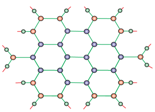
(b) Honey-Comb lattice for a 16th-order data tensor
Refer to caption

(c) MERA for 8th-order tensor

Refer to caption
Figure  13: Architectures of the fundamental TNs, which can be considered as distributed models of the Tucker-N𝑁N models. Green nodes denote factor matrices, while blue and red nodes denote cores.

The Tensor Train (TT) format proposed in the numerical analysis community by Oseledets and Tyrtyshnikow [38] (see also [39, 40, 13, 41, 42, 43]) can be interpreted as a special case of the HT, where all nodes of the underlying tensor network are aligned and where, moreover, the leaf matrices are assumed to be identities (and thus need not be stored). An advantage of the TT format is its simpler practical implementation, as no binary tree need be involved. The Tensor Trains [38, 40, 44], called also Matrix Product States (MPS) in quantum information theory [45, 46, 15, 47, 48], is the simplest TN model222In fact, the TT was rediscovered several times under different names: MPS, valence bond states and density matrix renormalization group (DMRG). The DMRG usually means not only tensor format but also power-full computational algorithms (see [49] and references therein)..

For some very high-order data tensors it has been observed that the ranks Rnsubscript𝑅𝑛R_{n} of 3rd-order tensors increase rapidly with the order of the tensor, for any choice of tensor network that is a tree (including TT and HT decompositions) [35].

For such cases, PEPS and the Multi-scale Entanglement Renormalization Ansatz (MERA) tensor networks can be used which contain cycles, but have hierarchical structures (see Fig. 13) (c). For the PEPS and MERA TNs the ranks can be kept considerably smaller, at the cost of employing 5th and 4th-order core tensors and consequently a higher computational complexity w.r.t. their ranks [50, 51].

Some interesting connections between tensor networks and graphical models used extensively in machine learning and statistics as shown in Table II [52, 53, 54, 41, 55]. Despite clear analogy, more research is needed to find more deep and precise relationships [55].

TABLE II: Similarities and links between tensor networks (TNs) and graphical models used in Machine Learning (ML) and Statistics. The categories are not exactly the same, but they closely correspond.

Tensor Networks Graphical Models in ML/Statistics TT/MPS Hidden Markov Models (HMM) HT/TTNS Gaussian Mixture Model (GMM) TNS/PEPS Markov Random Field (MRF) and Conditional Random Field (CRF) MERA Deep Belief Networks (DBN) DMRG and MALS Algs. Forward-Backward Algs., Block Nonlinear Gauss-Seidel Methods

III-B Changing the Structure of Tensor Networks

One advantage of a graphical representation of a tensor network is that it allows us to perform even most c complex mathematical operations in intuitive and easy to understand way. Another important advantage is the ability to modify or optimize a TN structure, that is, to change its topology, preserving physical modes unchanged. In fact, in some applications it is quite useful to modify the topology of a tensor network with or without approximation by providing simplified or more convenient graphical representation of the same higher-order data tensor [56, 57, 58]. For instance, tensor networks may consist of many cycles, those can t be reduced or completely eliminated in order to reduce computational complexity of contraction of core tensors and to provide stability of computation. Again, observe a strong link with loop elimination in control theory, in addition tensor networks having many cycles may not admit stable algorithm. By changing the topology to a tree structure (TT/HT models), we can often reduce complexity of computation and improve stability of algorithms.

(a)
Refer to caption
(b)
Refer to caption
(c)
Refer to caption

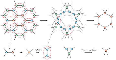
Figure  14: Illustration of basic transformation of tensors via: (a) Contraction, unfolding, matrix factorization (SVD) and reshaping of matrices back into tensors. (b) Transformation of Honey-Comb lattice into Tensor Chain (TC) via tensor contractions and the SVD. (c) Transformation of the TC, i.e., a TT/MPS with periodic boundary conditions (PBC) to the standard TT, i.e., the MPS with open boundary conditions (OBC).

Performing contraction of core tensors iteratively for tree–structured tensor networks has usually a much smaller complexity than tensor networks containing many cycles. One could transform a specific tensor network with cycles into a tree structure, perform stable computations333The TT decomposition is stable in the sense that the best approximation of a data tensor with bounded TT-ranks always exist and a quasi-optimal approximation can be computed by a sequence of truncated SVDs of suitably reshaping matrices of cores [39, 40]., with it and re-transform it back to the original structure if necessary. Furthermore, in the cases that we need to compare or analyze a set of blocks of tensor data, it is important that such tensors are represented by the same or very similar structures to analyze link or correlation between them or detect common cores or hidden components. Performing such analysis with differently structured tensor networks is in general difficult or even impossible.

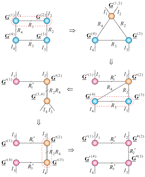
A Tensor network can be relatively easily transformed from one form to another one via tensor contractions, reshaping and basic matrix factorizations, typically using SVD [39, 40]. The basic approach to modify tensor structure is to perform: sequential core contractions, unfolding contracting tensors into matrices, performing matrix factorizations (typically, SVD) and finally reshaping matrices back to new core tensors. These principles are illustrated graphically in Figs 14 (a), (b), (c).

For example, in Fig 14 (a) in the first step we perform a contraction of two core tensors 𝐆¯(1)I1×I2×Rsuperscript¯𝐆1superscriptsubscript𝐼1subscript𝐼2𝑅\underline{{\bf G}}^{(1)}\in\mathbb{R}^{I_{1}\times I_{2}\times R} and 𝐆¯(2)R×I3×I4superscript¯𝐆2superscript𝑅subscript𝐼3subscript𝐼4\underline{{\bf G}}^{(2)}\in\mathbb{R}^{R\times I_{3}\times I_{4}}, as:

𝐆¯(1,2)=𝐆¯(1)×31𝐆¯(2)I1×I2×I3×I4,superscript¯𝐆12superscriptsubscript31superscript¯𝐆1superscript¯𝐆2superscriptsubscript𝐼1subscript𝐼2subscript𝐼3subscript𝐼4\displaystyle\underline{{\bf G}}^{(1,2)}=\underline{{\bf G}}^{(1)}\times_{3}^{1}\;\underline{{\bf G}}^{(2)}\in\mathbb{R}^{I_{1}\times I_{2}\times I_{3}\times I_{4}}, (6)

with entries gi1,i2,i3,i4(1,2)=r=1Rgi1,i2,r(1)gr,i3,i4(2)superscriptsubscript𝑔subscript𝑖1subscript𝑖2subscript𝑖3subscript𝑖412superscriptsubscript𝑟1𝑅superscriptsubscript𝑔subscript𝑖1subscript𝑖2𝑟1superscriptsubscript𝑔𝑟subscript𝑖3subscript𝑖42g_{i_{1},i_{2},i_{3},i_{4}}^{(1,2)}=\sum_{r=1}^{R}g_{i_{1},i_{2},r}^{(1)}\;g_{r,i_{3},i_{4}}^{(2)}. In the next step, we transform the tensor 𝐆¯(1,2)superscript¯𝐆12\underline{{\bf G}}^{(1,2)} into a matrix via unfolding and low-rank matrix factorization via the SVD

𝐆i1,i4¯;i2,i3¯(1,2)𝐔𝚺𝐕TI1I4×I2I3.subscriptsuperscript𝐆12¯subscript𝑖1subscript𝑖4¯subscript𝑖2subscript𝑖3𝐔𝚺superscript𝐕𝑇superscriptsubscript𝐼1subscript𝐼4subscript𝐼2subscript𝐼3\displaystyle{\bf G}^{(1,2)}_{\overline{i_{1},i_{4}};\overline{i_{2},i_{3}}}\cong{\bf U}\mbox{\boldmath$\Sigma$}{\bf V}^{T}\in\mathbb{R}^{I_{1}I_{4}\times I_{2}I_{3}}. (7)

In the last step, we reshape factor matrices 𝐔𝚺1/2I1I4×R𝐔superscript𝚺12superscriptsubscript𝐼1subscript𝐼4superscript𝑅{\bf U}\mbox{\boldmath$\Sigma$}^{1/2}\in\mathbb{R}^{I_{1}I_{4}\times R^{\prime}} and 𝐕𝚺1/2R×I2I3𝐕superscript𝚺12superscriptsuperscript𝑅subscript𝐼2subscript𝐼3{\bf V}\mbox{\boldmath$\Sigma$}^{1/2}\in\mathbb{R}^{R^{\prime}\times I_{2}I_{3}} back to new core tensors: 𝐆¯(1)I1×R×I4\underline{{\bf G}}^{{}^{\prime}(1)}\in\mathbb{R}^{I_{1}\times R^{\prime}\times I_{4}} and 𝐆¯(2)I2×I3×R\underline{{\bf G}}^{{}^{\prime}(2)}\in\mathbb{R}^{I_{2}\times I_{3}\times R^{\prime}}.

The above procedure has been applied in Fig. 14 (b) to transform Honey-Comb lattice into tensor chain (TC) along with tensor contraction of three cores [57].

In Fig. 14 (c) we have illustrated how to convert tensor chain (TC) into TT/MPS with OBC, by contracting sequentially two core tensors, unfolding them, applying SVD and reshaping matrices back into core tensors [56]. More precisely, in the first step, we perform a contraction of two tensors 𝐆¯(1)I1×R4×R1superscript¯𝐆1superscriptsubscript𝐼1subscript𝑅4subscript𝑅1\underline{{\bf G}}^{(1)}\in\mathbb{R}^{I_{1}\times R_{4}\times R_{1}} and 𝐆¯(2)R1×R2×I2superscript¯𝐆2superscriptsubscript𝑅1subscript𝑅2subscript𝐼2\underline{{\bf G}}^{(2)}\in\mathbb{R}^{R_{1}\times R_{2}\times I_{2}}, as:

𝐆¯(1,2)=𝐆¯(1)×31𝐆¯(2)I1×R4×R2×I2,superscript¯𝐆12superscriptsubscript31superscript¯𝐆1superscript¯𝐆2superscriptsubscript𝐼1subscript𝑅4subscript𝑅2subscript𝐼2\displaystyle\underline{{\bf G}}^{(1,2)}=\underline{{\bf G}}^{(1)}\times_{3}^{1}\;\underline{{\bf G}}^{(2)}\in\mathbb{R}^{I_{1}\times R_{4}\times R_{2}\times I_{2}}, (8)

with entries gi1,r4,r2,i2(1,2)=r1=1R1gi1,r4,r1(1)gr1,r2,i2(2)superscriptsubscript𝑔subscript𝑖1subscript𝑟4subscript𝑟2subscript𝑖212superscriptsubscriptsubscript𝑟11subscript𝑅1superscriptsubscript𝑔subscript𝑖1subscript𝑟4subscript𝑟11superscriptsubscript𝑔subscript𝑟1subscript𝑟2subscript𝑖22g_{i_{1},r_{4},r_{2},i_{2}}^{(1,2)}=\sum_{r_{1}=1}^{R_{1}}g_{i_{1},r_{4},r_{1}}^{(1)}\;g_{r_{1},r_{2},i_{2}}^{(2)}. In the next step, we can transform this tensor 𝐆¯(1,2)superscript¯𝐆12\underline{{\bf G}}^{(1,2)} into a matrix in order to perform the truncated SVD:

𝐆i1;r4,r2,i2¯(1,2)𝐔𝚺𝐕TI1×R4R2I2.subscriptsuperscript𝐆12subscript𝑖1¯subscript𝑟4subscript𝑟2subscript𝑖2𝐔𝚺superscript𝐕𝑇superscriptsubscript𝐼1subscript𝑅4subscript𝑅2subscript𝐼2\displaystyle{\bf G}^{(1,2)}_{i_{1}\,;\,\overline{r_{4},r_{2},i_{2}}}\cong{\bf U}\mbox{\boldmath$\Sigma$}{\bf V}^{T}\in\mathbb{R}^{I_{1}\times R_{4}R_{2}I_{2}}. (9)

In the next step, we reshape orthogonal matrices 𝐔𝚺1/2I1×R1𝐔superscript𝚺12superscriptsubscript𝐼1subscriptsuperscript𝑅1{\bf U}\mbox{\boldmath$\Sigma$}^{1/2}\in\mathbb{R}^{I_{1}\times R^{\prime}_{1}} and 𝐕𝚺1/2R1×R4R2I2𝐕superscript𝚺12superscriptsubscriptsuperscript𝑅1subscript𝑅4subscript𝑅2subscript𝐼2{\bf V}\mbox{\boldmath$\Sigma$}^{1/2}\in\mathbb{R}^{R^{\prime}_{1}\times R_{4}R_{2}I_{2}} back to core tensors: 𝐆¯(1)=𝐔𝚺1/21×I1×R1\underline{{\bf G}}^{{}^{\prime}(1)}={\bf U}\mbox{\boldmath$\Sigma$}^{1/2}\in\mathbb{R}^{1\times I_{1}\times R^{\prime}_{1}} and 𝐆¯(2)R1×R4×R2×I2\underline{{\bf G}}^{{}^{\prime}(2)}\in\mathbb{R}^{R^{\prime}_{1}\times R_{4}\times R_{2}\times I_{2}}. The procedure is repeated again and again for different pair of cores as illustrated in the Fig. 14 (c).

III-C Distributed (Concatenated) Representation of Tensors

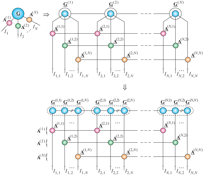
(a) Tensor Train (TT) model – MPS/MPO with the Open Boundary Conditions (OBC)
Refer to caption

(b) Tensor Chain (TC) model – MPS/MPO with the Periodic Boundary Conditions (PBC)
Refer to caption
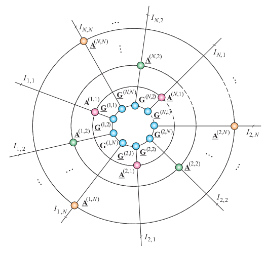
Figure  15: New distributed models of the Tucker-N𝑁N decomposition 𝐗¯=𝐆¯×1𝐀(1)×2𝐀(2)×N𝐀(N)I1×I2×IN¯𝐗subscript𝑁subscript2subscript1¯𝐆superscript𝐀1superscript𝐀2superscript𝐀𝑁superscriptsubscript𝐼1subscript𝐼2subscript𝐼𝑁\underline{{\bf X}}=\underline{{\bf G}}\times_{1}{\bf A}^{(1)}\times_{2}{\bf A}^{(2)}\cdots\times_{N}{\bf A}^{(N)}\in\mathbb{R}^{I_{1}\times I_{2}\times\cdots I_{N}}, with In=I1,nI2,nIN,n,subscript𝐼𝑛subscript𝐼1𝑛subscript𝐼2𝑛subscript𝐼𝑁𝑛I_{n}=I_{1,n}I_{2,n}\cdots I_{N,n},\; (n=1,2,,N)𝑛12𝑁(n=1,2,\ldots,N).

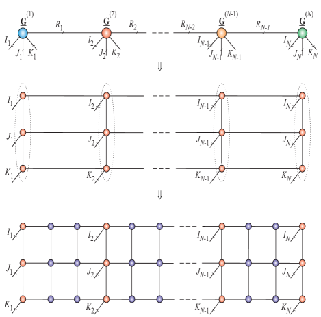
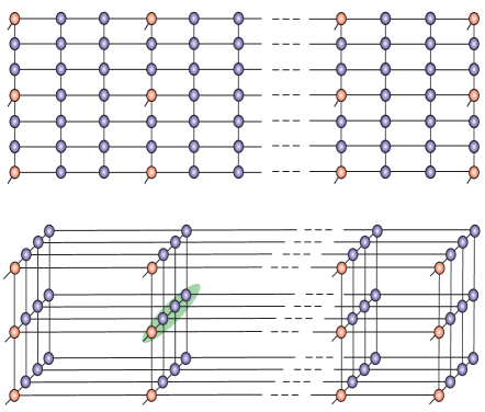
A simple approach to reduce the size or rank of core tensors is to apply distributed tensor networks (DTNs), which consists of two kind of cores (nodes): internal nodes which has no free edges and external nodes which have free edges representing natural (physical) indices of a data tensor as illustrated in Figs. 13 and 15. A simple idea is that each of the core tensor in an original TN is itself repeatedly replaced by another TN (see Fig. 16), resulting in another TN in which only some core tensors are associated with physical (natural) modes of the original data tensor [58].
Refer to caption
Refer to caption
Figure  16: Graphical representation of TT via Tensor Product State (TPS) or equivalently PEPS for a large-scale data tensor and its transformation to distributed 2D and 3D PEPS [58].

The main advantage of DTNs is that the size of each of the core tensors in the internal tensor network structure is usually much smaller than the initial core tensor so consequently the total number of parameters can be reduced [58]. However, it should be noted that the contraction of the resulting tensor network becomes more difficult when compared to the initial tree structure. This is due to the fact that the distributed tensor network contains loops.

Many algorithms applied to tensor networks scale with the size Rksubscript𝑅𝑘R_{k} or Iksubscript𝐼𝑘I_{k} of the core tensors of the network. In spite of the usually polynomial scaling of these algorithms, the computations quickly become intractable for increasing Rksubscript𝑅𝑘R_{k}, so that a network containing core tensors with small dimensions are favorable in general. See as examples the distributed Tucker models shown in Fig. 15 (a) and (b).

IV Tensorization – Blessing of Dimensionality

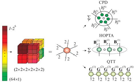
The procedure of creating a higher-order tensor from lower-order original data is referred to as tensorization. In other words, lower-order data tensors can be reshaped (reformatted) into high-order tensors. The purpose of a such tensorization or reshaping is to achieve a low-rank approximation with high level of compression. For example, big vectors, matrices even low-order tensors can be easily tensorized to very high-order tensors, then efficiently compressed by applying a suitable tensor network decomposition; this is the underlying principle for big data analysis [1, 2, 59, 16] (see also Figs.  17 - 20).
Refer to caption
Figure  17: The conceptual illustration of tensorization of a large-scale vector into a higher-order quantized tensor. In order to achieve super-compression we need to apply a suitable tensor decomposition: e.g., CPD decomposition into rank-1 tensors 𝐗¯r=1R𝒃r(1)𝒃r(2)𝒃r(6)¯𝐗superscriptsubscript𝑟1𝑅superscriptsubscript𝒃𝑟1superscriptsubscript𝒃𝑟2superscriptsubscript𝒃𝑟6\underline{{\bf X}}\cong\sum_{r=1}^{R}\mbox{\boldmath$b$}_{r}^{(1)}\circ\mbox{\boldmath$b$}_{r}^{(2)}\cdots\circ\mbox{\boldmath$b$}_{r}^{(6)}, Hierarchical Outer Product Tensor Approximation (HOPTA) using rank-q𝑞q terms: 𝐗¯r~=1R~𝐁r~(1)𝐁r~(2)𝐁r~(3)¯𝐗superscriptsubscript~𝑟1~𝑅superscriptsubscript𝐁~𝑟1superscriptsubscript𝐁~𝑟2superscriptsubscript𝐁~𝑟3\underline{{\bf X}}\cong\sum_{\tilde{r}=1}^{\tilde{R}}{\bf B}_{\tilde{r}}^{(1)}\circ{\bf B}_{\tilde{r}}^{(2)}\circ{\bf B}_{\tilde{r}}^{(3)} or quantized TT (QTT) using 3rd-order cores: 𝐗¯=𝐆¯(1)×31𝐆¯(2)×31×31𝐆¯(6)¯𝐗subscriptsuperscript13subscriptsuperscript13subscriptsuperscript13superscript¯𝐆1superscript¯𝐆2superscript¯𝐆6\underline{{\bf X}}=\underline{{\bf G}}^{(1)}\times^{1}_{3}\underline{{\bf G}}^{(2)}\times^{1}_{3}\cdots\times^{1}_{3}\underline{{\bf G}}^{(6)}.

IV-A Curse of Dimensionality

The term curse of dimensionality, in the context of tensors, refers to the fact that the number of elements of an N𝑁Nth-order (I×I××I)𝐼𝐼𝐼(I\times I\times\cdots\times I) tensor, INsuperscript𝐼𝑁I^{N}, grows exponentially with the tensor order N𝑁N. For example, for the Tucker decomposition the number of entries of an original data tensor but also a core tensor scales exponentially in the tensor order, for instance, the number of entries of an N𝑁Nth-order (R×R××R)𝑅𝑅𝑅(R\times R\times\cdots\times R) core tensor is RNsuperscript𝑅𝑁R^{N}.

If all computations are performed on a CP tensor format and not on the raw data tensor itself, then instead of the original INsuperscript𝐼𝑁I^{N} raw data entries, the number of parameters in a CP decomposition reduces to NRI𝑁𝑅𝐼NRI, which scales linearly in N𝑁N and I𝐼I. This effectively bypasses the curse of dimensionality, however the CP approximation may provide a poor fit to the data and may involve numerical problems, since existing CPD algorithms are not stable for high-order tensors. In this paper we exploit TT decompositions which are stable and robust with ability to control an approximation error i.e., to achieve any desired accuracy of TT approximation [40, 60]. The main idea of using low-rank tensor-structured approximations is to reduce the complexity of computation and relax or avoid the curse of dimensionality.

IV-B Quantized Tensor Networks

The curse of dimensionality can be overcome relatively easily through quantized tensor networks, which represent a tensor of possibly very high-order as a set of sparsely interconnected of low dimensions (typically, 3rd-order) cores [60, 59]. The concept of quantized tensor networks was first proposed by Oseledets [59] and Khoromskij [16].

(a)
Refer to caption

(b)

Refer to caption
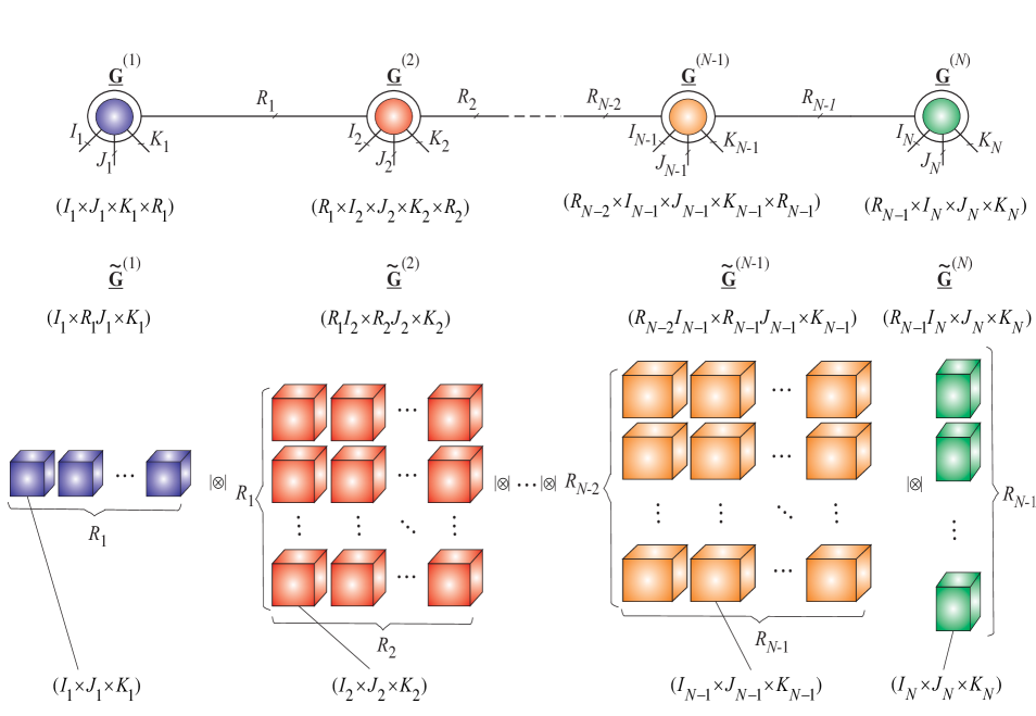
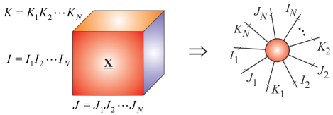
Figure  18: (a) Example 1 of tensorization and decomposition of a large-scale 3rd-order tensor 𝐗¯I×J×K¯𝐗superscript𝐼𝐽𝐾\underline{{\bf X}}\in\mathbb{R}^{I\times J\times K} into 3N3𝑁3Nth-order tensor, assuming that I=I1I2IN𝐼subscript𝐼1subscript𝐼2subscript𝐼𝑁I=I_{1}I_{2}\cdots I_{N}, J=J1J2JN𝐽subscript𝐽1subscript𝐽2subscript𝐽𝑁J=J_{1}J_{2}\cdots J_{N} and K=K1K2KN𝐾subscript𝐾1subscript𝐾2subscript𝐾𝑁K=K_{1}K_{2}\cdots K_{N}. (b) Decomposition of the tensor via generalized Tensor Train referred to as the Tensor Product State (TPS). The data tensor can be expressed by the strong Kronecker product of block tensors as 𝐗¯𝐆¯~(1)||𝐆¯~(2)||𝐆¯~(N)I1IN×J1JN×K1KN\underline{{\bf X}}\cong\underline{\widetilde{\bf G}}^{(1)}\;|\otimes|\;\underline{\widetilde{\bf G}}^{(2)}\;|\otimes|\cdots\otimes\;\underline{\widetilde{\bf G}}^{(N)}\in\mathbb{R}^{I_{1}\cdots I_{N}\times J_{1}\cdots J_{N}\times K_{1}\cdots K_{N}}, where each block of the core 𝐆¯~(n)Rn1In×RnJn×Knsuperscript¯~𝐆𝑛superscriptsubscript𝑅𝑛1subscript𝐼𝑛subscript𝑅𝑛subscript𝐽𝑛subscript𝐾𝑛\underline{\widetilde{\bf G}}^{(n)}\in\mathbb{R}^{R_{n-1}I_{n}\times R_{n}J_{n}\times K_{n}} is a 3rd-order tensor of size (In×Jn×Kn)subscript𝐼𝑛subscript𝐽𝑛subscript𝐾𝑛(I_{n}\times J_{n}\times K_{n}), with R0=RN=1subscript𝑅0subscript𝑅𝑁1R_{0}=R_{N}=1. The strong Kronecker product of two block cores 𝐆¯~(n)Rn1In×RnJn×Knsuperscript¯~𝐆𝑛superscriptsubscript𝑅𝑛1subscript𝐼𝑛subscript𝑅𝑛subscript𝐽𝑛subscript𝐾𝑛\underline{\widetilde{\bf G}}^{(n)}\in\mathbb{R}^{R_{n-1}I_{n}\times R_{n}J_{n}\times K_{n}} and 𝐆¯~(n+1)RnIn+1×Rn+1Jn+1×Kn+1superscript¯~𝐆𝑛1superscriptsubscript𝑅𝑛subscript𝐼𝑛1subscript𝑅𝑛1subscript𝐽𝑛1subscript𝐾𝑛1\underline{\widetilde{\bf G}}^{(n+1)}\in\mathbb{R}^{R_{n}I_{n+1}\times R_{n+1}J_{n+1}\times K_{n+1}} is defined as the block tensor 𝐂¯=𝐆¯~(n)||𝐆¯~(n+1)Rn1InIn+1×Rn+1JnJn+1×KnKn+1\underline{{\bf C}}=\underline{\widetilde{\bf G}}^{(n)}|\otimes|\underline{\widetilde{\bf G}}^{(n+1)}\in\mathbb{R}^{R_{n-1}I_{n}I_{n+1}\times R_{n+1}J_{n}J_{n+1}\times K_{n}K_{n+1}}, with 3rd-order tensor blocks 𝐂¯rn1,rn+1=rn=1Rn𝐆¯rn1,rn(n)𝐆¯rn,rn+1(n+1)InIn+1×JnJn+1×KnKn+1subscript¯𝐂subscript𝑟𝑛1subscript𝑟𝑛1superscriptsubscriptsubscript𝑟𝑛1subscript𝑅𝑛tensor-productsubscriptsuperscript¯𝐆𝑛subscript𝑟𝑛1subscript𝑟𝑛subscriptsuperscript¯𝐆𝑛1subscript𝑟𝑛subscript𝑟𝑛1superscriptsubscript𝐼𝑛subscript𝐼𝑛1subscript𝐽𝑛subscript𝐽𝑛1subscript𝐾𝑛subscript𝐾𝑛1\underline{{\bf C}}_{r_{n-1},r_{n+1}}=\sum_{r_{n}=1}^{R_{n}}\underline{{\bf G}}^{(n)}_{r_{n-1},r_{n}}\otimes\underline{{\bf G}}^{(n+1)}_{r_{n},r_{n+1}}\in\mathbb{R}^{I_{n}I_{n+1}\times J_{n}J_{n+1}\times K_{n}K_{n+1}}, where 𝐆¯rn1,rn(n)In×Jn×Knsubscriptsuperscript¯𝐆𝑛subscript𝑟𝑛1subscript𝑟𝑛superscriptsubscript𝐼𝑛subscript𝐽𝑛subscript𝐾𝑛\underline{{\bf G}}^{(n)}_{r_{n-1},r_{n}}\in\mathbb{R}^{I_{n}\times J_{n}\times K_{n}} and 𝐆¯rn,rn+1(n+1)In+1×Jn+1×Kn+1subscriptsuperscript¯𝐆𝑛1subscript𝑟𝑛subscript𝑟𝑛1superscriptsubscript𝐼𝑛1subscript𝐽𝑛1subscript𝐾𝑛1\underline{{\bf G}}^{(n+1)}_{r_{n},r_{n+1}}\in\mathbb{R}^{I_{n+1}\times J_{n+1}\times K_{n+1}} are block tensors of 𝐆¯~(n)superscript¯~𝐆𝑛\underline{\widetilde{\bf G}}^{(n)} and 𝐆¯~(n+1)superscript¯~𝐆𝑛1\underline{\widetilde{\bf G}}^{(n+1)}, respectively. In the special cases: J=K=1𝐽𝐾1J=K=1 and K=1𝐾1K=1 the model simplifies to standard tensor train models shown in Fig. 20 (a) and (b).

For example, the quantization and tensorization of a huge vector 𝐱I𝐱superscript𝐼{\bf x}\in\mathbb{R}^{I}, I=2K𝐼superscript2𝐾I=2^{K} can be achieved through reshaping to give an (2×2××2)222(2\times 2\times\cdots\times 2) tensor 𝐗¯¯𝐗\underline{{\bf X}} of order K𝐾K, as illustrated in Fig. 17. Such a quantized tensor 𝐗¯¯𝐗\underline{{\bf X}} often admits low-rank matrix/tensor approximations, so that a good compression of a huge vector 𝐱𝐱{\bf x} can be achieved by enforcing a maximum possible low-rank structure on the tensor 𝐗𝐗{\bf X}, thus admitting highly compressed representation via a tensor network.

Even more generally, an N𝑁Nth-order tensor 𝐗¯I1××IN¯𝐗superscriptsubscript𝐼1subscript𝐼𝑁\underline{{\bf X}}\in\mathbb{R}^{I_{1}\times\cdots\times I_{N}}, with In=qKnsubscript𝐼𝑛superscript𝑞subscript𝐾𝑛I_{n}=q^{K_{n}}, can be quantized in all modes simultaneously to yield a (q×q×q)𝑞𝑞𝑞(q\times q\times\cdots q) quantized tensor 𝐘¯¯𝐘\underline{{\bf Y}} of higher-order, with small q𝑞q.

In practice, a fine (q=2,3,4𝑞234q=2,3,4 ) quantization is desirable to create as many virtual modes as possible, thus allowing us to implement an efficient low-rank tensor approximations. For example, the binary encoding (q=2𝑞2q=2) reshapes an N𝑁Nth-order tensor with (2K1×2K2××2KN)superscript2subscript𝐾1superscript2subscript𝐾2superscript2subscript𝐾𝑁(2^{K_{1}}\times 2^{K_{2}}\times\cdots\times 2^{K_{N}}) elements into a tensor of order (K1+K2++KN)subscript𝐾1subscript𝐾2subscript𝐾𝑁(K_{1}+K_{2}+\cdots+K_{N}), with the same number of elements. In other words, the idea of the quantized tensor is quantization of the each n𝑛n-th “physical” mode (dimension) by replacing it with Knsubscript𝐾𝑛K_{n} “virtual” modes, provided that the corresponding mode size Insubscript𝐼𝑛I_{n} are factorized as In=In,1In,2In,Knsubscript𝐼𝑛subscript𝐼𝑛1subscript𝐼𝑛2subscript𝐼𝑛subscript𝐾𝑛I_{n}=I_{n,1}I_{n,2}\cdots I_{n,K_{n}}. This corresponds to reshaping the n𝑛n-th mode of size Insubscript𝐼𝑛I_{n} into Knsubscript𝐾𝑛K_{n} modes of sizes In,1,In,2,,In,Knsubscript𝐼𝑛1subscript𝐼𝑛2subscript𝐼𝑛subscript𝐾𝑛I_{n,1},I_{n,2},\ldots,I_{n,K_{n}}.

In example shown in Fig. 18, the Tensor Train of huge 3rd-order tensor is expressed by the strong Kronecker products of block tensors with relatively small 3rd-order tensor blocks. Since large-scale tensors cannot be loaded explicitly in main memory, they usually reside in distributed storage by splitting tensors to smaller blocks. Our approach is to apply tensor networks and represent big data by high-order tensors not explicitly but in compressed TT formats.

The TT decomposition applied to quantized tensors is referred to as the QTT; it was first introduced as a compression scheme for large-scale structured matrices, which admit low-rank TT approximation [59], and also developed for more general settings [16, 61, 62]. The attractive property of QTT is that not only its rank is typically small (below 10) but it is almost independent or at least uniformly bounded by data size, providing a logarithmic (sub-linear) reduction of storage requirements: 𝒪(IN)𝒪(Nlogq(I))𝒪superscript𝐼𝑁𝒪𝑁subscript𝑞𝐼{\cal{O}}(I^{N})\rightarrow{\cal{O}}(N\log_{q}(I)) – so-called super-compression [16].

Note also that, unlike in Tucker or CPD, the TT decomposition relies on a certain ordering of the modes so that reordering modes may affect the numerical values of TT ranks significantly.

Quantization is quite important for reducing the computational complexity further, since it allows the TT decomposition to resolve and represent more structure in the data by splitting the “virtual” dimensions introduced by the quantization, as well as the “physical” ones. In practice it appears the most efficient to use as fine a quantization as possible (typically, with q=2𝑞2q=2) and to generate as many virtual modes as possible.

A TT decomposition of the quantized vector is referred to as QTT decomposition of the original vector; the ranks of this TT decomposition are called ranks of the QTT decomposition of the original vector.

V Mathematical and Graphical Representation of Tensor Trains

In order to perform efficiently various mathematical operations in the TT formats we need to represent TT decompositions in compact and easily understandable mathematical and graphical representations [2, 13].

V-A Vector TT/MPS Decomposition

(a)
Refer to caption

(b)

Refer to caption
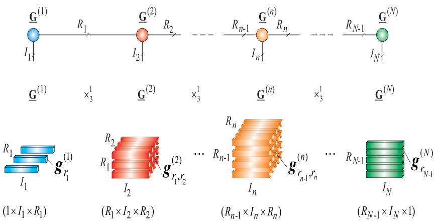
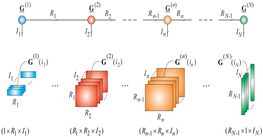
Figure  19: Alternative representations of the tensor train decomposition (TT/MPS) for an N𝑁Nth-order tensor 𝐗¯I1×I2×I3××IN¯𝐗superscriptsubscript𝐼1subscript𝐼2subscript𝐼3subscript𝐼𝑁\underline{{\bf X}}\in\mathbb{R}^{I_{1}\times I_{2}\times I_{3}\times\cdots\times I_{N}}; (a) Representation of the TT/MPS in a scalar form via slice matrices as: xi1,i2,,iN𝐆(1)(i1)𝐆(2)(i2)𝐆(N)(iN)=r1=1R1r2=1R2rN1=1RN1g1,i1,r1(1)gr1,i2,r2(2)gr2,i3,r3(3)grN1,iN,1(N)subscript𝑥subscript𝑖1subscript𝑖2subscript𝑖𝑁superscript𝐆1subscript𝑖1superscript𝐆2subscript𝑖2superscript𝐆𝑁subscript𝑖𝑁superscriptsubscriptsubscript𝑟11subscript𝑅1superscriptsubscriptsubscript𝑟21subscript𝑅2superscriptsubscriptsubscript𝑟𝑁11subscript𝑅𝑁1subscriptsuperscript𝑔11subscript𝑖1subscript𝑟1subscriptsuperscript𝑔2subscript𝑟1subscript𝑖2subscript𝑟2subscriptsuperscript𝑔3subscript𝑟2subscript𝑖3subscript𝑟3subscriptsuperscript𝑔𝑁subscript𝑟𝑁1subscript𝑖𝑁1x_{i_{1},i_{2},\ldots,i_{N}}\cong{\bf G}^{(1)}(i_{1})\;{\bf G}^{(2)}(i_{2})\;\cdots\;{\bf G}^{(N)}(i_{N})=\sum_{r_{1}=1}^{R_{1}}\sum_{r_{2}=1}^{R_{2}}\cdots\sum_{r_{N-1}=1}^{R_{N-1}}\;g^{(1)}_{1,i_{1},r_{1}}\;g^{(2)}_{r_{1},i_{2},r_{2}}\;g^{(3)}_{r_{2},i_{3},r_{3}}\;\cdots g^{(N)}_{r_{N-1},i_{N},1}; (b) expressed by the outer product of vectors (sum of rank-1 tensors) as: 𝐗¯r1=1R1r2=1R2rN1=1RN1(𝐠 1,r1(1)𝐠r1,r2(2)𝐠rN2,rN1(N1)𝐠rN1,1(N))¯𝐗superscriptsubscriptsubscript𝑟11subscript𝑅1superscriptsubscriptsubscript𝑟21subscript𝑅2superscriptsubscriptsubscript𝑟𝑁11subscript𝑅𝑁1subscriptsuperscript𝐠11subscript𝑟1subscriptsuperscript𝐠2subscript𝑟1subscript𝑟2subscriptsuperscript𝐠𝑁1subscript𝑟𝑁2subscript𝑟𝑁1subscriptsuperscript𝐠𝑁subscript𝑟𝑁11\underline{{\bf X}}\cong\sum_{r_{1}=1}^{R_{1}}\sum_{r_{2}=1}^{R_{2}}\cdots\sum_{r_{N-1}=1}^{R_{N-1}}({\bf g}^{(1)}_{\,1,r_{1}}\;\circ\;{\bf g}^{(2)}_{\,r_{1},r_{2}}\;\circ\cdots\circ{\bf g}^{(N-1)}_{\,r_{N-2},r_{N-1}}\;\circ\;{\bf g}^{(N)}_{\,r_{N-1},1}). All vectors 𝐠rn1rn(n)Insubscriptsuperscript𝐠𝑛subscript𝑟𝑛1subscript𝑟𝑛superscriptsubscript𝐼𝑛{\bf g}^{(n)}_{r_{n-1}r_{n}}\in\mathbb{R}^{I_{n}} are considered to be the column vectors.

The (vector) tensor train (TT/MPS) for N𝑁Nth-order data tensor 𝐗¯I1×I2××IN¯𝐗superscriptsubscript𝐼1subscript𝐼2subscript𝐼𝑁\underline{{\bf X}}\in\mathbb{R}^{I_{1}\times I_{2}\times\cdots\times I_{N}} can be described in the standard (tedious and rather complicated) scalar form as [63, 40]:

xi1,i2,,iNsubscript𝑥subscript𝑖1subscript𝑖2subscript𝑖𝑁\displaystyle x_{i_{1},i_{2},\ldots,i_{N}} \displaystyle\cong r1,r2,,rN1=1R1,R2,,RN1gi1,r1(1)gr1,i2,r2(2)grN1,iN(n)superscriptsubscriptsubscript𝑟1subscript𝑟2subscript𝑟𝑁11subscript𝑅1subscript𝑅2subscript𝑅𝑁1subscriptsuperscript𝑔1subscript𝑖1subscript𝑟1subscriptsuperscript𝑔2subscript𝑟1subscript𝑖2subscript𝑟2subscriptsuperscript𝑔𝑛subscript𝑟𝑁1subscript𝑖𝑁\displaystyle\sum_{r_{1},r_{2},\ldots,r_{N-1}=1}^{R_{1},R_{2},\ldots,R_{N-1}}g^{(1)}_{i_{1},r_{1}}\;g^{(2)}_{r_{1},i_{2},r_{2}}\cdots g^{(n)}_{r_{N-1},i_{N}}

or equivalently by using slice representations (see Fig. 19 (a)):

xi1,i2,,iN𝐆(1)(i1)𝐆(2)(i2)𝐆(N)(iN),subscript𝑥subscript𝑖1subscript𝑖2subscript𝑖𝑁superscript𝐆1subscript𝑖1superscript𝐆2subscript𝑖2superscript𝐆𝑁subscript𝑖𝑁\displaystyle x_{i_{1},i_{2},\ldots,i_{N}}\cong{\bf G}^{(1)}(i_{1})\;{\bf G}^{(2)}(i_{2})\cdots{\bf G}^{(N)}(i_{N}), (11)

where slice matrices are defined as

𝐆(n)(in)=𝐆(n)(:,in,:)Rn1×Rn,superscript𝐆𝑛subscript𝑖𝑛superscript𝐆𝑛:subscript𝑖𝑛:superscriptsubscript𝑅𝑛1subscript𝑅𝑛{\bf G}^{(n)}(i_{n})={\bf G}^{(n)}(:,i_{n},:)\in\mathbb{R}^{R_{n-1}\times R_{n}},

i.e., 𝐆(n)(in)superscript𝐆𝑛subscript𝑖𝑛{\bf G}^{(n)}(i_{n}) is an insubscript𝑖𝑛i_{n}th lateral slice of the core 𝐆¯(n)Rn1×In×Rnsuperscript¯𝐆𝑛superscriptsubscript𝑅𝑛1subscript𝐼𝑛subscript𝑅𝑛\underline{{\bf G}}^{(n)}\in\mathbb{R}^{R_{n-1}\times I_{n}\times R_{n}} for n=1,2,,N𝑛12𝑁n=1,2,\ldots,N, with R0=RN=1subscript𝑅0subscript𝑅𝑁1R_{0}=R_{N}=1.

However we can use several more convenient compact mathematical forms as follows (see Figs. 19 and 20(a) and Table III):

  1. 1.

    In a tensor form using multilinear products of cores:

    𝐗¯¯𝐗\displaystyle\underline{{\bf X}} \displaystyle\cong 𝐆¯(1)×31𝐆¯(2)×31×31𝐆¯(N1)×31𝐆¯(N)superscriptsubscript31superscriptsubscript31superscriptsubscript31superscriptsubscript31superscript¯𝐆1superscript¯𝐆2superscript¯𝐆𝑁1superscript¯𝐆𝑁\displaystyle\underline{{\bf G}}^{(1)}\times_{3}^{1}\underline{{\bf G}}^{(2)}\times_{3}^{1}\cdots\times_{3}^{1}\underline{{\bf G}}^{(N-1)}\times_{3}^{1}\underline{{\bf G}}^{(N)} (12)
    =\displaystyle= 𝐆¯(1),𝐆¯(2),,𝐆¯(N1),𝐆¯(N),superscript¯𝐆1superscript¯𝐆2superscript¯𝐆𝑁1superscript¯𝐆𝑁\displaystyle\llbracket\underline{{\bf G}}^{(1)},\underline{{\bf G}}^{(2)},\ldots,\underline{{\bf G}}^{(N-1)},\underline{{\bf G}}^{(N)}\rrbracket,

    where 3rd-order cores444Note that the cores 𝐆¯(1)superscript¯𝐆1\underline{{\bf G}}^{(1)} and 𝐆¯(N)superscript¯𝐆𝑁\underline{{\bf G}}^{(N)} are now two-dimensional arrays (matrices), but to apply uniform representation, we assume that 2nd-order cores are represented also as 3rd-order cores of mode sizes 1×I1×R11subscript𝐼1subscript𝑅11\times I_{1}\times R_{1} and RN1×IN×1subscript𝑅𝑁1subscript𝐼𝑁1R_{N-1}\times I_{N}\times 1, respectively. are defined as 𝐆¯(n)Rn1×In×Rnsuperscript¯𝐆𝑛superscriptsubscript𝑅𝑛1subscript𝐼𝑛subscript𝑅𝑛\underline{{\bf G}}^{(n)}\in\mathbb{R}^{R_{n-1}\times I_{n}\times R_{n}} for n=1,2,,,Nn=1,2,,\ldots,N with R0=RN=1subscript𝑅0subscript𝑅𝑁1R_{0}=R_{N}=1 (see Fig. 20(a)).

  2. 2.

    In tensor/vector form expressed as summation of rank-1 tensors, by using outer products of fibers (see Fig. 19 (b)):

    𝐗¯¯𝐗\displaystyle\underline{{\bf X}} \displaystyle\cong r1,r2,,rN1=1R1,R2,,RN1𝐠1,r1(1)𝐠r1,r2(2)𝐠rN1,1(N),superscriptsubscriptsubscript𝑟1subscript𝑟2subscript𝑟𝑁11subscript𝑅1subscript𝑅2subscript𝑅𝑁1subscriptsuperscript𝐠11subscript𝑟1subscriptsuperscript𝐠2subscript𝑟1subscript𝑟2subscriptsuperscript𝐠𝑁subscript𝑟𝑁11\displaystyle\sum_{r_{1},r_{2},\ldots,r_{N-1}=1}^{R_{1},R_{2},\ldots,R_{N-1}}{\bf g}^{(1)}_{1,r_{1}}\;\circ\;{\bf g}^{(2)}_{r_{1},r_{2}}\;\circ\;\cdots\circ\;{\bf g}^{(N)}_{r_{N-1},1},

    where 𝐠rn1,rn(n)=𝐆¯(n)(rn1,:,rn)Insubscriptsuperscript𝐠𝑛subscript𝑟𝑛1subscript𝑟𝑛superscript¯𝐆𝑛subscript𝑟𝑛1:subscript𝑟𝑛superscriptsubscript𝐼𝑛{\bf g}^{(n)}_{r_{n-1},r_{n}}=\underline{{\bf G}}^{(n)}(r_{n-1},\,:,\,r_{n})\in\mathbb{R}^{I_{n}} are mode-2 fibers, i.e., column vectors of matrices 𝐆(2)(n)=[𝐠1,1(n),𝐠2,1(n),,𝐠Rn1,1(n),𝐠1,2(n),,𝐠Rn1,Rn(n)]In×Rn1Rnsubscriptsuperscript𝐆𝑛2subscriptsuperscript𝐠𝑛11subscriptsuperscript𝐠𝑛21subscriptsuperscript𝐠𝑛subscript𝑅𝑛11subscriptsuperscript𝐠𝑛12subscriptsuperscript𝐠𝑛subscript𝑅𝑛1subscript𝑅𝑛superscriptsubscript𝐼𝑛subscript𝑅𝑛1subscript𝑅𝑛{\bf G}^{(n)}_{(2)}=[{\bf g}^{(n)}_{1,1},\;{\bf g}^{(n)}_{2,1},\ldots,{\bf g}^{(n)}_{R_{n-1},1},{\bf g}^{(n)}_{1,2},\ldots,{\bf g}^{(n)}_{R_{n-1},R_{n}}]\in\mathbb{R}^{I_{n}\times R_{n-1}R_{n}} (n=1,2,,N𝑛12𝑁n=1,2,\ldots,N), with R0=RN=1subscript𝑅0subscript𝑅𝑁1R_{0}=R_{N}=1 or equivalently in the vector form using the Kronecker products

    𝐱r1,r2,,rN1=1R1,R2,,RN1𝐠1,r1(1)𝐠r1,r2(2)𝐠rN1,1(N),𝐱superscriptsubscriptsubscript𝑟1subscript𝑟2subscript𝑟𝑁11subscript𝑅1subscript𝑅2subscript𝑅𝑁1tensor-productsubscriptsuperscript𝐠11subscript𝑟1subscriptsuperscript𝐠2subscript𝑟1subscript𝑟2subscriptsuperscript𝐠𝑁subscript𝑟𝑁11{\bf x}\cong\sum_{r_{1},r_{2},\ldots,r_{N-1}=1}^{R_{1},R_{2},\ldots,R_{N-1}}{\bf g}^{(1)}_{1,r_{1}}\;\otimes\;{\bf g}^{(2)}_{r_{1},r_{2}}\;\otimes\;\cdots\otimes\;{\bf g}^{(N)}_{r_{N-1},1},\\ (14)

    where the vector is defined as 𝐱=𝐱i1,i2,,iN¯=vec(𝐗)I1I2IN𝐱subscript𝐱¯subscript𝑖1subscript𝑖2subscript𝑖𝑁vec𝐗superscriptsubscript𝐼1subscript𝐼2subscript𝐼𝑁{\bf x}={\bf x}_{\overline{i_{1},i_{2},\ldots,i_{N}}}=\mbox{vec}({\bf X})\in\mathbb{R}^{I_{1}I_{2}\cdots I_{N}}.

  3. 3.

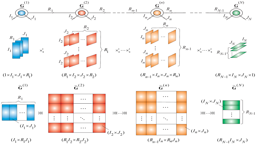
    In the vector form expressed by the strong Kronecker products of block matrices [64, 2] (see Fig. 20(a)):

    𝐱i1,i2,,iN¯𝐆~(1)||𝐆~(2)||||𝐆~(N),{\bf x}_{{\overline{i_{1},i_{2},\ldots,i_{N}}}}\cong\widetilde{\bf G}^{(1)}\;|\otimes|\;\widetilde{\bf G}^{(2)}\;|\otimes|\cdots|\otimes|\widetilde{\bf G}^{(N)},\\ (15)

    where the cores 𝐆¯(n)Rn1×In×Rnsuperscript¯𝐆𝑛superscriptsubscript𝑅𝑛1subscript𝐼𝑛subscript𝑅𝑛\underline{{\bf G}}^{(n)}\in\mathbb{R}^{R_{n-1}\times I_{n}\times R_{n}} are represented by block matrices 𝐆~(n)=(𝐆(3)(n))TRn1In×Rnsuperscript~𝐆𝑛superscriptsubscriptsuperscript𝐆𝑛3𝑇superscriptsubscript𝑅𝑛1subscript𝐼𝑛subscript𝑅𝑛\widetilde{\bf G}^{(n)}=({\bf G}^{(n)}_{(3)})^{T}\in\mathbb{R}^{R_{n-1}I_{n}\times R_{n}} for n=1,2,,N𝑛12𝑁n=1,2,\ldots,N, with blocks 𝐠rn1,rn(n)In×1subscriptsuperscript𝐠𝑛subscript𝑟𝑛1subscript𝑟𝑛superscriptsubscript𝐼𝑛1{\bf g}^{(n)}_{r_{n-1},r_{n}}\in\mathbb{R}^{I_{n}\times 1}, R0=RN=1subscript𝑅0subscript𝑅𝑁1R_{0}=R_{N}=1, and the symbol |||\otimes| denotes the strong Kronecker product.

TABLE III: Equivalent forms of the Tensor Trains (TT): MPS and MPO (with open boundary conditions) representation of an N𝑁Nth-order tensor 𝐗¯I1×I1××IN¯𝐗superscriptsubscript𝐼1subscript𝐼1subscript𝐼𝑁\underline{{\bf X}}\in\mathbb{R}^{I_{1}\times I_{1}\times\cdots\times I_{N}} and a 2N2𝑁2Nth-order tensor 𝐘¯I1×J1×I2×J2×IN×JN¯𝐘superscriptsubscript𝐼1subscript𝐽1subscript𝐼2subscript𝐽2subscript𝐼𝑁subscript𝐽𝑁\underline{{\bf Y}}\in\mathbb{R}^{I_{1}\times J_{1}\times I_{2}\times J_{2}\cdots\times I_{N}\times J_{N}}, respectively. It is assumed that the TT rank is {R1,R2,,RN1}subscript𝑅1subscript𝑅2subscript𝑅𝑁1\{R_{1},R_{2},\ldots,R_{N-1}\}, with R0=RN=1subscript𝑅0subscript𝑅𝑁1R_{0}=R_{N}=1.

                         TT/MPS                          TT/MPO Tensor Representations: Multilinear Products (tensor contractions) 𝐗¯=𝐆¯(1)×31𝐆¯(2)×31×31𝐆¯(N1)×31𝐆¯(N)¯𝐗superscriptsubscript31superscriptsubscript31superscriptsubscript31superscriptsubscript31superscript¯𝐆1superscript¯𝐆2superscript¯𝐆𝑁1superscript¯𝐆𝑁\underline{{\bf X}}=\underline{{\bf G}}^{(1)}\times_{3}^{1}\;\underline{{\bf G}}^{(2)}\times_{3}^{1}\;\cdots\times_{3}^{1}\;\underline{{\bf G}}^{(N-1)}\times_{3}^{1}\;\underline{{\bf G}}^{(N)}        𝐘¯=𝐆¯(1)×41𝐆¯(2)×41×41𝐆¯(N1)×41𝐆¯(N)¯𝐘superscriptsubscript41superscriptsubscript41superscriptsubscript41superscriptsubscript41superscript¯𝐆1superscript¯𝐆2superscript¯𝐆𝑁1superscript¯𝐆𝑁\underline{{\bf Y}}=\underline{{\bf G}}^{(1)}\times_{4}^{1}\;\underline{{\bf G}}^{(2)}\times_{4}^{1}\cdots\times_{4}^{1}\;\underline{{\bf G}}^{(N-1)}\times_{4}^{1}\;\underline{{\bf G}}^{(N)} 𝐆¯(n)Rn1×In×Rnsuperscript¯𝐆𝑛superscriptsubscript𝑅𝑛1subscript𝐼𝑛subscript𝑅𝑛\underline{{\bf G}}^{(n)}\in\mathbb{R}^{R_{n-1}\times I_{n}\times R_{n}}, (n=1,2,,N)𝑛12𝑁\;(n=1,2,\ldots,N)        𝐆¯(n)Rn1×In×Jn×Rnsuperscript¯𝐆𝑛superscriptsubscript𝑅𝑛1subscript𝐼𝑛subscript𝐽𝑛subscript𝑅𝑛\underline{{\bf G}}^{(n)}\in\mathbb{R}^{R_{n-1}\times I_{n}\times J_{n}\times R_{n}} Tensor Representations: Outer Products 𝐗¯=r1,r2,,rN1=1R1,R2,,RN1𝐠 1,r1(1)𝐠r1,r2(2)𝐠rN2,rN1(N1)𝐠rN1,1(N)¯𝐗superscriptsubscriptsubscript𝑟1subscript𝑟2subscript𝑟𝑁11subscript𝑅1subscript𝑅2subscript𝑅𝑁1subscriptsuperscript𝐠11subscript𝑟1subscriptsuperscript𝐠2subscript𝑟1subscript𝑟2subscriptsuperscript𝐠𝑁1subscript𝑟𝑁2subscript𝑟𝑁1subscriptsuperscript𝐠𝑁subscript𝑟𝑁11\underline{{\bf X}}=\displaystyle{\sum_{r_{1},r_{2},\ldots,r_{N-1}=1}^{R_{1},R_{2},\ldots,R_{N-1}}}\;\;{\bf g}^{(1)}_{\;1,r_{1}}\;\circ\;{\bf g}^{(2)}_{\;r_{1},r_{2}}\circ\cdots\circ\;{\bf g}^{(N-1)}_{\;r_{N-2},r_{N-1}}\;\circ\;{\bf g}^{(N)}_{\;r_{N-1},1} 𝐘¯=r1,r2,,rN1=1R1,R2,,RN1𝐆 1,r1(1)𝐆r1,r2(2)𝐆rN2,rN1(N1)𝐆rN1,1(N)¯𝐘superscriptsubscriptsubscript𝑟1subscript𝑟2subscript𝑟𝑁11subscript𝑅1subscript𝑅2subscript𝑅𝑁1subscriptsuperscript𝐆11subscript𝑟1subscriptsuperscript𝐆2subscript𝑟1subscript𝑟2subscriptsuperscript𝐆𝑁1subscript𝑟𝑁2subscript𝑟𝑁1subscriptsuperscript𝐆𝑁subscript𝑟𝑁11\underline{{\bf Y}}=\displaystyle{\sum_{r_{1},r_{2},\ldots,r_{N-1}=1}^{R_{1},R_{2},\ldots,R_{N-1}}}\;\;{\bf G}^{(1)}_{\;1,r_{1}}\;\circ\;{\bf G}^{(2)}_{\;r_{1},r_{2}}\circ\cdots\circ\;{\bf G}^{(N-1)}_{\;r_{N-2},r_{N-1}}\;\circ\;{\bf G}^{(N)}_{\;r_{N-1},1} 𝐠rn1,rn(n)Insubscriptsuperscript𝐠𝑛subscript𝑟𝑛1subscript𝑟𝑛superscriptsubscript𝐼𝑛{\bf g}^{(n)}_{\;r_{n-1},r_{n}}\in\mathbb{R}^{I_{n}} blocks of a matrix 𝐆~(n)=(𝐆(3)(n))TRn1In×Rnsuperscript~𝐆𝑛superscriptsubscriptsuperscript𝐆𝑛3𝑇superscriptsubscript𝑅𝑛1subscript𝐼𝑛subscript𝑅𝑛\widetilde{\bf G}^{(n)}=({\bf G}^{(n)}_{(3)})^{T}\in\mathbb{R}^{R_{n-1}I_{n}\times R_{n}} 𝐆rn1,rn(n)In×Jnsubscriptsuperscript𝐆𝑛subscript𝑟𝑛1subscript𝑟𝑛superscriptsubscript𝐼𝑛subscript𝐽𝑛{\bf G}^{(n)}_{\;r_{n-1},r_{n}}\in\mathbb{R}^{I_{n}\times J_{n}} blocks of a matrix 𝐆~(n)Rn1In×RnJnsuperscript~𝐆𝑛superscriptsubscript𝑅𝑛1subscript𝐼𝑛subscript𝑅𝑛subscript𝐽𝑛\widetilde{\bf G}^{(n)}\in\mathbb{R}^{R_{n-1}I_{n}\times R_{n}J_{n}} Vector/Matrix Representations: Strong Kronecker Products 𝐱i1iN¯=𝐆~(1)||𝐆~(2)||||𝐆~(N)I1I2IN{\bf x}_{\overline{i_{1}\cdots i_{N}}}=\widetilde{\bf G}^{(1)}\;|\otimes|\;\widetilde{\bf G}^{(2)}\;|\otimes|\cdots|\otimes|\;\widetilde{\bf G}^{(N)}\in\mathbb{R}^{I_{1}I_{2}\cdots I_{N}} 𝐘i1iN¯;j1jN¯=𝐆~(1)||𝐆~(2)||||𝐆~(N)I1IN×J1JN{\bf Y}_{\overline{i_{1}\cdots i_{N}};\;\overline{j_{1}\cdots j_{N}}}=\widetilde{\bf G}^{(1)}\;|\otimes|\;\widetilde{\bf G}^{(2)}\;|\otimes|\cdots\;|\otimes|\;\widetilde{\bf G}^{(N)}\in\mathbb{R}^{I_{1}\cdots I_{N}\;\times\;J_{1}\cdots J_{N}} 𝐆~(n)Rn1In×Rnsuperscript~𝐆𝑛superscriptsubscript𝑅𝑛1subscript𝐼𝑛subscript𝑅𝑛\widetilde{\bf G}^{(n)}\in\mathbb{R}^{R_{n-1}I_{n}\times R_{n}} a block matrix with blocks 𝐠rn1,rn(n)Insubscriptsuperscript𝐠𝑛subscript𝑟𝑛1subscript𝑟𝑛superscriptsubscript𝐼𝑛{\bf g}^{(n)}_{r_{n-1},r_{n}}\in\mathbb{R}^{I_{n}} 𝐆~(n)Rn1In×RnJnsuperscript~𝐆𝑛superscriptsubscript𝑅𝑛1subscript𝐼𝑛subscript𝑅𝑛subscript𝐽𝑛\widetilde{\bf G}^{(n)}\in\mathbb{R}^{R_{n-1}I_{n}\times R_{n}J_{n}} a block matrix with blocks 𝐆rn1,rn(n)In×Jnsubscriptsuperscript𝐆𝑛subscript𝑟𝑛1subscript𝑟𝑛superscriptsubscript𝐼𝑛subscript𝐽𝑛{\bf G}^{(n)}_{r_{n-1},r_{n}}\in\mathbb{R}^{I_{n}\times J_{n}} Scalar (standard) Representations xi1,i2,,iN=r1,r2,,rN1=1R1,R2,,RN1g 1,i1,r1(1)gr1,i2,r2(2)gr2,i3,r3(3)grN1,iN,1(N)subscript𝑥subscript𝑖1subscript𝑖2subscript𝑖𝑁superscriptsubscriptsubscript𝑟1subscript𝑟2subscript𝑟𝑁11subscript𝑅1subscript𝑅2subscript𝑅𝑁1subscriptsuperscript𝑔11subscript𝑖1subscript𝑟1subscriptsuperscript𝑔2subscript𝑟1subscript𝑖2subscript𝑟2subscriptsuperscript𝑔3subscript𝑟2subscript𝑖3subscript𝑟3subscriptsuperscript𝑔𝑁subscript𝑟𝑁1subscript𝑖𝑁1x_{\;i_{1},i_{2},\ldots,i_{N}}=\displaystyle{\sum_{r_{1},r_{2},\ldots,r_{N-1}=1}^{R_{1},R_{2},\ldots,R_{N-1}}}\;\;g^{(1)}_{\;1,i_{1},r_{1}}\;g^{(2)}_{\;r_{1},i_{2},r_{2}}\;g^{(3)}_{\;r_{2},i_{3},r_{3}}\cdots g^{(N)}_{\;r_{N-1},i_{N},1} yi1,j1,i2,j2,,iN,jN=r1,r2,,rN1=1R1,R2,,RN1g 1,i1,j1,r1(1)gr1,i2,j2,r2(2)grN1,iN,jN,1(N)subscript𝑦subscript𝑖1subscript𝑗1subscript𝑖2subscript𝑗2subscript𝑖𝑁subscript𝑗𝑁superscriptsubscriptsubscript𝑟1subscript𝑟2subscript𝑟𝑁11subscript𝑅1subscript𝑅2subscript𝑅𝑁1subscriptsuperscript𝑔11subscript𝑖1subscript𝑗1subscript𝑟1subscriptsuperscript𝑔2subscript𝑟1subscript𝑖2subscript𝑗2subscript𝑟2subscriptsuperscript𝑔𝑁subscript𝑟𝑁1subscript𝑖𝑁subscript𝑗𝑁1y_{i_{1},j_{1},i_{2},j_{2},\ldots,i_{N},j_{N}}=\displaystyle{\sum_{r_{1},r_{2},\ldots,r_{N-1}=1}^{R_{1},R_{2},\ldots,R_{N-1}}}\;\;g^{(1)}_{\;1,i_{1},j_{1},r_{1}}\;g^{(2)}_{\;r_{1},i_{2},j_{2},r_{2}}\cdots g^{(N)}_{\;r_{N-1},i_{N},j_{N},1} grn1,in,rn(n)subscriptsuperscript𝑔𝑛subscript𝑟𝑛1subscript𝑖𝑛subscript𝑟𝑛g^{(n)}_{\;r_{n-1},i_{n},r_{n}} entries of a 3rd-order core 𝐆¯(n)Rn1×In×Rnsuperscript¯𝐆𝑛superscriptsubscript𝑅𝑛1subscript𝐼𝑛subscript𝑅𝑛\underline{{\bf G}}^{(n)}\in\mathbb{R}^{R_{n-1}\times I_{n}\times R_{n}} grn1,in,jn,rn(n)subscriptsuperscript𝑔𝑛subscript𝑟𝑛1subscript𝑖𝑛subscript𝑗𝑛subscript𝑟𝑛g^{(n)}_{\;r_{n-1},i_{n},j_{n},r_{n}} entries of a 4th-order core 𝐆¯(n)Rn1×In×Jn×Rnsuperscript¯𝐆𝑛superscriptsubscript𝑅𝑛1subscript𝐼𝑛subscript𝐽𝑛subscript𝑅𝑛\underline{{\bf G}}^{(n)}\in\mathbb{R}^{R_{n-1}\times I_{n}\times J_{n}\times R_{n}} Slice Representations xi1,i2,,iN=𝐆(1)(i1)𝐆(2)(i2)𝐆(N1)(iN1)𝐆(N)(iN)subscript𝑥subscript𝑖1subscript𝑖2subscript𝑖𝑁superscript𝐆1subscript𝑖1superscript𝐆2subscript𝑖2superscript𝐆𝑁1subscript𝑖𝑁1superscript𝐆𝑁subscript𝑖𝑁x_{\;i_{1},i_{2},\ldots,i_{N}}={\bf G}^{(1)}(i_{1})\;{\bf G}^{(2)}(i_{2})\cdots{\bf G}^{(N-1)}(i_{N-1})\;{\bf G}^{(N)}(i_{N}) yi1,j1,i2,j2,,iN,jN=𝐆(1)(i1,j1)𝐆(2)(i2,j2)𝐆(N)(iN,jN)subscript𝑦subscript𝑖1subscript𝑗1subscript𝑖2subscript𝑗2subscript𝑖𝑁subscript𝑗𝑁superscript𝐆1subscript𝑖1subscript𝑗1superscript𝐆2subscript𝑖2subscript𝑗2superscript𝐆𝑁subscript𝑖𝑁subscript𝑗𝑁y_{i_{1},j_{1},i_{2},j_{2},\ldots,i_{N},j_{N}}={\bf G}^{(1)}(i_{1},j_{1})\;{\bf G}^{(2)}(i_{2},j_{2})\cdots{\bf G}^{(N)}(i_{N},j_{N}) 𝐆(n)(in)Rn1×Rnsuperscript𝐆𝑛subscript𝑖𝑛superscriptsubscript𝑅𝑛1subscript𝑅𝑛{\bf G}^{(n)}(i_{n})\in\mathbb{R}^{R_{n-1}\times R_{n}} lateral slices of cores 𝐆¯(n)Rn1×In×Rnsuperscript¯𝐆𝑛superscriptsubscript𝑅𝑛1subscript𝐼𝑛subscript𝑅𝑛\underline{{\bf G}}^{(n)}\in\mathbb{R}^{R_{n-1}\times I_{n}\times R_{n}} 𝐆(n)(in,jn)Rn1×Rnsuperscript𝐆𝑛subscript𝑖𝑛subscript𝑗𝑛superscriptsubscript𝑅𝑛1subscript𝑅𝑛{\bf G}^{(n)}(i_{n},j_{n})\in\mathbb{R}^{R_{n-1}\times R_{n}} slices of cores 𝐆¯(n)Rn1×In×Jn×Rnsuperscript¯𝐆𝑛superscriptsubscript𝑅𝑛1subscript𝐼𝑛subscript𝐽𝑛subscript𝑅𝑛\underline{{\bf G}}^{(n)}\in\mathbb{R}^{R_{n-1}\times I_{n}\times J_{n}\times R_{n}}

In general, the strong Kronecker product of two block matrices (e.g., unfolding cores) [65, 66, 2]:

𝐀=[𝐀1,1𝐀1,R2𝐀R1,1𝐀R1,R2]R1I×R2J𝐀matrixsubscript𝐀11subscript𝐀1subscript𝑅2subscript𝐀subscript𝑅11subscript𝐀subscript𝑅1subscript𝑅2superscriptsubscript𝑅1𝐼subscript𝑅2𝐽\displaystyle{{\bf A}}=\begin{bmatrix}{\bf A}_{1,1}&\cdots&{\bf A}_{1,R_{2}}\\ \vdots&\ddots&\vdots\\ {\bf A}_{R_{1},1}&\cdots&{\bf A}_{R_{1},R_{2}}\end{bmatrix}\in\mathbb{R}^{R_{1}I\times R_{2}J}

and

𝐁𝐁\displaystyle{{\bf B}} =\displaystyle= [𝐁1,1𝐁1,R3𝐁R2,1𝐁R2,R3]R2K×R3L,matrixsubscript𝐁11subscript𝐁1subscript𝑅3subscript𝐁subscript𝑅21subscript𝐁subscript𝑅2subscript𝑅3superscriptsubscript𝑅2𝐾subscript𝑅3𝐿\displaystyle\begin{bmatrix}\ {\bf B}_{1,1}&\cdots&{\bf B}_{1,R_{3}}\\ \vdots&\ddots&\vdots\\ {\bf B}_{R_{2},1}&\cdots&{\bf B}_{R_{2},R_{3}}\end{bmatrix}\in\mathbb{R}^{R_{2}K\times R_{3}L},

is defined as a block matrix

𝐂=𝐀||𝐁R1IK×R3JL,\displaystyle{\bf C}={{\bf A}}\;|\otimes|\;{{\bf B}}\in\mathbb{R}^{R_{1}IK\times R_{3}JL}, (16)

with blocks 𝐂r1,r3=r2=1R2𝐀r1,r2𝐁r2,r3IK×KLsubscript𝐂subscript𝑟1subscript𝑟3superscriptsubscriptsubscript𝑟21subscript𝑅2tensor-productsubscript𝐀subscript𝑟1subscript𝑟2subscript𝐁subscript𝑟2subscript𝑟3superscript𝐼𝐾𝐾𝐿{\bf C}_{r_{1},r_{3}}=\sum_{r_{2}=1}^{R_{2}}{\bf A}_{r_{1},r_{2}}\otimes{\bf B}_{r_{2},r_{3}}\in\mathbb{R}^{IK\times KL}, where 𝐀r1,r2I×Jsubscript𝐀subscript𝑟1subscript𝑟2superscript𝐼𝐽{\bf A}_{r_{1},r_{2}}\in\mathbb{R}^{I\times J} and 𝐁r2,r3K×Lsubscript𝐁subscript𝑟2subscript𝑟3superscript𝐾𝐿{\bf B}_{r_{2},r_{3}}\in\mathbb{R}^{K\times L} are block matrices of 𝐀𝐀{{\bf A}} and 𝐁𝐁{{\bf B}}, respectively.

The strong Kronecker product representation of a TT is probably the most comprehensive and useful form for displaying a tensor train since it allows us to perform all operations by using compact block matrices.

V-B Matrix TT (MPO) Decomposition

In a similar way, we can represent a large scale matrix 𝐗I×J𝐗superscript𝐼𝐽{\bf X}\in\mathbb{R}^{I\times J}, as a 2N2𝑁2Nth-order tensor 𝐗¯I1×J1×I2×J2IN×JN¯𝐗superscriptsubscript𝐼1subscript𝐽1subscript𝐼2subscript𝐽2subscript𝐼𝑁subscript𝐽𝑁\underline{{\bf X}}\in\mathbb{R}^{I_{1}\times J_{1}\times I_{2}\times J_{2}\cdots I_{N}\times J_{N}} with I=I1I2IN𝐼subscript𝐼1subscript𝐼2subscript𝐼𝑁I=I_{1}I_{2}\cdots I_{N} and J=J1J2JN𝐽subscript𝐽1subscript𝐽2subscript𝐽𝑁J=J_{1}J_{2}\cdots J_{N} (see Fig. 20 (b)). This leads to an important model: the matrix TT, called also MPO (Matrix Product Operator with open boundary conditions) that consists of chain (train) of 3rd-order and 4th-order cores555Note that the cores 𝐆¯(1)superscript¯𝐆1\underline{{\bf G}}^{(1)} and 𝐆¯(N)superscript¯𝐆𝑁\underline{{\bf G}}^{(N)} are now three-dimensional arrays, however to apply uniform representation, we assume that 3rd-order cores are considered also as 4th-order cores of mode sizes: 1×I1×J1×R11subscript𝐼1subscript𝐽1subscript𝑅11\times I_{1}\times J_{1}\times R_{1} and RN1×IN×JN×1subscript𝑅𝑁1subscript𝐼𝑁subscript𝐽𝑁1R_{N-1}\times I_{N}\times J_{N}\times 1, respectively. as illustrated in Fig. 20 (b). Note that the 3rd-order core tensors can be represented as a block row and column vectors in which each element (block) is a matrix (a lateral slice) of the cores, while 4th-order core tensor can be interpreted equivalently as a block matrix as illustrated in Fig. 20 (b).

(a)
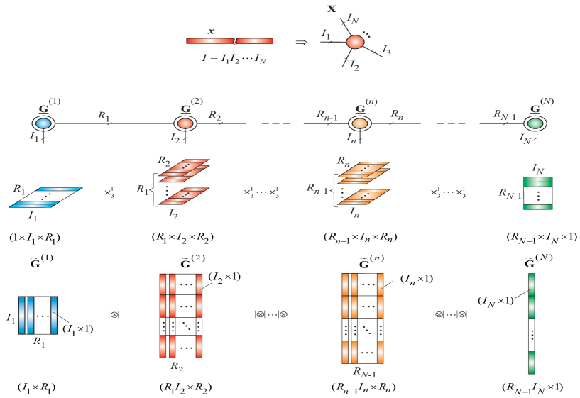
Refer to caption

(b)

Refer to caption
Refer to caption
Figure  20: Example 2 of tensorization and TT decompositions of a huge vector (a) and a matrix (b). TT networks are represented via strong Kronecker products of block matrices.

Since 𝐗𝐗{\bf X} is usually a full rank matrix the straightforward 2N2𝑁2N dimensional exact TT decomposition is inefficient, as it has the rank Rn=INsubscript𝑅𝑛superscript𝐼𝑁R_{n}=I^{N} in the middle of a chain. Therefore, the matrix TT/MPO decompositions employ the index permutation as illustrated in Fig. 20 (b), and can be described in a scalar form as:

xi1,j1,,iN,jNsubscript𝑥subscript𝑖1subscript𝑗1subscript𝑖𝑁subscript𝑗𝑁\displaystyle x_{i_{1},j_{1},\ldots,i_{N},j_{N}} \displaystyle\cong r1=1R1r2=1R2rN1=1RN1g 1,i1,j1,r1(1)gr1,i2,j2,r2(2)superscriptsubscriptsubscript𝑟11subscript𝑅1superscriptsubscriptsubscript𝑟21subscript𝑅2superscriptsubscriptsubscript𝑟𝑁11subscript𝑅𝑁1subscriptsuperscript𝑔11subscript𝑖1subscript𝑗1subscript𝑟1subscriptsuperscript𝑔2subscript𝑟1subscript𝑖2subscript𝑗2subscript𝑟2\displaystyle\sum_{r_{1}=1}^{R_{1}}\sum_{r_{2}=1}^{R_{2}}\cdots\sum_{r_{N-1}=1}^{R_{N-1}}g^{(1)}_{\,1,i_{1},j_{1},r_{1}}\;g^{(2)}_{r_{1},i_{2},j_{2},r_{2}} (17)
\displaystyle\cdots grN2,iN1,jN1,rN1(N1)grN1,iN,jN,1(N).subscriptsuperscript𝑔𝑁1subscript𝑟𝑁2subscript𝑖𝑁1subscript𝑗𝑁1subscript𝑟𝑁1subscriptsuperscript𝑔𝑁subscript𝑟𝑁1subscript𝑖𝑁subscript𝑗𝑁1\displaystyle g^{(N-1)}_{r_{N-2},i_{N-1},j_{N-1},r_{N-1}}\;g^{(N)}_{r_{N-1},i_{N},j_{N},1}.

or equivalently using slice representation

xi1,j1,,iN,jN𝐆(1)(i1,j1)𝐆(2)(i2,j2)𝐆(N)(iN,jN),subscript𝑥subscript𝑖1subscript𝑗1subscript𝑖𝑁subscript𝑗𝑁superscript𝐆1subscript𝑖1subscript𝑗1superscript𝐆2subscript𝑖2subscript𝑗2superscript𝐆𝑁subscript𝑖𝑁subscript𝑗𝑁x_{i_{1},j_{1},\ldots,i_{N},j_{N}}\cong{\bf G}^{(1)}(i_{1},j_{1})\;{\bf G}^{(2)}(i_{2},j_{2})\cdots{\bf G}^{(N)}(i_{N},j_{N}),\\ (18)

where 𝐆(n)(in,jn)𝐆¯(n)(:,in,jn,:)superscript𝐆𝑛subscript𝑖𝑛subscript𝑗𝑛superscript¯𝐆𝑛:subscript𝑖𝑛subscript𝑗𝑛:{\bf G}^{(n)}(i_{n},j_{n})\cong\underline{{\bf G}}^{(n)}(:,\,i_{n},j_{n},\,:) are slices of the cores 𝐆¯(n)Rn1×In×Jn×Rnsuperscript¯𝐆𝑛superscriptsubscript𝑅𝑛1subscript𝐼𝑛subscript𝐽𝑛subscript𝑅𝑛\underline{{\bf G}}^{(n)}\in\mathbb{R}^{R_{n-1}\times I_{n}\times J_{n}\times R_{n}}

However, the TT/MPO model for an 2N2𝑁2Nth-order tensor 𝐗¯I1×J1×IN×JN¯𝐗superscriptsubscript𝐼1subscript𝐽1subscript𝐼𝑁subscript𝐽𝑁\underline{{\bf X}}\in\mathbb{R}^{I_{1}\times J_{1}\times\cdots I_{N}\times J_{N}} can be described mathematically and graphically, in more elegant global and compact forms666i.e., not for each individual entry of a tensor.(see also Table III for detailed and comparative descriptions):

A) In the tensor compact form using multilinear products

𝐗¯¯𝐗\displaystyle\underline{{\bf X}} \displaystyle\cong 𝐆¯(1)×41𝐆¯(2)×41×41𝐆¯(N)superscriptsubscript41superscriptsubscript41superscriptsubscript41superscript¯𝐆1superscript¯𝐆2superscript¯𝐆𝑁\displaystyle\underline{{\bf G}}^{(1)}\;\times_{4}^{1}\;\underline{{\bf G}}^{(2)}\;\times_{4}^{1}\;\cdots\times_{4}^{1}\;\underline{{\bf G}}^{(N)} (19)
=\displaystyle= 𝐆¯(1),𝐆¯(2),,𝐆¯(N),superscript¯𝐆1superscript¯𝐆2superscript¯𝐆𝑁\displaystyle\llbracket\underline{{\bf G}}^{(1)},\underline{{\bf G}}^{(2)},\dots,\underline{{\bf G}}^{(N)}\rrbracket,

where the cores are defined as 𝐆¯(n)Rn1×In×Jn×Rnsuperscript¯𝐆𝑛superscriptsubscript𝑅𝑛1subscript𝐼𝑛subscript𝐽𝑛subscript𝑅𝑛\underline{{\bf G}}^{(n)}\in\mathbb{R}^{R_{n-1}\times I_{n}\times J_{n}\times R_{n}}, with R0=RN=1subscript𝑅0subscript𝑅𝑁1R_{0}=R_{N}=1, (n=1,2,,N𝑛12𝑁n=1,2,\ldots,N).

B) In the block matrix form using the strong Kronecker products:

𝐗𝐆~(1)||𝐆~(2)||||𝐆~(N),{\bf X}\cong\widetilde{\bf G}^{(1)}\;|\otimes|\;\widetilde{\bf G}^{(2)}\;|\otimes|\cdots\;|\otimes|\;\widetilde{\bf G}^{(N)},\\ (20)

where 𝐗=𝐗(i1,i2,,iN¯;j1,j2,,jN¯)I1I2IN×J1J2JN𝐗subscript𝐗¯subscript𝑖1subscript𝑖2subscript𝑖𝑁¯subscript𝑗1subscript𝑗2subscript𝑗𝑁superscriptsubscript𝐼1subscript𝐼2subscript𝐼𝑁subscript𝐽1subscript𝐽2subscript𝐽𝑁{\bf X}={\bf X}_{(\overline{i_{1},i_{2},\ldots,i_{N}}\;;\;\overline{j_{1},j_{2},\ldots,j_{N}})}\in\mathbb{R}^{I_{1}I_{2}\cdots I_{N}\times J_{1}J_{2}\cdots J_{N}} is unfolding matrix of 𝐗¯¯𝐗\underline{{\bf X}} and 𝐆~(n)Rn1In×RnJnsuperscript~𝐆𝑛superscriptsubscript𝑅𝑛1subscript𝐼𝑛subscript𝑅𝑛subscript𝐽𝑛\widetilde{\bf G}^{(n)}\in\mathbb{R}^{R_{n-1}I_{n}\times R_{n}J_{n}} are block matrices with blocks 𝐆rn1,rn(n)In×Jnsubscriptsuperscript𝐆𝑛subscript𝑟𝑛1subscript𝑟𝑛superscriptsubscript𝐼𝑛subscript𝐽𝑛{\bf G}^{(n)}_{r_{n-1},r_{n}}\in\mathbb{R}^{I_{n}\times J_{n}} and the number of blocks Rn1×Rnsubscript𝑅𝑛1subscript𝑅𝑛R_{n-1}\times R_{n}. In the special case, when ranks of the TT/MPO Rn=1,nsubscript𝑅𝑛1for-all𝑛R_{n}=1,\;\forall n the strong Kronecker products simplify to the standard Kronecker products.

VI Basic Operations in TT Formats

Using the compact representations of the TT/MPS and TT/MPO decompositions described in the previous section, we can perform easily basic mathematical operations (e.g., matrix by vector and matrix by matrix multiplications) using block matrices. For example, the large-scale matrix equation

𝐀𝐱=𝒚,𝐀𝐱𝒚\displaystyle{\bf A}{\bf x}=\mbox{\boldmath$y$}, (21)

where 𝐀I×J𝐀superscript𝐼𝐽{\bf A}\in\mathbb{R}^{I\times J}, 𝐱J𝐱superscript𝐽\;\;{\bf x}\in\mathbb{R}^{J} and 𝒚I𝒚superscript𝐼\mbox{\boldmath$y$}\in\mathbb{R}^{I} can be represented in TT format (after performing suitable tensorization of the matrix and vectors), as shown in Fig 21 (a), with I=I1I2IN𝐼subscript𝐼1subscript𝐼2subscript𝐼𝑁I=I_{1}I_{2}\cdots I_{N} and J=J1J2JN𝐽subscript𝐽1subscript𝐽2subscript𝐽𝑁J=J_{1}J_{2}\cdots J_{N}, and the cores defined as

𝐀¯(n)Pn1×In×Jn×Pnsuperscript¯𝐀𝑛superscriptsubscript𝑃𝑛1subscript𝐼𝑛subscript𝐽𝑛subscript𝑃𝑛\displaystyle\underline{{\bf A}}^{(n)}\in\mathbb{R}^{P_{n-1}\times I_{n}\times J_{n}\times P_{n}}
𝐗¯(n)Rn1×Jn×Rnsuperscript¯𝐗𝑛superscriptsubscript𝑅𝑛1subscript𝐽𝑛subscript𝑅𝑛\displaystyle\underline{{\bf X}}^{(n)}\in\mathbb{R}^{R_{n-1}\times J_{n}\times R_{n}}
𝐘¯(n)Qn1×In×Qn.superscript¯𝐘𝑛superscriptsubscript𝑄𝑛1subscript𝐼𝑛subscript𝑄𝑛\displaystyle\underline{{\bf Y}}^{(n)}\in\mathbb{R}^{Q_{n-1}\times I_{n}\times Q_{n}}.

By representing the entries of the matrix 𝐀𝐀{\bf A} and vectors 𝐱𝐱{\bf x} and 𝒚𝒚y by outer products as

𝐀¯¯𝐀\displaystyle\underline{{\bf A}} =\displaystyle= p1,p2,,pN1=1P1,P2,,PN1𝐀 1,p1(1)𝐀p1,p2(2)𝐀pN1,1(N)superscriptsubscriptsubscript𝑝1subscript𝑝2subscript𝑝𝑁11subscript𝑃1subscript𝑃2subscript𝑃𝑁1subscriptsuperscript𝐀11subscript𝑝1subscriptsuperscript𝐀2subscript𝑝1subscript𝑝2subscriptsuperscript𝐀𝑁subscript𝑝𝑁11\displaystyle\displaystyle{\sum_{p_{1},p_{2},\ldots,p_{N-1}=1}^{P_{1},P_{2},\ldots,P_{N-1}}}\;\;{\bf A}^{(1)}_{\;1,p_{1}}\;\circ\;{\bf A}^{(2)}_{\;p_{1},p_{2}}\circ\cdots\circ\;{\bf A}^{(N)}_{\;p_{N-1},1}
𝐗¯¯𝐗\displaystyle\underline{{\bf X}} =\displaystyle= r1,r2,,rN1=1R1,R2,,RN1𝐱r1(1)𝐱r1,r2(2)𝐱rN1(N)superscriptsubscriptsubscript𝑟1subscript𝑟2subscript𝑟𝑁11subscript𝑅1subscript𝑅2subscript𝑅𝑁1subscriptsuperscript𝐱1subscript𝑟1subscriptsuperscript𝐱2subscript𝑟1subscript𝑟2subscriptsuperscript𝐱𝑁subscript𝑟𝑁1\displaystyle\displaystyle{\sum_{r_{1},r_{2},\ldots,r_{N-1}=1}^{R_{1},R_{2},\ldots,R_{N-1}}}\;\;{\bf x}^{(1)}_{\;r_{1}}\;\circ\;{\bf x}^{(2)}_{\;r_{1},r_{2}}\circ\cdots\circ\;{\bf x}^{(N)}_{\;r_{N-1}} (22)
𝐘¯¯𝐘\displaystyle\underline{{\bf Y}} =\displaystyle= q1,q2,,qN1=1Q1,Q2,,QN1𝒚q1(1)𝒚q1,q2(2)𝒚qN1(N),superscriptsubscriptsubscript𝑞1subscript𝑞2subscript𝑞𝑁11subscript𝑄1subscript𝑄2subscript𝑄𝑁1subscriptsuperscript𝒚1subscript𝑞1subscriptsuperscript𝒚2subscript𝑞1subscript𝑞2subscriptsuperscript𝒚𝑁subscript𝑞𝑁1\displaystyle\displaystyle{\sum_{q_{1},q_{2},\ldots,q_{N-1}=1}^{Q_{1},Q_{2},\ldots,Q_{N-1}}}\;\;\mbox{\boldmath$y$}^{(1)}_{\;q_{1}}\;\circ\;\mbox{\boldmath$y$}^{(2)}_{\;q_{1},q_{2}}\circ\cdots\circ\;\mbox{\boldmath$y$}^{(N)}_{\;q_{N-1}},

we can establish the following formulas:

𝒚qn1,qn(n)subscriptsuperscript𝒚𝑛subscript𝑞𝑛1subscript𝑞𝑛\displaystyle\mbox{\boldmath$y$}^{(n)}_{q_{n-1},q_{n}} =\displaystyle= 𝒚rn1pn1¯,rnpn¯(n)subscriptsuperscript𝒚𝑛¯subscript𝑟𝑛1subscript𝑝𝑛1¯subscript𝑟𝑛subscript𝑝𝑛\displaystyle\mbox{\boldmath$y$}^{(n)}_{\overline{r_{n-1}p_{n-1}},\;\overline{r_{n}p_{n}}}
=\displaystyle= 𝐀pn1,pn(n)𝐱rn1,rn(n)In,subscriptsuperscript𝐀𝑛subscript𝑝𝑛1subscript𝑝𝑛subscriptsuperscript𝐱𝑛subscript𝑟𝑛1subscript𝑟𝑛superscriptsubscript𝐼𝑛\displaystyle{\bf A}^{(n)}_{p_{n-1},p_{n}}\;{\bf x}^{(n)}_{r_{n-1},r_{n}}\in\mathbb{R}^{I_{n}},

with Qn=PnRnsubscript𝑄𝑛subscript𝑃𝑛subscript𝑅𝑛Q_{n}=P_{n}R_{n} for n=1,2,,N𝑛12𝑁n=1,2,\ldots,N.

On the other hand, by representing the matrix 𝐀𝐀{\bf A} and vectors 𝐱𝐱{\bf x}, 𝒚𝒚y via the strong Kronecker products:

𝐀𝐀\displaystyle{\bf A} =\displaystyle= 𝐀~(1)||𝐀~(2)||||𝐀~(N)\displaystyle\tilde{\bf A}^{(1)}|\otimes|\tilde{\bf A}^{(2)}|\otimes|\cdots|\otimes|\tilde{\bf A}^{(N)}
𝐱𝐱\displaystyle{\bf x} =\displaystyle= 𝐗~(1)||𝐗~(2)||||𝐗~(N)\displaystyle\tilde{\bf X}^{(1)}|\otimes|\tilde{\bf X}^{(2)}|\otimes|\cdots|\otimes|\tilde{\bf X}^{(N)} (24)
𝒚𝒚y =\displaystyle= 𝐘~(1)||𝐘~(2)||||𝐘~(N),\displaystyle\tilde{\bf Y}^{(1)}|\otimes|\tilde{\bf Y}^{(2)}|\otimes|\cdots|\otimes|\tilde{\bf Y}^{(N)},

with 𝐀~(n)Pn1In×JnPn,𝐗~(n)Rn1Jn×Rnformulae-sequencesuperscript~𝐀𝑛superscriptsubscript𝑃𝑛1subscript𝐼𝑛subscript𝐽𝑛subscript𝑃𝑛superscript~𝐗𝑛superscriptsubscript𝑅𝑛1subscript𝐽𝑛subscript𝑅𝑛\tilde{\bf A}^{(n)}\in\mathbb{R}^{P_{n-1}I_{n}\times J_{n}P_{n}},\;\;\tilde{\bf X}^{(n)}\in\mathbb{R}^{R_{n-1}J_{n}\times R_{n}} and 𝐘~(n)Qn1In×Qnsuperscript~𝐘𝑛superscriptsubscript𝑄𝑛1subscript𝐼𝑛subscript𝑄𝑛\tilde{\bf Y}^{(n)}\in\mathbb{R}^{Q_{n-1}I_{n}\times Q_{n}}, we can easily establish a simple relationship

𝐘~(n)superscript~𝐘𝑛\displaystyle\tilde{\bf Y}^{(n)} =\displaystyle= 𝐀~(n)||𝐗~(n)Rn1Pn1In×RnPn,\displaystyle\tilde{\bf A}^{(n)}|\cdot|\tilde{\bf X}^{(n)}\in\mathbb{R}^{R_{n-1}P_{n-1}I_{n}\times R_{n}P_{n}}, (25)
n=1,2,,N,𝑛12𝑁\displaystyle n=1,2,\ldots,N,

where operator |||\cdot| means the AC product of two block matrices.

In general, the AC product of a block matrix 𝐀(n)Pn1In×PnJnsuperscript𝐀𝑛superscriptsubscript𝑃𝑛1subscript𝐼𝑛subscript𝑃𝑛subscript𝐽𝑛{\bf A}^{(n)}\in\mathbb{R}^{P_{n-1}I_{n}\times P_{n}J_{n}} (with blocks 𝐀pn1,pn(n)In×Jnsubscriptsuperscript𝐀𝑛subscript𝑝𝑛1subscript𝑝𝑛superscriptsubscript𝐼𝑛subscript𝐽𝑛{\bf A}^{(n)}_{p_{n-1},p_{n}}\in\mathbb{R}^{I_{n}\times J_{n}}) and a block matrix 𝐁(n)Rn1Jn×RnKnsuperscript𝐁𝑛superscriptsubscript𝑅𝑛1subscript𝐽𝑛subscript𝑅𝑛subscript𝐾𝑛{\bf B}^{(n)}\in\mathbb{R}^{R_{n-1}J_{n}\times R_{n}K_{n}} (with blocks 𝐁rn1,rn(n)Jn×Knsubscriptsuperscript𝐁𝑛subscript𝑟𝑛1subscript𝑟𝑛superscriptsubscript𝐽𝑛subscript𝐾𝑛{\bf B}^{(n)}_{r_{n-1},r_{n}}\in\mathbb{R}^{J_{n}\times K_{n}}) is defined as a block matrix 𝐂(n)=𝐀(n)||𝐁(n)Qn1In×QnKn{\bf C}^{(n)}={\bf A}^{(n)}|\cdot|{\bf B}^{(n)}\in\mathbb{R}^{Q_{n-1}I_{n}\times Q_{n}K_{n}} (with blocks 𝐂qn1,qn(n)=𝐀pn1,pn(n)𝐁rn1,rn(n)In×Knsubscriptsuperscript𝐂𝑛subscript𝑞𝑛1subscript𝑞𝑛subscriptsuperscript𝐀𝑛subscript𝑝𝑛1subscript𝑝𝑛subscriptsuperscript𝐁𝑛subscript𝑟𝑛1subscript𝑟𝑛superscriptsubscript𝐼𝑛subscript𝐾𝑛{\bf C}^{(n)}_{q_{n-1},q_{n}}={\bf A}^{(n)}_{p_{n-1},p_{n}}{\bf B}^{(n)}_{r_{n-1},r_{n}}\in\mathbb{R}^{I_{n}\times K_{n}} as illustrated in Fig. 22.

The AC product of two block matrices is similar to the Tracy-Singh product but the Kronecker product for block matrices is replaced by the ordinary products matrix-by-matrix.

(a)
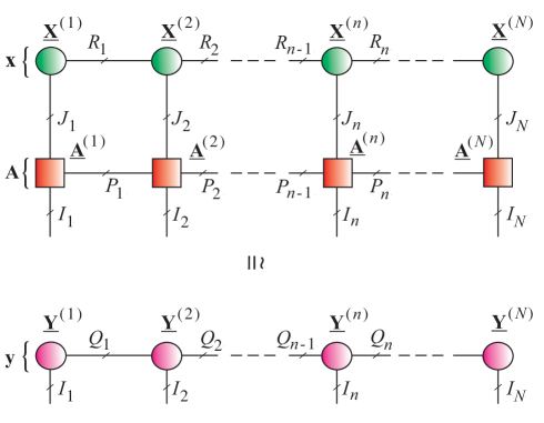
Refer to caption
(b)
Refer to caption

Figure  21: Distributed representation of matrix equations (a) 𝐀𝐱=𝒚𝐀𝐱𝒚{\bf A}{\bf x}=\mbox{\boldmath$y$} and (b) 𝐀𝐗=𝐘𝐀𝐗𝐘{\bf A}{\bf X}={\bf Y} in TT formats.
Refer to caption
Figure  22: Graphical illustration of the AC product for two block matrices.

In a similar way, we can represent in TT format a matrix equation

𝐘𝐀𝐗=𝐀𝐁T,𝐘𝐀𝐗superscript𝐀𝐁𝑇\displaystyle{\bf Y}\cong{\bf A}{\bf X}={\bf A}{\bf B}^{T}, (26)

where 𝐀I×J𝐀superscript𝐼𝐽{\bf A}\in\mathbb{R}^{I\times J}, 𝐗=𝐁TJ×K𝐗superscript𝐁𝑇superscript𝐽𝐾\;\;{\bf X}={\bf B}^{T}\in\mathbb{R}^{J\times K} and 𝐘I×K𝐘superscript𝐼𝐾{\bf Y}\in\mathbb{R}^{I\times K} as shown in Fig 21 (b), with I=I1I2IN𝐼subscript𝐼1subscript𝐼2subscript𝐼𝑁I=I_{1}I_{2}\cdots I_{N}, J=J1J2JN𝐽subscript𝐽1subscript𝐽2subscript𝐽𝑁J=J_{1}J_{2}\cdots J_{N} and K=K1K2KN𝐾subscript𝐾1subscript𝐾2subscript𝐾𝑁K=K_{1}K_{2}\cdots K_{N} with the cores defined as

𝐀¯(n)Pn1×In×Pn×Jnsuperscript¯𝐀𝑛superscriptsubscript𝑃𝑛1subscript𝐼𝑛subscript𝑃𝑛subscript𝐽𝑛\displaystyle\underline{{\bf A}}^{(n)}\in\mathbb{R}^{P_{n-1}\times I_{n}\times P_{n}\times J_{n}}
𝐗¯(n)Rn1×Jn×Rn×Knsuperscript¯𝐗𝑛superscriptsubscript𝑅𝑛1subscript𝐽𝑛subscript𝑅𝑛subscript𝐾𝑛\displaystyle\underline{{\bf X}}^{(n)}\in\mathbb{R}^{R_{n-1}\times J_{n}\times R_{n}\times K_{n}}
𝐘¯(n)Qn1×In×Qn×Kn.superscript¯𝐘𝑛superscriptsubscript𝑄𝑛1subscript𝐼𝑛subscript𝑄𝑛subscript𝐾𝑛\displaystyle\underline{{\bf Y}}^{(n)}\in\mathbb{R}^{Q_{n-1}\times I_{n}\times Q_{n}\times K_{n}}.

It can be proved that by assuming that matrices: 𝐀I×J𝐀superscript𝐼𝐽{\bf A}\in\mathbb{R}^{I\times J} and 𝐗J×K𝐗superscript𝐽𝐾{\bf X}\in\mathbb{R}^{J\times K} are represented in TT formats and expressed via the strong Kronecker product of block matrices as: 𝐀=𝐀~(1)||𝐀~(2)||||𝐀~(N){\bf A}=\tilde{\bf A}^{(1)}|\otimes|\tilde{\bf A}^{(2)}|\otimes|\cdots|\otimes|\tilde{\bf A}^{(N)} and 𝐗=𝐗~(1)||𝐗~(2)||||𝐗~(N){\bf X}=\tilde{\bf X}^{(1)}|\otimes|\tilde{\bf X}^{(2)}|\otimes|\cdots|\otimes|\tilde{\bf X}^{(N)}, with 𝐀~(n)Pn1In×JnPnsuperscript~𝐀𝑛superscriptsubscript𝑃𝑛1subscript𝐼𝑛subscript𝐽𝑛subscript𝑃𝑛\tilde{\bf A}^{(n)}\in\mathbb{R}^{P_{n-1}I_{n}\times J_{n}P_{n}} and 𝐗~(n)Rn1Jn×KnRnsuperscript~𝐗𝑛superscriptsubscript𝑅𝑛1subscript𝐽𝑛subscript𝐾𝑛subscript𝑅𝑛\tilde{\bf X}^{(n)}\in\mathbb{R}^{R_{n-1}J_{n}\times K_{n}R_{n}}, respectively, then the matrix 𝐘=𝐀𝐗𝐘𝐀𝐗{\bf Y}={\bf A}{\bf X} can be expressed in TT format via the strong Kronecker products: 𝐘=𝐘~(1)||𝐘~(2)||||𝐘~(N){\bf Y}=\tilde{\bf Y}^{(1)}|\otimes|\tilde{\bf Y}^{(2)}|\otimes|\cdots|\otimes|\tilde{\bf Y}^{(N)}, where 𝐘~(n)=𝐀~(n)||𝐗~(n)Qn1In×KnQn\tilde{\bf Y}^{(n)}=\tilde{\bf A}^{(n)}|\cdot|\tilde{\bf X}^{(n)}\in\mathbb{R}^{Q_{n-1}I_{n}\times K_{n}Q_{n}}, (n=1,2,,N)𝑛12𝑁(n=1,2,\ldots,N), with blocks 𝐘~qn1,qn(n)=𝐀~pn1,pn(n)𝐗~rn1,rn(n)superscriptsubscript~𝐘subscript𝑞𝑛1subscript𝑞𝑛𝑛subscriptsuperscript~𝐀𝑛subscript𝑝𝑛1subscript𝑝𝑛subscriptsuperscript~𝐗𝑛subscript𝑟𝑛1subscript𝑟𝑛\tilde{\bf Y}_{q_{n-1},q_{n}}^{(n)}=\tilde{\bf A}^{(n)}_{p_{n-1},p_{n}}\tilde{\bf X}^{(n)}_{r_{n-1},r_{n}}, where Qn=RnPn,nsubscript𝑄𝑛subscript𝑅𝑛subscript𝑃𝑛for-all𝑛Q_{n}=R_{n}P_{n},\;\;\forall n.

The above operation assumes precise contraction of cores. However, an exact contraction of core tensors for very large scale data is impossible, and the choice of the approximating procedure determines the efficiency and accuracy of algorithms implemented for specific computational or optimization problems [27]. In other words, contraction operations as matrix-by-vector or matrix-by-matrix products TT ranks grows and the TT ranks could become excessively large and therefore truncation (called also recompression) or low-rank matrix approximations are needed. In the truncation procedure (usually, performed via QR/SVD or CUR) the core tensors 𝐆¯(n)superscript¯𝐆𝑛\underline{{\bf G}}^{(n)} are approximated by other core tensors with minimal possible TT-ranks with desired prescribed accuracy [40].

VII Tensor Train (TT/MPS) Splitting

In practical applications it is very useful and efficient to divide a TT decomposition, representing a tensor 𝐗¯=𝐆¯(1),𝐆¯(2),,𝐆¯(N)I1×I2××IN¯𝐗superscript¯𝐆1superscript¯𝐆2superscript¯𝐆𝑁superscriptsubscript𝐼1subscript𝐼2subscript𝐼𝑁\underline{{\bf X}}=\llbracket\underline{{\bf G}}^{(1)},\underline{{\bf G}}^{(2)},\ldots,\underline{{\bf G}}^{(N)}\rrbracket\in\mathbb{R}^{I_{1}\times I_{2}\times\cdots\times I_{N}}, into subtrains as illustrated in Fig. 23.

VII-A Extraction of a single core

For this purpose, we define subtrains as follows

𝐆¯<n=𝐆¯(1),𝐆¯(2),,𝐆¯(n1)I1×I2××In1×Rn1superscript¯𝐆absent𝑛superscript¯𝐆1superscript¯𝐆2superscript¯𝐆𝑛1superscriptsubscript𝐼1subscript𝐼2subscript𝐼𝑛1subscript𝑅𝑛1\underline{{\bf G}}^{<n}=\llbracket\underline{{\bf G}}^{(1)},\underline{{\bf G}}^{(2)},\ldots,\underline{{\bf G}}^{(n-1)}\rrbracket\in\mathbb{R}^{I_{1}\times I_{2}\times\cdots\times I_{n-1}\times R_{n-1}}\\ (27)
𝐆¯>n=𝐆¯(n+1),𝐆¯(n+2),,𝐆¯(N)Rn×In+1××INsuperscript¯𝐆absent𝑛superscript¯𝐆𝑛1superscript¯𝐆𝑛2superscript¯𝐆𝑁superscriptsubscript𝑅𝑛subscript𝐼𝑛1subscript𝐼𝑁\underline{{\bf G}}^{>n}=\llbracket\underline{{\bf G}}^{(n+1)},\underline{{\bf G}}^{(n+2)},\ldots,\underline{{\bf G}}^{(N)}\rrbracket\in\mathbb{R}^{R_{n}\times I_{n+1}\times\cdots\times I_{N}}\\ (28)

with corresponding unfolding matrices called interface matrices:

𝐆(n)<nRn1×I1I2In1subscriptsuperscript𝐆absent𝑛𝑛superscriptsubscript𝑅𝑛1subscript𝐼1subscript𝐼2subscript𝐼𝑛1\displaystyle{\bf G}^{<n}_{(n)}\in\mathbb{R}^{R_{n-1}\times I_{1}I_{2}\cdots I_{n-1}} (29)
𝐆(1)>nRn×In+1INsubscriptsuperscript𝐆absent𝑛1superscriptsubscript𝑅𝑛subscript𝐼𝑛1subscript𝐼𝑁\displaystyle{\bf G}^{>n}_{(1)}\in\mathbb{R}^{R_{n}\times I_{n+1}\cdots I_{N}} (30)

(a)
Refer to caption
(b)
Refer to caption

Figure  23: Extraction of a single core. (a) Graphical representation and notations of vector tensor train and subtrains. (b) Graphical illustration of the equation expressed via interface matrices or a frame matrix (see Eqs. (31) and (32)).

Using basic multilinear algebra, we can construct a set of linear equations referred to as the frame equation:

𝐱=𝐆n𝐠(n),n=1,2,,N,formulae-sequence𝐱subscript𝐆absent𝑛superscript𝐠𝑛𝑛12𝑁\displaystyle{\bf x}={\bf G}_{\neq\,n}\;{\bf g}^{(n)},\qquad n=1,2,\ldots,N, (31)

where 𝐱=vec(𝐗¯)I1I2IN𝐱𝑣𝑒𝑐¯𝐗superscriptsubscript𝐼1subscript𝐼2subscript𝐼𝑁{\bf x}=vec(\underline{{\bf X}})\in\mathbb{R}^{I_{1}I_{2}\cdots I_{N}}, 𝐠(n)=vec(𝐆¯(n))Rn1InRnsuperscript𝐠𝑛𝑣𝑒𝑐superscript¯𝐆𝑛superscriptsubscript𝑅𝑛1subscript𝐼𝑛subscript𝑅𝑛\;\;{\bf g}^{(n)}=vec(\underline{{\bf G}}^{(n)})\in\mathbb{R}^{R_{n-1}I_{n}R_{n}} and a tall-and-skinny matrix, called the frame matrix, formulated as

𝐆n=(𝐆(n)<n)T𝐈In(𝐆(1)>n)TI1I2IN×Rn1InRn.subscript𝐆absent𝑛tensor-productsuperscriptsubscriptsuperscript𝐆absent𝑛𝑛𝑇subscript𝐈subscript𝐼𝑛superscriptsubscriptsuperscript𝐆absent𝑛1𝑇superscriptsubscript𝐼1subscript𝐼2subscript𝐼𝑁subscript𝑅𝑛1subscript𝐼𝑛subscript𝑅𝑛{\bf G}_{\neq\,n}=({\bf G}^{<n}_{(n)})^{T}\otimes{\bf I}_{I_{n}}\otimes({\bf G}^{>n}_{(1)})^{T}\in\mathbb{R}^{I_{1}I_{2}\cdots I_{N}\times R_{n-1}I_{n}R_{n}}.\\ (32)

The frame and interface matrices help to show a very important property of TT, – TT is linear with respect to each core 𝐆(n)superscript𝐆𝑛{\bf G}^{(n)} in the vectorized form [40].

VII-B Extraction of two cores for two–sided DMRG

In a similar way, we can formulate equations for the 2-sided DMRG, where we extract block of two consecutive cores (see Fig. 24):

𝐱=𝐆n,n+1𝐠(n,n+1),n=1,2,,N1,formulae-sequence𝐱subscript𝐆absent𝑛𝑛1superscript𝐠𝑛𝑛1𝑛12𝑁1{\bf x}={\bf G}_{\neq\,n,n+1}\;{\bf g}^{(n,n+1)},\;\;n=1,2,\ldots,N-1,\\ (33)

where the frame (tall-and-skinny) matrix is formulated as

𝐆n,n+1subscript𝐆absent𝑛𝑛1\displaystyle{\bf G}_{\neq\,n,n+1} =\displaystyle= (𝐆(n)<n)T𝐈In𝐈In+1(𝐆(1)>n+1)Ttensor-productsuperscriptsubscriptsuperscript𝐆absent𝑛𝑛𝑇subscript𝐈subscript𝐼𝑛subscript𝐈subscript𝐼𝑛1superscriptsubscriptsuperscript𝐆absent𝑛11𝑇\displaystyle({\bf G}^{<n}_{(n)})^{T}\;\otimes\;{\bf I}_{I_{n}}\;\otimes{\bf I}_{I_{n+1}}\otimes\;({\bf G}^{>n+1}_{(1)})^{T} (34)
\displaystyle\in I1I2IN×Rn1InIn+1Rn+1superscriptsubscript𝐼1subscript𝐼2subscript𝐼𝑁subscript𝑅𝑛1subscript𝐼𝑛subscript𝐼𝑛1subscript𝑅𝑛1\displaystyle\mathbb{R}^{I_{1}I_{2}\cdots I_{N}\times R_{n-1}I_{n}I_{n+1}R_{n+1}}

and 𝐠(n,n+1)=vec[𝐆(3)(n)T𝐆(1)(n+1)]=vec(𝐆¯(n,n+1))Rn1InIn+1Rn+1superscript𝐠𝑛𝑛1𝑣𝑒𝑐delimited-[]subscriptsuperscript𝐆𝑛𝑇3subscriptsuperscript𝐆𝑛11𝑣𝑒𝑐superscript¯𝐆𝑛𝑛1superscriptsubscript𝑅𝑛1subscript𝐼𝑛subscript𝐼𝑛1subscript𝑅𝑛1{\bf g}^{(n,n+1)}=vec[{\bf G}^{(n)\;T}_{(3)}{\bf G}^{(n+1)}_{(1)}]=vec(\underline{{\bf G}}^{(n,n+1)})\in\mathbb{R}^{R_{n-1}I_{n}I_{n+1}R_{n+1}} for n=1,2,,N1𝑛12𝑁1n=1,2,\ldots,N-1.

Simple matrix manipulations give the following useful relationships [13]:

𝐗(n)subscript𝐗𝑛\displaystyle{\bf X}_{(n)} =\displaystyle= 𝐆(n)(n)(𝐆(n)<n𝐆(1)>n),subscriptsuperscript𝐆𝑛𝑛tensor-productsubscriptsuperscript𝐆absent𝑛𝑛superscriptsubscript𝐆1absent𝑛\displaystyle{\bf G}^{(n)}_{(n)}\;({\bf G}^{<n}_{(n)}\otimes{\bf G}_{(1)}^{>n}), (35)
𝐆n+1subscript𝐆absent𝑛1\displaystyle{\bf G}_{\neq\;n+1} =\displaystyle= 𝐆n,n+1(𝐈Rn+1In+1𝐆(3)(n)T).subscript𝐆absent𝑛𝑛1tensor-productsubscript𝐈subscript𝑅𝑛1subscript𝐼𝑛1subscriptsuperscript𝐆𝑛𝑇3\displaystyle{\bf G}_{\neq\;n,n+1}\;({\bf I}_{R_{n+1}I_{n+1}}\otimes\;{\bf G}^{(n)\;T}_{(3)}). (36)

If cores are normalized in a such way that all cores to the left of the currently considered (optimized) core 𝐆¯(n)superscript¯𝐆𝑛\underline{{\bf G}}^{(n)} are left-orthogonal:

𝐆(3)(k)𝐆(3)(k)T=𝐈Rk,k<n,formulae-sequencesuperscriptsubscript𝐆3𝑘superscriptsubscript𝐆3𝑘𝑇subscript𝐈subscript𝑅𝑘𝑘𝑛\displaystyle{\bf G}_{(3)}^{(k)}{\bf G}_{(3)}^{(k)\;T}={\bf I}_{R_{k}},\quad k<n, (37)

and all cores to the right of the 𝐆¯(n)superscript¯𝐆𝑛\underline{{\bf G}}^{(n)} are right-orthogonal, i.e.:

𝐆(1)(p)𝐆(1)(p)T=𝐈Rp1,p>n,formulae-sequencesuperscriptsubscript𝐆1𝑝superscriptsubscript𝐆1𝑝𝑇subscript𝐈subscript𝑅𝑝1𝑝𝑛\displaystyle{\bf G}_{(1)}^{(p)}{\bf G}_{(1)}^{(p)\;T}={\bf I}_{R_{p-1}},\quad p>n, (38)

then the frames matrices have orthogonal columns [67, 68, 69]:

𝐆nT𝐆nsuperscriptsubscript𝐆absent𝑛𝑇subscript𝐆absent𝑛\displaystyle{\bf G}_{\neq\,n}^{T}\;{\bf G}_{\neq\;n} =\displaystyle= 𝐈Rn1InRn,subscript𝐈subscript𝑅𝑛1subscript𝐼𝑛subscript𝑅𝑛\displaystyle{\bf I}_{R_{n-1}I_{n}R_{n}}, (39)
𝐆n,n+1T𝐆n,n+1superscriptsubscript𝐆absent𝑛𝑛1𝑇subscript𝐆absent𝑛𝑛1\displaystyle{\bf G}_{\neq\,n,n+1}^{T}\;{\bf G}_{\neq\,n,n+1} =\displaystyle= 𝐈Rn1InIn+1Rn+1.subscript𝐈subscript𝑅𝑛1subscript𝐼𝑛subscript𝐼𝑛1subscript𝑅𝑛1\displaystyle{\bf I}_{R_{n-1}I_{n}I_{n+1}R_{n+1}}. (40)

Orthogonalization of cores is usually performed by the QR/SVD algorithm [40] (see Section VIII for detail).

(a)
Refer to caption
(b)
Refer to caption

Figure  24: Extraction of two cores: (a) Graphical representation of the tensor train and subtrains. (b) Graphical illustration of the frame equation (see Eqs. (33) and (34)).

VIII Application of TT Decompositions to Large-Scale Optimization Problems

For extremely large-scale problems, due to curse of dimensionality, most computation and optimization problems (such as solving eigenvalue problems, SVD, sparse PCA, Canonical Correlation Analysis (CCA), system of linear equations) are intractable when using standard numerical methods.

Our goal and objective is to seek for alternative solutions for specific optimization problems in approximative tensor compressed formats. The key idea discussed in this section is to represent huge data in TT formats and to apply some kind of separation of variables [68, 69, 70]. In other words, we approximate involved vectors and matrices by suitable TT networks and convert a large-scale specific optimization problem into a set of much smaller optimization problems.

We next illustrate this approach by considering several fundamental optimization problems for very large-scale data.

VIII-A Computing a Few Extreme Eigenvalues and Eigenvectors for Symmetric EVD in TT Format

In many applications we need to compute extreme (minimum or maximum) eigenvalues and corresponding eigenvectors of a huge structured symmetric matrix. The basic problem we try to solve is the standard symmetric eigenvalue decomposition (EVD), which can be formulated as

𝐀𝐱k=λk𝐱k,(k=1,2,,K),𝐀subscript𝐱𝑘subscript𝜆𝑘subscript𝐱𝑘𝑘12𝐾\displaystyle{\bf A}\;{\bf x}_{k}=\lambda_{k}{\bf x}_{k},\qquad(k=1,2,\ldots,K), (41)

where 𝐱kIsubscript𝐱𝑘superscript𝐼{\bf x}_{k}\in\mathbb{R}^{I} are the orthonormal eigenvectors, λksubscript𝜆𝑘\lambda_{k} are the corresponding eigenvalues of a symmetric matrix 𝐀I×I𝐀superscript𝐼𝐼{\bf A}\in\mathbb{R}^{I\times I} (e.g., a positive-definite covariance matrix of zero-mean signals 𝒚(t)𝒚𝑡\mbox{\boldmath$y$}(t)). Note that (41) can be written in the matrix form as

𝐗T𝐀𝐗=𝚲K,superscript𝐗𝑇𝐀𝐗subscript𝚲𝐾\displaystyle{\bf X}^{T}\,{\bf A}\,{\bf X}=\mbox{\boldmath$\Lambda$}_{K}, (42)

where 𝚲Ksubscript𝚲𝐾\mbox{\boldmath$\Lambda$}_{K} is the diagonal matrix of K smallest or largest eigenvalues (ranked in ascending or descending order, respectively).

VIII-A1 Tensor Network for Computing Single Eigenvalue and Corresponding Eigenvector

Many iterative algorithms for extreme eigenvalue and the corresponding eignevector exploit the Rayleigh quotient (RQ) of the symmetric matrix as a cost function. The Rayleigh quotient R(𝐱)𝑅𝐱R({\bf x}) is defined for 𝐱𝟎𝐱0{\bf x}\neq{\bf 0}, as

J(𝐱)=R(𝐱,𝐀)=𝐱T𝐀𝐱𝐱T𝐱=𝐀𝐱,𝐱𝐱,𝐱,𝐽𝐱𝑅𝐱𝐀superscript𝐱𝑇𝐀𝐱superscript𝐱𝑇𝐱𝐀𝐱𝐱𝐱𝐱\displaystyle J({\bf x})=R({\bf x},{\bf A})=\frac{{\bf x}^{T}{\bf A}{\bf x}}{{\bf x}^{T}{\bf x}}=\frac{\langle{\bf A}{\bf x},{\bf x}\rangle}{\langle{\bf x},{\bf x}\rangle}, (43)

where

λmax=maxR(𝐱,𝐀),λmin=minR(𝐱,𝐀),formulae-sequencesubscript𝜆𝑚𝑎𝑥𝑅𝐱𝐀subscript𝜆𝑚𝑖𝑛𝑅𝐱𝐀\displaystyle\lambda_{max}=\max R({\bf x},{\bf A}),\quad\lambda_{min}=\min R({\bf x},{\bf A}), (44)

where λmaxsubscript𝜆𝑚𝑎𝑥\lambda_{max} and λminsubscript𝜆𝑚𝑖𝑛\lambda_{min} denote respectively largest and smallest eigenvalue of the matrix 𝐀𝐀{\bf A}. More generally, the critical points and critical values of R(𝐱,𝐀)𝑅𝐱𝐀R({\bf x},{\bf A}) are the eigenvectors and eigenvalues of 𝐀𝐀{\bf A}.

If the matrix 𝐀𝐀{\bf A} admits low-rank TT approximation, we can convert large-scale problems into smaller optimization problems by representing the eigenvector 𝐱𝐱{\bf x} and the matrix 𝐀𝐀{\bf A} in TT (MPO/MPS) formats (see also Fig. 25) as:

𝐀¯¯𝐀\displaystyle\underline{{\bf A}} =\displaystyle= 𝐀¯(1),𝐀¯(2),,𝐀¯(N)superscript¯𝐀1superscript¯𝐀2superscript¯𝐀𝑁\displaystyle\llbracket\underline{{\bf A}}^{(1)},\underline{{\bf A}}^{(2)},\ldots,\underline{{\bf A}}^{(N)}\rrbracket
𝐗¯¯𝐗\displaystyle\underline{{\bf X}} =\displaystyle= 𝐗¯(1),𝐗¯(2),,𝐗¯(N)superscript¯𝐗1superscript¯𝐗2superscript¯𝐗𝑁\displaystyle\llbracket\underline{{\bf X}}^{(1)},\underline{{\bf X}}^{(2)},\ldots,\underline{{\bf X}}^{(N)}\rrbracket (45)

and by computing iteratively the frame equation 𝐱=𝐗n𝐱(n)𝐱subscript𝐗absent𝑛superscript𝐱𝑛{\bf x}={\bf X}_{\neq n}\;{\bf x}^{(n)}, (n=1,2,,N)𝑛12𝑁(n=1,2,\ldots,N), with the frame matrices:

𝐗n=(𝐗(n)<n)T𝐈In(𝐗(1)>n)TI1I2IN×Rn1InRn.subscript𝐗absent𝑛tensor-productsuperscriptsubscriptsuperscript𝐗absent𝑛𝑛𝑇subscript𝐈subscript𝐼𝑛superscriptsubscriptsuperscript𝐗absent𝑛1𝑇superscriptsubscript𝐼1subscript𝐼2subscript𝐼𝑁subscript𝑅𝑛1subscript𝐼𝑛subscript𝑅𝑛\displaystyle{\bf X}_{\neq n}=({\bf X}^{<n}_{(n)})^{T}\otimes{\bf I}_{I_{n}}\otimes({\bf X}^{>n}_{(1)})^{T}\in\mathbb{R}^{I_{1}I_{2}\cdots I_{N}\times R_{n-1}I_{n}R_{n}}.

Assuming that cores 𝐗¯(n)superscript¯𝐗𝑛\underline{{\bf X}}^{(n)} are constrained to be left and right orthogonal, we can minimize (or maximize) the RQ as follows:

min𝐱J(𝐱)subscript𝐱𝐽𝐱\displaystyle\min_{{\bf x}}J({\bf x}) =\displaystyle= min𝐱(n)J(𝐗n𝐱(n))subscriptsuperscript𝐱𝑛𝐽subscript𝐗absent𝑛superscript𝐱𝑛\displaystyle\min_{{\bf x}^{(n)}}J({\bf X}_{\neq n}{\bf x}^{(n)})
=\displaystyle= min𝐱(n)𝐀¯(n)𝐱(n),𝐱(n)𝐱(n),𝐱(n),n=1,2,,N,formulae-sequencesubscriptsuperscript𝐱𝑛superscript¯𝐀𝑛superscript𝐱𝑛superscript𝐱𝑛superscript𝐱𝑛superscript𝐱𝑛𝑛12𝑁\displaystyle\min_{{\bf x}^{(n)}}\frac{\langle\bar{\bf A}^{(n)}{\bf x}^{(n)},{\bf x}^{(n)}\rangle}{\langle{\bf x}^{(n)},{\bf x}^{(n)}\rangle},\quad n=1,2,\ldots,N,

where 𝐱(n)=vec(𝐗¯(n))Rn1InRnsuperscript𝐱𝑛𝑣𝑒𝑐superscript¯𝐗𝑛superscriptsubscript𝑅𝑛1subscript𝐼𝑛subscript𝑅𝑛{\bf x}^{(n)}=vec(\underline{{\bf X}}^{(n)})\in\mathbb{R}^{R_{n-1}I_{n}R_{n}} and the matrix 𝐀¯¯𝐀\bar{\bf A}, often called the effective Hamiltonian, and can be expressed as

𝐀¯(n)=(𝐗n)T𝐀𝐗nRn1InRn×Rn1InRnsuperscript¯𝐀𝑛superscriptsubscript𝐗absent𝑛𝑇subscript𝐀𝐗absent𝑛superscriptsubscript𝑅𝑛1subscript𝐼𝑛subscript𝑅𝑛subscript𝑅𝑛1subscript𝐼𝑛subscript𝑅𝑛\displaystyle\bar{\bf A}^{(n)}=({\bf X}_{\neq n})^{T}{\bf A}{\bf X}_{\neq n}\in\mathbb{R}^{R_{n-1}I_{n}R_{n}\times R_{n-1}I_{n}R_{n}} (47)

for n=1,2,,N𝑛12𝑁n=1,2,\ldots,N.

Refer to caption
Figure  25: Computation of a single extreme eigenvalue and the corresponding eigenvector 𝐱I𝐱superscript𝐼{\bf x}\in\mathbb{R}^{I} in the TT format for a symmetric matrix 𝐀I×I𝐀superscript𝐼𝐼{\bf A}\in\mathbb{R}^{I\times I}. The frame matrix maps a TT core into a large vector. The tensor network corresponds to the Rayleigh quotient, with the matrix 𝐀𝐀{\bf A} and vectors 𝐱I𝐱superscript𝐼{\bf x}\in\mathbb{R}^{I} given in the tensor train format with distributed indices I=I1I2IN𝐼subscript𝐼1subscript𝐼2subscript𝐼𝑁I=I_{1}I_{2}\cdots I_{N}. The cores included in the shaded areas form the matrix 𝐀¯(n)superscript¯𝐀𝑛\bar{\bf A}^{(n)} (the effective Hamiltonian), which can computed by sequential core contractions.

Note that the matrices 𝐀¯(n)superscript¯𝐀𝑛\bar{\bf A}^{(n)} are usually much smaller than the original matrix 𝐀𝐀{\bf A} if the TT rank is relatively small, then, the large-scale optimization problem can be converted into a much smaller set of EVDs, i.e., by solving the set of equations:

𝐀¯(n)𝐱(n)=λ𝐱(n),n=1,2,,N.formulae-sequencesuperscript¯𝐀𝑛superscript𝐱𝑛𝜆superscript𝐱𝑛𝑛12𝑁\displaystyle\bar{\bf A}^{(n)}{\bf x}^{(n)}=\lambda{\bf x}^{(n)},\quad n=1,2,\ldots,N. (48)

In practice, we never compute the matrices 𝐀¯(n)superscript¯𝐀𝑛\bar{\bf A}^{(n)} directly by Eq. (47), but iteratively via optimized and approximative contraction of cores of the tensor network as shown in Fig. 26.

(a)

Refer to caption

(b)

Refer to caption
Figure  26: (a) Non-optimal (inefficient) and (b) optimal (efficient) contraction of the TT (MPS/MPO) network.

This is achieved by sweeping through the tensor network in a recursive forward and backward manner and forth through each node. An initial guess for all cores 𝐗¯(n)superscript¯𝐗𝑛\underline{{\bf X}}^{(n)} is first made, and then we sweep through the set of the cores with the index n𝑛n, keeping all other cores fixed and choosing the 𝐗¯(n)superscript¯𝐗𝑛\underline{{\bf X}}^{(n)}, such that the cost function gradually decreases. By repeating such sweeps (from the left to the right and from the right to the left) through the tensor network several times that usually leads to a converged approximation. Note that this sweeping process works in a similar fashion as a self-consistent recursive loops, where we iteratively and gradually improve the solution.

In order to efficiently estimate the matrix 𝐀¯(n)superscript¯𝐀𝑛\bar{\bf A}^{(n)}, we need to compute blocks 𝐋¯<nsuperscript¯𝐋absent𝑛\underline{{\bf L}}^{<n} and 𝐑¯>nsuperscript¯𝐑absent𝑛\underline{{\bf R}}^{>n} (see Fig. 25). However, 𝐋¯<nsuperscript¯𝐋absent𝑛\underline{{\bf L}}^{<n} and 𝐑¯>nsuperscript¯𝐑absent𝑛\underline{{\bf R}}^{>n} can be built iteratively in order to best reuse available information; this involves an optimal arrangement of a tensor network contraction. In a practical implementation of the algorithm the full network contraction is never carried out globally, but we rather look at blocks 𝐋¯nsuperscript¯𝐋𝑛\underline{{\bf L}}^{n} and 𝐑¯>nsuperscript¯𝐑absent𝑛\underline{{\bf R}}^{>n} that are growing and shrinking in size sweeping along the tensor network [49]. In other words, the construction of blocks 𝐋¯<nsuperscript¯𝐋absent𝑛\underline{{\bf L}}^{<n} and 𝐑¯>nsuperscript¯𝐑absent𝑛\underline{{\bf R}}^{>n} is an iterative process in a way that directly matches block growth and shrinkage. If we sweep through the chain from right to left or vice-versa we can build up 𝐋¯<nsuperscript¯𝐋absent𝑛\underline{{\bf L}}^{<n} and 𝐑¯>nsuperscript¯𝐑absent𝑛\underline{{\bf R}}^{>n} iteratively from the previous steps, which is the most efficient way [49]. Furthermore, we can exploit left- and right-orthogonalization of the cores in order to simplify the tensor contraction process [68, 69, 13].

As in any iterative optimization based on gradient descent the cost function can only decrease, however we have no guarantee that a global minimum is achieved. Moreover, for some initial conditions the iteration process can be slow. To alleviate these problems we can exploit double site DMRG, in which we join two neighboring factors (cores), optimize the resulting “supernode” called also “super-core” or “super-block”, and split again the result into separated factors by low-rank matrix factorizations [68, 69, 49, 71].

VIII-A2 Tensor Network for Computing Several Extreme Eigenvalues and Corresponding Eigenvectors for Symmetric Eigenvalue Problem

In a more general case, in order to compute a few, say K𝐾K eigenvectors corresponding to K𝐾K algebraically smallest eigenvalues for a symmetric matrix 𝐀I×I𝐀superscript𝐼𝐼{\bf A}\in\mathbb{R}^{I\times I}, we can employ the following trace minimization problem with orthogonality constraints

min𝐗tr(𝐗T𝐀𝐗),s.t.𝐗T𝐗=𝐈K,subscript𝐗trsuperscript𝐗𝑇𝐀𝐗s.t.superscript𝐗𝑇𝐗subscript𝐈𝐾\displaystyle\min_{{\bf X}}\mathop{\rm tr}\nolimits({\bf X}^{T}{\bf A}{\bf X}),\qquad\mbox{s.t.}\;\;{\bf X}^{T}{\bf X}={\bf I}_{K}, (49)

where 𝐗=[𝐱1,𝐱2,,𝐱K]J×K𝐗subscript𝐱1subscript𝐱2subscript𝐱𝐾superscript𝐽𝐾{\bf X}=[{\bf x}_{1},{\bf x}_{2},\ldots,{\bf x}_{K}]\in\mathbb{R}^{J\times K}, which is equivalent to the following unconstrained problem

min𝐗{tr(𝐗T𝐀𝐗)+α𝐗T𝐗𝐈KF2},subscript𝐗trsuperscript𝐗𝑇𝐀𝐗𝛼subscriptsuperscriptnormsuperscript𝐗𝑇𝐗subscript𝐈𝐾2𝐹\displaystyle\min_{{\bf X}}\{\mathop{\rm tr}\nolimits({\bf X}^{T}{\bf A}{\bf X})+\alpha||{\bf X}^{T}{\bf X}-{\bf I}_{K}||^{2}_{F}\}, (50)

where the penalty parameter α>0𝛼0\alpha>0 takes suitable finite value [72].

When computing K>1𝐾1K>1 eigenvectors, we need to work with K𝐾K vectors 𝐱ksubscript𝐱𝑘{\bf x}_{k} in parallel. Instead of representing each vector individually in the TT format, we can represent them jointly in a block TT format777Instead of the block TT format for distributed matrix representations, we can use alternative models, see Fig. 33. introduced by Dolgov et al. [68] (see also Pižorn, I. and Verstraete [67] and Kressner et al. [69]). In the block TT all cores are 3rd-order tensors, except one which is 4th-order tensor, where additional physical index K𝐾K represents the number of vectors as shown in Fig. 27 (a). It should be noted that the position of such 4th-order core 𝐆¯(n)superscript¯𝐆𝑛\underline{{\bf G}}^{(n)}, which carries the index K𝐾K is not fixed; we will move it back and forth from position 1 to N𝑁N during the sequential optimization [68, 70].

If the block TT model is used to represent K𝐾K orthogonal vectors, then the matrix frame equation takes the slightly modified form:

𝐗=𝐗n𝐗(n)I×K,n=1,2,,N,formulae-sequence𝐗subscript𝐗absent𝑛superscript𝐗𝑛superscript𝐼𝐾𝑛12𝑁\displaystyle{\bf X}={\bf X}_{\neq n}{\bf X}^{(n)}\in\mathbb{R}^{I\times K},\quad n=1,2,\ldots,N, (51)

where 𝐗(n)Rn1InRn×Ksuperscript𝐗𝑛superscriptsubscript𝑅𝑛1subscript𝐼𝑛subscript𝑅𝑛𝐾{\bf X}^{(n)}\in\mathbb{R}^{R_{n-1}I_{n}R_{n}\times K}.

Hence, we can express the trace in (49) as follows:

tr(𝐗T𝐀𝐗)trsuperscript𝐗𝑇𝐀𝐗\displaystyle\mathop{\rm tr}\nolimits({\bf X}^{T}{\bf A}{\bf X}) =\displaystyle= tr((𝐗n𝐗(n))T𝐀𝐗n𝐗(n))trsuperscriptsubscript𝐗absent𝑛superscript𝐗𝑛𝑇subscript𝐀𝐗absent𝑛superscript𝐗𝑛\displaystyle\mathop{\rm tr}\nolimits(({\bf X}_{\neq n}{\bf X}^{(n)})^{T}{\bf A}{\bf X}_{\neq n}{\bf X}^{(n)}) (52)
=\displaystyle= tr((𝐗(n))T[𝐗nT𝐀𝐗n]𝐗(n))trsuperscriptsuperscript𝐗𝑛𝑇delimited-[]superscriptsubscript𝐗absent𝑛𝑇subscript𝐀𝐗absent𝑛superscript𝐗𝑛\displaystyle\mathop{\rm tr}\nolimits(({\bf X}^{(n)})^{T}[{\bf X}_{\neq n}^{T}{\bf A}{\bf X}_{\neq n}]{\bf X}^{(n)})
=\displaystyle= tr(𝐗(n)T𝐀¯(n)𝐗(n)),trsuperscript𝐗𝑛𝑇superscript¯𝐀𝑛superscript𝐗𝑛\displaystyle\mathop{\rm tr}\nolimits({\bf X}^{(n)\,T}\bar{\bf A}^{(n)}{\bf X}^{(n)}),

where 𝐀¯(n)=𝐗nT𝐀𝐗nsuperscript¯𝐀𝑛superscriptsubscript𝐗absent𝑛𝑇subscript𝐀𝐗absent𝑛\bar{\bf A}^{(n)}={\bf X}_{\neq n}^{T}{\bf A}{\bf X}_{\neq n}.

(a) Block tensor train with left- and right-orthogonal cores
Refer to caption
(b) Tensor network corresponding to the optimization problem (49)
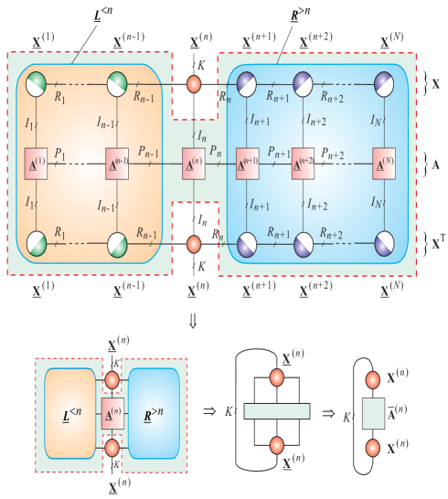
Refer to caption

Figure  27: Computation of K𝐾K eigenvectors corresponding to K𝐾K extreme eigenvalues in TT format for the symmetric matrix 𝐀I×I𝐀superscript𝐼𝐼{\bf A}\in\mathbb{R}^{I\times I} and the orthogonal matrix 𝐗I×K𝐗superscript𝐼𝐾{\bf X}\in\mathbb{R}^{I\times K} given in the distributed block tensor train formats. The extreme eigenvalues are computed as 𝚲=𝐗(n)T𝐀¯(n)𝐗(n)𝚲superscript𝐗𝑛𝑇superscript¯𝐀𝑛superscript𝐗𝑛\mbox{\boldmath$\Lambda$}={\bf X}^{(n)\;T}\bar{\bf A}^{(n)}{\bf X}^{(n)}.

Assuming that frame matrices have orthogonal columns, we can convert the optimization problem (49) into a set of linked optimization problems:

min𝐗(n)tr(𝐗(n)T𝐀¯(n)𝐗(n)),s.t.𝐗(n)T𝐗(n)=𝐈Ksubscriptsuperscript𝐗𝑛trsuperscript𝐗𝑛𝑇superscript¯𝐀𝑛superscript𝐗𝑛s.t.superscript𝐗𝑛𝑇superscript𝐗𝑛subscript𝐈𝐾\displaystyle\min_{{\bf X}^{(n)}}\mathop{\rm tr}\nolimits({\bf X}^{(n)\,T}\bar{\bf A}^{(n)}{\bf X}^{(n)}),\quad\mbox{s.t.}\;\;{\bf X}^{(n)\;T}{\bf X}^{(n)}={\bf I}_{K} (53)

for n=1,2,,N𝑛12𝑁n=1,2,\ldots,N, where 𝐀¯(n)superscript¯𝐀𝑛\bar{\bf A}^{(n)} is computed iteratively by tensor network contraction shown in Fig. 27 (b). In other words, the above problem is solved iteratively via optimized iterative contraction of the tensor network. This means that an active block (core) is sequentially selected in an iterative manner for n=1,2,,N𝑛12𝑁n=1,2,\ldots,N by sweeping from left to right and back from right to left and so on until convergence [68, 69].

It should be noted that the global orthogonality constraint 𝐗T𝐗=𝐈Ksuperscript𝐗𝑇𝐗subscript𝐈𝐾{\bf X}^{T}{\bf X}={\bf I}_{K} is equivalent to the set of local orthogonality constraints (𝐗(n))T𝐗(n)=𝐈K,nsuperscriptsuperscript𝐗𝑛𝑇superscript𝐗𝑛subscript𝐈𝐾for-all𝑛({\bf X}^{(n)})^{T}{\bf X}^{(n)}={\bf I}_{K},\;\forall n, since due to left and right orthogonality of the cores, we can write:

𝐗T𝐗superscript𝐗𝑇𝐗\displaystyle{\bf X}^{T}{\bf X} =\displaystyle= 𝐗(n)T𝐗nT𝐗n𝐗(n)superscript𝐗𝑛𝑇subscriptsuperscript𝐗𝑇absent𝑛subscript𝐗absent𝑛superscript𝐗𝑛\displaystyle{\bf X}^{(n)\,T}{\bf X}^{T}_{\neq n}{\bf X}_{\neq n}{\bf X}^{(n)}
=\displaystyle= 𝐗(n)T𝐗(n),n.superscript𝐗𝑛𝑇superscript𝐗𝑛for-all𝑛\displaystyle{\bf X}^{(n)\,T}{\bf X}^{(n)},\;\;\forall n.

VIII-B Tensor Networks for Tracking a Few Extreme Singular Values and Vectors for SVD and Sparse PCA

(a)
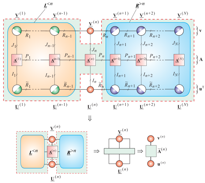
Refer to caption

(b)

Refer to caption
Figure  28: (a) Tensor network for computing the SVD singular eigenvectors corresponding to a largest singular value. (b) Tensor network for computing K𝐾K left- and right-eignevectors corresponding to the K𝐾K largest singular values via maximization of the trace tr(𝐔T𝐀𝐕)trsuperscript𝐔𝑇𝐀𝐕\mathop{\rm tr}\nolimits({\bf U}^{T}{\bf A}{\bf V}), subject to orthogonality constraints 𝐔T𝐔=𝐈ksuperscript𝐔𝑇𝐔subscript𝐈𝑘{\bf U}^{T}{\bf U}={\bf I}_{k} and 𝐕T𝐕=𝐈Ksuperscript𝐕𝑇𝐕subscript𝐈𝐾{\bf V}^{T}{\bf V}={\bf I}_{K} [73]. The singular values are computed as 𝚺=𝐔(n)T𝐀¯(n)𝐕(n)𝚺superscript𝐔𝑛𝑇superscript¯𝐀𝑛superscript𝐕𝑛\mbox{\boldmath$\Sigma$}={\bf U}^{(n)\;T}\bar{\bf A}^{(n)}{\bf V}^{(n)}.

The computation of the largest singular value and the corresponding left- and right eigenvector can be performed via the following optimization problem

max𝐮,𝐯{𝐮T𝐀𝐯},s.t.𝐮22=1,𝐯22=1,formulae-sequencesubscript𝐮𝐯superscript𝐮𝑇𝐀𝐯s.t.superscriptsubscriptnorm𝐮221superscriptsubscriptnorm𝐯221\displaystyle\max_{{\bf u},{\bf v}}\{{\bf u}^{T}{\bf A}{\bf v}\},\;\;\mbox{s.t.}\;\;||{\bf u}||_{2}^{2}=1,\;||{\bf v}||_{2}^{2}=1, (55)

where 𝐀I×J𝐀superscript𝐼𝐽{\bf A}\in\mathbb{R}^{I\times J} is arbitrary data matrix that admits low-rank TT decomposition. Using TT decomposition of vectors 𝐮I𝐮superscript𝐼{\bf u}\in\mathbb{R}^{I}, 𝐯J𝐯superscript𝐽{\bf v}\in\mathbb{R}^{J} and the data matrix 𝐀𝐀{\bf A} and assuming that cores 𝐔¯(n)superscript¯𝐔𝑛\underline{{\bf U}}^{(n)} and 𝐕¯(n)superscript¯𝐕𝑛\underline{{\bf V}}^{(n)} are kept left- and right- orthogonal, the optimization problem (55) can be converted into a set of usually much smaller scale optimization problems as follows (see Fig. 28 (a)):

max𝐮(n),𝐯(n){(𝐮(n))T𝐀¯(n)𝐯(n)},subscriptsuperscript𝐮𝑛superscript𝐯𝑛superscriptsuperscript𝐮𝑛𝑇superscript¯𝐀𝑛superscript𝐯𝑛\displaystyle\max_{{\bf u}^{(n)},{\bf v}^{(n)}}\{({\bf u}^{(n)})^{T}\bar{\bf A}^{(n)}{\bf v}^{(n)}\}, (56)
s.t.𝐮(n)22=1,𝐯(n)22=1,n,formulae-sequences.t.subscriptsuperscriptnormsuperscript𝐮𝑛221subscriptsuperscriptnormsuperscript𝐯𝑛221for-all𝑛\displaystyle\mbox{s.t.}\quad||{\bf u}^{(n)}||^{2}_{2}=1,\;\;||{\bf v}^{(n)}||^{2}_{2}=1,\;\forall n,

where 𝐮(n)=vec(𝐔¯(n))R~n1InR~nsuperscript𝐮𝑛𝑣𝑒𝑐superscript¯𝐔𝑛superscriptsubscript~𝑅𝑛1subscript𝐼𝑛subscript~𝑅𝑛{\bf u}^{(n)}=vec(\underline{{\bf U}}^{(n)})\in\mathbb{R}^{\widetilde{R}_{n-1}I_{n}\widetilde{R}_{n}} and 𝐯(n)=vec(𝐕¯(n))Rn1JnRnsuperscript𝐯𝑛𝑣𝑒𝑐superscript¯𝐕𝑛superscriptsubscript𝑅𝑛1subscript𝐽𝑛subscript𝑅𝑛{\bf v}^{(n)}=vec(\underline{{\bf V}}^{(n)})\in\mathbb{R}^{R_{n-1}J_{n}R_{n}} and

𝐀¯(n)=(𝐔n)T𝐀𝐕nR~n1InR~n×Rn1JnRnsuperscript¯𝐀𝑛superscriptsubscript𝐔absent𝑛𝑇subscript𝐀𝐕absent𝑛superscriptsubscript~𝑅𝑛1subscript𝐼𝑛subscript~𝑅𝑛subscript𝑅𝑛1subscript𝐽𝑛subscript𝑅𝑛\displaystyle\bar{\bf A}^{(n)}=({\bf U}_{\neq n})^{T}{\bf A}{\bf V}_{\neq n}\in\mathbb{R}^{\widetilde{R}_{n-1}I_{n}\widetilde{R}_{n}\times R_{n-1}J_{n}R_{n}} (57)

for n=1,2,,N𝑛12𝑁n=1,2,\ldots,N.

Note that taking into account that the frame matrices 𝐔nI1I2IN×R~n1InR~nsubscript𝐔absent𝑛superscriptsubscript𝐼1subscript𝐼2subscript𝐼𝑁subscript~𝑅𝑛1subscript𝐼𝑛subscript~𝑅𝑛{\bf U}_{\neq n}\in\mathbb{R}^{I_{1}I_{2}\cdots I_{N}\times\widetilde{R}_{n-1}I_{n}\widetilde{R}_{n}} and 𝐕nJ1J2JN×Rn1InRnsubscript𝐕absent𝑛superscriptsubscript𝐽1subscript𝐽2subscript𝐽𝑁subscript𝑅𝑛1subscript𝐼𝑛subscript𝑅𝑛{\bf V}_{\neq n}\in\mathbb{R}^{J_{1}J_{2}\cdots J_{N}\times R_{n-1}I_{n}R_{n}} are orthogonal and

𝐮=𝐔n𝐮(n),𝐯=𝐕n𝐯(n),n,formulae-sequence𝐮subscript𝐔absent𝑛superscript𝐮𝑛𝐯subscript𝐕absent𝑛superscript𝐯𝑛for-all𝑛\displaystyle{\bf u}={\bf U}_{\neq n}{\bf u}^{(n)},\;\;{\bf v}={\bf V}_{\neq n}{\bf v}^{(n)},\;\;\;\;\forall n, (58)

we can easily check that 𝐮2=𝐮(n)2subscriptnorm𝐮2subscriptnormsuperscript𝐮𝑛2||{\bf u}||_{2}=||{\bf u}^{(n)}||_{2} and 𝐯2=𝐯(n)2,nsubscriptnorm𝐯2subscriptnormsuperscript𝐯𝑛2for-all𝑛||{\bf v}||_{2}=||{\bf v}^{(n)}||_{2},\;\;\forall n.

An alternative approach to compute SVD for several maximal singular values and the corresponding left- and right- orthogonal eigenvectors, is to convert the SVD to the problem of symmetric EVD by applying the following basic relationships. It is evident, that from the SVD of the matrix 𝐀=𝐔𝚺𝐕TI×J𝐀𝐔𝚺superscript𝐕𝑇superscript𝐼𝐽{\bf A}={\bf U}\,\mbox{\boldmath$\Sigma$}\,{\bf V}^{T}\in\mathbb{R}^{I\times J}, where 𝚺1=diag{σ1,,σR}subscript𝚺1diagsubscript𝜎1subscript𝜎𝑅\mbox{\boldmath$\Sigma$}_{1}=\mathop{\rm diag}\nolimits\{\sigma_{1},\ldots,\sigma_{R}\}, we have

𝐀𝐀Tsuperscript𝐀𝐀𝑇\displaystyle{\bf A}{\bf A}^{T} =\displaystyle= 𝐔𝚺12𝐔T,𝐔subscriptsuperscript𝚺21superscript𝐔𝑇\displaystyle{\bf U}\mbox{\boldmath$\Sigma$}^{2}_{1}{\bf U}^{T}, (59)
𝐀T𝐀superscript𝐀𝑇𝐀\displaystyle{\bf A}^{T}{\bf A} =\displaystyle= 𝐕𝚺22𝐕T,𝐕subscriptsuperscript𝚺22superscript𝐕𝑇\displaystyle{\bf V}\,\mbox{\boldmath$\Sigma$}^{2}_{2}\,{\bf V}^{T}, (60)

where 𝚺1=diag{σ1,,σI}subscript𝚺1diagsubscript𝜎1subscript𝜎𝐼\mbox{\boldmath$\Sigma$}_{1}=\mathop{\rm diag}\nolimits\{\sigma_{1},\ldots,\sigma_{I}\} and 𝚺2=diag{σ1,,σI}subscript𝚺2diagsubscript𝜎1subscript𝜎𝐼\mbox{\boldmath$\Sigma$}_{2}=\mathop{\rm diag}\nolimits\{\sigma_{1},\ldots,\sigma_{I}\}. This means that the singular values of 𝐀I×J𝐀superscript𝐼𝐽{\bf A}\in\mathbb{R}^{I\times J} are the positive square roots of the eigenvalues of 𝐀T𝐀superscript𝐀𝑇𝐀{\bf A}^{T}{\bf A} and the eigenvectors 𝐔𝐔{\bf U} of 𝐀𝐀Tsuperscript𝐀𝐀𝑇{\bf A}{\bf A}^{T} are the left singular vectors of 𝐀𝐀{\bf A}. Note that if R<I𝑅𝐼R<I, the matrix 𝐀𝐀Tsuperscript𝐀𝐀𝑇{\bf A}{\bf A}^{T} will contain at least IR𝐼𝑅I-R additional eigenvalues that are not included as singular values of 𝐀𝐀{\bf A}.

Hence, in order to compute approximately K𝐾K smallest singular values and the corresponding right-eigenvectors, we can employ formally the following optimization problem:

min𝐕I×Ktr(𝐕T𝐀T𝐀𝐕),subscript𝐕superscript𝐼𝐾trsuperscript𝐕𝑇superscript𝐀𝑇𝐀𝐕\displaystyle\min_{{\bf V}\in\mathbb{R}^{I\times K}}\mathop{\rm tr}\nolimits({\bf V}^{T}{\bf A}^{T}{\bf A}{\bf V}), (61)
s.t.𝐕T𝐕=𝐈K.s.t.superscript𝐕𝑇𝐕subscript𝐈𝐾\displaystyle\mbox{s.t.}\quad{\bf V}^{T}\ {\bf V}={\bf I}_{K}.

The SVD problem for large–scale structured matrices that admit low-rank TT approximations can be solved iteratively in TT formats by the following set of smaller optimization (symmetric EVD) problems:

max𝐕(n)tr((𝐕(n))T[𝐕nT𝐀T𝐀𝐕n]𝐕(n)),subscriptsuperscript𝐕𝑛trsuperscriptsuperscript𝐕𝑛𝑇delimited-[]superscriptsubscript𝐕absent𝑛𝑇superscript𝐀𝑇subscript𝐀𝐕absent𝑛superscript𝐕𝑛\displaystyle\max_{{\bf V}^{(n)}}\mathop{\rm tr}\nolimits(({\bf V}^{(n)})^{T}[{\bf V}_{\neq n}^{T}{\bf A}^{T}{\bf A}{\bf V}_{\neq n}]{\bf V}^{(n)}), (62)
s.t.(𝐕(n))T𝐕(n)=𝐈K,n=1,2,,N,formulae-sequences.t.superscriptsuperscript𝐕𝑛𝑇superscript𝐕𝑛subscript𝐈𝐾𝑛12𝑁\displaystyle\mbox{s.t.}\quad({\bf V}^{(n)})^{T}{\bf V}^{(n)}={\bf I}_{K},\;\;n=1,2,\ldots,N,

where 𝐕(n)Rn1JnRn×Ksuperscript𝐕𝑛superscriptsubscript𝑅𝑛1subscript𝐽𝑛subscript𝑅𝑛𝐾{\bf V}^{(n)}\in\mathbb{R}^{R_{n-1}J_{n}R_{n}\times K} and

𝐀¯(n)=𝐕nT𝐀T𝐀𝐕nRn1InRn×Rn1InRnsuperscript¯𝐀𝑛superscriptsubscript𝐕absent𝑛𝑇superscript𝐀𝑇subscript𝐀𝐕absent𝑛superscriptsubscript𝑅𝑛1subscript𝐼𝑛subscript𝑅𝑛subscript𝑅𝑛1subscript𝐼𝑛subscript𝑅𝑛\displaystyle\bar{\bf A}^{(n)}={\bf V}_{\neq n}^{T}{\bf A}^{T}{\bf A}{\bf V}_{\neq n}\in\mathbb{R}^{R_{n-1}I_{n}R_{n}\times R_{n-1}I_{n}R_{n}} (63)

for n=1,2,,N𝑛12𝑁n=1,2,\ldots,N are computed sequentially via tensor network contractions as illustrated in Fig. 29.

(a)
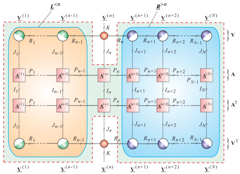
Refer to caption
(b)

Refer to caption
Figure  29: Computation of K𝐾K right eigenvectors corresponding to K𝐾K smallest singular values of the SVD in TT formats.

The challenge is how to extend and/or modify the above described approaches to the following large-scale optimization problems for structured matrices, if we need impose additional constraints such as sparsity, nonnegativity, orthogonality or local smoothness:

  • Sparse Principal Component Analysis (SPCA) using the Penalized Matrix Decomposition (PMD) [74, 75]

    max𝐮,𝐯{𝐮T𝐀𝐯},s.t.𝐮221,𝐯221,formulae-sequencesubscript𝐮𝐯superscript𝐮𝑇𝐀𝐯s.t.superscriptsubscriptnorm𝐮221superscriptsubscriptnorm𝐯221\displaystyle\max_{{\bf u},{\bf v}}\{{\bf u}^{T}{\bf A}{\bf v}\},\quad\mbox{s.t.}\quad||{\bf u}||_{2}^{2}\leq 1,\;\;||{\bf v}||_{2}^{2}\leq 1,
    P(𝐯)c1,𝑃𝐯subscript𝑐1\displaystyle P({\bf v})\leq c_{1}, (64)

    where the positive parameter c1subscript𝑐1c_{1} controls sparsity level and the convex penalty function P(𝐯)𝑃𝐯P({\bf v}) can take a variety of forms. Useful examples are [75]:

    P(𝐯)𝑃𝐯\displaystyle P({\bf v}) =\displaystyle= 𝐯1=i=1I|vi|(Lasso),subscriptnorm𝐯1superscriptsubscript𝑖1𝐼subscript𝑣𝑖(Lasso)\displaystyle||{\bf v}||_{1}=\sum_{i=1}^{I}|v_{i}|\quad\mbox{(Lasso)},
    P(𝐯)𝑃𝐯\displaystyle P({\bf v}) =\displaystyle= 𝐯0=i=1I|sign(vi)|,subscriptnorm𝐯0superscriptsubscript𝑖1𝐼signsubscript𝑣𝑖\displaystyle||{\bf v}||_{0}=\sum_{i=1}^{I}|\mathop{\rm sign}\nolimits(v_{i})|, (65)
    P(𝐯)𝑃𝐯\displaystyle P({\bf v}) =\displaystyle= i=1I|vi|+λi=2I|vivi1|.superscriptsubscript𝑖1𝐼subscript𝑣𝑖𝜆superscriptsubscript𝑖2𝐼subscript𝑣𝑖subscript𝑣𝑖1\displaystyle\sum_{i=1}^{I}|v_{i}|+\lambda\sum_{i=2}^{I}|v_{i}-v_{i-1}|.
  • SPCA via regularized SVD (sPCA-rSVD) [76], [77]

    max𝐮,𝐯{𝐮T𝐀𝐯αP(𝐯)}subscript𝐮𝐯superscript𝐮𝑇𝐀𝐯𝛼𝑃𝐯\displaystyle\max_{{\bf u},{\bf v}}\;\{{\bf u}^{T}{\bf A}{\bf v}-\alpha P({\bf v})\}
    s.t.𝐮221,𝐯221,formulae-sequences.t.superscriptsubscriptnorm𝐮221superscriptsubscriptnorm𝐯221\displaystyle\mbox{s.t.}\quad||{\bf u}||_{2}^{2}\leq 1,\;\;||{\bf v}||_{2}^{2}\leq 1, (66)
  • Two-way functional PCA/SVD [78]

    max𝐮,𝐯{𝐮T𝐀𝐯α2P1(𝐮)P2(𝐯)},subscript𝐮𝐯superscript𝐮𝑇𝐀𝐯𝛼2subscript𝑃1𝐮subscript𝑃2𝐯\displaystyle\max_{{\bf u},{\bf v}}\{{\bf u}^{T}{\bf A}{\bf v}-\frac{\alpha}{2}P_{1}({\bf u})P_{2}({\bf v})\},
    s.t.𝐮221,𝐯221.formulae-sequences.t.superscriptsubscriptnorm𝐮221superscriptsubscriptnorm𝐯221\displaystyle\mbox{s.t.}\quad||{\bf u}||_{2}^{2}\leq 1,\;\;||{\bf v}||_{2}^{2}\leq 1. (67)
  • Sparse SVD [79]

    max𝐮,𝐯{𝐮T𝐀𝐯12𝐮T𝐮𝐯T𝐯α12P1(𝐮)α22P2(𝐯)}.subscript𝐮𝐯superscript𝐮𝑇𝐀𝐯12superscript𝐮𝑇superscript𝐮𝐯𝑇𝐯subscript𝛼12subscript𝑃1𝐮subscript𝛼22subscript𝑃2𝐯\max_{{\bf u},{\bf v}}\{{\bf u}^{T}{\bf A}{\bf v}-\frac{1}{2}{\bf u}^{T}{\bf u}{\bf v}^{T}{\bf v}-\frac{\alpha_{1}}{2}P_{1}({\bf u})-\frac{\alpha_{2}}{2}P_{2}({\bf v})\}.\\ (68)
  • Generalized SPCA [80]

    max𝐮,𝐯{𝐮T𝐐𝐀𝐑𝐯α12P1(𝐮)α22P2(𝐯)},subscript𝐮𝐯superscript𝐮𝑇𝐐𝐀𝐑𝐯subscript𝛼12subscript𝑃1𝐮subscript𝛼22subscript𝑃2𝐯\displaystyle\max_{{\bf u},{\bf v}}\{{\bf u}^{T}{\bf Q}{\bf A}{\bf R}{\bf v}-\frac{\alpha_{1}}{2}P_{1}({\bf u})-\frac{\alpha_{2}}{2}P_{2}({\bf v})\},
    s.t.𝐮T𝐐𝐮1,𝐯T𝐑𝐯1,formulae-sequences.t.superscript𝐮𝑇𝐐𝐮1superscript𝐯𝑇𝐑𝐯1\displaystyle\mbox{s.t.}\quad{\bf u}^{T}{\bf Q}{\bf u}\leq 1,\;\;{\bf v}^{T}{\bf R}{\bf v}\leq 1, (69)

    where 𝐐T×T𝐐superscript𝑇𝑇{\bf Q}\in\mathbb{R}^{T\times T} and 𝐑I×I𝐑superscript𝐼𝐼{\bf R}\in\mathbb{R}^{I\times I} are symmetric positive-definite matrices.

  • Generalized nonnegative SPCA [81]

    max𝐮,𝐯{𝐮T𝐀𝐑𝐯α𝐯1},subscript𝐮𝐯superscript𝐮𝑇𝐀𝐑𝐯𝛼subscriptnorm𝐯1\displaystyle\max_{{\bf u},{\bf v}}\{{\bf u}^{T}{\bf A}{\bf R}{\bf v}-\alpha||{\bf v}||_{1}\},
    s.t.𝐮T𝐮1,𝐯T𝐑𝐯1,𝐯0.formulae-sequences.t.superscript𝐮𝑇𝐮1formulae-sequencesuperscript𝐯𝑇𝐑𝐯1𝐯0\displaystyle\mbox{s.t.}\quad{\bf u}^{T}{\bf u}\leq 1,\;\;{\bf v}^{T}{\bf R}{\bf v}\leq 1,\;\;{\bf v}\geq 0. (70)
TABLE IV: Cost functions and constraints used in classical feature extraction (dimension reduction) methods that can be formulated as generalized eigenvalue problem (71). The objective is to find an (orthogonal) matrix 𝐕𝐕{\bf V}, assuming that data matrices 𝐗𝐗{\bf X}, 𝐖,𝐃,𝐇𝐖𝐃𝐇{\bf W},{\bf D},{\bf H} are known. The symmetric matrix 𝐀𝐀{\bf A} can take different forms: 𝐀=𝐈1N𝟏𝟏T,𝐀=𝐃𝐖,𝐀=(𝐈𝐖T)(𝐈𝐖),𝐀=𝐈𝐇,formulae-sequence𝐀𝐈1𝑁superscript11𝑇formulae-sequence𝐀𝐃𝐖formulae-sequence𝐀𝐈superscript𝐖𝑇𝐈𝐖𝐀𝐈𝐇{\bf A}={\bf I}-\frac{1}{N}{\bf 11}^{T},\;{\bf A}={\bf D}-{\bf W},\;{\bf A}=({\bf I}-{\bf W}^{T})({\bf I}-{\bf W}),\;{\bf A}={\bf I}-{\bf H}, depending on method (for more detail see [82]).

Method Cost Function (min) Constraints Principal Component Analysis/ /Multi-Dimensional Scaling (PCA/MDS) tr[𝐕T𝐗(𝐈1N𝟏𝟏T)𝐗T𝐕]trdelimited-[]superscript𝐕𝑇𝐗𝐈1𝑁superscript11𝑇superscript𝐗𝑇𝐕\mathop{\rm tr}\nolimits[-{\bf V}^{T}{\bf X}({\bf I}-\frac{1}{N}{\bf 11}^{T}){\bf X}^{T}{\bf V}] 𝐕T𝐕=𝐈superscript𝐕𝑇𝐕𝐈{\bf V}^{T}{\bf V}={\bf I} Locally Preserving Projection (LPP) tr[𝐕T𝐗(𝐃𝐖)𝐗T𝐕]trdelimited-[]superscript𝐕𝑇𝐗𝐃𝐖superscript𝐗𝑇𝐕\mathop{\rm tr}\nolimits[{\bf V}^{T}{\bf X}({\bf D}-{\bf W}){\bf X}^{T}{\bf V}] 𝐕T𝐗𝐃𝐗T𝐕=𝐈superscript𝐕𝑇superscript𝐗𝐃𝐗𝑇𝐕𝐈{\bf V}^{T}{\bf XDX}^{T}{\bf V}={\bf I} Orthogonal LPP (OLPP) tr[𝐕T𝐗(𝐃𝐖)𝐗T𝐕]trdelimited-[]superscript𝐕𝑇𝐗𝐃𝐖superscript𝐗𝑇𝐕\mathop{\rm tr}\nolimits[{\bf V}^{T}{\bf X}({\bf{D-W}}){\bf X}^{T}{\bf V}] 𝐕T𝐕=𝐈superscript𝐕𝑇𝐕𝐈{\bf V}^{T}{\bf V}={\bf I} Neighborhood Preserving Projection (NPP) tr[𝐕T𝐗(𝐈𝐖T)(𝐈𝐖)𝐗T𝐕]trdelimited-[]superscript𝐕𝑇𝐗𝐈superscript𝐖𝑇𝐈𝐖superscript𝐗𝑇𝐕\mathop{\rm tr}\nolimits[{\bf V}^{T}{\bf X}({\bf I}-{\bf W}^{T})({\bf I}-{\bf W}){\bf X}^{T}{\bf V}] 𝐕T𝐗𝐗T𝐕=𝐈superscript𝐕𝑇superscript𝐗𝐗𝑇𝐕𝐈{\bf V}^{T}{\bf XX}^{T}{\bf V}={\bf I} Orthogonal NPP (ONPP) tr[𝐕T𝐗(𝐈𝐖T)(𝐈𝐖)𝐗T𝐕]trdelimited-[]superscript𝐕𝑇𝐗𝐈superscript𝐖𝑇𝐈𝐖superscript𝐗𝑇𝐕\mathop{\rm tr}\nolimits[{\bf V}^{T}{\bf X}({\bf I}-{\bf W}^{T})({\bf I}-{\bf W}){\bf X}^{T}{\bf V}] 𝐕T𝐕=𝐈superscript𝐕𝑇𝐕𝐈{\bf V}^{T}{\bf V}={\bf I} Linear Discriminant Analysis (LDA) tr[𝐕T𝐗(𝐈𝐇)𝐗T𝐕]trdelimited-[]superscript𝐕𝑇𝐗𝐈𝐇superscript𝐗𝑇𝐕\mathop{\rm tr}\nolimits[{\bf V}^{T}{\bf X}({\bf I}-{\bf H}){\bf X}^{T}{\bf V}] 𝐕T𝐗𝐗T𝐕=𝐈superscript𝐕𝑇superscript𝐗𝐗𝑇𝐕𝐈{\bf V}^{T}{\bf XX}^{T}{\bf V}={\bf I} Spectral Clustering (Ratio Cut) tr[𝐕T(𝐃𝐖)𝐕]trdelimited-[]superscript𝐕𝑇𝐃𝐖𝐕\mathop{\rm tr}\nolimits[{\bf V}^{T}({\bf D}-{\bf W}){\bf V}] 𝐕T𝐕=𝐈superscript𝐕𝑇𝐕𝐈{\bf V}^{T}{\bf V}={\bf I} Spectral Clustering (Normalized Cut) tr[𝐕T(𝐃𝐖)𝐕]trdelimited-[]superscript𝐕𝑇𝐃𝐖𝐕\mathop{\rm tr}\nolimits[{\bf V}^{T}({\bf D}-{\bf W}){\bf V}] 𝐕T𝐃𝐕=𝐈superscript𝐕𝑇𝐃𝐕𝐈{\bf V}^{T}{\bf DV}={\bf I}

Refer to caption
Figure  30: Tensor network for computation of K𝐾K eigenvectors corresponding to the K𝐾K extreme eigenvalues in TT formats for the generalized eigenvalue problem (71).

VIII-C Generalized Eigenvalue Problems in TT formats

In many practical applications, especially in dimension reduction and classification problems (e.g., in PCA/MDS, LPP, ONPP, LDA – see Table IV for more detail), we need to minimize the following trace optimization problem formulated as a generalized eigenvalue problem (GEVD) [82]:

min𝐕I×Ktr(𝐕T𝐗𝐀𝐗T𝐕),s.t.𝐕T𝐁𝐕=𝐈K,subscript𝐕superscript𝐼𝐾trsuperscript𝐕𝑇superscript𝐗𝐀𝐗𝑇𝐕s.t.superscript𝐕𝑇𝐁𝐕subscript𝐈𝐾\displaystyle\min_{{\bf V}\in\mathbb{R}^{I\times K}}\mathop{\rm tr}\nolimits({\bf V}^{T}{\bf X}{\bf A}{\bf X}^{T}{\bf V}),\quad\mbox{s.t.}\quad{\bf V}^{T}{\bf B}{\bf V}={\bf I}_{K}, (71)

where it is assumed that the structured data matrices: 𝐗I×J𝐗superscript𝐼𝐽{\bf X}\in\mathbb{R}^{I\times J}, symmetric matrix 𝐀J×J𝐀superscript𝐽𝐽{\bf A}\in\mathbb{R}^{J\times J}, and symmetric positive-definite matrix 𝐁I×I𝐁superscript𝐼𝐼{\bf B}\in\mathbb{R}^{I\times I} are known.

The problem is equivalent to the unconstrained optimization problem

min𝐕I×K{tr(𝐕T𝐗𝐀𝐗T𝐕)+α||𝐕T𝐁𝐕𝐈K||F2.\displaystyle\min_{{\bf V}\in\mathbb{R}^{I\times K}}\{\mathop{\rm tr}\nolimits({\bf V}^{T}{\bf X}{\bf A}{\bf X}^{T}{\bf V})+\alpha\;||{\bf V}^{T}{\bf B}{\bf V}-{\bf I}_{K}||^{2}_{F}. (72)

Note that by changing of the variable 𝐖=𝐁1/2𝐕𝐖superscript𝐁12𝐕{\bf W}={\bf B}^{1/2}{\bf V} the GEVD can be converted to the standard symmetric EVD problem

min𝐖I×Ktr(𝐖T𝐁1/2𝐗𝐀𝐗T𝐁1/2𝐖),s.t.𝐖T𝐖=𝐈K.subscript𝐖superscript𝐼𝐾trsuperscript𝐖𝑇superscript𝐁12superscript𝐗𝐀𝐗𝑇superscript𝐁12𝐖s.t.superscript𝐖𝑇𝐖subscript𝐈𝐾\displaystyle\min_{{\bf W}\in\mathbb{R}^{I\times K}}\mathop{\rm tr}\nolimits({\bf W}^{T}{\bf B}^{-1/2}{\bf X}{\bf A}{\bf X}^{T}{\bf B}^{-1/2}{\bf W}),\;\;\mbox{s.t.}\;\;{\bf W}^{T}{\bf W}={\bf I}_{K}.

The objective is to estimate the matrix 𝐕I×K𝐕superscript𝐼𝐾{\bf V}\in\mathbb{R}^{I\times K} in a TT format, assuming that large-scale matrices 𝐗𝐗{\bf X} and 𝐀𝐀{\bf A} (𝐖,𝐃,𝐇){\bf W},{\bf D},{\bf H}) are known and admit low-rank TT approximations. The problem for structured matrices that admit low-rank TT approximations can be solved iteratively:

min𝐕(n)tr((𝐕(n))T[𝐕nT𝐗𝐀𝐗T𝐕n]𝐕(n)),subscriptsuperscript𝐕𝑛trsuperscriptsuperscript𝐕𝑛𝑇delimited-[]superscriptsubscript𝐕absent𝑛𝑇superscript𝐗𝐀𝐗𝑇subscript𝐕absent𝑛superscript𝐕𝑛\displaystyle\min_{{\bf V}^{(n)}}\mathop{\rm tr}\nolimits(({\bf V}^{(n)})^{T}\;[{\bf V}_{\neq n}^{T}{\bf X}{\bf A}{\bf X}^{T}{\bf V}_{\neq n}]\;{\bf V}^{(n)}), (73)
s.t.(𝐕(n))T[𝐕nT𝐁𝐕n]𝐕(n)=𝐈K,s.t.superscriptsuperscript𝐕𝑛𝑇delimited-[]superscriptsubscript𝐕absent𝑛𝑇subscript𝐁𝐕absent𝑛superscript𝐕𝑛subscript𝐈𝐾\displaystyle\mbox{s.t.}\quad({\bf V}^{(n)})^{T}\;[{\bf V}_{\neq n}^{T}{\bf B}{\bf V}_{\neq n}]\;{\bf V}^{(n)}={\bf I}_{K},

where the relatively low-dimension matrices:

𝐀¯(n)=[𝐕nT𝐗𝐀𝐗T𝐕n]Rn1InRn×Rn1InRnsuperscript¯𝐀𝑛delimited-[]superscriptsubscript𝐕absent𝑛𝑇superscript𝐗𝐀𝐗𝑇subscript𝐕absent𝑛superscriptsubscript𝑅𝑛1subscript𝐼𝑛subscript𝑅𝑛subscript𝑅𝑛1subscript𝐼𝑛subscript𝑅𝑛\displaystyle\bar{\bf A}^{(n)}=[{\bf V}_{\neq n}^{T}{\bf X}{\bf A}{\bf X}^{T}{\bf V}_{\neq n}]\in\mathbb{R}^{R_{n-1}I_{n}R_{n}\times R_{n-1}I_{n}R_{n}} (74)

and

𝐁¯(n)=[𝐕nT𝐁𝐕n]Rn1InRn×Rn1InRnsuperscript¯𝐁𝑛delimited-[]superscriptsubscript𝐕absent𝑛𝑇subscript𝐁𝐕absent𝑛superscriptsubscript𝑅𝑛1subscript𝐼𝑛subscript𝑅𝑛subscript𝑅𝑛1subscript𝐼𝑛subscript𝑅𝑛\displaystyle\bar{\bf B}^{(n)}=[{\bf V}_{\neq n}^{T}{\bf B}{\bf V}_{\neq n}]\in\mathbb{R}^{R_{n-1}I_{n}R_{n}\times R_{n-1}I_{n}R_{n}} (75)

can be computed sequentially for n=1,2,,N𝑛12𝑁n=1,2,\ldots,N via tensor network contractions shown in Fig. 30.

VIII-D Canonical Correlation Analysis in TT Format

The Canonical Correlation Analysis (CCA), introduced by Hotelling, can be considered as a generalization of PCA and it is a classical method for determining the relationship between two sets of variables. Given two zero-mean (i.e., centered) data sets 𝐗I×J𝐗superscript𝐼𝐽{\bf X}\in\mathbb{R}^{I\times J} and 𝐘L×J𝐘superscript𝐿𝐽{\bf Y}\in\mathbb{R}^{L\times J} on the same set of J𝐽J observations, CCA seeks linear combinations of the variables in 𝐗𝐗{\bf X} and the variables in 𝐘𝐘{\bf Y} that are maximally mutually correlated with each other. Formally, the classical CCA computes two projection vectors 𝐰x=𝐰x(1)Isubscript𝐰𝑥subscriptsuperscript𝐰1𝑥superscript𝐼{\bf w}_{x}={\bf w}^{(1)}_{x}\in\mathbb{R}^{I} and 𝐰y=𝐰y(1)Lsubscript𝐰𝑦subscriptsuperscript𝐰1𝑦superscript𝐿{\bf w}_{y}={\bf w}^{(1)}_{y}\in\mathbb{R}^{L} such that the correlation coefficient

ρ=𝐰xT𝐗𝐘T𝐰y(𝐰xT𝐗𝐗T𝐰x)(𝐰yT𝐘𝐘T𝐰y)𝜌subscriptsuperscript𝐰𝑇𝑥superscript𝐗𝐘𝑇subscript𝐰𝑦subscriptsuperscript𝐰𝑇𝑥superscript𝐗𝐗𝑇subscript𝐰𝑥subscriptsuperscript𝐰𝑇𝑦superscript𝐘𝐘𝑇subscript𝐰𝑦\displaystyle\rho=\frac{{\bf w}^{T}_{x}{\bf X}{\bf Y}^{T}{\bf w}_{y}}{\sqrt{({\bf w}^{T}_{x}{\bf X}{\bf X}^{T}{\bf w}_{x})({\bf w}^{T}_{y}{\bf Y}{\bf Y}^{T}{\bf w}_{y})}} (76)

is maximized.

In a similar way, we can formulate kernel CCA by replacing inner product matrices by kernel matrices:

ρ=max𝜶x,𝜶y𝜶xT𝐊x𝐊y𝜶y(𝜶xT𝐊x𝐊x𝜶x)(𝜶yT𝐊y𝐊y𝜶y),𝜌subscriptsubscript𝜶𝑥subscript𝜶𝑦subscriptsuperscript𝜶𝑇𝑥subscript𝐊𝑥subscript𝐊𝑦subscript𝜶𝑦subscriptsuperscript𝜶𝑇𝑥subscript𝐊𝑥subscript𝐊𝑥subscript𝜶𝑥subscriptsuperscript𝜶𝑇𝑦subscript𝐊𝑦subscript𝐊𝑦subscript𝜶𝑦\displaystyle\rho=\max_{\mbox{\boldmath$\alpha$}_{x},\mbox{\boldmath$\alpha$}_{y}}\frac{\mbox{\boldmath$\alpha$}^{T}_{x}{\bf K}_{x}{\bf K}_{y}\mbox{\boldmath$\alpha$}_{y}}{\sqrt{(\mbox{\boldmath$\alpha$}^{T}_{x}{\bf K}_{x}{\bf K}_{x}\mbox{\boldmath$\alpha$}_{x})(\mbox{\boldmath$\alpha$}^{T}_{y}{\bf K}_{y}{\bf K}_{y}\mbox{\boldmath$\alpha$}_{y})}}, (77)

where 𝐊xJ×Jsubscript𝐊𝑥superscript𝐽𝐽{\bf K}_{x}\in\mathbb{R}^{J\times J} and 𝐊yJ×Jsubscript𝐊𝑦superscript𝐽𝐽{\bf K}_{y}\in\mathbb{R}^{J\times J} are suitably designed kernel matrices. The above optimization problem can be reformulated as a generalized eigenvalue decomposition (GEVD).

Since ρ𝜌\rho is invariant to the scaling of the vectors 𝐰xsubscript𝐰𝑥{\bf w}_{x} and 𝐰ysubscript𝐰𝑦{\bf w}_{y}, the standard CCA can be equivalently formulated as the following constrained optimization problem:

max𝐰x,𝐰y{𝐰xT𝐗𝐘T𝐰y}subscriptsubscript𝐰𝑥subscript𝐰𝑦superscriptsubscript𝐰𝑥𝑇superscript𝐗𝐘𝑇subscript𝐰𝑦\displaystyle\max_{{\bf w}_{x},{\bf w}_{y}}\{{\bf w}_{x}^{T}{\bf X}{\bf Y}^{T}{\bf w}_{y}\} (78)
s.t.𝐰xT𝐗𝐗T𝐰x=𝐰yT𝐘T𝐘𝐰y=1.s.t.superscriptsubscript𝐰𝑥𝑇superscript𝐗𝐗𝑇subscript𝐰𝑥superscriptsubscript𝐰𝑦𝑇superscript𝐘𝑇subscript𝐘𝐰𝑦1\displaystyle\mbox{s.t.}\quad{\bf w}_{x}^{T}{\bf X}{\bf X}^{T}{\bf w}_{x}={\bf w}_{y}^{T}{\bf Y}^{T}{\bf Y}{\bf w}_{y}=1. (79)

We will refer to 𝐭1=𝐗T𝐰xsubscript𝐭1superscript𝐗𝑇subscript𝐰𝑥{\bf t}_{1}={\bf X}^{T}{\bf w}_{x} and 𝐮1=𝐘T𝐰ysubscript𝐮1superscript𝐘𝑇subscript𝐰𝑦{\bf u}_{1}={\bf Y}^{T}{\bf w}_{y} as the canonical variables.

Refer to caption
Figure  31: Tensor network for computation of multiple (sparse) CCA.

For sparse CCA, we usually assume that the columns of 𝐗𝐗{\bf X} and 𝐘𝐘{\bf Y} have been standardized to have zero mean and standard deviation one. The cross product matrices 𝐗𝐗Tsuperscript𝐗𝐗𝑇{\bf X}{\bf X}^{T} and 𝐘𝐘Tsuperscript𝐘𝐘𝑇{\bf Y}{\bf Y}^{T} are often approximated by identity matrices, and consequently the constraints 𝐰xT𝐗𝐗T𝐰x1superscriptsubscript𝐰𝑥𝑇superscript𝐗𝐗𝑇subscript𝐰𝑥1{\bf w}_{x}^{T}{\bf X}{\bf X}^{T}{\bf w}_{x}\leq 1 and 𝐰yT𝐘𝐘T𝐰y1superscriptsubscript𝐰𝑦𝑇superscript𝐘𝐘𝑇subscript𝐰𝑦1{\bf w}_{y}^{T}{\bf Y}{\bf Y}^{T}{\bf w}_{y}\leq 1 can be simplified as 𝐰x221superscriptsubscriptnormsubscript𝐰𝑥221||{\bf w}_{x}||_{2}^{2}\leq 1 and 𝐰y221superscriptsubscriptnormsubscript𝐰𝑦221||{\bf w}_{y}||_{2}^{2}\leq 1, respectively under some conditions [75]. Hence, in order to compute sparse CCA we must impose suitable sparsity constraints on the canonical vectors, for example, by applying the PMD approach [74, 75]:

max𝐰x,𝐰y{𝐰xT𝐗𝐘T𝐰y}subscriptsubscript𝐰𝑥subscript𝐰𝑦superscriptsubscript𝐰𝑥𝑇superscript𝐗𝐘𝑇subscript𝐰𝑦\displaystyle\max_{{\bf w}_{x},{\bf w}_{y}}\{{\bf w}_{x}^{T}{\bf X}{\bf Y}^{T}{\bf w}_{y}\} (80)
s.t.𝐰x221,𝐰y221,formulae-sequences.t.superscriptsubscriptnormsubscript𝐰𝑥221superscriptsubscriptnormsubscript𝐰𝑦221\displaystyle\mbox{s.t.}\quad||{\bf w}_{x}||_{2}^{2}\leq 1,\;\;||{\bf w}_{y}||_{2}^{2}\leq 1,
P1(𝐰x)c1,P2(𝐰y)c2,formulae-sequencesubscript𝑃1subscript𝐰𝑥subscript𝑐1subscript𝑃2subscript𝐰𝑦subscript𝑐2\displaystyle P_{1}({\bf w}_{x})\leq c_{1},\;\;P_{2}({\bf w}_{y})\leq c_{2},

where P1subscript𝑃1P_{1} and P2subscript𝑃2P_{2} are convex penalty functions and positive parameters c1,c2subscript𝑐1subscript𝑐2c_{1},c_{2} control sparsity level. Since P1subscript𝑃1P_{1} and P2subscript𝑃2P_{2} are generally chosen to yield sparse projection vectors 𝐰xsubscript𝐰𝑥{\bf w}_{x} and 𝐰ysubscript𝐰𝑦{\bf w}_{y}, we call this criterion the sparse CCA (see Eqs. (VIII-B)).

In order to compute multiple canonical vectors for the standard CCA, we can formulate the following optimization problem:

max𝐖x,𝐖ysubscriptsubscript𝐖𝑥subscript𝐖𝑦\displaystyle\max_{{\bf W}_{x},{\bf W}_{y}} {tr(𝐖xT𝐗𝐘T𝐖y)},𝑡𝑟subscriptsuperscript𝐖𝑇𝑥superscript𝐗𝐘𝑇subscript𝐖𝑦\displaystyle\{tr({\bf W}^{T}_{x}{\bf X}{\bf Y}^{T}{\bf W}_{y})\}, (81)
s.t. 𝐖xT𝐗𝐗T𝐖x=𝐈Ksubscriptsuperscript𝐖𝑇𝑥superscript𝐗𝐗𝑇subscript𝐖𝑥subscript𝐈𝐾\displaystyle{\bf W}^{T}_{x}{\bf X}{\bf X}^{T}{\bf W}_{x}={\bf I}_{K}
𝐖yT𝐘𝐘T𝐖y=𝐈K,subscriptsuperscript𝐖𝑇𝑦superscript𝐘𝐘𝑇subscript𝐖𝑦subscript𝐈𝐾\displaystyle{\bf W}^{T}_{y}{\bf Y}{\bf Y}^{T}{\bf W}_{y}={\bf I}_{K},

where 𝐖x=[𝐰x(1),𝐰x(2),,𝐰x(K)]I×Ksubscript𝐖𝑥superscriptsubscript𝐰𝑥1superscriptsubscript𝐰𝑥2superscriptsubscript𝐰𝑥𝐾superscript𝐼𝐾{\bf W}_{x}=[{\bf w}_{x}^{(1)},{\bf w}_{x}^{(2)},\ldots,{\bf w}_{x}^{(K)}]\in\mathbb{R}^{I\times K} and 𝐖y=[𝐰y(1),𝐰y(2),,𝐰y(K)]L×Ksubscript𝐖𝑦superscriptsubscript𝐰𝑦1superscriptsubscript𝐰𝑦2superscriptsubscript𝐰𝑦𝐾superscript𝐿𝐾{\bf W}_{y}=[{\bf w}_{y}^{(1)},{\bf w}_{y}^{(2)},\ldots,{\bf w}_{y}^{(K)}]\in\mathbb{R}^{L\times K}.

This optimization scheme in a TT format is illustrated in Fig. 31 and performs iteratively the following set of optimization problems:

max𝐖x(n),𝐖y(n)tr((𝐖x(n))T[𝐖x,nT𝐗𝐘T𝐖y,n]𝐖y(n)),subscriptsubscriptsuperscript𝐖𝑛𝑥subscriptsuperscript𝐖𝑛𝑦trsuperscriptsuperscriptsubscript𝐖𝑥𝑛𝑇delimited-[]subscriptsuperscript𝐖𝑇𝑥absent𝑛superscript𝐗𝐘𝑇subscript𝐖𝑦absent𝑛subscriptsuperscript𝐖𝑛𝑦\displaystyle\max_{{\bf W}^{(n)}_{x},{\bf W}^{(n)}_{y}}\mathop{\rm tr}\nolimits(({\bf W}_{x}^{(n)})^{T}\;[{\bf W}^{T}_{x,\;\neq n}{\bf X}{\bf Y}^{T}{\bf W}_{y,\;\neq n}]\;{\bf W}^{(n)}_{y}),
s.t.(𝐖x(n))T[𝐖x,nT𝐗𝐗T𝐖x,n]𝐖x(n)=𝐈Ks.t.superscriptsuperscriptsubscript𝐖𝑥𝑛𝑇delimited-[]subscriptsuperscript𝐖𝑇𝑥absent𝑛superscript𝐗𝐗𝑇subscript𝐖𝑥absent𝑛subscriptsuperscript𝐖𝑛𝑥subscript𝐈𝐾\displaystyle\mbox{s.t.}\;\;({\bf W}_{x}^{(n)})^{T}\;[{\bf W}^{T}_{x,\;\neq n}{\bf X}{\bf X}^{T}{\bf W}_{x,\;\neq n}]\;{\bf W}^{(n)}_{x}={\bf I}_{K}
(𝐖y(n))T[𝐖y,nT𝐘𝐘T𝐖y,n]𝐖y(n)=𝐈K,superscriptsuperscriptsubscript𝐖𝑦𝑛𝑇delimited-[]subscriptsuperscript𝐖𝑇𝑦absent𝑛superscript𝐘𝐘𝑇subscript𝐖𝑦absent𝑛subscriptsuperscript𝐖𝑛𝑦subscript𝐈𝐾\displaystyle\qquad({\bf W}_{y}^{(n)})^{T}\;[{\bf W}^{T}_{y,\;\neq n}{\bf Y}{\bf Y}^{T}{\bf W}_{y,\;\neq n}]\;{\bf W}^{(n)}_{y}={\bf I}_{K},
n=1,2,,N.𝑛12𝑁\displaystyle\qquad n=1,2,\ldots,N. (82)

Note that for large-scale sparse CCA the cross product matrices 𝐗𝐗Tsuperscript𝐗𝐗𝑇{\bf X}{\bf X}^{T} and 𝐘𝐘Tsuperscript𝐘𝐘𝑇{\bf Y}{\bf Y}^{T} can be approximated by identity matrices, and consequently the above constraints can be simplified [74].

VIII-E Solving Large-Scale Systems of Linear Equations

Consider a huge system of linear algebraic equations in TT formats:

𝐀𝐱𝒚𝐀𝐱𝒚\displaystyle{\bf A}{\bf x}\cong\mbox{\boldmath$y$} (83)

or equivalently (if a matrix 𝐀𝐀{\bf A} is not symmetric positive-definite)

𝐀T𝐀𝐱𝐀T𝒚superscript𝐀𝑇𝐀𝐱superscript𝐀𝑇𝒚\displaystyle{\bf A}^{T}{\bf A}{\bf x}\cong{\bf A}^{T}\mbox{\boldmath$y$} (84)

where 𝐀I×J𝐀superscript𝐼𝐽{\bf A}\in\mathbb{R}^{I\times J}, (with IJ𝐼𝐽I\geq J), 𝒚I𝒚superscript𝐼\mbox{\boldmath$y$}\in\mathbb{R}^{I} and a matrix 𝐀T𝐀J×Jsuperscript𝐀𝑇𝐀superscript𝐽𝐽{\bf A}^{T}{\bf A}\in\mathbb{R}^{J\times J} is a symmetric positive-definite matrix which does not need to be explicitly computed (see Fig. 32). The objective is to find the vector 𝐱J𝐱superscript𝐽{\bf x}\in\mathbb{R}^{J} in a TT format.

To solve this problem in the Least Squares (LS) sense, we minimize the following cost function

J(𝐱)𝐽𝐱\displaystyle J({\bf x}) =\displaystyle= 𝐀𝐱𝒚22=(𝐀𝐱𝒚)T(𝐀𝐱𝒚)subscriptsuperscriptnorm𝐀𝐱𝒚22superscript𝐀𝐱𝒚𝑇𝐀𝐱𝒚\displaystyle||{\bf A}{\bf x}-\mbox{\boldmath$y$}||^{2}_{2}=({\bf A}{\bf x}-\mbox{\boldmath$y$})^{T}({\bf A}{\bf x}-\mbox{\boldmath$y$}) (85)
=\displaystyle= 𝐱T𝐀T𝐀𝐱2𝐱T𝐀T𝒚+𝒚T𝒚,superscript𝐱𝑇superscript𝐀𝑇𝐀𝐱2superscript𝐱𝑇superscript𝐀𝑇𝒚superscript𝒚𝑇𝒚\displaystyle{\bf x}^{T}{\bf A}^{T}{\bf A}{\bf x}-2{\bf x}^{T}{\bf A}^{T}\mbox{\boldmath$y$}+\mbox{\boldmath$y$}^{T}\mbox{\boldmath$y$},

which can be simplified to

J(𝐱)=𝐱T𝐀T𝐀𝐱2𝐱T𝐀T𝒚.𝐽𝐱superscript𝐱𝑇superscript𝐀𝑇𝐀𝐱2superscript𝐱𝑇superscript𝐀𝑇𝒚\displaystyle J({\bf x})={\bf x}^{T}{\bf A}^{T}{\bf A}{\bf x}-2{\bf x}^{T}{\bf A}^{T}\mbox{\boldmath$y$}. (86)

Using the TT representation of a matrix 𝐀𝐀{\bf A} and vectors 𝐱𝐱{\bf x} and 𝒚𝒚y [22, 21, 83], we have:

𝐀¯¯𝐀\displaystyle\underline{{\bf A}} =\displaystyle= 𝐀¯(1),𝐀¯(2),,𝐀¯(N)superscript¯𝐀1superscript¯𝐀2superscript¯𝐀𝑁\displaystyle\llbracket\underline{{\bf A}}^{(1)},\underline{{\bf A}}^{(2)},\ldots,\underline{{\bf A}}^{(N)}\rrbracket
𝐗¯¯𝐗\displaystyle\underline{{\bf X}} =\displaystyle= 𝐗¯(1),𝐗¯(2),,𝐗¯(N)superscript¯𝐗1superscript¯𝐗2superscript¯𝐗𝑁\displaystyle\llbracket\underline{{\bf X}}^{(1)},\underline{{\bf X}}^{(2)},\ldots,\underline{{\bf X}}^{(N)}\rrbracket (87)
𝐘𝐘\displaystyle{\bf Y} =\displaystyle= 𝐘(1),𝐘(2),,𝐘(N)superscript𝐘1superscript𝐘2superscript𝐘𝑁\displaystyle\llbracket{\bf Y}^{(1)},{\bf Y}^{(2)},\ldots,{\bf Y}^{(N)}\rrbracket

and upon applying the frame equation 𝐱=𝐗n𝐱(n)𝐱subscript𝐗absent𝑛superscript𝐱𝑛{\bf x}={\bf X}_{\neq n}{\bf x}^{(n)} with frame matrices

𝐗n=(𝐗(n)<n)T𝐈In(𝐗(1)>n)TJ1J2JN×Rn1JnRn,subscript𝐗absent𝑛tensor-productsuperscriptsubscriptsuperscript𝐗absent𝑛𝑛𝑇subscript𝐈subscript𝐼𝑛superscriptsubscriptsuperscript𝐗absent𝑛1𝑇superscriptsubscript𝐽1subscript𝐽2subscript𝐽𝑁subscript𝑅𝑛1subscript𝐽𝑛subscript𝑅𝑛\displaystyle{\bf X}_{\neq n}=({\bf X}^{<n}_{(n)})^{T}\otimes{\bf I}_{I_{n}}\otimes({\bf X}^{>n}_{(1)})^{T}\in\mathbb{R}^{J_{1}J_{2}\cdots J_{N}\times R_{n-1}J_{n}R_{n}},

the cost function can be written as

J(𝐱)=J(𝐗n𝐱(n))𝐽𝐱𝐽subscript𝐗absent𝑛superscript𝐱𝑛\displaystyle J({\bf x})=J({\bf X}_{\neq n}{\bf x}^{(n)}) =\displaystyle= (𝐱(n))T𝐗nT𝐀T𝐀𝐗n𝐱(n)superscriptsuperscript𝐱𝑛𝑇superscriptsubscript𝐗absent𝑛𝑇superscript𝐀𝑇subscript𝐀𝐗absent𝑛superscript𝐱𝑛\displaystyle({\bf x}^{(n)})^{T}{\bf X}_{\neq n}^{T}{\bf A}^{T}{\bf A}{\bf X}_{\neq n}{\bf x}^{(n)} (88)
2(𝐱(n))T𝐗nT𝐀T𝒚.2superscriptsuperscript𝐱𝑛𝑇superscriptsubscript𝐗absent𝑛𝑇superscript𝐀𝑇𝒚\displaystyle-2({\bf x}^{(n)})^{T}{\bf X}_{\neq n}^{T}{\bf A}^{T}\mbox{\boldmath$y$}.
Refer to caption
Refer to caption
Figure  32: Simplified tensor network scheme for solving systems of linear equations with a huge non-symmetric matrix 𝐀𝐀{\bf A}.

This converts the problem of solving a large-scale system of linear equations into to solving smaller system of algebraic equations iteratively

𝐀¯(n)𝐱(n)𝒚(n),n=1,2,,N,formulae-sequencesuperscript¯𝐀𝑛superscript𝐱𝑛superscript𝒚𝑛𝑛12𝑁\displaystyle\bar{\bf A}^{(n)}{\bf x}^{(n)}\cong\mbox{\boldmath$y$}^{(n)},\quad n=1,2,\ldots,N, (89)

where 𝐱(n)Rn1JnRnsuperscript𝐱𝑛superscriptsubscript𝑅𝑛1subscript𝐽𝑛subscript𝑅𝑛{\bf x}^{(n)}\in\mathbb{R}^{R_{n-1}J_{n}R_{n}} and

𝐀¯(n)superscript¯𝐀𝑛\displaystyle\bar{\bf A}^{(n)} =\displaystyle= 𝐗nT𝐀T𝐀𝐗nRn1JnRn×Rn1JnRn,superscriptsubscript𝐗absent𝑛𝑇superscript𝐀𝑇subscript𝐀𝐗absent𝑛superscriptsubscript𝑅𝑛1subscript𝐽𝑛subscript𝑅𝑛subscript𝑅𝑛1subscript𝐽𝑛subscript𝑅𝑛\displaystyle{\bf X}_{\neq n}^{T}{\bf A}^{T}{\bf A}{\bf X}_{\neq n}\in\mathbb{R}^{R_{n-1}J_{n}R_{n}\times R_{n-1}J_{n}R_{n}},
𝒚(n)superscript𝒚𝑛\displaystyle\mbox{\boldmath$y$}^{(n)} =\displaystyle= 𝐗nT𝐀T𝒚Rn1JnRn,superscriptsubscript𝐗absent𝑛𝑇superscript𝐀𝑇𝒚superscriptsubscript𝑅𝑛1subscript𝐽𝑛subscript𝑅𝑛\displaystyle{\bf X}_{\neq n}^{T}{\bf A}^{T}\mbox{\boldmath$y$}\in\mathbb{R}^{R_{n-1}J_{n}R_{n}}, (90)

under condition that cores are suitably left and right orthonormalized.

Of course, we cannot perform such matrix multiplications explicitly, but in TT formats, i.e., via iterative contraction of cores in the tensor network shown in Fig. 32.

The computations of a huge full vector 𝐱𝐱{\bf x} or 𝐀𝐱𝐀𝐱{\bf A}{\bf x} or a matrix 𝐀T𝐀superscript𝐀𝑇𝐀{\bf A}^{T}{\bf A} are not possible due to their extremely large sizes. Via tensorization, by representing them in TT/QTT formats, and iterative contractions of cores, we can avoid the curse of dimensionality.

An assumption that data admits low-rank TT/QTT approximation is a key factor in this approach. However, for data with weak structure the TT rank could be still large, which makes the calculation difficult or even impossible. The way how TT ranks are chosen and adapted during the algorithm is very important and various approaches to solve large structured linear systems have been proposed i [30, 22, 21, 84, 85, 86].

Remark. Some applications admit the use of even more complex TT networks with higher-order cores as illustrated in Fig. 33 (a) and (b), for which we can exploit biorthonormality constraints [87].

(a)
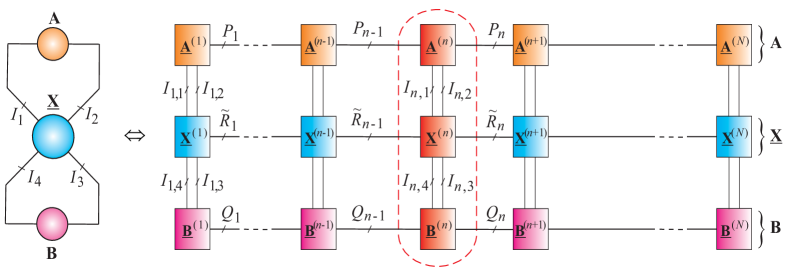
Refer to caption

(b)

Refer to caption
Figure  33: Representation of tensor traces in tensor train formats (see also Fig. 9). These models arise in some optimization problems, in which we need to maximize the tensor traces subject to additional constraints imposed on matrices.

VIII-F Software and Algorithms for Tensor Networks and Tensor Decompositions

Tensor decompositions and tensor networks algorithms require sophisticated software libraries, which are only now being developed.

For standard TDs (CPD, Tucker models) the Tensor Toolbox for MATLAB, originally developed by Kolda and Bader, provides several general-purpose commands and special facilities for handling sparse, dense, and structured standard TDs [88], while the N𝑁N-Way Toolbox for Matlab, by Andersson and Bro, has been developed mostly for Chemometrics [89]. Moreover, we recently developed the TDALAB (http://bsp.brain.riken.jp/TDALAB) and TENSORBOX (http://www.bsp.brain.riken.jp/~phan), which provides user-friendly interface and advanced algorithms for basic tensor decompositions: Tucker and CPD [90, 91].

The Tensorlab toolbox developed by Sorber, Van Barel and De Lathauwer builds upon a complex optimization framework and offers efficient numerical algorithms for computing the CPD, Block term Decomposition (BTD) or constrained Tucker decompositions. The toolbox includes a library of many constraints (e.g., nonnegativity, orthogonality) and offered the possibility to combine and jointly factorize dense, sparse and incomplete tensors [92].

Similar to the CPD and/or Tucker decompositions, the TT and HT decompositions are often based on generalized unfolding matrices 𝐗[n]subscript𝐗delimited-[]𝑛{\bf X}_{[n]}, and a good approximation in a decomposition for a given TT/HT-rank can be obtained from the SVDs of the unfolding matrices. In practice, we avoid the explicit construction of these matrices and the SVDs when truncating a tensor via the TT decomposition to lower TT-rank. Such truncation algorithms for TT are described in [40]. HT algorithms that avoid the explicit computation of these SVDs when truncating a tensor that is already in HT decomposition are discussed in [30, 35, 93].

In [94] Oseledets proposed for TT decomposition a new approximative formula in which a N𝑁Nth-order data tensor is interpolated using special form of Cross-Approximation, a modification of the CUR algorithm. The total number of entries and the complexity of the interpolation algorithm depend linearly on the order of data tensor N𝑁N, so the developed algorithm does not suffer from the curse of dimensionality. The TT-Cross-Approximation is analog to the SVD/HOSVD like algorithms for TT/MPS, but uses adaptive cross-approximation instead of the computationally more expensive SVD.

The TT Toolbox developed by Oseledets (http://spring.inm.ras.ru/osel/?page_id=24) focusses on TT and QTT structures, which deal with the curse of dimensionality [95]. The Hierarchical Tucker toolbox by Kressner and Tobler [35, 36] (http://www.sam.math.ethz.ch/NLAgroup/htucker_toolbox.html) and Tensor library by Handschuh, Waehnert and Espig, focus mostly on HT and TT tensor networks, while TensorCalculus by Espig at al. is a C++ library is for more general tensor networks [93].

In quantum physics and chemistry, a number of related software packages have been developed in the context of DMRG techniques for simulating quantum networks; see for example intelligent Tensor (iTensor) by Stoudenmire and White [96]. The iTensor Library is an open source C++ library for rapidly developing and applying tensor network algorithms. The iTensor is competitive with other available codes when performing basic DMRG calculations, but due to its flexibility it is especially well suited for developing next-generation tensor network algorithms such as PEPS.

Another promising software is the Universal Tensor Network Library (Uni10) developed in C++ by Yun-Da Hsieh and Ying-Jer Kao (from the National Taiwan University) which provides algorithms for performing contraction of a complicated tensor network with easy to use interface (http://uni10.org/about.html). The library is geared toward more complex tensor networks such as PEPS and MERA.

The problems related with optimization and improvements of several existing algorithms for TDs and TNs is an active area of research (see for example [97, 98, 92]).

IX Conclusions

Tensor networks, which can be considered as generalization and extension of tensor decompositions, are promising tools for analysis of big data, especially, for wide family of large-scale optimization problems due to their extremely good compression abilities and distributed processing of data (cloud computing). Moreover, TNs have the ability to address both the strong and the weak coupling between variables, and to deal with incomplete and noisy data. In fact, TDs have already found application in generalized multivariate regression, multi-way blind source separation, sparse representation and coding, feature extraction, classification, clustering and data assimilation [99, 100, 101, 102, 103, 104, 97].

From a more general perspective, the main concept for big data analytic is to apply a suitable tensorization of the data and to perform an approximate decomposition in TT/QTT formats. By constructing a suitable tensor network we can perform all matrix/vectors operations in tensor network formats. The use of the virtual tensorization or quantization (QTT) allows us to treat more efficiently very large-scale data [61, 62, 66].

In this paper, we have illuminated that tensor networks, especially tensor trains, are very promising tools for big data optimization problems, and have illustrated the natural and distributed representations offered by tensor networks for a selected class of optimization problems. This framework can be extended to a broader class of optimization problems, especially for extremely large-scale and untractable numerical problems.

In this approach a large-scale optimization problem is transformed into a set of small-scale linked optimization problems, each over a relative small group of unknown variables, which are grouped via TT decompositions and are represented by low-dimensional cores. In other words, by representing data in TT format we are able to turn a specific class of optimization problem into local tractable subproblems, which have the same structure or type as the original huge optimization problem. This allows us to apply any efficient numerical algorithm to local optimization problems.

The presented approach will work if only two assumptions are satisfied:

  1. 1.

    The structured data can be represented in TT formats that admit sufficiently good low-rank approximations.

  2. 2.

    Approximate solutions are acceptable [71].

Challenging problems related to low-rank tensor approximations remain that need to be addressed include:

  • Current implementations of tensor train decomposition and tensor contractions still require a number of tuning parameters, e.g., approximations accuracy, TT ranks estimation. Improved and semi-automatic TT approximation accuracy criteria, TT rank adaption and control and a priori errors bounds need to be developed. Particularly, the unpredictable accumulation of rounding error and TT-rank explosion problem should be better understood and solved [105].

  • Convergence analysis tools for TT algorithms should be developed and we need to better understand convergence properties of such algorithms.

  • As the complexity of big data increases, this requires more efficient iterative algorithms for their computing, extending beyond the ALS/MALS, DMRG, SVD/QR and CUR/Cross-Approximation class of algorithms.

  • Theoretic and methodological approaches are needed to determine what kind of constraints should be imposed on factor matrices/cores in order to extract desired hidden (latent) variables with meaningful physical interpretation.

  • Generalizations of Tensor Train models to more sophisticated tensor networks should be developed to fully integrate complex systems and optimization problems (e.g., a system simulating the biological molecule structure) [105].

  • Investigating the uniqueness of various TN models and optimality properties, or lack thereof, are needed and this may lead to faster and/or more reliable algorithms.

  • Special techniques are needed to save and process huge ultra large-scale tensors which occupy peta-bytes memory.

In summary, TNs is a fascinating and perspective area of research with many potential applications in optimization problems for massive big data sets.

References

  • [1] A. Cichocki, D. Mandic, C. Caiafa, A.-H. Phan, G. Zhou, Q. Zhao, and L. D. Lathauwer, “Multiway component analysis: Tensor decompositions for signal processing applications,” IEEE Signal Processing Magazine, 2014 (in print).
  • [2] A. Cichocki, “Era of big data processing: A new approach via tensor networks and tensor decompositions,” CoRR, vol. abs/1403.2048, 2014. [Online]. Available: http://arxiv.org/abs/1403.2048
  • [3] A. Cichocki, R. Zdunek, A.-H. Phan, and S. Amari, Nonnegative Matrix and Tensor Factorizations: Applications to Exploratory Multi-way Data Analysis and Blind Source Separation.   Chichester: Wiley, 2009.
  • [4] T. Kolda and B. Bader, “Tensor decompositions and applications,” SIAM Review, vol. 51, no. 3, pp. 455–500, September 2009.
  • [5] A. Cichocki, “Tensors decompositions: New concepts for brain data analysis?” Journal of Control, Measurement, and System Integration (SICE), vol. 47, no. 7, pp. 507–517, 2011.
  • [6] W. Hackbusch, Tensor Spaces and Numerical Tensor Calculus, ser. Springer series in computational mathematics.   Heidelberg: Springer, 2012, vol. 42.
  • [7] A. Smilde, R. Bro, and P. Geladi, Multi-way Analysis: Applications in the Chemical Sciences.   New York: John Wiley & Sons Ltd, 2004.
  • [8] P. Kroonenberg, Applied Multiway Data Analysis.   New York: John Wiley & Sons Ltd, 2008.
  • [9] D. Kressner, M. Steinlechner, and B. Vandereycken, “Low-rank tensor completion by Riemannian optimization,” BIT (in press), 2013.
  • [10] H. Wang, Q. Wu, L. Shi, Y. Yu, and N. Ahuja, “Out-of-core tensor approximation of multi-dimensional matrices of visual data,” ACM Trans. Graph., vol. 24, no. 3, pp. 527–535, 2005.
  • [11] S. K. Suter, M. Makhynia, and R. Pajarola, “Tamresh - tensor approximation multiresolution hierarchy for interactive volume visualization,” Comput. Graph. Forum, vol. 32, no. 3, pp. 151–160, 2013.
  • [12] A. H. Phan and A. Cichocki, “PARAFAC algorithms for large-scale problems,” Neurocomputing, vol. 74, no. 11, pp. 1970–1984, 2011.
  • [13] N. Lee and A. Cichocki, “Fundamental tensor operations for large-scale data analysis in tensor train formats,” ArXiv e-prints, May 2014. [Online]. Available: http://adsabs.harvard.edu/abs/2014arXiv1405.7786L
  • [14] R. Orus, “Exploring corner transfer matrices and corner tensors for the classical simulation of quantum lattice systems,” Phys.Rev., vol. B85, p. 205117, 2012.
  • [15] ——, “A Practical introduction to Tensor Networks: Matrix Product States and Projected Entangled Pair States,” The Journal of Chemical Physics, 2013.
  • [16] B. Khoromskij, “O(dlogN)𝑂𝑑𝑁O(d\log N)-quantics approximation of N𝑁N-d𝑑d tensors in high-dimensional numerical modeling,” Constructive Approximation, vol. 34, no. 2, pp. 257–280, 2011.
  • [17] P. Comon, X. Luciani, and A. L. F. de Almeida, “Tensor decompositions, Alternating Least Squares and other Tales,” Jour. Chemometrics, vol. 23, pp. 393–405, 2009.
  • [18] H. Lu, K. Plataniotis, and A. Venetsanopoulos, “A survey of multilinear subspace learning for tensor data,” Pattern Recognition, vol. 44, no. 7, pp. 1540–1551, 2011.
  • [19] M. Mørup, “Applications of tensor (multiway array) factorizations and decompositions in data mining,” Wiley Interdisc. Rew.: Data Mining and Knowledge Discovery, vol. 1, no. 1, pp. 24–40, 2011.
  • [20] N. Sidiropoulos, “Low-rank decomposition of multi-way arrays: A signal processing perspective,” in Proc. of the IIEEE SAM 2004, July 18-21, Sitges, Barcelona, 2004. [Online]. Available: http://www.sandia.gov/~tgkolda/tdw2004/Nikos04.pdf
  • [21] S. V. Dolgov and D. V. Savostyanov, “Alternating minimal energy methods for linear systems in higher dimensions. part ii: Faster algorithm and application to nonsymmetric systems,” arXiv preprint arXiv:1304.1222, 2013.
  • [22] ——, “Alternating minimal energy methods for linear systems in higher dimensions. part i: SPD systems,” arXiv preprint arXiv:1301.6068, 2013.
  • [23] A. H. Phan, A. Cichocki, P. Tichavsky, D. Mandic, and K. Matsuoka, “On revealing replicating structures in multiway data: A novel tensor decomposition approach,” in Proc. 10th International Conf. LVA/ICA, Tel Aviv, March 12-15,, 2012, pp. 297–305.
  • [24] R. N. C. Pfeifer, J. Haegeman, and F. Verstraete, “Faster identification of optimal contraction sequences for tensor networks,” ArXiv e-prints, Apr. 2013. [Online]. Available: http://adsabs.harvard.edu/abs/2013arXiv1304.6112P
  • [25] R. Pfeifer, G. Evenbly, S. Singh, and G. Vidal, “NCON: A tensor network contractor for MATLAB,” arXiv preprint arXiv:1402.0939, 2014.
  • [26] S. Rajbhandari, A. Nikam, P.-W. Lai, K. Stock, S. Krishnamoorthy, and P. Sadayappan, “Framework for distributed contractions of tensors with symmetry,” Preprint, Ohio State University, 2013.
  • [27] M. Lubasch, J. Cirac, and M.-C. Ba uls, “Unifying projected entangled pair state contractions,” New Journal of Physics, vol. 16, no. 3, p. 033014, 2014. [Online]. Available: http://stacks.iop.org/1367-2630/16/i=3/a=033014
  • [28] S. Sachdev, “Tensor networks¯a new tool for old problems,” Physics, vol. 2, p. 90, Oct 2009. [Online]. Available: http://link.aps.org/doi/10.1103/Physics.2.90
  • [29] M. Espig, W. Hackbusch, S. Handschuh, and R. Schneider, “Optimization problems in contracted tensor networks,” Comput. Visual. Sci., vol. 14, no. 6, pp. 271–285, 2011.
  • [30] L. Grasedyck, D. Kessner, and C. Tobler, “A literature survey of low-rank tensor approximation techniques,” CGAMM-Mitteilungen, vol. 36, pp. 53–78, 2013.
  • [31] L. Grasedyck and W. Hackbusch, “An introduction to hierarchical (h-) rank and tt-rank of tensors with examples,” Comput. Meth. in Appl. Math., vol. 11, no. 3, pp. 291–304, 2011.
  • [32] W. Hackbusch and S. Kühn, “A new scheme for the tensor representation,” Journal of Fourier Analysis and Applications, vol. 15, no. 5, pp. 706–722, 2009.
  • [33] L. Grasedyck, “Hierarchical Singular Value Decomposition of tensors,” SIAM J. Matrix Analysis Applications, vol. 31, no. 4, pp. 2029–2054, 2010.
  • [34] A. Uschmajew and B. Vandereycken, “The geometry of algorithms using hierarchical tensors,” Linear Algebra and its Applications, vol. 439, pp. 133—166, 2013.
  • [35] D. Kressner and C. Tobler, “htucker—A MATLAB toolbox for tensors in hierarchical Tucker format,” MATHICSE, EPF Lausanne (Preprint 2012), available at http://sma.epfl.ch/ anchpcommon/publications/htucker. pdf, 2012. [Online]. Available: http://anchp.epfl.ch/htucker
  • [36] ——, “Algorithm 941: htucker–A Matlab toolbox for tensors in Hierarchical Tucker format,” ACM Transactions on Mathematical Software (TOMS), vol. 40, no. 3, p. 22, 2014.
  • [37] C. Lubich, T. Rohwedder, R. Schneider, and B. Vandereycken, “Dynamical approximation of hierarchical Tucker and tensor-train tensors,” SIAM J. Matrix Anal. Appl., vol. 34, no. 2, pp. 470–494, 2013.
  • [38] I. Oseledets and E. E. Tyrtyshnikov, “Breaking the curse of dimensionality, or how to use SVD in many dimensions,” SIAM J. Scientific Computing, vol. 31, no. 5, pp. 3744–3759, 2009.
  • [39] G. Vidal, “Efficient classical simulation of slightly entangled quantum computations,” Physical Review Letters, vol. 91, no. 14, p. 147902, 2003.
  • [40] I. V. Oseledets, “Tensor-train decomposition,” SIAM J. Scientific Computing, vol. 33, no. 5, pp. 2295–2317, 2011.
  • [41] V. Kazeev, M. Khammash, M. Nip, and C. Schwab, “Direct solution of the Chemical Master Equation using Quantized Tensor Trains,” PLOS Computational Biology, March 2014.
  • [42] C. Lubich, I. Oseledets, and B. Vandereycken, “Time integration of tensor trains,” ArXiv e-prints, 2014.
  • [43] D. Bigoni, A. Engsig-Karup, and Y. Marzouk, “Spectral tensor-train decomposition,” arXiv preprint arXiv:1405.5713, 2014.
  • [44] I. Oseledets, E. Tyrtyshnikov, and N.Zamarashkin, “Tensor-train ranks for matrices and their inverses,” Comput. Meth. in Appl. Math., vol. 11, no. 3, pp. 394–403, 2011.
  • [45] D. Perez-Garcia, F. Verstraete, M. M. Wolf, and J. I. Cirac, “Matrix product state representations,” Quantum Info. Comput., vol. 7, no. 5, pp. 401–430, Jul. 2007. [Online]. Available: http://dl.acm.org/citation.cfm?id=2011832.2011833
  • [46] F. Verstraete, V. Murg, and J. Cirac, “Matrix product states, projected entangled pair states, and variational renormalization group methods for quantum spin systems,” Advances in Physics, vol. 57, no. 2, pp. 143–224, 2008.
  • [47] U. Schollwöck, “Matrix product state algorithms: DMRG, TEBD and relatives,” in Strongly Correlated Systems.   Springer, 2013, pp. 67–98.
  • [48] T. Huckle, K. Waldherr, and T. Schulte-Herbriggen, “Computations in quantum tensor networks,” Linear Algebra and its Applications, vol. 438, no. 2, pp. 750 – 781, 2013.
  • [49] U. Schollwöck, “The density-matrix renormalization group in the age of matrix product states,” Annals of Physics, vol. 326, no. 1, pp. 96–192, 2011.
  • [50] G. Evenbly and G. Vidal, “Algorithms for entanglement renormalization,” Physical Review B, vol. 79, no. 14, p. 144108, 2009.
  • [51] V. Giovannetti, S. Montangero, and R. Fazio, “Quantum multiscale entanglement renormalization ansatz channels,” Physical Review Letters, vol. 101, no. 18, p. 180503, 2008.
  • [52] J. Morton, “Tensor networks in algebraic geometry and statistics,” Lecture at Networking Tensor Networks, Centro de Ciencias de Benasque Pedro Pascual, Benasque, Spain, 2012.
  • [53] A. Critch and J. Morton, “Algebraic geometry of matrix product states,” ArXiv e-prints, Feb. 2014.
  • [54] A. Novikov and R. Rodomanov, “Putting MRFs on a tensor train,” in Proceedings of the International Conference on Machine Learning (ICML-14), 2014.
  • [55] A. Critch, “Algebraic Geometry of Hidden Markov and Related Models,” Ph.D. dissertation, University of California, Berkeley, 2013.
  • [56] S. Handschuh, “Changing the topology of tensor networks,” ArXiv e-prints, 2012.
  • [57] H. Zhao, Z. Xie, Q. Chen, Z. Wei, J. Cai, and T. Xiang, “Renormalization of tensor-network states,” Physical Review B, vol. 81, no. 17, p. 174411, 2010.
  • [58] R. Hübener, V. Nebendahl, and W. Dür, “Concatenated tensor network states,” New Journal of Physics, vol. 12, no. 2, p. 025004, 2010.
  • [59] I. Oseledets, “Approximation of 2d×2dsuperscript2𝑑superscript2𝑑2^{d}\times 2^{d} matrices using tensor decomposition,” SIAM J. Matrix Analysis Applications, vol. 31, no. 4, pp. 2130–2145, 2010.
  • [60] B. Khoromskij, “Tensors-structured numerical methods in scientific computing : Survey on recent advances,” Chemometrics and Intelligent Laboratory Systems, vol. 110, no. 1, pp. 1–19, 2011. [Online]. Available: http://www.mis.mpg.de/de/publications/preprints/2010/prepr2010-21.html
  • [61] S. Dolgov and B. Khoromskij, “Two-level QTT-Tucker format for optimized tensor calculus,” SIAM J. Matrix Analysis Applications, vol. 34, no. 2, pp. 593–623, 2013.
  • [62] V. Kazeev and B. Khoromskij, “Low-rank explicit QTT representation of the Laplace operator and its inverse,” SIAM J. Matrix Analysis Applications, vol. 33, no. 3, pp. 742–758, 2012.
  • [63] I. V. Oseledets and E. E. Tyrtyshnikov, “Algebraic wavelet transform via quantics tensor train decomposition,” SIAM J. Scientific Computing, vol. 33, no. 3, pp. 1315–1328, 2011.
  • [64] V. Kazeev, B. Khoromskij, and E. Tyrtyshnikov, “Multilevel Toeplitz matrices generated by tensor-structured vectors and convolution with logarithmic complexity,” SIAM J. Scientific Computing, vol. 35, no. 3, 2013.
  • [65] W. de Launey and J. Seberry, “The strong Kronecker product.” J. Comb. Theory, Ser. A, vol. 66, no. 2, pp. 192–213, 1994. [Online]. Available: http://dblp.uni-trier.de/db/journals/jct/jcta66.html#LauneyS94
  • [66] V. Kazeev, O. Reichmann, and C. Schwab, “Low-rank tensor structure of linear diffusion operators in the TT and QTT formats,” Linear Algebra and its Applications, vol. 438, no. 11, pp. 4204–4221, 2013.
  • [67] I. Pižorn and F. Verstraete, “Variational numerical renormalization group: Bridging the gap between NRG and density matrix renormalization group,” Phys. Rev. Lett., vol. 108, p. 067202, Feb 2012. [Online]. Available: http://link.aps.org/doi/10.1103/PhysRevLett.108.067202
  • [68] S. Dolgov, B. Khoromskij, I. Oseledets, and D. Savostyanov, “Computation of extreme eigenvalues in higher dimensions using block tensor train format,” Computer Physics Communications, vol. 185, no. 4, pp. 1207–1216, 2014.
  • [69] D. Kressner, M. Steinlechner, and A. Uschmajew, “Low-rank tensor methods with subspace correction for symmetric eigenvalue problems,” (in print), 2014. [Online]. Available: http://sma.epfl.ch/~uschmaje/paper/EVAMEN.pdf
  • [70] S. Holtz, T. Rohwedder, and R. Schneider, “The alternating linear scheme for tensor optimization in the tensor train format,” SIAM J. Scientific Computing, vol. 34, no. 2, 2012.
  • [71] D. Kressner and A. Uschmajew, “On low-rank approximability of solutions to high-dimensional operator equations and eigenvalue problems,” arXiv preprint arXiv:1406.7026, 2014.
  • [72] Z. Wen, C. Yang, X. Liu, and Y. Zhang, “Trace-penalty minimization for large-scale eigenspace computation,” DTIC Document, Tech. Rep., 2013.
  • [73] N. Lee and A. Cichocki, “Very large-scale singular value decomposition based on low-rank tensor train networks,” RIKEN BSI, Tech. Rep., 2014 (in preparation).
  • [74] D. Witten, R. Tibshirani, and T. Hastie, “A penalized matrix decomposition, with applications to sparse principal components and canonical correlation analysis,” Biostatistics, vol. 10, no. 3, pp. 515–534, 2009.
  • [75] D. Witten, “A penalized matrix decomposition, and its applications,” PhD Dissertation, Department of Statistics, Stanford University, 2010.
  • [76] H. Shen and J. Huang, “Sparse principal component analysis via regularized low rank matrix approximation,” Journal of Multivariable Analysis, vol. 99, no. 6, pp. 1015–1034, 2008. [Online]. Available: http://dx.doi.org/10.1016/j.jmva.2007.06.007
  • [77] M. Journee, Y. Nesterov, P. Richtarik, and R. Sepulchre, “Generalized power method for sparse principal component analysis,” Journal of Machine Learning Research, vol. 1, pp. 517–553, 2010.
  • [78] J. Huang, H. Shen, and A. Buja, “The analysis of two-way functional data using two-way regularized singular value decompositions,” Journal of the American Statistical Association, vol. 104, no. 488, pp. 1609–1620, 2009. [Online]. Available: http://EconPapers.repec.org/RePEc:bes:jnlasa:v:104:i:488:y:2009:p:1609-%1620
  • [79] M. Lee, H. Shen, J. Huang, and J. Marron, “Biclustering via sparse singular value decomposition.” Biometrics, vol. 66, no. 4, pp. 1087–1095, 2010. [Online]. Available: http://www.ncbi.nlm.nih.gov/pubmed/20163403
  • [80] G. Allen, “Regularized tensor factorizations and higher-order principal components analysis,” submitted, 2012. [Online]. Available: http://arxiv.org/pdf/1202.2476.pdf
  • [81] G. Allen and M. Maletic-Savatic, “Sparse non-negative generalized PCA with applications to metabolomics,” Bioinformatics, vol. 27 (21), pp. 3029–3035, 2011.
  • [82] E. Kokiopoulou, J. Chen, and Y. Saad, “Trace optimization and eigenproblems in dimension reduction methods,” Numerical Linear Algebra with Applications, vol. 18, no. 3, pp. 565–602, 2011.
  • [83] I. Oseledets and S. Dolgov, “Solution of linear systems and matrix inversion in the tt-format,” SIAM J. Scientific Computing, vol. 34, no. 5, 2012.
  • [84] S. Dolgov and I. Oseledets, “Solution of linear systems and matrix inversion in the tt-format,” SIAM J. Sci. Comput., vol. 34, no. 5, pp. A2718–A2739, 2011.
  • [85] S. Dolgov, “TT-GMRES: Solution to a linear system in the structured tensor format,” Russian Journal of Numerical Analysis and Mathematical Modelling, vol. 28, no. 2, pp. 149–172, 2013.
  • [86] I. Oseledets, “Dmrg approach to fast linear algebra in the tt-format,” Comput. Methods Appl. Math., vol. 11, no. 3, pp. 382–393, 2011.
  • [87] Y.-K. Huang, “Biorthonormal transfer-matrix renormalization-group method for non-Hermitian matrices,” Physical Review E, vol. 83, no. 3, p. 036702, 2011.
  • [88] B. Bader, T. G. Kolda et al., “MATLAB tensor toolbox version 2.5,” Available online, Feb. 2012. [Online]. Available: http://www.sandia.gov/~tgkolda/TensorToolbox/
  • [89] C. Andersson and R. Bro, “The N-way toolbox for MATLAB,” Chemometrics Intell. Lab. Systems, vol. 52, no. 1, pp. 1–4, 2000. [Online]. Available: http://www.models.life.ku.dk/source/nwaytoolbox/
  • [90] G. Zhou and A. Cichocki, “TDALAB: Tensor Decomposition Laboratory,” http://bsp.brain.riken.jp/TDALAB/, LABSP, Wako-shi, Japan, 2013. [Online]. Available: http://bsp.brain.riken.jp/TDALAB/
  • [91] A.-H. Phan, P. Tichavský, and A. Cichocki, “Tensorbox: a matlab package for tensor decomposition,” http://www.bsp.brain.riken.jp/ phan/tensorbox.php, Saitama, Japan, 2012.
  • [92] L. Sorber, M. Van Barel, and L. De Lathauwer, “Tensorlab v1.0,” Feb. 2013. [Online]. Available: http://esat.kuleuven.be/sista/tensorlab/
  • [93] M. Espig, M. Schuster, A. Killaitis, N. Waldren, P. Wähnert, S. Handschuh, and H. Auer, “TensorCalculus library,” 2012. [Online]. Available: http://gitorious.org/tensorcalculus
  • [94] I. Oseledets and E. Tyrtyshnikov, “TT-cross approximation for multidimensional arrays,” Linear Algebra and its Applications, vol. 432, no. 1, pp. 70–88, 2010.
  • [95] I. Oseledets, “TT-toolbox 2.2,” 2012. [Online]. Available: http://spring.inm.ras.ru/osel/?page_id=24
  • [96] E. Stoudenmire and S. White, “ITensor Library Release v0.2.5,” Perimeter Institute for Theoretical Physics, Tech. Rep., May 2014. [Online]. Available: {http://dx.doi.org/10.5281/zenodo.10068}
  • [97] G. Zhou, A. Cichocki, Q. Zhao, and S. Xie, “Efficient nonnegative Tucker decompositions: Algorithms and uniqueness,” CoRR, vol. abs/1404.4412, 2014. [Online]. Available: http://arxiv.org/abs/1404.4412
  • [98] A. H. Phan, P. Tichavsky, and A. Cichocki, “Low complexity Damped Gauss-Newton algorithms for CANDECOMP/PARAFAC,” SIAM Journal on Matrix Analysis and Applications (SIMAX) (in print), vol. arXiv/1205.2584, 2013. [Online]. Available: http://arxiv.org/pdf/1205.2584.pdf
  • [99] C. Caiafa and A. Cichocki, “Generalizing the column-row matrix decomposition to multi-way arrays,” Linear Algebra and its Applications, vol. 433, no. 3, pp. 557–573, 2010.
  • [100] ——, “Computing sparse representations of multidimensional signals using Kronecker bases,” Neural Computaion, vol. 25, no. 1, pp. 186–220, 2013.
  • [101] Q. Zhao, C. Caiafa, D. Mandic, Z. Chao, Y. Nagasaka, N. Fujii, L. Zhang, and A. Cichocki, “Higher-order partial least squares (HOPLS): A generalized multi-linear regression method, (in print),” IEEE Trans on Pattern Analysis and Machine Intelligence (PAMI), 2013 (in print).
  • [102] Q. Zhao, C. F. Caiafa, D. Mandic, L. Zhang, T. Ball, A. Schulze-bonhage, and A. S. Cichocki, “Multilinear subspace regression: An orthogonal tensor decomposition approach,” in Advances in Neural Information Processing Systems 24, J. Shawe-Taylor, R. Zemel, P. Bartlett, F. Pereira, and K. Weinberger, Eds., 2011, pp. 1269–1277.
  • [103] A. Phan and A. Cichocki, “Extended HALS algorithm for nonnegative Tucker decomposition and its applications for multi-way analysis and classification,” Neurocomputing, 2011.
  • [104] ——, “Tensor decompositions for feature extraction and classification of high dimensional datasets,” Nonlinear Theory and its Applications, IEICE, vol. 1, no. 1, pp. 37–68, 2010.
  • [105] D. Savostyanov, S. Dolgov, J. Werner, and I. Kuprov, “Exact NMR simulation of protein-size spin systems using tensor train formalism,” arXiv preprint arXiv:1402.4516, 2014.