Conformational properties of polymers in anisotropic environments
Abstract
We analyze the conformational properties of polymer macromolecules in solutions in presence of extended structural obstacles of (fractal) dimension causing the anisotropy of environment. Applying the pruned-enriched Rosenbluth method (PERM), we obtain numerical estimates for scaling exponents and universal shape parameters of polymers in such environments for a wide range in space dimension . An analytical description of the model is developed within the des Cloizeaux direct polymer renormalization scheme. Both numerical and analytical studies qualitatively confirm the existence of two characteristic length scales of polymer chain in directions parallel and perpendicular to the extended defects.
Key words: polymers, scaling, disorder, renormalization group, computer simulations
PACS: 36.20.-r, 89.75.Da, 64.60.ae, 07.05.Tp
Abstract
Проаналiзовано конформацiйнi властивостi полiмерних макромолекул у розчинах в присутностi протяжних структурних домiшок (фрактальної) вимiрностi , що спричиняють просторову анiзотропiю. Застосовуючи збiднено-збагачений алгоритм Розенблюта (PERM), отримано чисельнi оцiнки для скейлiнгових показникiв та унiверсальних характеристик форми полiмерiв у таких середовищах у широкому спектрi при вимiрностi простору . Аналiтичний опис моделi розвинено в рамках пiдходу прямого полiмерного перенормування де Клуазо. Як чисельнi, так i аналiтичнi дослiдження пiдтверджують iснування двох характеристичних масштабiв довжини полiмерного ланцюжка в паралельному та перпендикулярному напрямках до протяжних дефектiв.
Ключовi слова: полiмери, заморожений безлад, скейлiнг, ренормалiзацiйна група, чисельнi симуляцiї
1 Introduction
Many physical objects are characterized by anisotropy of structure: real magnetic crystals often contain extended defects in the form of linear dislocations, disclinations or planar regions of different phases [1, 2, 3, 4, 5]; in polymer systems, the understanding of the behavior of macromolecules in solutions having spatial anisotropy caused by the presence of fibrous obstacles is of great importance, e.g., in gels [6], intra- and extracellular environment [7, 8], or in the vicinity of planes (membranes) [9].
The analytical description of crystalline materials with extended defects attracts a lot of interest [1, 2, 3, 4, 5, 10, 11, 12, 13, 14]. In particular, Dorogovtsev [1] proposed the model of a -dimensional spin system with quenched nonmagnetic defects in the form of -dimensional objects, which are randomly distributed over the remaining dimensions. The anisotropy of the system brings about two different characteristic length scales (correlation lengths and ), reflecting the macroscopic properties of the system along the directions ‘‘parallel’’ to the -dimensional defect and along the ‘‘perpendicular’’ directions:
| (1.1) |
where is the reduced distance to the critical temperature , and are universal critical exponents.
A number of conformational properties of long flexible polymer chains in solutions can also be described within the critical exponent formalism: for example, the averaged mean-squared distance between two ends of a chain obeys the scaling law:
| (1.2) |
where is the number of monomers in the chain and is an universal quantity that does not depend on chemical properties of the macromolecule, but only on space dimension (e.g., the phenomenological Flory theory [15] gives ). Thus, for polymers in -dimensional space, this exponent takes on the maximal value of (completely stretched chain), in , one restores the exact value [16] and in the -dimensional case, the Flory theory nicely agrees, e.g., with the analytical result [17]. For space dimension , the polymer behaves as an idealized Gaussian chain with . The relation of the polymer size exponent (1.2) to the correlation length critical index of the -component spin vector model in the formal limit was provided by P.-G. de Gennes (the well-known de Gennes limit [15]).
Note that the Flory theory is applicable only in the case of polymers in a pure environment, but in reality most of the solutions contain impurities (obstacles), that interact with the macromolecules. These obstacles can be very small or penetrate through the whole space; randomly distributed or obeying some correlations on a mesoscopic scale [18, 19]. It was shown [20, 21, 22] that in the environment having a weak concentration of quenched point-like obstacles, the macromolecules behave like in pure solutions, namely the value of the critical exponent in (1.2) is the same as in the idealized case of a pure solvent. Only when the concentration of defects is close to the percolation threshold where an incipient percolation cluster of fractal structure emerges in the system, the scaling properties of polymers are modified in a non-trivial way [21, 22, 23, 24, 25, 26, 27, 20, 28, 29, 30, 31, 32, 33, 34, 35, 36, 37, 38, 39, 40]. It is appropriate to mention that according to a simple generalization of the Flory formula [21], there should be a different behavior for polymers on spaces with fractal dimension , e.g., on percolation clusters.
The conformational properties are also influenced in a non-trivial way when the position of one obstacle particle affects the other, i.e., there are correlations in the spatial distribution of impurities. In particular, these correlations often express themselves by a power law behavior [41] with , where is the distance between two obstacles. This type of disorder has a direct interpretation for integer values of , namely, the cases describe straight lines (planes) of impurities of random orientation, whereas non-integer values of are interpreted in terms of impurities organized in fractal structures. This type of disorder leads to a new universality class of polymers [42].
Herein above we were speaking about polymers in disordered but isotropic environment. It means that all the observable statistical properties of the molecules are the same when explored in different spatial directions. An interesting question concerns a quantitative change of these properties when there are some selected directions in the system: the case of spatial anisotropy. In this concern, a widely discussed model of directed self-avoiding walks (DSAW) [43] may describe the properties of macromolecules in an applied external field. This causes an elongation of the molecule along the field direction [44, 45] and leads to the existence of two characteristic length scales in parallel and perpendicular directions. The anisotropic properties of the environment can also be caused by the presence of extended obstacles correlated in -dimensions, similar to those discussed previously for the spin systems. These may be ordered colloid particles, gel fibers or biological species in a cell environment. In these systems we should also expect a different behavior along the chosen direction and perpendicular to it. Baumgartner and Muthukumar [46] discussed a model of polymer chains in an environment having impurities in the form of absorbing parallel cylinders. They predicted that the polymer chain is elongated in the direction parallel to the cylinders and, correspondingly, the parallel component of the end-to-end distance is governed by an exponent , whereas in normal direction there will be no dependence of the end-to-end distance component on the number of monomers at all (exponent ). This gives a reason to expect an anisotropic behavior for polymers in solution having impurities correlated in dimensions [47].
In the present paper, we study the conformational properties of polymers in the environment where an anisotropy is caused by the presence of -dimensional defects of parallel orientation, which are randomly distributed in the remaining dimensions, both using numerical simulations based on a discrete lattice model (Section II) and an analytical description within des Cloizeaux direct polymer renormalization scheme (Section III). We end up by giving conclusions and an outlook.
2 Numerical studies
2.1 The model
Our goal is to investigate the conformational properties of polymers in anisotropic environments in the presence of obstacles that are ordered in some subspace. For this purpose, we choose a lattice model of a long flexible polymer chain — the model of self-avoiding random walks (SAW), which is established to perfectly capture the universal properties of polymers in good solvent with the excluded volume effect. We deal with the cubic lattice since it is known that universal properties do not depend on the lattice type [51] and the cubic one is the most simple and easy to realize.
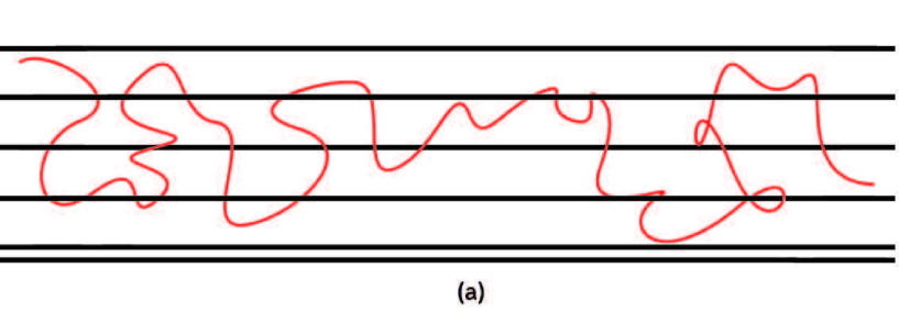
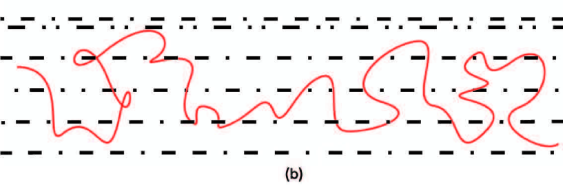
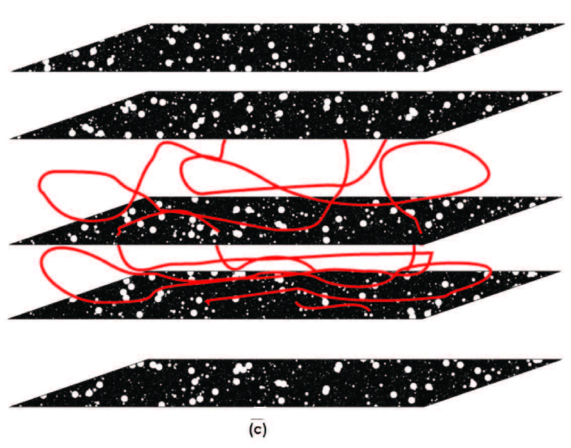
The simplest types of extended obstacles that can be chosen for our purposes are spacial objects in the form of lines () of parallel orientation (see figure 1 (a)), spreading throughout the lattice in some chosen direction, since they should obviously lead to a different behavior in directions parallel and perpendicular to them. The case of homogeneous planes is not of interest since they divide the space into small restricted regions, and thus the problem is reduced to that of polymers in confined geometries.
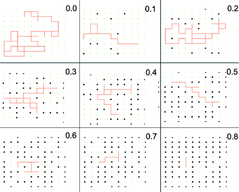
We start with an -plane of a lattice with concentration of randomly chosen sites containing point-like defects and then we build lines perpendicular to this plane in -direction through chosen sites. In figure 2 one can see a projection of the SAW trajectory on this plane for different concentrations of lines. As one can see at high concentrations of such obstacles, the SAW trajectory appears to collapse in small restricted regions. In this case, a long polymer chain will behave like a one-dimensional rod, extended in the direction parallel to the lines of defects. Thus, we expect a crossover to an extended regime for an increasing defect concentration.
We also consider more interesting situations, namely a set of partially penetrable lines (figure 1 (b)) and planes (figure 1 (c)). To this end, with some fixed probability , we randomly choose the sites on the constructed lines (planes) of defects and treat them as ‘‘open’’ (allowed for SAW trajectory). Note that one can, roughly speaking, treat these objects as fractals. For example, the fractal (cluster) dimension of such a line with concentration of the lacking sites can be estimated from the well-known relation between the linear size of an object and ‘‘the number of particles’’: (here, is the length of a line). Indeed, at , one has a Euclidian line (like in figure 1 (a)) and simply restores , whereas with increasing , the line can be treated as a set of disconnected sites (points) and the fractal dimension of this object gradually tends to 0.
2.2 The method
For our purposes we use the Pruned-Enriched Rosenbluth Method (PERM) [52]. It is based on the original Rosenbluth-Rosenbluth algorithm of growing chains with population control parameters [53]. On each step , the chain has a weight given by:
| (2.1) |
where is the number of possibilities to perform the next step, which varies from to due to the fact that the chain may not cross itself. This value is also reduced by the presence of impurities.
When the chain of total length is constructed, a new one is started from the same starting point, until the desired number of chain configurations are obtained. In this manner, all observables should be averaged over an ensemble of different chain configurations :
| (2.2) |
here, is the weight of the -th configuration of the -step trajectory.
It is also necessary to average over different configurations of disorder:
| (2.3) |
where is the number of replicas (the number of different realizations of the disorder). For our purposes, we consider about chains for each of the replicas.
Weight fluctuations are reduced by using population control (pruning and enrichment). It means that with probability of we reject the chains having low weight and enrich the statistics by replication increasing the number of high weighted configurations. To do this, we use lower and upper bound weights, that are updated at each step according to [54, 55, 56]: and , where is the number of chains of length created, and the parameter controls the pruning-enrichment statistics; it is chosen in such a way to allow one to receive in average chains of total length in each tour.
2.3 Results
We concentrate on the conformational properties of long flexible polymer chains, in particular, in the critical exponents governing the behavior of the effective linear size of the macromolecule with respect to the number of monomers (1.2). Let us note that in the anisotropic case we expect to have two different exponents rather than one:
| (2.4) |
so that . The parallel and perpendicular components are expected to behave in a different way [46].
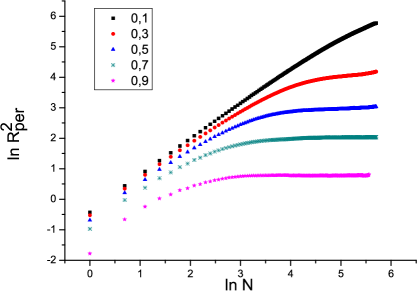
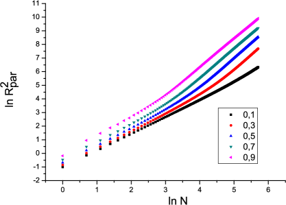
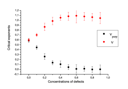
We start by considering the case of the anisotropy caused by the presence of obstacles in the form of impenetrable parallel lines [47]. In this case, we took chains up to monomers and find the components of the end-to-end distance vector, performing double averaging according to (2.3). The results are presented in figure 3. It is clearly observed that the behavior of the two components differ from each other: the parallel component grows with an increase of concentration of obstacles, whereas the perpendicular component collapses indicating the stretching of the polymer chain in longitudinal direction. As one can see, there is a crossover between the two types of behavior: one for short chains (less than monomers) and then the other one for long polymers. We expect this crossover to take place when the averaged end-to-end distance of the SAW trajectory is comparable to the distance between the lines of impurities. This is similar to the polymer behavior in a restricted space, for example a cylinder, when short chains (with end-to-end distance smaller than the radius of cylinder) behave like -dimensional, and long chains as -dimensional [15]. In our case, we observe a crossover to such a behavior when the concentration of lines that penetrate the system is close to a percolative concentration of point-like defects on a simple square lattice. At smaller concentrations, applying the least-square fitting of the data observed, we obtain the estimates for the two critical exponents and (see figure 4), which coincide at , where we restore the corresponding value of the SAW exponent on a pure lattice. As one can see, the exponent governing the scaling of a parallel component of the end-to-end distance is larger than the pure one and gradually reaches the maximal value of 1 with an increasing concentration of disorder, while is smaller and gradually tends to zero. It gives us the right to say that polymers in anisotropic space are more elongated than polymers in isotropic environments.
Let us check the fact of possible elongation by analyzing the shape properties. All information concerning the shape measure of a chain is given by the gyration tensor with its components defined by:
| (2.5) |
where are the components of the position vector of the -th monomer. Eigenvalues of this tensor provide a full information on the shape of the polymer. To receive these in simulations we need to solve a cubic equation for each of the chains. Thus, we are interested in calculating the rotationally invariant shape characteristics, such as asphericity and prolateness, defined in as combinations of gyration tensor components according to [48, 49, 50]:
| (2.6) |
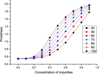
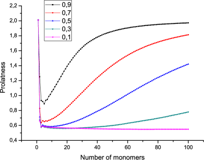
with ( being a unity matrix). Asphericity is normalized in such a way that it changes the value from for spherical configuration to for a completely stretched rod-like structure. Prolateness obeys the inequality: , it is negative for oblate configurations and positive for prolate ones; a value corresponds to a rod-like (completely prolate) state.
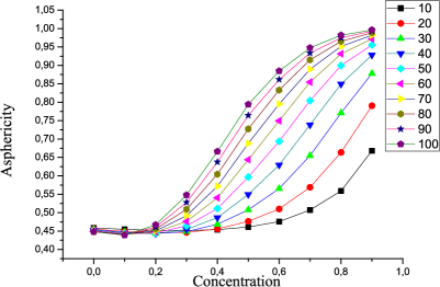
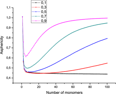
In figures 5 and 6 we present our data for and , averaged over realizations of disorder at various fixed concentrations of defects. At , in both cases we restore the corresponding values on a pure lattice. One can easily see in figures 5 (a) and 6 (a) that both quantities are growing with an increasing defect concentration and gradually reach the corresponding values of rod-like structures.
Next, we consider an interesting situation, where point-like defects in the lattice are aligned in some particular direction (say, ) forming partially penetrable lines (see figure 1 (b)). To investigate the influence of such a type of space anisotropy on the conformational properties of flexible polymer chains, we randomly choose some concentration of sites on lines of defects (constructed as described previously), and treat them as ‘‘open’’ (allowed to SAW trajectory). As a result, we obtain aligned fractal-like objects with dimension . In such problems, we have two parameters: the concentration of obstacles in the form of parallel lines, and the probability of a SAW trajectory to penetrate through this line.
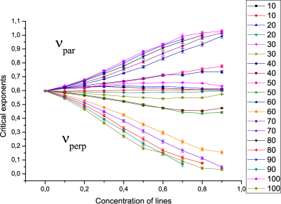
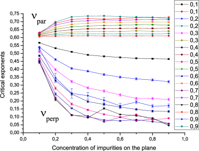
Performing simulations for chains up to steps and applying the least-square fits for the data obtained for parallel and perpendicular components of the end-to-end distances of polymer chains, we received the estimates for critical exponents and (see figure 7 (a)) as functions of these two parameters. Again, the exponent governing the scaling of a parallel component of the end-to-end distance is larger than the pure one and gradually reaches the maximal value of 1, while the other one is lower and gradually tends to zero. This tendency is kept even at a rather high probability of a growing trajectory to penetrate the line (up to the concentration of ‘‘open’’ sites close to a critical percolation concentration). When is close to 1, the spatial anisotropy disappears and both exponents gradually reach the corresponding value of the pure lattice case.
Finally, we consider another possible model of anisotropic environment caused by the presence of structural defects in the form of partially penetrable planes of parallel orientation (see figure 1 (c)). We start with homogeneous planes of concentration , randomly distributed in -direction, and again randomly choose some concentration of sites on these planes and treat them as ‘‘open’’(allowed to SAW trajectory). As a result, we obtain fractal-like objects having dimension . Performing simulations for chains up to steps and applying the least-square fits for data obtained for parallel and perpendicular components of the end-to-end distances of polymer chains, we receive estimates for the critical exponents and (see figure 7 (b)) as functions of these two parameters. The exponent governing the scaling of the parallel component of the end-to-end distance gradually changes from the value on three-dimensional pure lattice (at ) to that in two dimensions with a growing concentration of impurity planes. This can be treated as a crossover to a restricted geometry regime of polymers confined between two planes. The exponent gradually tends to zero.
3 Analytical approach
3.1 The model
We deal with flexible polymers in an environment with extended impurities correlated in -dimensions and randomly distributed in the remaining space. Let us start with a continuous x‘model, where a polymer chain is presented as a path of length (or surface) parameterized by , with [57]. An effective Hamiltonian of the system is given by:
| (3.1) |
Here, the first term describes the chain connectivity, the second term reflects the short-range repulsion between monomers due to the excluded volume effect with coupling constant , and the last term arises due to the interaction between the monomers of the polymer chain and the structural defects in the environment given by potential . We work in the formalism of partition functions:
where denotes integration over different paths.
Dealing with systems that display randomness of structure, one usually encounters two types of ensemble averaging, treated as annealed and quenched disorder [58, 59]. In general, the critical behavior of disordered systems with annealed and quenched averaging is quite different. However, for the polymer systems it has been shown [28, 60, 61, 62, 63], that the distinction between quenched and annealed averages for an infinitely long single polymer chain is negligible, and in performing analytical calculations for quenched polymer systems one may restrict the problem to the simpler case of annealed averaging. In this paper, we deal with annealed averaging over disorder because it is technically simpler. After averaging the partition sum over realizations of disorder and including only up to the second moment of cumulant expansion, we receive:
where gives the average concentration of impurities , and for the second moment we assume [46, 1]:
| (3.2) |
which reflects the fact that the impurities are correlated in dimensions and uncorrelated in the remaining space. Omitting the terms , which give a trivial constant shift, we obtain an averaged partition function with an effective Hamiltonian:
| (3.3) | |||||
Note that the last term in (3.3) describes an effective attractive interaction between monomers in the direction perpendicular to the extended obstacles governed by a coupling constant .
3.2 The method
Within the model, all the parameters depend on the polymer area and on dimensionless coupling constants (here is dimension of coupling constant ) in a way that when , one restores the case of idealized Gaussian chain without any interactions between monomers. To calculate the universal properties of the model we need to find such values of parameters that lead to physical values of the universal characteristics. For that reason, we use the direct renormalization technique proposed by des Cloiseaux [51].
Within this scheme, renormalized coupling constants are defined by:
| (3.4) |
where is the deviation from the upper space dimension for the coupling constant . is the swelling factor that governs the behavior of the end-to-end distance of the polymer in solution. It can be presented as a perturbation theory series over the coupling constants:
| (3.5) |
where the first term () corresponds to an ideal Gaussian chain and the others give corrections caused by interactions in the system. is the factor that depends only on the dimension of the corresponding coupling constant. This factor allows us to estimate the critical exponent using the relation:
The factor is connected with the partition function . Here, is the partition function of an idealized Gaussian chain, is the partition function of two interacting polymer chains.
Renormalized coupling constants given by the equation (3.4) tend to constant values or the so-called fixed points as the polymer area tends to infinity. The fixed points are defined as common zeros of the flow equations:
| (3.6) |
To find the fixed points of the model, one need to express in terms of and find the common zeros of (3.6) and then choose those that are stable and physical in the region of interest for the parameters .
3.3 Results
We start with the restricted partition function
| (3.7) |
where means averaging with the hamiltonian (3.3). We consider the evaluation of the expression (3.7) by performing the perturbation theory expansion in coupling constants , . The terms in this expansion can be presented diagrammatically as shown in figure 8. The first diagram describes the zeroth order approach corresponding to the idealized Gaussian chain without any interaction between the monomers. Solid line on the diagrams presents the polymer chain, the dashed line describes the excluded volume interaction between monomers governed by the coupling , and the wavy line presents the attractive interaction caused by the presence of the impurities governed by the coupling . Let us consider the expressions corresponding to the second and third diagram:
| (3.8) |
It is necessary to point out that in the expression for , the integration is performed only in subspace due to the fact that the interaction acts only in this subspace. Using the Poisson formula to integrate over the wave vector we receive:
| (3.9) |

Expanding the exponents over and then integrating over areas we finally receive:
| (3.10) |
where and are dimensionless coupling constants.
Collecting all contributions from the considered diagrams one receives an expression for the partition function of the model by keeping terms that do not depend on :
The expressions for the components of the end-to-end distance of the polymer chain can be estimated using the identities:
We distinguish between the components in subspaces and , corresponding to components of the end-to-end distance in directions parallel and perpendicular to extended defects:
| (3.11) | ||||
| (3.12) |
References (3.11) and (3.12) confirm the existence of two characteristic lengths for polymers in anisotropic environments. The presence of extended defects makes the polymer radius shrink in transverse direction due to the attractive interactions between monomers governed by the coupling , whereas in parallel direction, the increase of the effect of repulsive interactions (as consequence of the increase of monomer density) is responsible for the elongation of the polymer chains.
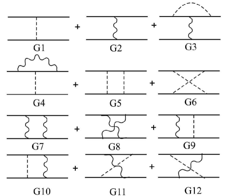
Calculating contributions to the partition function of two interacting polymer chains one may use a diagrammatic representation (see figure 9). Note that only those diagrams are taken into account which contain at least one interaction line. The first few diagrams, those with one interaction acting between two polymers (), can be gathered and presented as . Performing the dimensional analysis of the contributions, produced by different diagrams, we find two distinct classes of graphs. The first class of graphs produces terms which behave like , the sum of all such terms gives contributions into the function denoted by . The diagrams of the second class behave like and thus give contributions into the function . As a result, the ‘‘two polymer function’’ can be presented in the form: where and are given by the expressions:
| (3.13) | |||||
The swelling factor in our model reads:
| (3.14) |
The renormalized coupling constants can be presented in the form:
The corresponding flow equations read:
here, , . The coordinates of fixed points can be found as common zeros of functions ,:
| (3.15) | ||||
| (3.16) | ||||
| (3.17) | ||||
| (3.18) |
The first fixed point describes the case of an idealized Gaussian chain without any interactions between monomers. Expression (3.16) corresponds to the case of a polymer chain with short-range excluded volume interactions in a pure solvent. The fixed points (3.17) and (3.18) describe, correspondingly, the Gaussian chain and the chain with excluded volume effect in the anisotropic environment. However, since both of them are associated with attractive interactions between monomers due to the presence of defects, these fixed points appear to be unstable in the physical region of the parameters ( and ) and thus cannot provide estimates of scaling exponents. Note that a similar problem of the absence of stable and physically accessible fixed points also exists in the case of uncorrelated point-like impurities [24]. The latter was solved by absorbing the interaction with disorder into the excluded volume interaction due to a special symmetry [64]. However, this does not work in the present case of extended defects.
4 Conclusions
We analyzed the influence of anisotropy of the environment caused by the presence of impurities correlated in dimensions, on conformational size and shape characteristics of long flexible polymer chains. The integer values of have direct physical interpretation and describe extended defects, e.g., in the form of lines or planes of parallel orientation ( or , correspondingly). In this case, it is obvious that one should distinguish between two characteristic length scales, in directions parallel and perpendicular to such extended defects. Non-integer values of may correspond to complex defects of fractal nature.
Applying the numerical simulations based on the model of self-avoiding random walks on a regular cubic lattice, we considered three cases: impurities in the form of parallel lines (), fractal-like structures with (which can be treated as partially penetrable lines) and fractal-like structures with (partially penetrable planes). In the first case, we found that components of the effective linear size of polymer chain, that are either parallel or perpendicular to the lines of impurities, behave differently and their scaling is governed by two distinct scaling exponents and (see equation (2.4)). The exponent governing the scaling of a parallel component of the end-to-end distance gradually reaches the maximal value of 1 with increasing of concentration of defects, while gradually tends to zero. Analyzing the influence of disorder in the form of partially penetrable lines on scaling properties of polymers, we again found the existence of two distinct exponents and (see figure 7 (a)). This tendency (and thus the anisotropy) surprisingly persists even at high probability of the polymer chain to penetrate through such ‘‘line’’ (which corresponds to close to ). Considering structural defects in the form of partially penetrable planes of parallel orientation (see figure 1 (c)), we found that the exponent gradually changes from the value found earlier for the three-dimensional pure lattice to that in two dimensions with growing concentration of impurity planes. This can be treated as a crossover to a restricted geometry regime of the polymer confined between two homogeneous planes. The exponent gradually tends to zero.
Our analytical studies were performed within the frames of the direct polymer renormalization approach using the double , expansion. In particular, we found expressions for the components of the end-to-end distance of polymer chain (3.11), (3.12). The presence of extended defects makes the polymer radius shrink in transverse direction due to attractive interactions between monomers governed by the coupling , whereas in parallel direction the increase of the effect of repulsive interactions (as a consequence of the increase of monomer density) is responsible for the elongation of the polymer chain. We conclude that the presence of extended defects correlated in dimensions makes the polymer chain elongated in the direction parallel to these extended impurities, which confirms the existence of two characteristic lengths for polymers in anisotropic environments.
Acknowledgements
This work was supported in part by the FP7 EU IRSES projects N269139 ‘‘Dynamics and Cooperative Phenomena in Complex Physical and Biological Media’’ and N295302 ‘‘Statistical Physics in Diverse Realizations’’.
References
- [1] Dorogovtsev S.M., Fiz. Tverd. Tela (Leningrad), 1980, 22, 321.
- [2] Yamazaki Y., Holz A., Ochiai M., Fukuda Y., Physica A, 1988, 150, 576; doi:10.1016/0378-4371(88)90257-9.
- [3] Yamazaki Y., Holz A., Ochiai M., Fukuda Y., Phys. Rev. B, 1986, 33, 3460; doi:10.1103/PhysRevB.33.3460.
- [4] Yamazaki Y., Holz A., Ochiai M., Fukuda Y., Physica A, 1986, 136, 303; doi:10.1016/0378-4371(86)90255-4.
- [5] Yamazaki Y., Ochiai M., Holz A., Fukuda Y., Phys. Rev. B, 1986, 33, 3474; doi:10.1103/PhysRevB.33.3474.
-
[6]
Stylianopoulos T., Diop-Frimpong B., Munn L.L., Jain R.K.,
Biophys. J., 2010, 99, 3119;
doi:10.1016/j.bpj.2010.08.065. - [7] Xiao F., Nicholson C., Hrabe J., Hrabětova S., Biophys. J., 2008, 95, 1382; doi:10.1529/biophysj.107.124743.
- [8] Verkman A.S., Phys. Biol., 2013, 10, 045003; doi:10.1088/1478-3975/10/4/045003.
- [9] Cannell D.S. Rondelez F., Macromolecules, 1980, 13, 1599; doi:10.1021/ma60078a046.
- [10] Boyanovsky D., Cardy J.L., Phys. Rev. B, 1982, 33, 154; doi:10.1103/PhysRevB.26.154.
- [11] Lawrie I.D., Prudnikov V.V., J. Phys. C: Solid State Phys., 1984, 17, 1655; doi:10.1088/0022-3719/17/10/007.
- [12] Lee J.C., Gibbs R.L., Phys. Rev. B, 1992, 45, 2217; doi:10.1103/PhysRevB.45.2217.
- [13] De Cesare L., Phys. Rev. B, 1994, 49, 11742; doi:10.1103/PhysRevB.49.11742.
-
[14]
Korzhenevskii A.L., Herrmanns K., Schirmacher W.,
Phys. Rev. B, 1996, 53, 14834;
doi:10.1103/PhysRevB.53.14834. - [15] De Gennes P.G., Scaling Concepts in Polymer Physics, Cornell University Press, Ithaca, 1979.
- [16] Nienhuis B., Phys. Rev. Lett., 1982, 49, 1062; doi:10.1103/PhysRevLett.49.1062.
- [17] Guida R., Zinn-Justin J., J. Phys. A: Math. Gen., 1998, 31, 8104; doi:10.1088/0305-4470/31/40/006.
- [18] Sahimi M., Flow and Transport in Porous Media and Fractured Rock, VCH, Weinheim, 1995.
- [19] Dullen A.L., Porous Media: Fluid Transport and Pore Structure, Academic, New York, 1979.
- [20] Kim Y., J. Phys. A: Math. Gen., 1987, 20, 1293; doi:10.1088/0305-4470/20/5/039.
- [21] Kremer K., Z. Phys. B: Condens. Matter, 1981, 49, 149; doi:10.1007/BF01293328.
- [22] Lee S.B., Nakanishi H., Phys. Rev. Lett., 1988, 61, 2022; doi:10.1103/PhysRevLett.61.2022.
- [23] Lee S.B., Nakanishi H., Kim Y., Phys. Rev. B, 1989, 33, 9561; doi:10.1103/PhysRevB.39.9561.
- [24] Chakrabarti B.K., Kertesz K., Z. Phys. B: Condens. Matter, 1981, 44, 221; doi:10.1007/BF01297178.
- [25] Sahimi M., J. Phys. A: Math. Gen., 17, 1984, L379; doi:10.1088/0305-4470/17/7/002.
- [26] Lam P.M., Zhang Z.Q., Z. Phys. B: Condens. Matter, 1984, 56, 155; doi:10.1007/BF01469696.
- [27] Lyklema J.W., Kremer K., Z. Phys. B: Condens. Matter, 1984, 55, 41; doi:10.1007/BF01307499.
- [28] Cherayil B.J., J. Chem. Phys., 1990, 92, 6246; doi:10.1063/1.458349.
- [29] Roy A.K., Blumen A., J. Stat. Phys., 1990, 59, 1581; doi:10.1007/BF01334765.
- [30] Lam P.M., J. Phys. A: Math. Gen., 1990, 23, L831; doi:10.1088/0305-4470/23/16/010.
- [31] Kim Y., Phys. Rev. A, 1992, 45, 6103; doi:10.1103/PhysRevA.45.6103.
- [32] Nakanishi H., Lee S.B., J. Phys. A: Math. Gen., 1991, 24, 1355; doi:10.1088/0305-4470/24/6/026.
- [33] Vanderzande C., Komoda A., Phys. Rev. A, 1992, 45, R5335; doi:10.1103/PhysRevA.45.R5335.
-
[34]
Ordemann A., Porto M., Roman H.E., Havlin S., Bunde A.,
Phys. Rev. E, 2000, 61, 6858;
doi:10.1103/PhysRevE.61.6858. - [35] Janssen H.-K., Stenull O., Phys. Rev. E, 2007, 75, 020801R; doi:10.1103/PhysRevE.75.020801.
- [36] Grassberger P., J. Phys. A: Math. Gen., 1993, 26, 1023; doi:10.1088/0305-4470/26/5/022.
- [37] Lee S.B., J. Korean Phys. Soc., 1996, 29, 1.
- [38] Blavatska V., Janke W., Europhys. Lett., 2008, 82, 66006; doi:10.1209/0295-5075/82/66006.
- [39] Blavatska V., Janke W., Phys. Rev. Lett., 2008, 101, 125701; doi:10.1103/PhysRevLett.101.125701.
- [40] Blavatska V., Janke W., J. Phys. A: Math. Theor., 2009, 42, 015001; doi:10.1088/1751-8113/42/1/015001.
- [41] Weinrib A., Halperin B.I., Phys. Rev. B, 1983, 27, 413; doi:10.1103/PhysRevB.27.413.
- [42] Blavats’ka V., von Ferber C., Holovatch Yu., Phys. Rev. E, 2001, 64, 041102; doi:10.1103/PhysRevE.64.041102.
- [43] Vanderzande C., Lattice Models of Polymers, Cambridge University Press, Cambridge, 1998.
- [44] Bhattacharjee S.M., Physica A, 1992, 186, 183; doi:10.1016/0378-4371(92)90374-Y.
- [45] Baram A., Stern P.S., J. Phys. A: Math. Gen., 1985, 17, 1835; doi:10.1088/0305-4470/18/10/036.
- [46] Baumgartner A., Muthukumar M., In: Advances in Chemical Physics. Polymeric Systems, Vol. XCIV, Prigogine I., Rice S.A. (Eds.), John Wiley & Sons, New York, 1996, 625–709.
- [47] Blavatska V., Haydukivska K., Eur. Phys. J. – Spec. Top., 2013, 216, 191; doi:10.1140/epjst/e2013-01742-2.
- [48] Šolc K., Stockmayer W.H., J. Chem. Phys., 1971, 54, 2756; doi:10.1063/1.1675241.
- [49] Šolc K., J. Chem. Phys., 1971, 55, 335; doi:10.1063/1.1675527.
- [50] Aronovitz J.A., Nelson D.R., J. Phys., 1986, 47, 1445; doi:10.1051/jphys:019860047090144500.
- [51] Des Cloizeaux J., Jannink G., Polymers in Solutions: Their Modelling and Structure, Clarendon Press, Oxford, 1990.
- [52] Grassberger P., Phys. Rev. E, 1997, 56, 3682; doi:10.1103/PhysRevE.56.3682.
- [53] Rosenbluth M.N., Rosenbluth A.W., J. Chem. Phys., 1955, 23, 356; doi:10.1063/1.1741967.
- [54] Hsu H.P., Mehra V., Nadler W., Grassberger P., J. Chem. Phys., 2007, 118, 444; doi:10.1063/1.1522710.
- [55] Bachmann M., Janke W., Phys. Rev. Lett., 2003, 91, 208105; doi:10.1103/PhysRevLett.91.208105.
- [56] Bachmann M., Janke W., J. Chem. Phys., 2004, 120, 6779; doi:10.1063/1.1651055.
- [57] Edwards S.F., Proc. Phys. Soc. London, 1965, 85, 613; doi:10.1088/0370-1328/85/4/301.
- [58] Brout R., Phys. Rev., 1959, 115, 824; doi:10.1103/PhysRev.115.824.
- [59] Folk R., Holovatch Yu., Yavors’kii T., Phys.-Usp., 2003, 46, 169; doi:10.1070/PU2003v046n02ABEH001077.
- [60] Wu D., Hui K., Chandler D., J. Chem. Phys., 1991, 96, 835; doi:10.1063/1.462469.
- [61] Ippolito I., Bideau D., Hansen A., Phys. Rev. E, 1998, 57, 3656; doi:10.1103/PhysRevE.57.3656.
- [62] Patel D.M., Fredrickson G.H., Phys. Rev. E, 2003, 68, 051802; doi:10.1103/PhysRevE.68.051802.
- [63] Blavatska V., J. Phys.: Condens. Matter, 2013, 25, 505101; doi:10.1088/0953-8984/25/50/505101.
- [64] Kim Y., J. Phys. C: Solid State Phys., 1983, 16, 1345; doi:10.1088/0022-3719/16/8/005.
Ukrainian \adddialect\l@ukrainian0 \l@ukrainian Конформацiйнi властивостi полiмерiв в анiзотропних середовищах К. Гайдукiвська, В. Блавацька
Iнститут фiзики конденсованих систем НАН України, вул. I. Свєнцiцького, 1, 79011 Львiв, Україна