Pseudogap phenomena in a two-dimensional ultracold Fermi gas near the Berezinskii-Kosterlitz-Thouless transition

Abstract

We investigate single-particle excitations and strong-coupling effects in a two-dimensional Fermi gas. Including pairing fluctuations within a Gaussian fluctuation theory, we calculate the density of states $\rho(\omega)$ near the Berezinskii-Kosterlitz-Thouless (BKT) transition temperature $T_{\rm BKT}$. Near $T_{\rm BKT}$, we show that superfluid fluctuations induce a pseudogap in $\rho(\omega)$. The pseudogap structure is very similar to the BCS superfluid density of states, although the superfluid order parameter is absent in the present two-dimensional case. Since a two-dimensional ⁴⁰K Fermi gas has recently been realized, our results would contribute to the understanding of single-particle properties near the BKT instability.

1 Introduction

In ultracold Fermi gases, we can systematically study various many-body phenomena[1, 2]. For example, a tunable pairing interaction associated with a Feshbach resonance enables us to examine superfluid properties from the weak-coupling regime to the strong-coupling limit[3]. Another example is that, using an optical lattice, we can tune the dimensionality of the system[4]. Using the former advantage, the BCS-BEC crossover has been realized in ⁴⁰K[5] and ⁶Li[6, 7, 8] Fermi gases. Using the latter, a two-dimensional Fermi gas has recently been realized[4, 9, 10].

In contrast to a three-dimensional Fermi gas, the BCS-type superfluid phase transition is prohibited by strong pairing fluctuations in the two-dimensional case[11, 12]. However, Berezinskii[13, 14], Kosterlitz and Thouless (BKT)[15] clarified that a two-dimensional system may have a quasi-long-range order, exhibiting superfluidity. In cold atom physics, the BKT transition has recently been realized in a ⁸⁷Rb Bose gas, loaded on a two-dimensional optical lattice[16]. The BKT transition in a Fermi gas is a crucial next challenge.

Since the BKT transition occurs under the situation that the BCS long-range-order is completely suppressed by strong two-dimensional pairing fluctuations, physical properties near the BKT instability would be also affected by these fluctuations. In addition, in the three-dimensional BCS state, the superfluid order parameter $\Delta$ is directly related to the single-particle excitation gap. Since the pair formation also occurs in the fermionic BKT state, it is an interesting problem how the energy gap in the BKT phase is described without the gap parameter $\Delta$.

In this paper, we investigate the single-particle density of states $\rho(\omega)$ in a two-dimensional Fermi gas. Within a Gaussian fluctuation theory[17, 18], we examine how pairing fluctuations affect this quantity. In the three-dimensional case, they are known to cause the pseudogap phenomenon[19], which is characterized by a dip structure in $\rho(\omega)$ around $\omega=0$. We show that this many-body phenomenon also occurs in the two-dimensional case, where the pseudogapped density of states near $T_{\rm BKT}$ is very similar to the BCS superfluid density of states. We briefly note that pseudogap phenomena enhanced by the low-dimensionality of the system have recently been discussed in Refs. [20, 21, 22].

In this paper, we set $\hbar=k_{\rm B}=1$, and the system area is taken to be unity, for simplicity.

2 Formulation

We consider a model two-dimensional Fermi gas, consisting of two atomic hyperfine states described by pseudospin $\sigma=\uparrow,\downarrow$. We evaluate the BKT phase transition temperature by the method used in Refs. [23, 24, 25], which is based on the functional integral formalism[18] for the partition function $\mathcal{Z}=\int{\mathcal{D}}[\Psi,\bar{\Psi}]e^{-S[\Psi,\bar{\Psi}]}$ (which is related to the thermodynamic potential $\Omega$ as $\Omega=-T\ln{\mathcal{Z}}$). The action $S[\Psi,\bar{\Psi}]$ is given by

$$S[\Psi,\bar{\Psi}]=\int_{0}^{\beta}d\tau\int d\mathbf{r}\biggr{[}\sum_{\sigma}\bar{\Psi}_{\sigma}(x)[\partial_{\tau}+\xi_{\hat{\mathbf{p}}}]\Psi_{\sigma}(x)-U\bar{\Psi}_{\uparrow}(x)\bar{\Psi}_{\downarrow}(x)\Psi_{\downarrow}(x)\Psi_{\uparrow}(x)\biggl{]},$$ (1)

where $\beta=1/T$, and $\tau$ is the imaginary time. Grassmann variables $\Psi_{\sigma}(x)$ and ${\bar{\Psi}_{\sigma}}(x)$ describe Fermi atoms with an atomic mass $m$, where $x=(\mathbf{r},\tau)$. $\xi_{\hat{\mathbf{p}}}=-\nabla^{2}/(2m)-\mu$, where $\mu$ is the chemical potential. $-U(<0)$ is a pairing interaction, which is related to the $s$-wave scattering length $a_{\rm{s}}$ as[26], $-1/U=(m/2\pi)\ln(2/Ck_{\rm F}a_{\rm s})-\sum_{p\geq k_{\rm F}/\sqrt{2}}m/p^{2},$ where $k_{\rm F}$ is the Fermi momentum, and $C\simeq 1.78$ is the Euler constant.

We introduce the Cooper-pair field $\Delta(x)$ through the Hubbard-Stratonovich transformation[18]. Carrying out the fermion integrals, we obtain

$${\mathcal{Z}}=\int\mathcal{D}[\Delta,\Delta^{\ast}]e^{-S_{\rm{eff}}},$$ (2)

where

$$S_{\rm{eff}}[\Delta,\Delta^{\ast}]=\int_{0}^{\beta}\int d\mathbf{r}\frac{|\Delta(x)|^{2}}{U}-{\rm{Tr}}\ln[-\mathbf{G}^{-1}],$$ (3)

and the Nambu-Gorkov Green’s function $\mathbf{G}$ is given by

$$\mathbf{G}^{-1}(x,x^{\prime})=\left(\begin{array}[]{cc}-\partial_{\tau}-\xi_{\hat{\mathbf{p}}}&\Delta(x)\\ \Delta^{\ast}(x)&-\partial_{\tau}+\xi_{\hat{\mathbf{p}}}\end{array}\right)\delta(x-x^{\prime}).$$ (6)

In the normal state, we include pairing fluctuations described by $\Delta(x)$ within the Gaussian fluctuation level[18]. Executing the functional integrals in terms of $\Delta(x)$ and $\Delta^{*}(x)$ in Eq. (2), we obtain $\Omega=\Omega_{0}+T\sum_{\mathbf{q},i\nu_{n}}\ln[{1-U\Pi(\mathbf{q},i\nu_{n})]}$. Here, $\Omega_{0}$ is the thermodynamic potential for a two-dimensional free Fermi gas, and

$$\Pi(\mathbf{q},i\nu_{n})=\sum_{\mathbf{p}}\frac{1-f(\xi_{\mathbf{p+\frac{q}{2}}})-f(\xi_{\mathbf{-p+\frac{q}{2}}})}{\xi_{\mathbf{p+\frac{q}{2}}}+\xi_{\mathbf{-p+\frac{q}{2}}}-i\nu_{n}}$$ (7)

is the pair-correlation function (where $\xi_{\mathbf{p}}=p^{2}/(2m)-\mu$, $f(\varepsilon)=1/[e^{\beta\varepsilon}+1]$, and $\nu_{n}$ is the boson Matsubara frequency). The equation for the number $N$ of Fermi atoms is then obtained from $\Omega$ as

$$N=-{\partial\Omega\over\partial\mu}=2T\sum_{{\mathbf{p}},i\omega_{n}}{\tilde{G}}({\mathbf{p}},i\omega_{n}).$$ (8)

In Eq. (8), the single-particle thermal Green’s function ${\tilde{G}}$ has the form

$${\tilde{G}}({\mathbf{p}},i\omega_{n})=G_{0}({\mathbf{p}},i\omega_{n})+G_{0}({\mathbf{p}},i\omega_{n})\Sigma({\mathbf{p}},i\omega_{n})G_{0}({\mathbf{p}},i\omega_{n}),$$ (9)

where $G_{0}({\mathbf{p}},i\omega_{n})=1/[i\omega_{n}-\xi_{\mathbf{p}}]$ is the bare Green’s function, $\omega_{n}$ is the fermion Matsubara frequency, and the self-energy

$$\Sigma({\mathbf{p}},i\omega_{n})=T\sum_{\mathbf{q},i\nu_{n}}\Gamma(\mathbf{q},i\nu_{n})G_{0}(\mathbf{q-p},i\nu_{n}-i\omega_{n})$$ (10)

is just the same as that in the $T$-matrix approximation[19]. $\Gamma(\mathbf{q},i\nu_{n})=-U/[1-U\Pi(\mathbf{q},i\nu_{n})]$ in Eq. (10) is the particle-particle scattering matrix.

We determine the chemical potential $\mu$ from Eq. (8). We then calculate the density of states $\rho(\omega)$ from the Green’s function $G^{-1}=G_{0}^{-1}-\Sigma$ with the self-energy in Eq. (10) as[27],

$$\rho(\omega)=-\frac{2}{\pi}\sum_{\mathbf{p}}{\rm{Im}}\bigl{[}G(\mathbf{p},i\omega_{n}\rightarrow\omega+i\delta)\bigr{]}.$$ (11)

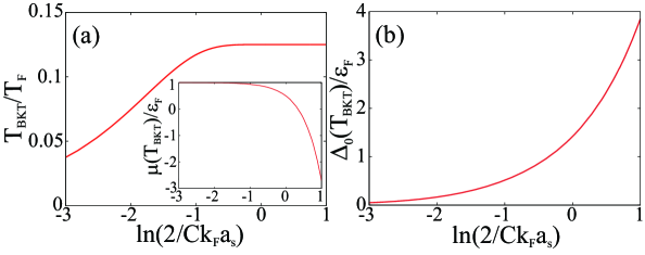
Figure 1: (a) Calculated BKT phase transition temperature $T_{\rm{BKT}}$. The inset shows the chemical potential $\mu(T_{\rm{BKT}})$. $T_{\rm F}$ is the Fermi temperature. (b) Saddle point solution (mean-field order parameter) $\Delta_{0}$ at $T_{\rm{BKT}}$, normalized by the Fermi energy $\varepsilon_{\rm F}$.

While the present formalism can describe strong-coupling effects in the normal state, it does not give the BKT instability. Thus, to determine $T_{\rm BKT}$, we employ the prescription used in Refs. [23, 24, 25]. Including phase fluctuations $\theta(x)$ around the saddle point solution $\Delta_{0}$ of the action $S_{\rm{eff}}$ in Eq. (3) ($\Delta(x)=\Delta_{0}e^{i\theta(x)}$) within the Gaussian fluctuations level, we obtain

$$\mathcal{Z}=e^{-S_{\rm{MF}}}\int\mathcal{D}[\theta]e^{-S_{\rm{FL}}},$$ (12)

where $S_{\rm{MF}}$ is given by Eq. (3) with $\Delta(x)$ being replaced by $\Delta_{0}$. $S_{\rm{FL}}=\sum_{\mathbf{q},i\nu_{n}}[Jq^{2}+K\nu_{n}^{2}]\theta(\mathbf{q},i\nu_{n})\theta(-\mathbf{q},-i\nu_{n})$ is the fluctuation contribution. Here,

$$J=\frac{1}{4m}\sum_{\mathbf{p}}\biggr{[}1-\frac{\xi_{\mathbf{p}}}{E_{\mathbf{p}}}{\rm{tanh}}\biggl{(}\frac{E_{\mathbf{p}}}{2T}\biggr{)}-\frac{1}{2T}\frac{p^{2}}{2m}{\rm sech}^{2}\biggl{(}{E_{\mathbf{p}}\over 2T}\biggr{)}\biggl{]}$$ (13)

is the phase stiffness, and $K=\frac{1}{4}\sum_{\mathbf{p}}\biggr{[}\frac{\Delta_{0}^{2}}{E_{\mathbf{p}}^{3}}{\rm{tanh}}\bigl{(}\frac{E_{\mathbf{p}}}{2T}\bigr{)}+\frac{1}{2T}\frac{\xi^{2}_{\mathbf{p}}}{E_{\mathbf{p}}^{2}}{\rm sech}^{2}\bigl{(}\frac{E_{\mathbf{p}}}{2T}\bigr{)}\biggr{]},$ where $E_{\mathbf{p}}=\sqrt{\xi^{2}_{\mathbf{p}}+\Delta^{2}_{0}}$. Using the phase stiffness constant $J$ in Eq. (13), we determine $T_{\rm BKT}$ from the KT-Nelson formula[28], $T_{\rm BKT}=(\pi/2)J(T_{\rm BKT})$. In this equation, $\Delta_{0}$ is determined from the BCS gap equation, $1=U\sum_{\mathbf{p}}{1\over 2E_{\mathbf{p}}}\tanh\bigl{(}{E_{\mathbf{p}}\over 2T}\bigr{)},$ and $\mu$ is evaluated from the number equation $N=-\partial\Omega/\partial\mu$, where $\Omega=-T\ln{\mathcal{Z}}$ with ${\mathcal{Z}}$ being given by Eq. (12) where the $\theta$-integration has been executed. Figure 1 shows the self-consistent solutions for $T_{\rm BKT}$, $\mu$, and $\Delta_{0}$.

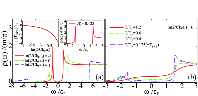
Figure 2: (a) Calculated density of states $\rho(\omega)$ at $T_{\rm BKT}$. The left inset shows the chemical potential $\mu$ used in this calculation. The right inset shows the BCS superfluid density of states, where the parameter set $(\Delta_{0},\mu)$ shown in Fig. 1 at $\ln(2/Ck_{\rm F}a_{\rm s})=0$ is used. (b) $\rho(\omega)$ at various temperatures when $\ln(2/Ck_{\rm F}a_{\rm s})=0$.

3 Pseudogap phenomenon near the BKT phase transition

Figure 2(a) shows the single-particle density of states $\rho(\omega)$ at $T_{\rm BKT}$. We see a clear gap-like structure even in the relatively weak-coupling case ($\ln(2/Ck_{\rm F}a_{\rm s})=-1$), which becomes more remarkable for a stronger interaction. We recall that, although we have introduced the saddle point solution $\Delta_{0}$ in calculating $T_{\rm BKT}$, this mean-field order parameter is not used in $\rho(\omega)$ in Eq. (11). Thus, the gap-like structure in Fig. 2(a) is the pseudogap associated with pairing fluctuations. Since the low-dimensionality enhances pairing fluctuations, the pseudogap in the present case is more remarkable than the three-dimensional case[19].

When $\ln(2/Ck_{\rm F}a_{\rm s})\geq 0$, the pseudogap structure at $T_{\rm BKT}$ is very similar to the BCS superfluid density of states with sharp coherence peaks at the gap edges (see the right inset in Fig. 2(a)). To understand this, we note that the particle-particle scattering matrix $\Gamma({\mathbf{q}},i\nu_{n})$ in Eq. (10), which describes fluctuations in the Cooper channel, would be large when ${\mathbf{q}}=\nu_{n}=0$ near $T_{\rm BKT}$. Using this, when we approximate Eq. (10) to $\Sigma({\mathbf{p}},i\omega_{n})\simeq G_{0}(\mathbf{-p},-i\omega_{n})T\sum_{\mathbf{q},i\nu_{n}}\Gamma({\mathbf{q}},i\nu_{n})\equiv-G_{0}(\mathbf{-p},-i\omega_{n})\Delta_{\rm PG}^{2}$, the Green’s function $G$ in Eq. (11) is found to have the same form as the ordinary particle component of the BCS Green’s function as,

$$G(\mathbf{p},i\omega_{n})=-\frac{i\omega_{n}+{\xi}_{\mathbf{p}}}{\omega_{n}^{2}+\xi_{\mathbf{p}}^{2}+\Delta_{\rm{PG}}^{2}}.$$ (14)

This means that the so-called pseudogap parameter $\Delta_{\rm PG}$[19, 29] plays similar roles to the BCS superfluid order parameter $\Delta_{0}$, leading to the pseudogap with sharp ‘coherence’ peaks, as shown in Fig. 2(a). Thus, when one measures $\rho(\omega)$ near $T_{\rm BKT}$, the system would look like the mean-field BCS state, although the superfluid order parameter $\Delta$ is actually absent and strong pairing fluctuations only exist.

While the pseudogap structure is similar to the BCS density of states at $T_{\rm BKT}$, their temperature dependence is very different from each other. In the BCS state, when the temperature increases, the gap width gradually becomes small, keeping the sharp coherence peaks at the gap edges, In contrast, Fig. 2(b) shows that the pseudogap structure, as well as the sharp peaks, gradually become obscure with increasing the temperature.

4 Summary

To summarize, we have discussed strong-coupling properties of a two-dimensional ultracold Fermi gas. Including pairing fluctuations within the framework of a Gaussian fluctuation theory, we calculated the single-particle density of states $\rho(\omega)$ near the BKT phase transition. At $T_{\rm BKT}$, pairing fluctuations induce a pseudogap in $\rho(\omega)$, the structure of which is very similar to the BCS superfluid density of states with a finite excitation gap, as well as sharp coherence peaks at the gap edges. That is, the BCS-like energy gap is expected to be observed even in a two-dimensional Fermi gas near $T_{\rm BKT}$, although the superfluid order parameter is absent and the system is dominated by low-dimensional pairing fluctuations. Since the achievement of the BKT phase transition is an exciting challenge in cold Fermi gas physics, our results would be useful for the study of this superfluid state on the view point of single-particle excitations.

We thank D. Inotani, R. Hanai, and H. Tajima for discussions. Y.O. was supported by a Grant-in-Aid for Scientific Research from MEXT in Japan (Grant No. 25105511 and No. 25400418).

5 References

References

- [1] Gurarie V and Radzihovsky L 2007 Ann. Phys. 332 2
- [2] Bloch I, Dalibard J and Zwerger W 2008 Rev. Mod. Phys. 80 885
- [3] Giorgini S, Pitaevskii L P and Stringari S 2008 Rev. Mod. Phys. 80 1215
- [4] Sommer A T, Cheuk L W, Ku M J H, Bakr W S and Zwierlein M W 2012 Phys. Rev. Lett. 108 045302
- [5] Regal C A, Greiner M and Jin D S 2004 Phys. Rev. Lett. 92 040403
- [6] Zwierlein M W, Stan C A, Schunck C H, Raupach S M F, Kerman A J and Ketterle W 2004 Phys. Rev. Lett. 92 120403
- [7] Kinast J, Hemmer S L, Gehm M E, Turlapov A and Thomas J E 2004 Phys. Rev. Lett. 92 150402
- [8] Bartenstein M, Altmeyer A, Riedl S, Jochim S, Chin C, Denschlag J H and Grimm R 2004 Phys. Rev. Lett. 92 203201
- [9] Feld M, Fröhlich B, Vogt E, Koschorreck M and Köhl M 2011 Nature 480 75
- [10] Fröhlich B, Feld M, Vogt E, Koschorreck M, Zwerger W and Köhl M 2011 Phys. Rev. Lett. 106 105301
- [11] Mermin N D and Wagner H 1966 Phys. Rev. Lett. 17 1133
- [12] Hohenberg P C 1967 Phys. Rev. 158 383
- [13] Berezinskii V L 1971 Sov. Phys. JETP 32 493
- [14] Berezinskii V L 1972 Sov. Phys. JETP 34 610
- [15] Kosterlitz J M and Thouless D J 1973 J. Phys. C:Solid State Phys. 6 1181
- [16] Hadzibabic Z, Krger P, Cheneau M, Battelier B and Dalibard J 2006 Nature 441 1118
- [17] Nozières P and Schmitt-Rink S 1985 J. Low Temp. Phys. 59 195
- [18] Sá de Melo C A R, Randeria M and Engelbrecht J R 1993 Phys. Rev. Lett. 71 3202
- [19] Tsuchiya S, Watanabe R and Ohashi Y 2009 Phys. Rev. A 80 033613
- [20] Pietilä V 2012 Phys. Rev. A 86 023608
- [21] Watanabe R, Tsuchiya S and Ohashi Y 2013 Phys. Rev. A 88 013637
- [22] Klimin S N, Tempere J and Devreese J T 2012 New J. Phys. 14 103044
- [23] Iskin M and Sá de Melo C A R 2009 Phys. Rev. Lett. 103 165301
- [24] Tempere J, Klimin S N and Devreese J T 2009 Phys. Rev. A 79 053637
- [25] Salasnich L, Marchetti P A and Toigo F 2013 Phys. Rev. A 88 053612
- [26] Morgan S A, Lee M D and Burnett K 2002 Phys. Rev. A 65 022706
- [27] When the Green’s function in Eq. (9) is used in Eq. (11), the resulting density of states is known to unphysically become negative in the strong-coupling region[19]. This difficulty is, however, avoided by using . We note that the Green’s function with the self-energy given by Eq. (10) is the same as that in the -matrix approximation[19].
- [28] Nelson D R and Kosterlitz J M 1977 Phys. Rev. Lett. 39 1201
- [29] Chen Q J and Levin K 2009 Phys. Rev. Lett. 102 190402