Prioritized Data Compression using Wavelets

Abstract

The volume of data and the velocity with which it is being generated by computational experiments on high performance computing (HPC) systems is quickly outpacing our ability to effectively store this information in its full fidelity. Therefore, it is critically important to identify and study compression methodologies that retain as much information as possible, particularly in the most salient regions of the simulation space. In this paper, we cast this in terms of a general decision-theoretic problem and discuss a wavelet-based compression strategy for its solution. We provide a heuristic argument as justification and illustrate our methodology on several examples. Finally, we will discuss how our proposed methodology may be utilized in an HPC environment on large-scale computational experiments.

Keywords: Wavelets, Data Compression, High Performance Computing

1 Introduction

The US Department of Energy recently published a document highlighting several issues related to data-intensive computing on future high-performance computing (HPC) systems [5] with particular emphasis given to data analysis and visualization in Chapter 4. The authors highlight the growing disparity between I/O and storage capabilities, and computational capabilities. They warn that “our ability to produce data is rapidly outstripping our ability to use it”, particularly in a meaningful manner. This statement echoes the sentiments expressed in previous DOE publications, e.g. Ahern et al., [1], Ashby et al., [2], among others. The problem has recently manifested itself at the National Renewable Energy Laboratory in the form of large-scale wind-turbine array simulations. That is, data analysis tools and the computational machinery that supports them have not been able to scale with the HPC systems that are generating the wind-turbine array simulations.

These considerations motivate the following research on what we term a prioritized wavelet-based data compression methodology. We propose storing data in varying fidelities within the simulation space based on regions of saliency. That is, salient regions will be stored in a high fidelity whereas the less important regions will be more compressed. As an example, one might imagine the area directly in the wake of a wind turbine as being more important in future analysis/visualization experiments and, thus, we would like to retain the simulated data in its fullest fidelity in these regions. On the other hand, data on the periphery of the wind farm (less turbulent) might be less interesting from a subsequent analytic perspective, and may be stored in a lower fidelity in order to save space.

The wavelet representation of a signal has a history of use in both data compression and denoising [13]. The two applications use the same basic algorithm of (1) performing a discrete wavelet transform, (2) setting all coefficients in the representation whose magnitude is below a threshold to zero, and then (3) reconstructing the signal based on the sparse wavelet representation. Wavelet compression has most commonly been used for images [14] and time-series such as electrocardiogram signals [12].

Optimal data compression sensitive to secondary analysis has not been generally investigated, though there are some specific applications in image processing. While not framed as an explicit secondary analysis, there have been algorithms created to find optimal compression of an image sensitive to human visual perception (see for example [4] or the JPEG-2000 standards [14]). We presume in our methodology that the form of secondary analysis can be expressed explicitly as a mathematical function on the data, however we expect the approach taken here may be extended to include more loosely defined secondary analyses.

The use of wavelet-based compression schemes is becoming increasingly popular in the data visualization domain, see for example Gruchalla, [9], Gruchalla et al., [10], and Gruchalla et al., [11]. We fully expect this trend to continue with their inclusion as the default compression tool in the VAPOR software package [6]. One of our aims with this research is to develop a compression strategy that allows for heterogeneous levels of compression throughout the simulation domain while remaining consistent with VAPOR’s use of the discrete wavelet transform.

While our current work does not address the motivating problem per se ( compression strategies for exascale-type problems), our intentionally narrow focus provides the foundation upon which future research may be built. We lay out the mathematical background, our current problem of interest, and provide a heuristic justification for our proposed solution in Section 2. We illustrate the novel approach on several examples in Section 3. Finally, in Section 4, we summarize our results and discuss future research directions as they relate to problems in HPC environments.

2 Notation/Formulation

2.1 Brief Introduction to Wavelets

The notion of a wavelet is suggested by the name. They are ‘little waves’, in the sense that they possess some quality of oscillation, but have small, localized support. A single wavelet is one member of a complete set of basis functions with which we can represent a time series or, in general, a function. Though there are many such sets of basis functions which qualify as wavelets, it is useful to consider a particular set widely considered to be the simplest. The wavelets which make up this set are called Haar wavelets, and they are defined by translations and dilations of the so called mother Haar wavelet defined as

$$\psi(t) =\begin{cases}1\;&t\in\left[0,\frac{1}{2}\right)\\ -1&t\in\left[\frac{1}{2},1\right)\\ 0&\text{otherwise}.\end{cases}$$

By choosing $j$ and $k$ appropriately, we can build a complete basis which spans $L^{2}(\mathbb{R})$, and thus represent all square integrable functions as linear combinations of these wavelets

$$\psi_{j,k}(t) =2^{j/2}\psi(2^{j}t-k)$$

with time series representation

$$f(t) =\sum_{j}\sum_{k}a_{j,k}\psi_{j,k}(t).$$

These equations describe the continuous wavelet transform, but there are analogous forms for discrete representations as well. For a more thorough introduction to wavelets, see [13].

These basis functions are useful for many reasons, including the fact that the wavelet representation is relatively efficient to compute, and the representation is robust in the presence of discontinuities compared to related methods. Additionally, the Haar wavelet is a member of a class of wavelets which form an orthonormal basis and provides the following useful form

$$\sum_{t=1}^{n}f^{2}(t) =\sum_{k}\sum_{j}a^{2}_{j,k}.$$ (1)

This identity, sometimes referred to as Parseval’s relation, serves as the foundation for a class of estimators $\hat{\boldsymbol{f}_{B}}$ that we propose in Section 2.3.

2.2 Decision-Theoretic Prioritization

This formulation considers the situation where the secondary analysis to be performed upon $\boldsymbol{f}=\left(f(1),\dots,f(n)\right)^{\prime}$, some finite vector of data indexed by $t=1,\dots,n$, may be explicitly expressed as a transformation $\mathbf{g}\!:\!\mathbb{R}^{n}\rightarrow\mathbb{R}^{m}$. The flexible nature of $\mathbf{g}$ gives this procedure a wide range of applicability. Take for example the following hypothetical situation.

Example 2.1 (Moments).

Suppose we have data $\boldsymbol{f}$ for which we want to estimate the first four moments. Our secondary function then is given by the following map from $\mathbb{R}^{n}$ to $\mathbb{R}^{4}$:

$$\mathbf{g}(\boldsymbol{f})=\mathbf{g}(f(1),\dots,f(n)) =\left(\sum_{t=1}^{n}f(t),\;\sum_{t=1}^{n}f^{2}(t),\;\sum_{t=1}^{n}f^{3}(t),\;\sum_{t=1}^{n}f^{4}(t)\right)^{\prime}.$$

We will use the notation $g_{i}(\boldsymbol{f})$ to refer to a single component of the vector $\mathbf{g}(\boldsymbol{f})$, for example

$$g_{i}(\boldsymbol{f})=\sum_{t=1}^{n}f^{i}(t),\quad i=1,\dots,4.$$

We will revisit this particular example in Example 3.4 in Section 3.

We suppose now that storing the full-fidelity data $\boldsymbol{f}$ is impractical, and we will instead be forced to make do with $\hat{\boldsymbol{f}}$, a compressed version of $\boldsymbol{f}$, which for the moment need not be wavelet-based. In order to give some simple but meaningful measure to the amount of error in $\hat{\boldsymbol{f}}$, and $\mathbf{g}(\hat{\boldsymbol{f}})$, we propose modeling the errors $\hat{\boldsymbol{f}}-\boldsymbol{f}$ as a random vector generated from some distribution with mean $\mathbf{0}$ and covariance matrix $\boldsymbol{\Sigma}$. In fact, for the case of wavelet-based compression, each $\hat{f}(t)-f(t)$ will not be random, but entirely deterministic. For even moderately large $n$ though, these values may behave similarly to random variables. By modeling the errors in this way, we are able to develop this problem from a decision-theoretic perspective [3] and minimize the expected squared distance between $\boldsymbol{\theta}=\mathbf{g}(\boldsymbol{f})$ and a candidate estimator $\hat{\boldsymbol{\theta}}=\mathbf{g}(\hat{\boldsymbol{f}})$. Specifically, we use the squared error loss function

$$L(\boldsymbol{\theta},\boldsymbol{a}) =\left(\boldsymbol{\theta}-\boldsymbol{a}\right)^{\prime}\left(\boldsymbol{\theta}-\boldsymbol{a}\right)=||\boldsymbol{\theta}-\boldsymbol{a}||_{2}^{2}$$ (2)

with corresponding risk for a candidate estimator $\boldsymbol{\delta}$ defined by

$$R(\boldsymbol{\theta},\boldsymbol{\delta}) =\mathbb{E}\left[L(\boldsymbol{\theta},\boldsymbol{\delta})\right].$$

Note that we are operating under the constraint that all candidate approximations, $\hat{\boldsymbol{f}}$, must be of the same fixed size, where size will be a measure of the total cost of storing the approximation $\hat{\boldsymbol{f}}$. In the case of wavelet-based compression, this is defined to be the number of non-zero wavelet coefficients. For complicated $\mathbf{g}$, $\boldsymbol{f}$, and approximations $\hat{\boldsymbol{f}}$, it may be an extremely intensive or even impossible computation to find the optimal such $\hat{\boldsymbol{f}}$. We therefore impose two limitations. First, we will require that we be able to linearize $\mathbf{g}$ and use the first-order Taylor approximation:

$$\mathbf{g}(\hat{\boldsymbol{f}})-\mathbf{g}(\boldsymbol{f}) \approx J_{\mathbf{g}}\cdot(\hat{\boldsymbol{f}}-\boldsymbol{f}).$$

where $J_{\mathbf{g}}$ is the $m\times n$ Jacobian matrix whose $i,t$ element is $\partial g_{i}(\boldsymbol{f})/\partial f(t)$, and $i=1,\dots,m$, $t=1,\dots,n$. Second, we limit ourselves to a subset of the class of all fixed-size $\hat{\boldsymbol{f}}$, defined in Section 2.3. This class is defined such that approximations are relatively easy to compute, but still flexible enough in their structure to take into account the demands of the specific secondary analysis $\mathbf{g}$.

2.3 A class of ‘magnifying glass’ approximations $\hat{\boldsymbol{f}}_{B}$

From now on, $\hat{\boldsymbol{f}}$ will refer to an estimator made through (1) generating a wavelet transform of $\boldsymbol{f}$, (2) setting a fixed number of coefficients to zero, and then (3) reconstructing $\hat{\boldsymbol{f}}$ with this sparse wavelet representation. The class we propose yields estimators which are practically straightforward to produce, are mathematically tractable, and yield estimators with significant improvements compared to a natural baseline estimator $\tilde{\boldsymbol{f}}$. The baseline estimator is what would be produced if we completely ignored the secondary function $\mathbf{g}$, and instead followed the wavelet compression procedure which minimized the squared error norm $||\tilde{\boldsymbol{f}}-\boldsymbol{f}||^{2}_{2}$ (where $\tilde{\boldsymbol{f}}$ is taken to be the same size as $\hat{\boldsymbol{f}}_{B}$). See the top plot in Figure 1 for one example.

First, we write the general $\hat{\boldsymbol{f}}$ with errors partitioned into two disjoint sets $B$ and $B^{c}$ whose union is the indexing set $T=\left\{1,\dots,n\right\}$. The $t^{th}$ element may be written as

$$\hat{f}_{B}(t) =f(t)+\varepsilon_{B}(t)\mathbf{1}_{B}(t)+\varepsilon_{B^{c}}(t)\mathbf{1}_{B^{c}}(t)$$

where $\mathbf{1}_{B}(t)$ is the usual indicator function equal to one if $t\in B$ and zero otherwise. Our class of $\hat{\boldsymbol{f}}_{B}$ will be those for which the mean squared error in $B$ is proportional to the mean squared error in $B^{c}$. That is, we define

$$\sigma^{2}_{B} :=|B|^{-1}\sum_{t\in B}\varepsilon_{B}^{2}(t),\ \text{and}$$

$$\sigma^{2}_{B^{c}} =\frac{1}{\kappa}\sigma^{2}_{B}$$ (3)

where $|B|=$ the number of elements in $B$.

We can easily generate $\hat{\boldsymbol{f}}_{B}$ such that (3) holds (to a high level of precision) when we have orthonormal wavelets, and the set $B$ is made up of a small number of connected intervals in $T$. The reason we need $B$ to be this sort of set is so that we can make use of the compact support of our wavelets. In our toy examples we only use the Haar wavelet, but the procedure by which we generate $\hat{\boldsymbol{f}}_{B}$ may be extended to any orthonormal wavelet basis with minor modifications. We use the localized nature of the Haar wavelet basis functions along with (1) in the following way.

First, we define a set $\mathcal{B}$, which is a set indexing all wavelet basis functions whose support overlaps the region $B\in T$. We then order from smallest to largest the coefficients of the wavelets in $\mathcal{B}$ and ${\mathcal{B}}^{c}$ by their squared value

$$(a^{2}_{\mathcal{B}(1)},\dots,a^{2}_{\mathcal{B}(n_{J})}),\text{ and }(a^{2}_{\mathcal{B}^{c}(1)},\dots,a^{2}_{\mathcal{B}^{c}(n_{L})})$$

and choose the unique pair of threshold values $\alpha^{2}_{\mathcal{B}}$ and $\alpha^{2}_{\mathcal{B}^{c}}$ so that

$$n^{-1}_{J}\sum_{a^{2}_{\mathcal{B}(j)}<\alpha^{2}_{\mathcal{B}}}a^{2}_{\mathcal{B}(j)} =\kappa n^{-1}_{L}\sum_{a^{2}_{\mathcal{B}^{c}(l)}<\alpha^{2}_{\mathcal{B}^{c}}}a^{2}_{\mathcal{B}^{b}(l)}.$$ (4)

The values $\alpha^{2}_{\mathcal{B}}$ and $\alpha^{2}_{\mathcal{B}^{c}}$ are unique because we have fixed the number of non-zero coefficients.

Because of the localized support of the wavelets, when $B$ is made up of a small number of connected subsets of $T$, the number of wavelets with support in both $B$ and $B^{c}$ will be small compared to the number of wavelets with support entirely in $B$ or $B^{c}$. Moreover, the coefficients which typically have small magnitudes are those which correspond to basis functions at finer scales, which means the wavelet coefficients which are most likely to be effected by thresholding are the ones who tend to have support entirely in $B$ or $B^{c}$. Therefore we will have $|B|\approx n_{J}$ and also

$$\frac{1}{|B|}\sum_{t\in B}(\hat{f}_{B}(t)-f(t))^{2} \approx\frac{1}{n_{J}}\sum_{a^{2}_{\mathcal{B}(j)}<\alpha^{2}_{\mathcal{B}}}a^{2}_{\mathcal{B}(j)}$$

as well as the analogous result for $B^{c}$ and $\mathcal{B}^{c}$. Therefore, ensuring (4) in turn ensures that (3) approximately holds. In practice, when we implemented this procedure, we were able to generate $\hat{\boldsymbol{f}}_{B}$ for which $\hat{\kappa}$, the realized value of the ratio of mean squared errors, came very close to $\kappa$. When we specified $\kappa=0.1$, for example, our realized ratio was generally in $(0.09,0.11)$.

These $\hat{\boldsymbol{f}}_{B}$ are in some sense the simplest possible way to take into account the demands of the secondary analysis. We are partitioning the indexing set $T$ into two subsets, where values $f(t)$, $t\in B$ are more important than values $f(t^{*})$, $t^{*}\notin B$ in accurately estimating $\mathbf{g}(\boldsymbol{f})$ by a factor of $\kappa$. Therefore, a datum $f(t)$ is either important or not important, there is no spectrum of importance. Familiarly, we call these approximations $\hat{\boldsymbol{f}}_{B}$ ‘magnifying glass’ estimators with magnification factor $\kappa^{-1}$ since they effectively give us a closer look at region $B$ compared to $B^{c}$ (see bottom plot of Figure 1). More subtle schemes are certainly worth investigating, but this first-order approach already yields promising results.

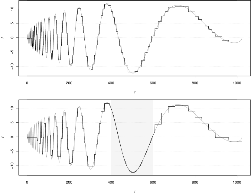
Figure 1: The top plot shows the full fidelity time series in gray (‘Doppler’) with the baseline wavelet-based approximation in black. This approximation ignores the secondary analysis. The bottom plot shows the same time series in gray with an approximation $\hat{\boldsymbol{f}}_{B}$ in black. In this example, $\kappa$ was set at 0.02, with realized value $\hat{\kappa}=0.0209$, and $B=\{401,\dots,600\}$ (inducated in both plots by the light shading). We set the size of this approximation so that only 10% of the wavelet coefficients were non-zero. The ‘magnifying glass’ approximation is noticeably closer to the truth in $B$ than in $B^{c}$.

Figure 1 shows an implementation of this method. In the top plot, the gray curve shows the full-fidelity time series (‘Doppler’ [13]) and the black step function is the baseline approximation $\tilde{\boldsymbol{f}}$. In the bottom plot, the gray curve is the same, but the approximation shown is a magnifying glass estimator with $B=\{401,\dots,600\}$ and $\kappa=0.02$ ($\hat{\kappa}=0.0209$). The size of the approximation is such that 10% of the wavelet coefficients were allowed to be non-zero. The higher fidelity region appears to extend slightly beyond $B$ on both ends because of the presence of wavelet basis functions with overlapping support.

The values $\sigma^{2}_{B}$ and $\sigma^{2}_{B^{c}}$ will depend both on $\kappa$ and the size of the approximation. For instance, the smallest possible $\sigma^{2}_{B}$ and $\sigma^{2}_{B^{c}}$ for a given approximation size will occur when $\kappa=1$. As $\kappa$ decreases toward 0, we are sacrificing some overall increase in the error in $\hat{\boldsymbol{f}}_{B}$ in exchange for better estimating the parts of $\boldsymbol{f}$ that are most important for the secondary analysis $\mathbf{g}$, resulting in an overall improvement in the precision of $\mathbf{g}(\hat{\boldsymbol{f}}_{B})$.

2.4 Importance Function

In order to add some degree of saliency to regions within the simulation space, we introduce the ‘importance function’ concept. Recall the loss function defined in 2 and note that it can be re-written (approximately) as

$$L(\mathbf{g},\hat{\boldsymbol{f}}) \approx\left[J_{\mathbf{g}}\cdot(\hat{\boldsymbol{f}}-\boldsymbol{f})\right]^{\prime}\left[J_{\mathbf{g}}\cdot(\hat{\boldsymbol{f}}-\boldsymbol{f})\right]$$

$$=(\hat{\boldsymbol{f}}-\boldsymbol{f})^{\prime}J_{\mathbf{g}}^{\prime}J_{\mathbf{g}}(\hat{\boldsymbol{f}}-\boldsymbol{f})$$

$$=(\hat{\boldsymbol{f}}-\boldsymbol{f})^{\prime}\mathbf{M}(\hat{\boldsymbol{f}}-\boldsymbol{f}).$$

We will refer to $\mathbf{M}:=J_{\mathbf{g}}^{\prime}J_{\mathbf{g}}$ as the ‘importance matrix’ and its diagonal elements as the ‘importance function’. This name will become clear later when we show that the diagonal of this matrix largely determines the form of the optimal approximation. These $n$ diagonal elements can be thought of as defining a level of importance or weight for each datum $f(t)$.

We will now model the deterministic errors $\hat{\boldsymbol{f}}-\boldsymbol{f}$ as a random vector with mean vector $\mathbf{0}$ and covariance matrix $\boldsymbol{\Sigma}$. For approximations of type $\hat{\boldsymbol{f}}_{B}$, a natural covariance matrix to ascribe to this random variable is a diagonal matrix with elements equal to either $\kappa\sigma^{2}_{B^{c}}$ or $\sigma^{2}_{B^{c}}$. Using this model, our loss function takes a quadratic form, and the risk is approximated by

$$R(\mathbf{g},\hat{\boldsymbol{f}}_{B}) \approx\mathbb{E}\left[(\hat{\boldsymbol{f}}-\boldsymbol{f})^{T}\mathbf{M}(\hat{\boldsymbol{f}}-\boldsymbol{f})\right]$$

$$=\text{tr}(\mathbf{M}\Sigma)$$

$$=\sigma^{2}_{B^{c}}\left[\kappa\sum_{t\in B}\sum_{i=1}^{m}\left(\frac{\partial g_{i}}{\partial f(t)}\right)^{2}+\sum_{t\notin B}\sum_{i=1}^{m}\left(\frac{\partial g_{i}}{\partial f(t)}\right)^{2}\right].$$ (5)

In order to minimize $R(\mathbf{g},\hat{\boldsymbol{f}}_{B})$, we will need to take into account two effects determined by $B$. First, as the size of $B$ increases, $\sigma^{2}_{B^{c}}$ will increase, since more and more error in $B^{c}$ will be sacrificed to maintain the higher fidelity in $B$. Second, the choice of $B$ will have an impact on the two sums. If we choose $B$ such that the largest values of $\sum_{i=1}^{m}\left(\partial g_{i}/\partial f(t)\right)^{2}$ are in the first term of Equation (5), then we will reduce our risk function $R(\mathbf{g},\hat{\boldsymbol{f}}_{B})$ because $\kappa<1$. Taking these together, we can intuitively expect that the optimal set $B$ will be the smallest possible set such that the large elements on the diagonal of $\mathbf{M}$ have index inside $B$.

2.5 Idealized Secondary Analysis

We now turn our attention to one idealized setting where the secondary analysis takes a contrived form as a basic check on casting the problem in this decision-theoretic manner. Consider the following secondary calculation $\mathbf{g}$ defined by

$$\mathbf{g}(\boldsymbol{f})_{i} :=f(i)(\lambda\mathbf{1}_{A}(i)+\mathbf{1}_{A^{c}}(i)),\quad i=1,\dots,n$$

or written more explicitly

$$g_{i}(\boldsymbol{f}) =\begin{cases}\lambda f(i),\quad&i\in A\\ f(i),&i\notin A\end{cases}$$

$$i \in\{1,\dots,1024\}.$$

This represents the case where our secondary analysis consists merely of multiplying some elements of $\boldsymbol{f}$ by a scalar $\lambda$, and retaining the rest unaltered. This is akin to placing some region of the data under a magnifying glass with a magnification factor of $\lambda$, and we therefore expect an estimator of type $\hat{\boldsymbol{f}}_{B}$ to be a good choice. For $\lambda$ greater than one, we expect that the optimal approximation $\hat{\boldsymbol{f}}_{B}$ ought to be one where $B\approx A$, since this is clearly the ‘important’ part of $\boldsymbol{f}$. The importance matrix is straightforward to calculate, since it is the product of two diagonal matrices with elements equal to either $\lambda$ or 1 depending on the index’s membership in $A$.

In the argument that follows, we let $\lambda$ go to infinity, and $\kappa$ go to zero, which corresponds to the case where $\mathbf{g}$ and $\boldsymbol{f}$ show infinite preference for region $A$ and $B$ respectively. In this extreme we will see that it is possible to verify $B=A$.

Starting from (5) we have

$$R(\mathbf{g},\hat{\boldsymbol{f}}_{B}) =\sigma^{2}_{B^{c}}\left[\kappa\left(\sum_{t\in A\cap B}\lambda^{2}+\sum_{t\in A^{c}\cap B}1\right)+\left(\sum_{t\in A\cap B^{c}}\lambda^{2}+\sum_{t\in A^{c}\cap B^{c}}1\right)\right]$$

$$=\sigma^{2}_{B^{c}}\left[\kappa\left(\lambda^{2}|A\cap B|+|A^{c}\cap B|\right)+\lambda^{2}|A\cap B^{c}|+|A^{c}\cap B^{C}|\right].$$

As $\lambda$ approaches infinity, the risk will also become infinite, so we next normalize by the constant $\lambda^{2}$ to get

$$\frac{R(\mathbf{g},\hat{\boldsymbol{f}}_{B})}{\lambda^{2}} =\sigma^{2}_{B^{c}}\left[\kappa\left(|A\cap B|+\frac{|A^{c}\cap B|}{\lambda^{2}}\right)+|A\cap B^{c}|+\frac{|A^{c}\cap B^{c}|}{\lambda^{2}}\right].$$ (6)

Minimizing (6) is equivalent to minimizing the risk, but now as we let $\lambda^{2}$ grow large, the quantity of interest simplifies to

$$\lim_{\lambda^{2}\rightarrow\infty}\left(\frac{R(\mathbf{g},\hat{\boldsymbol{f}}_{B})}{\lambda^{2}}\right) =\sigma^{2}_{B^{c}}\left(\kappa|A\cap B|+|A\cap B^{c}|\right).$$ (7)

To get any further, we need to know more about how $\sigma^{2}_{B^{c}}$ depends on our choice of $B$. In practice, this relationship will be complicated, but roughly speaking we expect $\sigma^{2}_{B^{c}}$ to be monotone increasing as $|B|$ increases as discussed in Section 2.4 (see Figure 2). From (7), we can see that the second factor in the limiting risk is independent of the size of $A^{c}\cap B$, and so we might as well choose $B^{\prime}=A\cap B$ instead of $B$. That is,

$$\lim_{\lambda^{2}\rightarrow\infty}\left(\frac{R(\mathbf{g},\hat{\boldsymbol{f}}_{B})}{\lambda^{2}}\right) \geq\lim_{\lambda^{2}\rightarrow\infty}\left(\frac{R(\mathbf{g},\hat{\boldsymbol{f}}_{A\cap B})}{\lambda^{2}}\right),$$

since $\sigma^{2}_{B^{c}}$ is monotone increasing in $|B|$. It is clear the optimal $B$ will be contained within $A$.

Letting $\kappa$ go to zero now yields

$$\lim_{\lambda^{2}\rightarrow\infty,\;\kappa\rightarrow 0}\left(\frac{R(\mathbf{g},\hat{\boldsymbol{f}}_{B})}{\lambda^{2}}\right) =\sigma^{2}_{B^{c}}|A\cap B^{c}|.$$

Now as $B$ increases in size to approach $B=A$, $\sigma^{2}_{B^{c}}$ will increase, but when $B=A$, the second term is zero and the normalized risk vanishes. We will see in Examples 3.1 and 3.2 that even when $\lambda$ and $\kappa$ are far from infinity and zero, this result still holds to large degree.

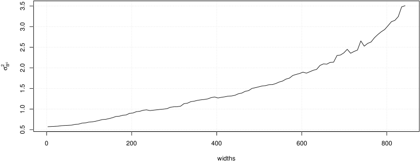
Figure 2: This plot shows the roughly monotone behavior of $\sigma^{2}_{B^{c}}$ as we increase the size of $B$ for fixed $\kappa=0.1$. In this case, we used the ‘Doppler’ time series and let $B$ increase from $\{511,512,513\}$ to $\{91,\dots,931\}$, increasing the width by 4 in each direction at each step. The units on the $y$-axis are specific to this example, but the monotone behavior is generally applicable.

3 Examples

In considering possible sets $B\subset T$, it is computationally intractable to consider all $2^{|T|}$ possible subsets. Often though, we may have reason to believe a priori that the most important parts of $\boldsymbol{f}$ lie predominantly in a few connected subsets of the space $T$. For instance, if the data are spatially or temporally arranged, we may expect strong positive correlation in importance between neighboring data. In our motivating example related to wind turbine arrays, we expect that the most important regions are in and around the wakes. In the following examples we restrict the space of possible $\hat{\boldsymbol{f}}_{B}$ to include only those for which $B$ is a single connected interval in $T$.

We performed a nearly-exhaustive (see Appendix A) search for the optimal $B$ for several toy examples. In each example our data $\boldsymbol{f}$ is one of two different one-dimensional time series, both widely used in simulation studies involving denoising and density estimation ([8] and [7]), and also used for illustration in [13]. In each case we also specify a secondary analysis $\mathbf{g}$, and a value for $\kappa$. In all examples, the size of the approximation is such that 10% of the wavelet coefficients were allowed to be non-zero. The nearly-exhaustive search considers almost all possible uninterrupted intervals within $T=\{1,\dots,1024\}$ for a fixed value $\kappa$. For each interval, the relative squared error is defined as

$$SE_{B} =L(\mathbf{g},\hat{\boldsymbol{f}}_{B}),$$

$$SE_{0} =L(\mathbf{g},\tilde{\boldsymbol{f}}),\&$$

relSE $$:=SE_{B}/SE_{0}.$$

Therefore, values of relSE less than 1 represent improvements over the baseline wavelet compression, $\tilde{\boldsymbol{f}}$, which ignores the secondary function. The interval corresponding to the smallest relSE is (nearly) optimal in the space of single uninterrupted intervals.

Example 3.1 (Idealized Secondary Analysis for ‘Doppler’ Time Series).

We offer here the results of implementation on a particular example of the idealized case mentioned in Section 2.5. For demonstration, the secondary function is

$$\mathbf{g}_{1}(\boldsymbol{f})_{i} =f(i)\left[5\times\mathbf{1}_{\{401,\dots,600\}}(i)+\mathbf{1}_{\{401,\dots,600\}^{c}}(i)\right],\quad i=1,\dots,n$$

so that $\lambda=5$ and $A=\{401,\dots,600\}\subset T=\{1,\dots,1024\}$. We therefore expect that the optimal $\hat{\boldsymbol{f}}_{B}$ will occur when $B\approx\{401,\dots,600\}$. Figure 3 shows the results of a nearly-exhaustive search over all single intervals $B$ in $T$ with fixed $\kappa=1/10$ for our first time series (‘Doppler’). The top plot is the full fidelity time series $\boldsymbol{f}$, with results overlaid. The bottom plot shows the importance function ($\text{diag}(\mathbf{M})$) with results overlaid. Each overlaid segment represents a proposed interval $B$, plotted at a height proportional to relSE, the ratio of squared error in $\hat{\boldsymbol{f}}_{B}$ to $\tilde{\boldsymbol{f}}$, the approximation which ignores $\mathbf{g}$. The axis to the right shows these relSE. Since this search procedure is naive, many of the proposed $\hat{\boldsymbol{f}}_{B}$ are in fact much worse than $\tilde{\boldsymbol{f}}$. We have included only the top performing $B$, in this case the top 2%.

The interval with the smallest relSE is $\{413,\dots,597\}$, which is almost exactly equal to the interval where the diagonal of $\mathbf{M}$ is large. As we saw in Figure 1, our method for generating $\hat{\boldsymbol{f}}_{B}$ tends to produce an approximation to $\boldsymbol{f}$ in which the high fidelity region bleeds slightly beyond the specified $B$, which may explain why the optimal interval is slightly narrower than we expected. Additionally, we can see in the bottom plot that the top 2% of intervals are all stably located near $\{401,\dots,600\}$, and this can be verified for a range of $\kappa$ values (we verified $\kappa=(1/5,1/10,1/20)$. In fact, this stability is visible well beyond the top 2% of relSE, but plots including a larger proportion of proposed segments are cluttered and difficult to interpret.

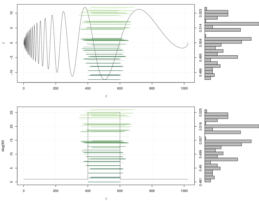
Figure 3: Top 2% of $B$ for the ‘Doppler’ time series and secondary function $\mathbf{g}_{1}$ in Example 3.1. Each horizontal line segment represents an interval $B$, and the height of each segment is proportional to the improvement over the approximation which ignores secondary analysis, $\tilde{\boldsymbol{f}}$. The ratio of squared error loss for $\hat{\boldsymbol{f}}_{B}$ to that of $\tilde{\boldsymbol{f}}$ is shown in the right axis. The histogram to the right of each plot shows the distribution of the top 2% of proposed intervals. Some segments $B$ have the same relSE, so the histogram helps to illuminate where segments have overlapped.

Example 3.2 (Idealized Secondary Analysis for ‘Doppler’ Time Series).

In this example, we keep the same secondary analysis $\mathbf{g}_{1}$, but we examine a different time series called ‘Bumps’. Figure 4 shows the same pair of plots as in Figure 3 for this new time series. It is interesting to note the influence here of not just the importance function, but also the nature of $\boldsymbol{f}$, in particular the places where the time series is equal to zero. In these regions, the approximation that the errors $\hat{\boldsymbol{f}}-\boldsymbol{f}$ are randomly distributed with variance $\sigma^{2}_{B}$ or $\sigma^{2}_{B^{c}}$ is unreasonable. Since it is trivial to represent data that are identically zero, the errors here will be zero for any reasonably sized approximation, i.e., for any approximation with more than a very small number of non-zero wavelet coefficients), regardless of our specification of $\kappa$. The optimal interval is $\{405,\dots,461\}$. As is visible in the top plot, this region corresponds roughly to the portion of $A$ where $\boldsymbol{f}$ is non-zero.

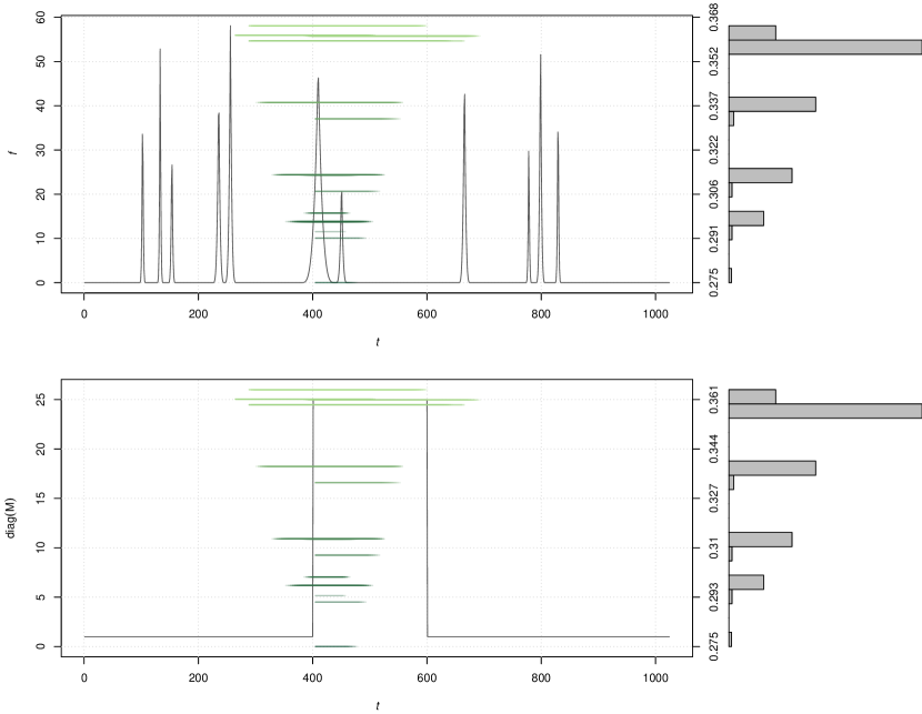
Figure 4: Top 5% of $B$ for the ‘Bumps’ time series and secondary function $\mathbf{g}_{1}$ in Example 3.2. Each horizontal line segment represents an interval $B$, and the height of each segment is proportional to the improvement over the approximation which ignores secondary analysis, $\tilde{\boldsymbol{f}}$. The ratio of squared error loss for $\hat{\boldsymbol{f}}_{B}$ to that of $\tilde{\boldsymbol{f}}$ is shown in the right axis. The histogram to the right of each plot shows the distribution of the top 2% of proposed intervals. Some segments $B$ have the same relSE, so the histogram helps to illuminate where segments have overlapped. In this example, it is interesting to note the influence of not just the importance function $\text{diag}(\mathbf{M})$, but also the nature of the data $\boldsymbol{f}$ themselves. In particular, there are many indices for which the data are close to zero. The optimal interval (most easily seen on the middle figure) is $\{405,\dots,461\}$, which corresponds roughly to the portion of $A$ where $\boldsymbol{f}$ is non-zero.

Example 3.3 (Exponential Sine).

We next consider a secondary analysis for which we will have little intuition. The function $\mathbf{g}$ is still chosen to be a map to $\mathbb{R}^{n}$, but the function is more complicated than the magnifying glass situation. We define the secondary analysis to be

$$\mathbf{g}_{3}(\boldsymbol{f})_{i} =e^{f(i)/6}\sin\left(f(i)\right),\quad i=1,\dots,n.$$

The shape of the importance function is now something more complicated than the function in the previous two examples. Without looking at the importance function, it is difficult to guess a priori where the most ‘important’ data will be, and where the lens of our magnifying glass approximation should lie. In this example we reuse the ‘Doppler’ data.

Figure 5 shows results overlaying the data (top) and the importance function (bottom). The best proposed intervals $B$ cover the region of the importance function where there are the most large values. Though the importance function attains large values in the interval $\{600,\dots,900\}$ as well as in the interval $\{350,\dots,425\}$, the former has more such values, and since we are only considering $B$ that are single intervals, it makes sense that the best $B$ are clustered more or less in this range.

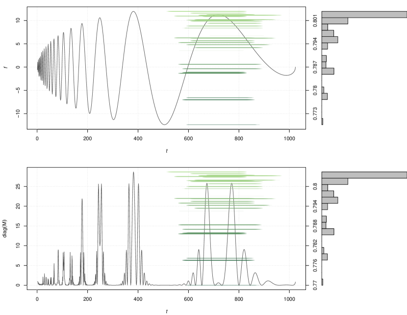
Figure 5: Top 5% of $B$ for the ‘Doppler’ time series and secondary function $\mathbf{g}_{3}$ in Example 3.3. Each horizontal line segment represents an interval $B$, and the height of each segment is proportional to the improvement over the approximation which ignores secondary analysis, $\tilde{\boldsymbol{f}}$. The ratio of squared error loss for $\hat{\boldsymbol{f}}_{B}$ to that of $\tilde{\boldsymbol{f}}$ is shown in the right axis. The histogram to the right of each plot shows the distribution of the top 2% of proposed intervals. Some segments $B$ have the same relSE, so the histogram helps to illuminate where segments have overlapped.

Example 3.4 (Moment estimators).

We consider one final secondary analysis on the ‘Doppler’ data, first mentioned in Example 2.1. In this example, we consider a secondary analysis that summarizes the raw data using the first four moments

$$\mathbf{g}_{4}(\boldsymbol{f}) =\left(\sum_{t}f(t),\sum_{t}f^{2}(t),\sum_{t}f^{3}(t),\sum_{t}f^{4}(t)\right)^{\prime}.$$

The corresponding Jacobian and importance functions, respectively, are

$$J_{\mathbf{g}_{4}} =\begin{bmatrix}1&1&\dots&1\\ 2f(1)&2f(2)&\dots&2f(n)\\ 3f^{2}(1)&3f^{2}(2)&\dots&3f^{2}(n)\\ 4f^{3}(1)&4f^{3}(2)&\dots&4f^{3}(n)\end{bmatrix}$$

and

$$\text{diag}(\mathbf{M})(t) =1+(2f(t))^{2}+(3f^{2}(t))^{2}+(4f^{3}(t))^{2},\quad t=1,\dots,n.$$

This is our first example for which $m\neq n$, and is intended to be the most realistic. However, these results may be interpreted in much the same manner as the other examples.

Figure 6 shows the results overlaying the ‘Doppler’ time series (top) and the importance function (bottom). As in the previous examples, we can see that the intervals $B$ corresponding to the best magnifying glass type approximations include the portions of the importance function with the largest values.

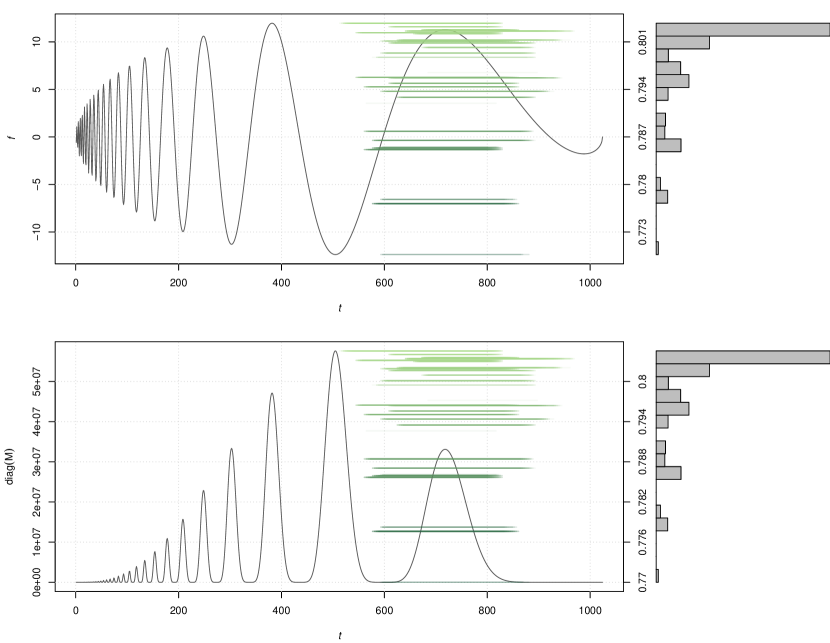
Figure 6: Top 2% of $B$ for the ‘Doppler’ time series and secondary function $\mathbf{g}_{4}$ in Example 3.4. Each horizontal line segment represents an interval $B$, and the height of each segment is proportional to the improvement over the approximation which ignores secondary analysis, $\tilde{\boldsymbol{f}}$. The ratio of squared error loss for $\hat{\boldsymbol{f}}_{B}$ to that of $\tilde{\boldsymbol{f}}$ is shown in the right axis. The histogram to the right of each plot shows the distribution of the top 2% of proposed intervals. Some segments $B$ have the same relSE, so the histogram helps to illuminate where segments have overlapped.

4 Discussion and Future Work

There are many hurdles to clear in DOE’s race towards exascale high performance computing environments including future system architectures, power/energy compliance, and many others. In this paper, we discuss one such problem related to the overwhelming demands being placed on I/O and storage systems due to the increased volume of data being generated by computational experiments. We remind the reader that our treatment of this larger-scale problem is in no way complete. However, we do believe that our codification of a simpler class of heterogeneous wavelet-based compression strategies will provide practitioners and theoreticians a systematic framework for future work. Our initial experiments given in Section 3 certainly supports this assertion.

In closing, we will briefly discuss the obvious extension for this current work. First, it may be unrealistic to assume that we know an importance function a priori. Consider our motivating example involving wind turbine arrays. We might know the approximate locations within the simulation domain that we would like to store in a high fidelity, however, the precise locations will be unknown at run-time. In other words, we will need to estimate the optimal prioritized region without using $\mathbf{g}(\boldsymbol{f})$ and an exhaustive (or near-exhaustive) search. A smart in situ sampling strategy of the data should enable the development of a reasonably good estimator, $\hat{\mathbf{M}}$.

Acknowledgements

The authors would like to thank Professor Jay Breidt and David Biagioni for their suggestions on improving early drafts of this manuscript.

This work was supported by the Laboratory Directed Research and Development (LDRD) Program at the National Renewable Energy Laboratory. NREL is a national laboratory of the U.S. Department of Energy Office of Energy Efficiency and Renewable Energy operated by the Alliance for Sustainable Energy, LLC.

Appendix A Nearly Exhaustive Searches

All data used in the examples in this paper were of size 1024. When searching for the optimal $B$, we were unable to consider every interval within $T$, however we we able to consider nearly every interval, and we do not expect substantive changes would occur in our results if we did check all possibilities.

By nearly exhaustive, we mean the following. Instead of all intervals

$$\{a,\dots,b\},\quad 1\leq a<b\leq n,$$

we considered only intervals of the form where

$$a =4x+1,\quad x=1,\dots,255$$

$$b =4y+a, \text{for all }y=1,\dots,81\text{ such that }b<1024.$$

We therefore considered all intervals of length equal to a multiple of 4 up to 324, and left boundary equal to all integers with a value of 1 modulo 4 up to 1021, e.g., we checked $513\dots 513+32$ but not $514\dots 514+32$. For the cases where this system led to ranges that would extend beyond $\{1,\dots,1024\}$, we simply took the intersection of the proposed $B$ with $T$. The convenience of this systematic approach outweighed the slight preference shown for boundaries that included points near the right edge of $\{1,\dots,1024\}$

This nearly-exhaustive method was used for convenience. The computational demands for implementation were reasonable for a personal laptop computer (on the order of 10 minutes per search).

References

- Ahern et al., [2011] Ahern, S., Shoshani, A., Ma, K.-L., Choudhary, A., Critchlow, T., Klasky, S., Pascucci, V., Ahrens, J., Bethel, E., Childs, H., et al. (2011). Scientific discovery at the exascale. report from the doe ascr 2011 workshop on exascale data management. Analysis, and Visualization.
- Ashby et al., [2010] Ashby, S., Beckman, P., Chen, J., Colella, P., Collins, B., Crawford, D., Dongarra, J., Kothe, D., Lusk, R., Messina, P., et al. (2010). The opportunities and challenges of exascale computing. Summary Report of the Advanced Scientific Computing Advisory Committee (ASCAC) Subcommittee (November 2010).
- Casella and Berger, [2002] Casella, G. and Berger, R. L. (2002). Statistical inference. Duxbury/Thomson Learning.
- Chandler and Hemami, [2005] Chandler, D. M. and Hemami, S. S. (2005). Dynamic contrast-based quantization for lossy wavelet image compression. Image Processing, IEEE Transactions on, 14(4):397–410.
- Chen et al., [2013] Chen, J., Choudhary, A., Feldman, S., Hendrickson, B., Johnson, C., Mount, R., Sarkar, V., White, V., and Williams, D. (2013). Synergistic challenges in data-intensive science and exascale computing. DOE ASCAC Data Subcommittee Report, Department of Energy Office of Science.
- Clyne et al., [2010] Clyne, J., Gruchalla, K., and Rast, M. (2010). Vapor: Visual, statistical, and structural analysis of astrophysical flows. In Numerical Modeling of Space Plasma Flows, Astronum-2009, volume 429, page 323.
- Donoho and Johnstone, [1995] Donoho, D. L. and Johnstone, I. M. (1995). Adapting to unknown smoothness via wavelet shrinkage. Journal of the american statistical association, 90(432):1200–1224.
- Donoho and Johnstone, [1994] Donoho, D. L. and Johnstone, J. M. (1994). Ideal spatial adaptation by wavelet shrinkage. Biometrika, 81(3):425–455.
- Gruchalla, [2009] Gruchalla, K. (2009). Progressive Visualization-Driven Multivariate Feature Definition and Analysis. PhD dissertation, University of Colorado at Boulder.
- Gruchalla et al., [2009] Gruchalla, K., Rast, M., Bradley, E., Clyne, J., and Mininni, P. (2009). Visualization-driven structural and statistical analysis of turbulent flows. In Advances in Intelligent Data Analysis VIII, pages 321–332. Springer.
- Gruchalla et al., [2011] Gruchalla, K., Rast, M., Bradley, E., and Mininni, P. (2011). Segmentation and visualization of multivariate features using feature-local distributions. In Advances in Visual Computing, pages 619–628. Springer.
- Hilton, [1997] Hilton, M. L. (1997). Wavelet and wavelet packet compression of electrocardiograms. Biomedical Engineering, IEEE Transactions on, 44(5):394–402.
- Nayson, [2008] Nayson, G. P. (2008). Wavelets Methods in Statistics with R. Springer, first edition.
- Skodras et al., [2001] Skodras, A., Christopoulos, C., and Ebrahimi, T. (2001). The JPEG 2000 still image compression standard. Signal Processing Magazine, IEEE, 18(5):36–58.