A deep narrowband imaging search for C IV and He II emission from Ly$\alpha$ Blobs

Abstract

We conduct a deep narrow-band imaging survey of 13 Ly$\alpha$ blobs (LABs) located in the SSA22 proto-cluster at $z\sim 3.1$ in the C IV and He II emission lines in an effort to constrain the physical process powering the Ly$\alpha$ emission in LABs. Our observations probe down to unprecedented surface brightness limits of 2.1 – 3.4 $\times$ $10^{-18}$ erg s^-1 cm^-2 arcsec^-2 per 1 arcsec² aperture (5$\sigma$) for the He II $\lambda$1640 and C IV $\lambda$1549 lines, respectively. We do not detect extended He II and C IV emission in any of the LABs, placing strong upper limits on the He II/Ly$\alpha$ and C IV/Ly$\alpha$ line ratios, of 0.11 and 0.16, for the brightest two LABs in the field. We conduct detailed photoionization modeling of the expected line ratios and find that, although our data constitute the deepest ever observations of these lines, they are still not deep enough to rule out a scenario where the Ly$\alpha$ emission is powered by the ionizing luminosity of an obscured AGN. Our models can accommodate He II/Ly$\alpha$ and C IV/Ly$\alpha$ ratios as low as $\simeq 0.05$ and $\simeq 0.07$ respectively, implying that one needs to reach surface brightness as low as 1 – 1.5 $\times$ $10^{-18}$ erg s^-1 cm^-2 arcsec^-2 (at 5$\sigma$) in order to rule out a photoionization scenario. These depths will be achievable with the new generation of image-slicing integral field units such as VLT/MUSE or Keck/KCWI. We also model the expected He II/Ly$\alpha$ and C IV/Ly$\alpha$ in a different scenario, where Ly$\alpha$ emission is powered by shocks generated in a large-scale superwind, but find that our observational constraints can only be met for shock velocities $v_{\rm s}\gtrsim$ 250 km s^-1, which appear to be in conflict with recent observations of quiescent kinematics in LABs.

1. Introduction

In the current $\Lambda$CDM paradigm of structure formation, gas collapses onto the potential wells of dark matter halos, and whether it shock heats to the halo virial temperature and cools slowly, or flows in preferentially along cold filamentary streams (Dekel et al. 2009), its gravitational energy is eventually radiated away, as it settles into galactic disks and forms stars. This star formation results in the growth of galactic bulges, and in the innermost regions, the gas could also accrete onto a supermassive black hole powering an active galactic nucleus (AGN). Many have theorized (e.g., Silk & Rees 1998; Fabian 1999; King 2003) that star-formation and/or BH accretion could be self-regulating, such that “feedback” processes inject energy back into the inter-stellar medium (ISM), heating the gas, and preventing further star-formation or accretion.

The complex interplay of gas accreted from the intergalactic medium (IGM) and the galactic outflows which may be the signatures of mechanical/radiative feedback are poorly understood, particularly at high-redshift, where the feedback processes are often invoked as being most intense. These processes conspire to determine the structure of the circumgalactic medium (CGM), which comprises the interface between galaxies and the IGM. At high redshift, the CGM has been extensively studied by analyzing absorption features in the spectra of background sources. A significant amount of effort has been devoted to the studying of the CGM of the so-called Lyman break galaxies (LBGs), star-forming galaxies at $z\sim 2$ (Adelberger et al. 2005; Steidel et al. 2010; Crighton et al. 2011; Rakic et al. 2012; Rudie et al. 2012; Crighton et al. 2013, 2014). These studies have illustrated that typical star-forming galaxies exhibit a modest $\sim 20\%$ covering factor of optically thick neutral hydrogen (Rudie et al. 2012), and enrichment levels ranging from extremely metal-poor (Crighton et al. 2013) to nearly solar (Crighton et al. 2014). On the other hand, using projected QSO pairs, Hennawi et al. (2006) launched an innovative technique to study the properties of the gas on scales of a few 10 kpc to several Mpc of the much more massive dark matter halos traced by quasars, initiating the Quasars Probing Quasars survey (Hennawi & Prochaska 2007; Prochaska & Hennawi 2009; Hennawi & Prochaska 2013; Prochaska et al. 2013a, b). These studies have revealed a massive $(\gtrsim 10^{10}$ M_⊙) resevoir of cool ($T\simeq 10^{4}\,{\rm K}$ gas in the CGM of massive halos (see also Bowen et al. 2006; Farina et al. 2013), which appears to be in conflict with the predictions of hydrodynamical zoom-in simulations of galaxy formation (Fumagalli et al. 2014).

These absorption studies are however, limited by the paucity of bright background sources, and by the inherently one-dimensional nature of the technique. Complementary information can be obtained by directly observing the CGM in emission, and this emission may be easier to detect in AGN environments. In particular, if an AGN illuminates the cool CGM gas around it, the reprocessed emission (fluorescence) from this cool medium could be detectable as extended Ly$\alpha$ emission (e.g., Rees 1988; Haiman & Rees 2001). Indeed, many searches for emission from the CGM of QSOs have been undertaken, reporting detections on scale of $10-50$ kpc around $z\sim 2-4$ QSOs (e.g, Hu & Cowie 1987; Heckman et al. 1991a, b; Christensen et al. 2006; North et al. 2012). Recently Cantalupo et al. (2014) reported the discovery of an extraordinary extended ($\sim 500$ kpc) Ly$\alpha$ nebula around the radio-quiet QSO UM287, believed to be fluorescent emission powered by the QSO radiation. This discovery is part of a large homogenous survey of emission from the CGM of quasars which will enable statistical studies of this phenomenon (e.g., Arrigoni Battaia et al. 2014).

Extended Ly$\alpha$ nebulae have also been frequently observed also around high-redshift ($z\geq 2$) radio galaxies (HzRGs; e.g., McCarthy 1993; van Ojik et al. 1997; Nesvadba et al. 2006; Villar-Martín et al. 2007; Reuland et al. 2007). With an avarage Ly$\alpha$ luminosity of $L_{{\rm Ly}\alpha}\sim 10^{44.5}$ erg s^-1 and a diameter $\gtrsim 100$ kpc, these nebulae tend to be brighter and larger than those around QSOs, although current surveys are very inhomogenous. But an important difference between these two types of nebulae is that for quasars a strong source of ionizing photons is directly identified, whereas for the HzRGs this AGN is obscured from our perspective (see e.g. Miley & De Breuck, 2008)), in accord with unified models of AGN (e.g., Antonucci 1993; Urry & Padovani 1995; Elvis 2000). Further, the study of the properties of the gas surrounding HzRGs has to take into account the impact of the complicated interaction between the strong radio jets and the ambient gas.

Intriguingly, the so-called Ly$\alpha$ blobs (LABs), large (50–100 kpc) luminous ($L$(Ly$\alpha$) $\sim$ 10^43-44 erg s^-1) Ly$\alpha$ nebulae at $z\sim 2-6$, exhibit properties similar to Ly$\alpha$ nebulae around QSOs and HzRGs, but without obvious evidence for the presence of an AGN (e.g., Keel et al., 1999; Steidel et al., 2000; Francis et al., 2001; Matsuda et al., 2004, 2011; Dey et al., 2005; Saito et al., 2006; Smith & Jarvis, 2007; Ouchi et al., 2009; Prescott et al., 2009, 2012; Yang et al., 2009, 2010). LABs are believed to be the sites of massive galaxy formation, where strong feedback processes may be expected to occur (Yang et al. 2010). However, despite intense interest and multi-wavelength studies, the physical mechanism powering the Ly$\alpha$ emission in the LABs is still poorly understood. The proposed scenarios include photo-ionization by AGNs (Geach et al., 2009), shock-heated gas by galactic superwinds (Taniguchi & Shioya, 2000), cooling radiation from cold-mode accretion (Fardal et al., 2001; Haiman et al., 2000; Dijkstra & Loeb, 2009; Goerdt et al., 2010; Faucher-Giguère et al., 2010), and resonant scattering of Ly$\alpha$ from star-forming galaxies (Steidel et al., 2011; Hayes et al., 2011).

Our ignorance of the physical process powering the emission in LABs likely results from the current lack of other emission-line diagnostics besides the strong Ly$\alpha$ line (e.g., Matsuda et al., 2006). In this paper, we attempt to remedy this problem, by searching for emission in two additional rest-frame UV lines, namely C IV $\lambda$1549 and He II $\lambda$1640. We present deep narrowband imaging observations tuned to the C IV $\lambda$1549 and He II $\lambda$1640 emission lines of 13 LABs at $z\sim 3.1$ in the well-known SSA22 proto-cluster field (Steidel et al. 2000; Hayashino et al. 2004; Matsuda et al. 2004). Our observations exploit a fortuitous match between two narrowband filters on VLT/FORS2 and the wavelengths of the redshifted CIV and HeII emission lines of a dramatic overdensity of LABs (and Ly$\alpha$ emitters (LAEs)) in the SSA22 field (Matsuda et al. 2004; Figure 1), and achieve unprecedented depth. This overdensity results in a large multiplexing factor allowing us to carry out a sensitive census of C IV/Ly$\alpha$ and He II/Ly$\alpha$ line ratios for a statistical sample of LABs in a single pointing.

In the following, we review four mechanisms which have been proposed to power the Ly$\alpha$ blobs, which could also possibly act together, and discuss how they might generate C IV and He II line emission.

1. Photoionization by a central AGN: as stressed above, it is well established that the ionizing radiation from a central AGN can power giant Ly$\alpha$ nebulae, with sizes up to $\sim$200 kpc, around high-$z$ radio galaxies (e.g., Villar-Martín et al. 2003b; Reuland et al. 2003; Venemans et al. 2007) and quasars (e.g., Heckman et al. 1991b; Christensen et al. 2006; Smith et al. 2009; Cantalupo et al. 2014). If the halo gas is already polluted with heavier elements (e.g., C, O) by outflows from the central source, one expects to detect both C IV and He II emission from the extended Ly$\alpha$-emitting gas. If not, only extended He II emission is expected. Indeed, extended C IV and He II emission have been clearly detected in HzRGs (Villar-Martín et al. 2003a; Humphrey et al. 2006; Villar-Martín et al. 2007) and tentatively detected around QSOs (Heckman et al. 1991b, a; Humphrey et al. 2013) on scales of 10-100 kpc. The photoionization scenario gains credence from a number of studies suggesting that LABs host an AGN which is obscured from our perspective (Geach et al. 2009; Overzier et al. 2013; Yang et al. 2014a, but see Nilsson et al. 2006; Smith & Jarvis 2007).

2. Shocks powered by galactic-scale outflows: Several studies have argued that shell-like or filamentary morphologies, large Ly$\alpha$ line widths ($\sim$1000 km s^-1), and enormous Ly$\alpha$ sizes ($\sim$100 kpc) imply that extreme galactic-scale outflows, and specifically the ionizing photons produced by strong shocks, power the LABs (Taniguchi & Shioya, 2000; Taniguchi et al., 2001; Ohyama et al., 2003; Wilman et al., 2005; Mori & Umemura, 2006). If violent star-formation feedback powers a large-scale superwind, the halo should be highly enriched, and with a significant amount of gas at $T\sim 10^{5}\,{\rm K}$. One would therefore also expect to detect extended He II and C IV emission, but with potentially different line ratios than the simple photoionization case. Note that collisional excitations of singly ionized helium peaks at $T\sim 10^{5}\,{\rm K}$, making the He II line one of the dominant observable coolants at this temperature (Yang et al. 2006). Note however, that the relatively quiescent ISM kinematics of star-forming galaxies embedded within LABs appear to be at odds with this scenario (McLinden et al. 2013; Yang et al. 2011, 2014b).

3. Gravitational cooling radiation: A large body of theoretical work has suggested that Ly$\alpha$ emission nebulae could result from Ly$\alpha$ cooling radiation powered by gravitational collapse (Haiman et al., 2000; Furlanetto et al., 2005; Dijkstra et al., 2006; Faucher-Giguère et al., 2010; Rosdahl & Blaizot, 2012). In the absence of significant metal-enrichment, collisionally excited Ly$\alpha$ is the primary coolant of $T\sim 10^{4}\,{\rm K}$ gas; hence cool gas steadily accreting onto halos hosting Ly$\alpha$ blobs may radiate away their gravitational potential energy in the Ly$\alpha$ line. However, the predictions of the Ly$\alpha$ emission from these studies are uncertain by orders of magnitude (e.g. Furlanetto et al., 2005; Faucher-Giguère et al., 2010; Rosdahl & Blaizot, 2012) because the emissivity of collisionally excited Ly$\alpha$ is exponentially sensitive to gas temperature. Accurate prediction of the temperature requires solving a coupled radiative transfer and hydrodynamics problem which is not currently computational feasible (but see Rosdahl & Blaizot, 2012). While Yang et al. (2006) suggest that the He II cooling emission could be as high as 10$\%$ of Ly$\alpha$ near the embedded galaxies (i.e. point-source emission) where the density of IGM/CGM is highest, the extended ($\gtrsim 20$ kpc) He II emission may be challenging to detect with current facilities (${\rm HeII/Ly\alpha}<0.1$). Note that if Ly$\alpha$ emission arises from cooling radiation of pristine gas, no extended C IV emission is expected.

4. Resonant scattering of Ly$\alpha$ from embedded sources: In this scenario, Ly$\alpha$ photons are produced in star-forming galaxies or AGNs embedded in the LABs, but the extended sizes of the Ly$\alpha$ halos result from resonant scattering of Ly$\alpha$ photons as they propagate outwards (Dijkstra & Loeb, 2008; Hayes et al., 2011; Cen & Zheng, 2013; Cantalupo et al., 2014). In this picture, non-resonant He II emission (if produced in the galaxies or AGN) should be compact, in contrast with the extended Ly$\alpha$ halos. In other words, if extended He II is detected on the same scale as the extended Ly$\alpha$ emission, this implies that resonant scattering does not play a significant role in determining the extent of the Ly$\alpha$ nebulae. Conversely, as the C IV line is a resonant line, it is conceivable that extended emission could arise due to scattering by the same medium scattering Ly$\alpha$, provided that the halo gas is optically thick to C IV, which in turn depends on the metallicity and ionization state of the halo gas. In this context, it is interesting to note that Prochaska et al. (2014) find a high covering factor of optically thick C II and C IV absorption line systems out to $>200$ kpc around $z\sim 2$ QSOs, implying that the CGM of massive halos is significantly enriched.

In summary, a detection of extended emission in the C IV line will provide us information on the intensity and hardness of an ionizing source or the speed of shocks in a superwind (e.g., Ferland et al., 1984; Nagao et al., 2006; Allen et al., 2008), the metallicity of gas in the CGM of LABs, and the sizes of metal-enriched halos. A detection of extended (non-resonant) He II emission similarly constrains the ionizing spectrum or the speed of shocks, and can be used to test whether Ly$\alpha$ photons are resonantly scattered, as well as constrain the amount of material in a warm $T\sim 10^{5}\,{\rm K}$ phase. To date, there are five detections of extended C IV and He II emission from LABs reported in the literature (Dey et al. 2005 and Prescott et al. 2009, 2013). The extended C IV and He II emission from these Ly$\alpha$ nebulae has fluxes up to $F_{\rm CIV}\sim 4\times 10^{-17}$ erg s^-1 cm^-2 and $F_{\rm HeII}\sim 6\times 10^{-17}$ erg s^-1 cm^-2, implying C IV/Ly$\alpha$ $\lesssim 0.13$ and He II/Ly$\alpha$ $\lesssim 0.13$. Publication bias, i.e. the fact that searches for these lines that resulted in non-detections are likely to have gone unpublished, makes it challenging to assess rate of detections in LABs, which is one of the goals of the present work.

This paper is organized as follows. In §2, we describe our VLT/FORS2 narrowband imaging observations, the data reduction procedures, and the surface brightness limits of our images. In §3, we present our measurements for C IV and He II lines. §4 describes previous measurements for C IV and He II in the literature. In §5, we discuss photoionization models and shock models for LABs, and compare them with our observations and other sources in the literature. §6 summarizes our conclusions. Throughout this paper, we adopt the cosmological parameters $H_{0}=70$ km s^-1 Mpc^-1, $\Omega_{M}=0.3$ and $\Omega_{\Lambda}=0.7$. In this cosmology, 1″ corresponds to 7.6 physical kpc at $z=3.1$. All magnitudes are in the AB system (Oke 1974).

2. Observations and data reduction

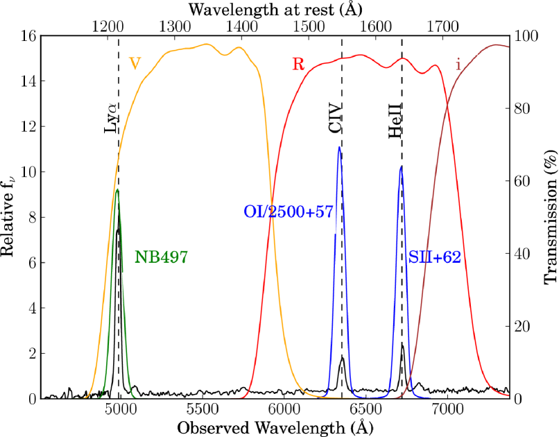
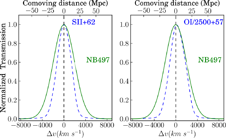
Figure 1.— Top panel: Filter response profiles for the narrowband filters NB497 (green), SII+62 and OI/2500+57 (blue) and the broad-band filters $V$ (orange), $R$ (red) and $i$ (brown) overplotted on a composite radio galaxy spectrum (McCarthy 1993). Bottom panels: Comparison between the NB497 (green) and the SII+62 and OI/2500+57 (dashed blue) filters shifted to match the narrowband filter used for Ly$\alpha$ (Matsuda et al., 2004). The filter curves are here normalized to their peak value and plotted with respect to the velocity and comoving distance probed. Note the nearly perfect match between the Ly$\alpha$ narrowband filter and the two FORS2 narrowband filters used for C IV $\lambda$1549 and He II $\lambda$1640 in this work.

2.1. VLT/FORS2 observations and data reduction

We obtained deep C IV and He II narrowband images of 13 LABs in the SSA22 proto-cluster field, including the two largest LABs that were originally discovered by Steidel et al. (2000). Data were taken in service-mode using the FORS2 instrument on the VLT 8.2m telescope Antu (UT1) on 2010 August, September, October and 2011 September over 25 nights. We used two narrowband filters, OI/2500+57 and SII+62 matching the redshifted C IV $\lambda$1549 and He II $\lambda$1640 at $z=3.1$, respectively. The OI/2500+57 filter has a central wavelength of $\lambda_{c}\approx 6354$ Å and has a FWHM of $\Delta\lambda_{\rm FWHM}\approx 59$ Å, while the SII+62 filter has $\lambda_{c}\approx 6714$ Å and $\Delta\lambda_{\rm FWHM}\approx 69$ Å (Fig. 1). The FORS2 has a pixel scale of 0$\farcs$25 pixel^-1 and a field of view (FOV) of 7′$\times$7′ that allow us to observe a total of 13 LABs in a single pointing. The pointing was chosen to maximize the number of Ly$\alpha$ blobs while including the two brightest LABs, LAB1 and LAB2 (Steidel et al. 2000). We show the spatial distribution of $\sim$300 LAEs and 35 LABs in the SSA22 region and mark the LABs within FORS2 narrowband images in Figure 2.

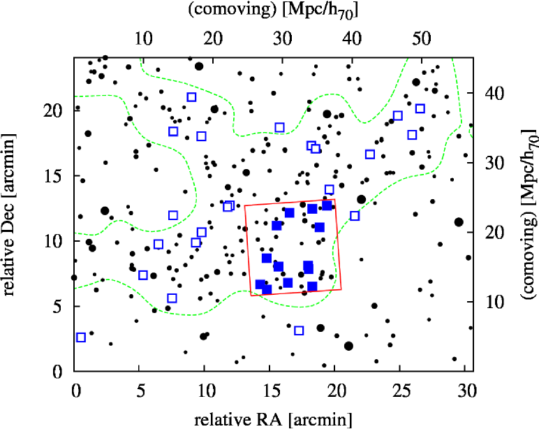
Figure 2.— Spatial distribution of the Ly$\alpha$ emitters (black filled circles) and Ly$\alpha$ blobs (blue squares) in the SSA22 proto-cluster (Hayashino et al., 2004; Matsuda et al., 2004). The red box is the FOV of our FORS2 imaging (7′$\times$ 7′) which includes 13 LABs (blue filled squares). The green dashed line indicates high-density region traced by the Ly$\alpha$ emitters.

The total exposure time was 19.9 and 19.0 hours for C IV and He II lines, respectively. These exposures consist of 71 and 68 individual exposures of $\sim$17 minutes, taken with a dither pattern to fill in a gap between the two chips, and to facilitate the removal of cosmic rays. Because our targets are extended over 5″–17″ diameter and our primary goal is to detect the extended features rather than compact embedded galaxies, we carried out our observations under any seeing conditions (program ID: 085.A-0989, 087.A-0297). Figure 3 shows the distribution of FWHMs measured from stars in individual exposures. Although the observations were carried out under poor or variable seeing condition, the seeing ranges from 0$\farcs$5 to 1$\farcs$4 depending on the nights and the median seeing is $\sim$0$\farcs$8 in both filters. In Table 1, we summarize our VLT/FORS2 narrowband observations.

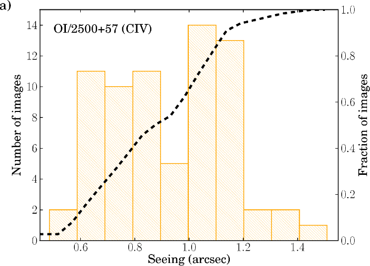
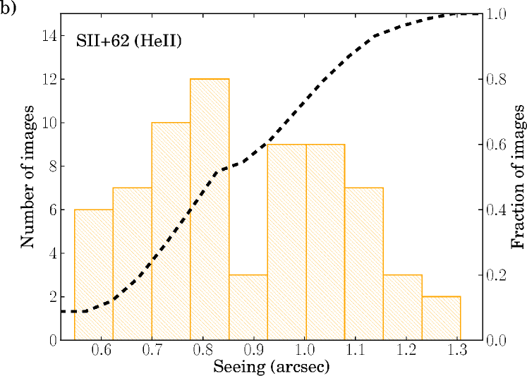
Figure 3.— (a) Distribution of seeings for the OI/2500+57 (C IV $\lambda$1549) images. (b) Same for the SII+62 (He II $\lambda$1640) images. The black dashed lines indicate the cumulative distribution. The median seeing is $\sim$0$\farcs$8 for both C IV and He II images.

The data were reduced with standard routines using IRAF. The images were bias-subtracted and flat-fielded using twilight flats. To improve the flat-fielding essential for detecting faint extended emission across the fields, we further correct for the illumination patterns using night-sky flats. The night-sky flats were produced by combining the unregistered science frames with an average sigma-clipping algorithm after masking out all the objects. Satellite trails, CCD edges, bad pixels, and saturated pixels are masked. Each individual frame is cleaned from cosmic rays using the L.A.Cosmic algorithm (van Dokkum 2001). The astrometry was calibrated with the SDSS-DR7 $r$-band catalogue using SExtractor and SCAMP (Bertin 2006). The RMS uncertainties in our astrometric calibration are $\sim$0$\farcs$2 for both C IV and He II images.

The final stacks for each filter (C IV and He II) were obtained using SWarp (Bertin et al. 2002): the individual frames were sky-subtracted using a background mesh size of 256 pixels ($\approx 64$″), then projected onto a common WCS using a Lanczos3 interpolation kernel, and average-combined with weights proportional to flat and night-sky flat images. Note that we choose the mesh size to be large enough to ensure that we do not mistakenly subtract any extended emission as sky background. For flux calibration, we use four spectrophotometric standard stars (Feige110, EG274, LDS749B, and G158-100) that were repeatedly observed during our observations. Typical uncertainties in the derived zero-points are $\approx$0.03 mag.

2.2. Subaru Suprime-Cam Data

To subtract continuum from our narrowband images and compare the C IV and He II line fluxes with those of Ly$\alpha$, we rely on previous Subaru observations. The SSA22 field has been extensively observed in $B$, $V$, $R$, $i^{\prime}$, and NB497 bands (Hayashino et al. 2004, Matsuda et al. 2004) with the Subaru Suprime-Cam (Miyazaki et al. 2002). These images have a pixel scale of 0$\farcs$20 and a FOV of 34′$\times$ 27′. The NB497 narrowband filter, tuned to Ly$\alpha$ line at $z$ $\sim$ 3.1, has a central wavelength of 4977 Å and a FWHM of 77 Å. The total exposure time for the Ly$\alpha$ narrowband image was 7.2 hours with a $5\sigma$ sensitivity of $5.5\times 10^{-18}$ erg s^-1 cm^-2 arcsec^-2 per 1 arcsec² aperture, which is roughly 1.5 – 2.5 times shallower than those of FORS2 He II and C IV images. In Table 1, we summarize the Subaru broadband and narrowband images that were used in this work.

Table 1VLT FORS2 Observations and Subaru Data

Telescope	Instrument	Filter (target line)	$\lambda_{\rm Central}^{a}$	$\Delta\lambda_{\rm FWHM}^{b}$	Seeingc	Exp. Time	Depthd	Pixel Scale
			(Å)	(Å)	(arcsec)	(hours)	(mag)	(arcsec)
VLT	FORS2	OI/2500+57 (CIV)	6354	59	0.8	19.9	25.9	0.25
VLT	FORS2	SII+62 (HeII)	6714	69	0.8	19.0	26.5	0.25
Subarue	S-Cam	NB497 (Ly$\alpha$)	4977	77	1.0	7.2	26.2	0.20
Subarue	S-Cam	$R$	6460	1177	1.0	2.9	26.7	0.20

Using these deep Subaru data, Matsuda et al. (2004) found 35 LABs, defined to be Ly$\alpha$ emitters with the observed EW(Ly$\alpha$) $>$ 80 Å and an isophotal area larger than 16 arcsec², which corresponds to a spatial extent of 30 kpc at $z=3$. The isophotal area was measured above the $2\sigma$ surface brightness limit ($2.2\times 10^{-18}$ erg s^-1 cm^-2 arcsec^-2). In Table 2, we list the properties (e.g., Ly$\alpha$ luminosity and isophotal area) of the 13 LABs that were observed with VLT/FORS2. We refer readers to Matsuda et al. (2004) for more details of this Ly$\alpha$ blob sample.

Table 2Properties of the 13 LABs in our sample.

Object	$F$(Ly$\alpha$)	$L$(Ly$\alpha$)	Area	SB (Ly$\alpha$)	SB (CIV)	SB (HeII)	CIV/Ly$\alpha$	HeII/Ly$\alpha$
	(1)	(2)	(3)	(4)	(5)	(6)	(7)	(8)
LAB1	9.4	7.8	200	4.7	$<$0.74	$<$0.50	$<$0.16	$<$0.11
LAB2	8.2	6.8	145	5.6	$<$0.89	$<$0.63	$<$0.16	$<$0.11
LAB7	1.3	1.1	36	3.6	$<$1.19	$<$0.99	$<$0.33	$<$0.27
LAB8	1.5	1.3	36	4.2	$<$1.24	$<$0.93	$<$0.29	$<$0.22
LAB11	0.8	0.6	28	2.8	$<$1.23	$<$1.08	$<$0.44	$<$0.38
LAB12	0.7	0.6	27	2.7	$<$1.29	$<$1.06	$<$0.48	$<$0.39
LAB14	1.1	0.9	25	4.5	$<$1.38	$<$1.10	$<$0.31	$<$0.24
LAB16	1.0	0.9	25	4.1	$<$1.39	$<$1.07	$<$0.34	$<$0.26
LAB20	0.6	0.5	22	2.8	$<$1.35	$<$1.16	$<$0.48	$<$0.41
LAB25	0.6	0.5	22	2.7	$<$1.36	$<$1.12	$<$0.50	$<$0.41
LAB30	0.9	0.8	17	5.8	$<$1.45	$<$1.36	$<$0.25	$<$0.23
LAB31	1.2	1.0	19	6.6	$<$1.44	$<$1.18	$<$0.22	$<$0.18
LAB35	1.0	0.8	17	5.9	$<$1.52	$<$1.29	$<$0.26	$<$0.22

Note. — (1) Ly$\alpha$ line flux within the isophote in $10^{-16}$ erg s^-1 cm^-2, (2) Ly$\alpha$ luminosity in 10⁴³ erg s^-1, (3) isophotal area in arcsec² above $2.2\times 10^{-18}$ erg s^-1 cm^-2 arcsec^-2, (4) average surface brightness within the isophote, (5) 5$\sigma$ upper limits on C IV surface brightness, (6) 5$\sigma$ upper limits on He II surface brightness, (7–8) 5$\sigma$ upper limits C IV/Ly$\alpha$ and He II/Ly$\alpha$ line ratios. All surface brighnesses are given in unit of 10^-18 erg s^-1 cm^-2 arcsec^-2.

2.3. Continuum subtraction

To identify the emission in the C IV $\lambda$1549 and He II $\lambda$1640 lines we subtract the continuum emission underlying the OI/2500+57 and SII+62 filter. We estimate the continuum using the deep Subaru $R$ band image. Because the Subaru and FORS2 images have different pixel scales, we resample the $R$-band image to the FORS2 pixel scale and register them to our WCS in order to compare all the images pixel by pixel. We do not match the point spread functions (PSFs) given that FORS2 images were obtained with a wide range of seeing and we are mostly interested in the extended emission. We produce the continuum subtracted image for each filter (C IV and He II) using the following relations (Yang et al. 2009):

$$f_{\lambda,\,{\rm cont}}^{B\!B}=\frac{F_{B\!B}-F_{N\!B}}{\Delta\lambda_{B\!B}-\Delta\lambda_{N\!B}}$$ (1)

$$F_{\rm line}=F_{N\!B}-f_{\lambda,\,{\rm cont}}^{B\!B}\Delta\lambda_{N\!B},$$ (2)

where $F_{B\!B}$ is the flux in the $R$ band, $F_{N\!B}$ is the flux in one of the narrowband filters. $\Delta\lambda_{B\!B}$ and $\Delta\lambda_{N\!B}$ represent the FWHM of the $R$ and narrowband filters, respectively. $f_{\lambda,\,{\rm cont}}^{B\!B}$ is the flux density of the continuum within the $R$ band, and $F_{\rm line}$ is the line flux (C IV or He II).

2.4. Surface Brightness Limits

We compute a global surface brightness limit for detecting He II and C IV lines using a global root-mean-square (rms) of the images. To calculate the global rms per pixel, we first mask out the sources, in particular the scattered light and halos of bright foreground stars, and compute the standard deviation of sky regions using a sigma-clipping algorithm. We convert these rms values into the surface brightness (SB) limits per 1 sq. arcsec aperture. We find that the 1$\sigma$ detection limit per 1 arcsec² aperture (${\rm SB}_{1}$) is $4.2\times 10^{-19}$ and $6.8\times 10^{-19}$ erg s^-1 cm^-2 arcsec^-2 for He II and C IV, respectively. These represent the deepest He II $\lambda$1640 and C IV $\lambda$1549 narrow-band images ever taken.

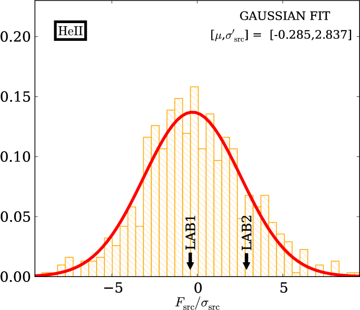
Figure 4.— Analysis of the systematics in the He II line image. Left: Distribution of the normalized flux, $F_{\rm src}$/$\sigma_{\rm src}$ for random circular apertures with the same extent as LAB1 and LAB2. Here, $F_{\rm src}$ is a total flux within an aperture and $\sigma_{\rm src}$ is the expected 1$\sigma$ flux limit in an ideal case with uniform noise properties, i.e., $\sigma_{\rm src}$ = ${\rm SB}_{1}\sqrt{A_{\rm src}}$. The Gaussian fit to the histogram is highlighted in red. The observed values for LAB1 and LAB2 are shown by the black arrows. Right: Same for all the other LABs with $A_{\rm src}$ $<$ 40 arcsec² in our sample. The black arrows indicate the value of each LAB. Note that in the absence of systematics, i.e., in ideal conditions when the sky and continuum subtractions are perfect, these histograms should be a Gaussian with unit variance, but they are $\approx 3$ or $\approx 2$ times broader, i.e., $\sigma^{\prime}_{\rm src}$ $\approx$ 2–3 $\sigma_{\rm src}$.

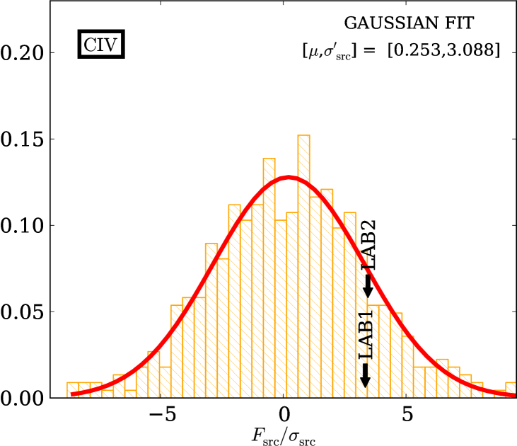
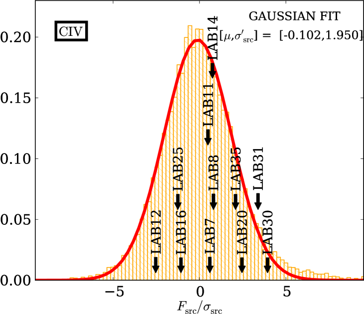
Figure 5.— Analysis of the systematics in the C IV line image. Left: Distribution of the normalized flux, $F_{\rm src}$/$\sigma_{\rm src}$ for random circular apertures with the same extent as LAB1 and LAB2. Here, $F_{\rm src}$ is a total flux within an aperture and $\sigma_{\rm src}$ is the expected 1$\sigma$ flux limit in an ideal case with uniform noise properties, i.e., $\sigma_{\rm src}$ = ${\rm SB}_{1}\sqrt{A_{\rm src}}$. The Gaussian fit to the histogram is highlighted in red. The observed values for LAB1 and LAB2 are shown by the black arrows. Right: Same for all the other LABs with $A_{\rm src}$ $<$ 40 arcsec² in our sample. The black arrows indicate the value of each LAB. Note that in the absence of systematics, i.e., in ideal conditions when the sky and continuum subtractions are perfect, these histograms should be a Gaussian with unit variance, but they are $\approx 3$ or $\approx 2$ times broader, i.e., $\sigma^{\prime}_{\rm src}$ $\approx$ 2–3 $\sigma_{\rm src}$.

The sensitivity required to detect an extended source depends on its size because one can reach lower surface brightness levels by spatially averaging. In an ideal case of perfect sky and continuum subtraction, the 1$\sigma$ SB limit for an extended source is given by ${\rm SB}_{1}$/$\sqrt{A_{\rm src}}$, where $A_{\rm src}$ is the isophotal area in arcsec² and ${\rm SB}_{1}$ is the surface brightness limit per 1 arcsec² aperture. However, in practice the actual detection limits are limited by systematics resulting from imperfect sky and continuum subtraction. Therefore, we empirically determine the detection limits for extended sources with different sizes as follows.

In the continuum-subtracted line images, we mask all the artifacts (e.g., CCD edges and scattered light from bright stars) and also the locations of the LABs. For each LAB that we consider, we randomly place circular apertures with the same area of the LAB and extract the fluxes ($F_{\rm src}$) within these apertures. If the images have uniform noise properties in the absence of systematics, the fluxes ($F_{\rm src}$) from many random apertures should follow a Gaussian distribution with a width of $\sigma_{\rm src}$ $\equiv$ ${\rm SB}_{1}\sqrt{A_{\rm src}}$. We find that the actual Gaussian width ($\sigma^{\prime}_{\rm src}$) of the distribution is much broader than $\sigma_{\rm src}$ (Fig. 4 and 5). We adopt $F_{\rm limit}$ $\equiv$ $\sigma^{\prime}_{\rm src}$ as a 1$\sigma$ upper limit on the total line flux of each LAB. The corresponding upper limit for the surface brightness is given by ${\rm SB}_{\rm limit}$ $\equiv$ $F_{\rm limit}$/$A_{\rm src}$.

Figure 4 and 5 show the distribution of $F_{\rm src}$/$\sigma_{\rm src}$ for He II and C IV images, respectively. Note that we normalize the extracted fluxes to the $\sigma_{\rm src}$ in order to show the distributions for LABs with similar sizes in one plot. As the size of the LABs in our sample spans a large range, we show the distributions for two sub-samples: one for LAB1 and LAB2 with $A_{\rm src}$ $>$ 100 arcsec² and the other for the remaining LABs with $A_{\rm src}$ $<$ 40 arcsec². As previously stated, in the ideal case of no systematics, $\sigma_{\rm src}$ characterizes the noise in $F_{\rm src}$, and thus the distribution of the quantity $F_{\rm src}$/$\sigma_{\rm src}$ should be a Gaussian with unit variance. For both sub-samples, we find that $F_{\rm src}$/$\sigma_{\rm src}$ histograms show a variance greater than unity, suggesting that imperfect sky and continuum subtraction dominates our error budget. The normalized histograms have a standard deviation of $\approx$ 3 on the scale of the bigger LABs (LAB1 and LAB2), and $\approx$ 2 on the scale of the smaller LABs. Thus, as our 1$\sigma$ limit on the total line flux of the largest LABs in our sample (LAB1 and LAB2), we adopt $F_{\rm limit}\equiv\sigma^{\prime}_{\rm src}=3\sigma_{\rm src}$, where $\sigma_{\rm src}$ $\equiv$ ${\rm SB}_{1}\sqrt{A_{\rm src}}$ is computed using the area of the blob. For all of the other blobs in our sample, we follow the same approach but use a value $F_{\rm limit}$ $\equiv$ $\sigma^{\prime}_{\rm src}=2\sigma_{\rm src}$ We conservatively define our detection threshold to be $5\sigma^{\prime}_{\rm src}$, which formally means 15$\sigma_{\rm src}$ for LAB1 and LAB2, and 10$\sigma_{\rm src}$ for all the other blobs. In each histogram, we show the values extracted inside the isophotal contours of each LAB (black arrows). These values are well within the distribution of $F_{\rm src}$/$\sigma_{\rm src}$ determined from random apertures (see Table 3).

Table 3Extracted fluxes and significance for the 13 LABs in our sample.

Object	$F$(He II)	$F$(C IV)
	(1)	(2)
LAB1	-2.98 (-0.41)	31.19 ( 3.34)
LAB2	17.81 ( 2.88)	27.47 ( 3.45)
LAB7	-4.63 (-1.51)	2.38 ( 0.60)
LAB8	5.69 ( 1.84)	3.22 ( 0.81)
LAB11	2.56 ( 0.83)	1.96 ( 0.49)
LAB12	-4.04 (-1.52)	-8.68 (-2.53)
LAB14	2.59 ( 1.00)	2.49 ( 0.75)
LAB16	4.64 ( 1.79)	-3.56 (-1.07)
LAB20	4.78 ( 1.97)	7.69 ( 2.46)
LAB25	-0.89 (-0.37)	-3.91 (-1.25)
LAB30	7.06 ( 3.35)	10.67 ( 3.94)
LAB31	3.02 ( 1.35)	9.74 ( 3.39)
LAB35	-0.76 (-0.36)	5.75 ( 2.09)

Note. — (1) He II line flux in $10^{-18}$ erg s^-1 cm^-2 extracted within the isophotal area defined in Matsuda et al. (2004), (2) C IV line flux in $10^{-18}$ erg s^-1 cm^-2. For each value is given in brackets the statistical significance with respect to the $\sigma_{\rm src}$.

To test if our derived detection limits are reasonable, we visually confirm the detectability as a function of size by placing artificial model sources in He II and C IV narrowband images. We adopt circular top-hat sources with a uniform surface brightness corresponding to 1, 2, 3, 4, 5, 8, 10, 20 ${\rm SB}_{\rm limit}$ , and an area of 200, 100, 40 and 20 arcsec², comparable to the size of the LABs in our sample (see Table 2). After placing the simulated sources in the narrowband images, we subtract the continuum in the same way as explained in Section §2.3. Because the detectability strongly depends on the residual structure of the continuum subtraction, we place the model sources at different locations in the narrowband images after masking all the bad regions as explained above. Following Hennawi & Prochaska (2013), we construct a $\chi$ image by dividing the continuum-subtracted image by a “sigma” image. Here, the sigma image (or the square root of the variance image) is calculated by taking into account our stacking procedure, e.g., bad pixels, satellite trails and sky subtraction. In other words, this variance image is the theoretical photon counting noise variance, taking into account all the bad-behaving pixels. In this calculation, we do not include the variance due to $R$-band continuum, i.e., we ignore the photon counting noise from $R$-band image, thus it is likely that our sigma image might slightly underestimate the noise. Note however that the shallower NB images are very likely dominating the noise, thus the $R$-band contribution to the variance is a small correction.

To test the detectability of extended emission, we compute a smoothed $\chi$ image following the technique in Hennawi & Prochaska (2013). First, we smooth an image:

$$I_{\rm smth}={\rm CONVOL[NB-CONTINUUM]},$$ (3)

where the CONVOL operation denotes convolution of the stacked images with a Gaussian kernel with FWHM=2.35″. Then, we calculate the sigma image ($\sigma_{\rm smth}$) for the smoothed image ($I_{\rm smth}$) by propagating the variance image of the unsmoothed data:

$$\sigma_{\rm smth}=\sqrt{{\rm CONVOL}^{2}{\rm[}\sigma^{2}_{\rm unsmth}{\rm]}},$$ (4)

where the CONVOL² operation denotes the convolution of variance image with the square of the Gaussian kernel. Thus, the smoothed $\chi$ image is defined by

$$\chi_{\rm smth}=\frac{I_{\rm smth}}{\sigma_{\rm smth}}.$$ (5)

This $\chi_{\rm smth}$ is more effective in visualizing the presence of extended emission.

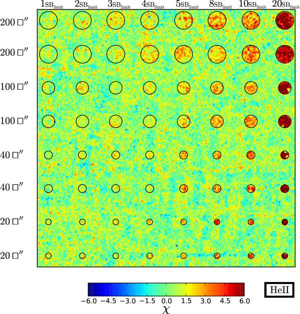
Figure 6.— Illustration of detection significance of the simulated sources as a function of sizes in He II line. The panel shows the $\chi_{smth}$ image for the simulated sources with circular top-hat profile with uniform surface brightness. From top to bottom, the simulated sources are placed as follow: two rows for each area (200, 100, 40, 20 arcsec²) with a surface brightness level of 1, 2, 3, 4, 5, 8, 10, 20 ${\rm SB}_{\rm limit}$. The black circles indicate the position of the simulated sources. Note that we should be able to detect sources down to a sensitivity limit of $5{\rm SB}_{\rm limit}$, which corresponds to SB(HeII) = $5.02\times 10^{-19}$ erg s^-1 cm^-2 arcsec^-2 for an area of 200 arcsec² (i.e. LAB1). The same stretch and color schemes are adopted in Figures 7 and 10.

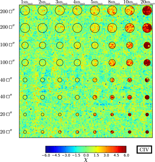
Figure 7.— Illustration of detection significance of the simulated sources as a function of sizes in C IV line. The panel shows the $\chi_{smth}$ image for the simulated sources with circular top-hat profile with uniform surface brightness. From top to bottom, the simulated sources are placed as follow: two rows for each area (200, 100, 40, 20 arcsec²) with a surface brightness level of 1, 2, 3, 4, 5, 8, 10, 20 ${\rm SB}_{\rm limit}$. The black circles indicate the position of the simulated sources. Note that we should be able to detect sources down to a sensitivity limit of $5{\rm SB}_{\rm limit}$, which corresponds to SB(CIV) = $7.36\times 10^{-19}$ erg s^-1 cm^-2 arcsec^-2 for an area of 200 arcsec² (i.e. LAB1). The same stretch and color schemes are adopted in Figures 6 and 10.

Figure 6 and 7 show the $\chi_{\rm smth}$ for the simulated sources for He II and C IV images, respectively. For each detection significance and source size, the simulated sources are shown for two different positions within the He II or the C IV images. To guide the eye, these positions are highlighted by a black circle. These simulated $\chi_{\rm smth}$ images confirm that we should be able to detect extended emission down to a level of $5{\rm SB}_{\rm limit}$, justifying our choice for this detection threshold. Note again that ${\rm SB}_{\rm limit}$ includes the correction we made to take into account the systematics.

In addition to the previous analysis, in order to further test our continuum subtraction, we also performed the continuum subtraction using two off-band images ($V$ and $i^{\prime}$; Hayashino et al. 2004), finding that the results remain unchanged. Note however, that due to the differences in the telescope PSFs and seeing of the observations, the use of two bands increases the noise. Thus, we prefer to estimate the continuum using only the $R$-band image.

3. Observational Results

In Figure 8 and 9, we show the postage-stamp images for the 13 LABs in our sample. Each row displays the $R$-band, the continuum-subtracted Ly$\alpha$ line image, the narrowband image of the C IV $\lambda$1549 line, the continuum-subtracted C IV line image, the He II $\lambda$1640 narrowband image, and the continuum-subtracted He II line image, respectively. The red contours indicate the isophotal aperture of LABs defined as the area above 2$\sigma$ detection limit for the Ly$\alpha$ emission as originally adopted by Matsuda et al. (2004), i.e. $2.2\times 10^{-18}$ erg s^-1 cm^-2 arcsec^-2. The continuum-subtracted C IV and He II line images are nearly flat and lack significant large-scale residuals, indicating good continuum and background subtraction. Note that there could be still some residuals within the isophotal apertures (e.g., LAB2) because of minor mis-alignment between $R$-band and our narrowband images. However, these residuals do not affect our flux and surface brightness measurements. We do not detect any extended C IV or He II emission on the scale of the Ly$\alpha$ line in any of the LABs.

Figure 8.— Postage-stamp images of 30″$\times$ 30″(corresponding to about 230 kpc $\times$ 230 kpc at $z=3.1$) centered on LAB1, LAB2, LAB7, LAB8, LAB11, and LAB12. From left to right: $R$-band, Ly$\alpha$, OI/2500+57 (NB CIV), CIV$\lambda$1549, SII+62 (NB HeII), and HeII$\lambda$1640. On the $R$-band, CIV$\lambda$1549, and HeII$\lambda$1640, is over-plotted the 2$\sigma$ isophotal aperture of the Ly$\alpha$ emission (red line) as adopted by Matsuda et al. (2004). Note the lack of extended emission in the CIV$\lambda$1549 and HeII$\lambda$1640 in comparison with the outstanding Ly$\alpha$ line. North is up, East is left.

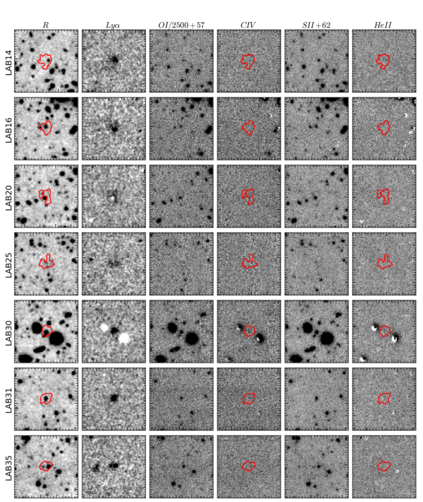
Figure 9.— Postage-stamp images of 30″$\times$ 30″(corresponding to about 230 kpc $\times$ 230 kpc at $z=3.1$) centered on LAB14, LAB16, LAB20, LAB25, LAB30, LAB31, and LAB35. From left to right: $R$-band, Ly$\alpha$, OI/2500+57 (NB CIV), CIV$\lambda$1549, SII+62 (NB HeII), and HeII$\lambda$1640. On the $R$-band, CIV$\lambda$1549, and HeII$\lambda$1640, is over-plotted the 2$\sigma$ isophotal aperture of the Ly$\alpha$ emission (red line) as adopted by Matsuda et al. (2004). Note the lack of extended emission in the CIV$\lambda$1549 and HeII$\lambda$1640 in comparison with the outstanding Ly$\alpha$ line. North is up, East is left.

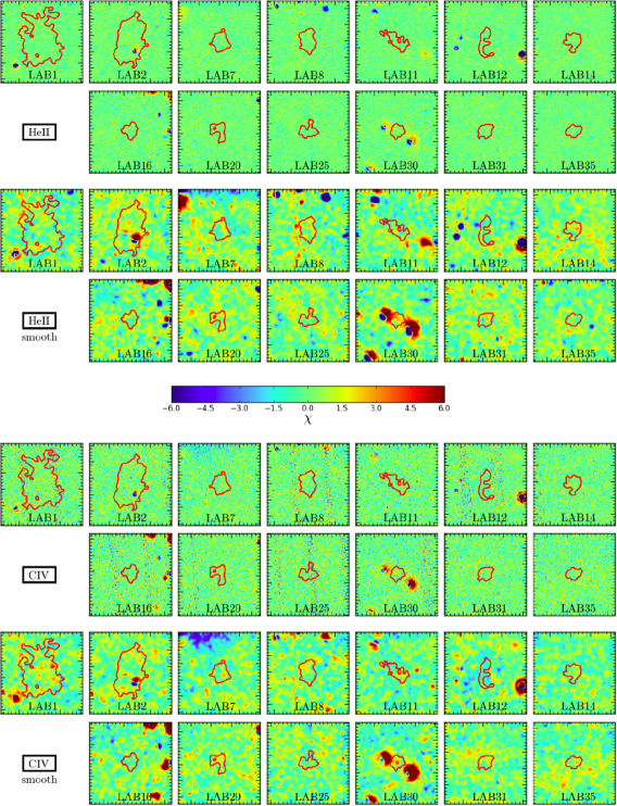
Figure 10.— Postage-stamp $\chi$ and $\chi_{\rm smth}$ images of the 13 LABs in our sample (§2.4). Each postage-stamp has a size of $30\arcsec\times 30\arcsec$ (corresponding to about 230 kpc $\times$ 230 kpc at $z=3.1$). To guide the eye, on each image is overplotted the 2$\sigma$ isophotal aperture of the Ly$\alpha$ emission (red line) as adopted by Matsuda et al. (2004). A comparison with Figures 6-7 suggest that we did not detect any extended emission from any of the sources in our sample. Note that we used the same stretch and colormap as in Figure 6 and 7. Residuals from bright foreground objects due to minor mis-alignment between our data and SUBARU data are clearly visible. North is up, East is left.

In order to better visualize these non-detections, we compute the $\chi$ and $\chi_{\rm smth}$ described in §2.4 for each LAB (using the pure photon counting noise estimates). Figure 10 shows the $\chi$ images and the $\chi_{\rm smth}$ images of $30\arcsec\times 30\arcsec$ (corresponding to 230 kpc $\times$ 230 kpc at $z=3.1$) centered on each LAB. A comparison of the $\chi_{\rm smth}$ images of the individual Ly$\alpha$ blobs with the simulated images in Figures 6 and 7 shows that we do not detect any extended emission in the HeII and CIV lines for the 13 LABs down to our sensitivity limits of $5{\rm SB}_{\rm limit}$ defined in Section §2.4. Note that we show images in Figures 6, 7 and 10 with the same stretch and color scheme for a fair comparison.

We thus place conservative upper limits, i.e. $5{\rm SB}_{\rm limit}$, on both CIV$\lambda$1549 and HeII$\lambda$1640 surface brightness for each of the LABs. For LAB1 (area 200 arcsec²), these limits correspond to SB(He II) = $5.02\times 10^{-19}$ erg s^-1 cm^-2 arcsec^-2 and SB(C IV) = $7.36\times 10^{-19}$ erg s^-1 cm^-2 arcsec^-2. In Table 2, we summarize all of our upper limits, the properties of Ly$\alpha$ lines, and the resulting upper limits on the C IV $\lambda$1549/Ly$\alpha$ and He II $\lambda$1640/Ly$\alpha$ flux ratios. Note that the most stringent limits on these ratios are obtained for the brightest LAB1 and LAB2 given their larger Ly$\alpha$ isophotal area and luminosities. Coincidentally, these two LABs show the same values, $F$(He II)/$F$(Ly$\alpha$) $<$ 0.11 and $F$(C IV)/$F$(Ly$\alpha$) $<$ 0.16, because the difference in the area (LAB1 is larger than LAB2) is compensated by the difference in Ly$\alpha$ SB (LAB2 has a SB higher than LAB1). In what follows, we compare our limits to previous constraints on HeII and CIV in other nebulae, and then discuss the implications of our non-detections.

4. Previous Observations of He II and C IV

We compile He II and C IV line observations of extended Ly$\alpha$ nebulae from the literature, finding data for five Ly$\alpha$ blobs (Dey et al. 2005; Prescott et al. 2009, 2013, summarized in Table 4 in the Appendix), Ly$\alpha$ nebulae associated with 53 high redshift radio galaxies (Humphrey et al. 2006; Villar-Martín et al. 2007), and five radio-loud QSOs (Heckman et al. 1991a, b; Humphrey et al. 2013). However, a straightforward comparison is restrained by the following issues. First of all, these data are obtained with various different techniques (e.g., narrowband imaging, longslit spectroscopy, integral-field unit spectroscopy), and employ varied analysis methods (e.g., different extraction apertures), which result in different definitions of SB limits. Thus, a major uncertainty in comparing our data with the previous measurements are differences in the aperture for which these line fluxes or ratios are reported. In particular, our upper limits are computed over the entire Ly$\alpha$ nebulae defined by the $2\sigma$ Ly$\alpha$ isophotal apertures of Matsuda et al. (2004) (e.g. see Figures 8 and 9), above a Ly$\alpha$ surface brightness limit of $2.2\times 10^{-18}$ erg s^-1 cm^-2 arcsec^-2, and because of the use of narrow-band imaging, we can probe the whole extent of the source. On the other hand, in the case of LABs (Prescott et al. 2013; Dey et al. 2005) and HzRGs (Villar-Martín et al. 2007), the lines are extracted from smaller aperture forcedly defined by the slit, sampling a particular position within the nebula. For example, in the case of HzRGs (De Breuck et al. 2000), the lines are typically measured from a one-dimensional spectra extracted by choosing the aperture which includes the most extended emission line, and typically the slit is oriented along the radio axis.

To further complicate the comparison, for HzRGs and QSOs where a bright central source is clearly detected, it is difficult to separate the emission from the central source and from the nebula itself. For example, for the radio-loud QSOs, Heckman et al. (1991a, b) carefully removed the contribution from the central QSOs in both the imaging and the spectroscopic analysis, thus these line ratios should only reflect the line emission in the extended nebulae. However, in the measurements for HzRGs no attempt is made to exclude a possible contribution from the central obscured AGN. While in the case of the LABs, the neglect of the contribution of the sources within the Ly$\alpha$ emission is not relevant because the star-forming galaxies embedded in the nebulae should scarcely emit in C IV and He II lines (e.g. Shapley et al. 2003), and constitute only a small fraction of the area in the aperture.

Despite these caveats, in Figure 11 we plot all the available data in the literature for completeness to show the ranges spanned by these different types of sources in a He II/Ly$\alpha$ versus C IV/Ly$\alpha$ diagram. But we caution again the reader that a direct comparison of objects from different studies in this plot could be problematic. The upper limits for the 13 Ly$\alpha$ blobs in our sample are shown in red.

Figure 11 illustrates that our upper limits are consistent with the previous measurements and more interestingly, that there are sources in the literature with line ratios even lower than our strongest upper limits (LAB1 and LAB2, gray shaded region). Indeed, although our narrow band images constitute the deepest absolute SB limits ever achieved in the C IV and He II emission lines, some previous searches probed to smaller values of the line ratios because they observed brighter Ly$\alpha$ nebulae (e.g. in the case of HzRGs) or because they probed only the central part of the nebula where the Ly$\alpha$ emission is expected to be brighter. For example, Prescott et al. (2013) probed down to lower line ratios (e.g. the lowest green point in the plot, i.e. the LAB PRG2) because they focus on the brightest part of the blob in Ly$\alpha$. Indeed, while the approximate isophotal area for this LAB is 103 arcsec², they covered only a smaller aperture (1.5″$\times$7.84″) with their long-slit spectra. Thus, notwithstanding our efforts, Figure 11 is clearly indicating that in order to explore the full range of line ratios, one requires either deeper observations, or brighter samples of Ly$\alpha$ emission nebulae (see e.g. Cantalupo et al. 2014).

In addition to the sources with giant Ly$\alpha$ emission nebulae, Figure 11 also shows line ratios for star-forming galaxies at $z=2-3$, for which the CIV and HeII line ratio is not powered by an AGN. In particular, we show the line ratios determined from the composite spectrum of Lyman break galaxies (LBGs) from Shapley et al. (2003) and for a peculiar galaxy (Q2343-BX418) studied in detail by Erb et al. (2010) which exhibits particularly strong He II emission. We show the corresponding line-ratios for LBGs because it has been proposed that some LABs could be powered by star-formation
(Ouchi et al. 2009), albeit with extreme star-formation rates $\simeq 1000\,{\rm M}_{\odot}/{\rm yr}$. Indeed, the stacked Ly$\alpha$ narrowband images of LBGs also exhibit diffuse Ly$\alpha$ emission extending as far as $\sim$50 kpc (Steidel et al. 2011), although the Ly$\alpha$ luminosity and surface brightness of these halos is $\gtrsim 10\times$ fainter than the LABs and the Ly$\alpha$ nebulae associated with HzRGs and QSOs. However, if the LABs represent some rare mode of spatially extended star-formation, then the C IV and He II line ratios of star-forming galaxies could thus be relevant.

The origin of the He II and C IV emission observed in the spectra of star-forming galaxies is not completely understood. Shapley et al. (2003) noted relatively broad (FWHM $\sim$1500 km s^-1) He II emission in the composite spectrum of LBGs, and speculated that it arises from the hot, dense stellar winds of Wolf-Rayet (W-R) stars, which descend from O stars with masses of $M$ $>$ 20–30 M_⊙. The C IV line in LBGs exhibits a characteristic P Cygni-type profile, which presumably arises from a combination of stellar wind and photospheric absorption, plus a strong interstellar absorption component due to outflows (Shapley et al. 2003). There could also be a narrow nebular emission component powered by a hard ionizing source. In Figure 11 we adopt the strict upper limit of C IV/Ly$\alpha$ $<0.02$ of the non-AGN subsample in Shapley et al. 2003, whereas for the He II/Ly$\alpha$ ratio we use the global value for the first quartile with the Ly$\alpha$ line in emission because no He II/Ly$\alpha$ value was quoted for the non-AGN subsample. Erb et al. (2010) studied a young ($<100$Myr), low metallicity ($Z\sim 1/6Z_{\odot}$) galaxy at $z=2.3$ which exhibits exceptionally strong He II emission, which they however argued is not powered by an AGN. Erb et al. (2010) interpreted the He II emission as a combination of a broad component due to W-R stars and a narrow nebular component, powered by a hard ionizing spectrum. Although the He II emission is strong in comparison with other typical $z\sim 2-3$ LBGs, indicative of a harder ionizing spectrum, the He II/Ly$\alpha$ ratio of this galaxy is in fact lower than that of the average LBG owing to its extremely strong Ly$\alpha$ line.

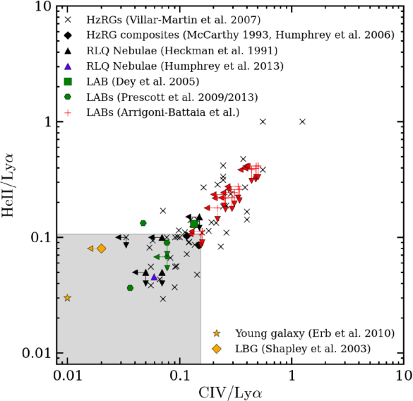
Figure 11.— HeII/Ly$\alpha$ versus CIV/Ly$\alpha$ log-log plot. Our upper limits on the HeII/Ly$\alpha$ and CIV/Ly$\alpha$ ratios are compared with the values quoted in the literature for HzRG, QSOs, and LABs (see text for references). Due to their larger extent, LAB1 and LAB2 define the strongest limits on these ratios: the gray shaded area highlights the regime constrained by these limits. Note however that these data are quite difficult to compare because of their heterogeneity.

5. Discussion

In what follows we discuss our upper limits in light of a photoionization or a shock scenario. Here, we briefly outline the physics underlying the models and the parameters used, but we refer the reader to Hennawi & Prochaska (2013) and our subsequent paper (Arrigoni-Battaia et al. in prep.) for further details and a complete analysis.

5.1. Comparison with Photoionization Models

It is well established that the ionizing radiation from a central AGN can power giant Ly$\alpha$ nebulae, with sizes up to $\sim$ 200 kpc, around high-z radio galaxies (HzRG) (e.g., Villar-Martín et al. 2003b; Reuland et al. 2003; Venemans et al. 2007) and quasars (e.g., Heckman et al. 1991b; Christensen et al. 2006; Smith et al. 2009), together with extended He II and C IV emission (Villar-Martín et al. 2003a). Although HzRGs are more rare ($n\sim 10^{-8}$ Mpc^-3; Miley & De Breuck 2008), the similarity between the volume density of LABs ($n\sim 10^{-5}$ Mpc^-3; Yang et al. 2010) and luminous QSOs ($n\sim 10^{-5}$ Mpc^-3; Hopkins et al. 2007), suggests that the LABs could represent the same photoionization process around obscured QSOs. Unified models of AGN invoke an obscuring medium which could extinguish a bright source of ionizing photons along our line of sight (e.g., Urry & Padovani 1995). Indeed, evidence for obscured AGNs have been reported for several LABs (e.g., Basu-Zych & Scharf 2004; Dey et al. 2005; Geach et al. 2007; Barrio et al. 2008; Geach et al. 2009; Overzier et al. 2013; Yang et al. 2014a), lending credibility to a photoionization scenario; however, this is not always the case (Nilsson et al. 2006; Smith & Jarvis 2007; Ouchi et al. 2009).

Despite these circumstantial evidences in favor of the photoionization scenario, detailed modeling for He II and C IV lines due to AGN photoionization in the context of large Ly$\alpha$ nebulae has not been carried out in the literature, with the exceptions of some studies focusing on the modeling of emission lines in the case of extended emission line regions (EELR) of HzRGs (e.g., Humphrey et al. 2008). Although many authors have modeled the narrow-line regions (NLR) of AGNs (e.g., Groves et al. 2004, Nagao et al. 2006, Stern et al. 2014), the physical conditions on these small scales $\sim 100$ pc (i.e. gas density, ionization parameter) are expected to be very different than the $\sim 100$ kpc scale emission of interest to us here. As such, we model the photoionization of gas on scales of $100$ kpc from a central AGN to predict the resulting level of the He II and C IV lines, relative to the Ly$\alpha$ emission.

To select the parameters of the models in order to recover the Ly$\alpha$ SB of LABs, we follow the simple picture described by Hennawi & Prochaska (2013), and assume a LAB to be powered by an obscured QSO with a certain luminosity at the Lyman limit ($L_{\nu_{\rm LL}}$). In this picture, the QSO halo is populated with spherical clouds of cool gas ($T\sim 10^{4}$ K) at a single uniform hydrogen volume density $n_{\rm H}$ and with an average column density $N_{\rm H}$, and uniformly distributed throughout a halo of radius $R$, such as they have a cloud covering factor $f_{C}$ (see Hennawi & Prochaska 2013 for details). We consider two limiting regimes for recombination: the optically thin ($N_{\rm HI}<10^{17.2}$ cm^-2) and thick ($N_{\rm HI}>10^{17.2}$ cm^-2) to the Lyman continuum photons, where $N_{\rm HI}$ is the neutral column density of a single spherical cloud. In this scenario, once the size of the halo is fixed, in the optically thick case the Ly$\alpha$ surface brightness scales with the luminosity at the Lyman limit of the central source, $SB_{{\rm Ly}\alpha}^{\rm thick}\propto f_{C}L_{\nu_{\rm LL}}$, while in the optically thin regime ($N_{\rm HI}<10^{17.2}$ cm^-2) the SB does not depend on $L_{\nu_{\rm LL}}$, $SB_{{\rm Ly}\alpha}^{\rm thin}\propto f_{C}n_{\rm H}N_{\rm H}$, provided the AGN is bright enough to keep the gas in the halo ionized.

To cover the full range of possibilities, we thus construct a grid of $\sim$5000 Cloudy models with parameters in the following range (see the appendix for additional information on how the parameters were chosen):

• $n_{\rm H}=0.01$ to $100$ cm^-3 (steps of 0.2 dex);

• $\log N_{\rm H}=18$ to $22$ (steps of 0.2 dex);

• $\log L_{\nu_{\rm LL}}=29.3$ to $32.2$ (steps of 0.4 dex).

Finally, we decide to fix the covering factor to unity $f_{C}=1.0$. The assumption of a high or unit covering factor is driven by the observed diffuse morphology of the Ly$\alpha$ nebulae, which do not show evidence for clumpiness arising from the presence of a population of small unresolved clouds. We directly test this assumption as follows. We randomly populate an area of 200 arcsec² (area of LAB1) with point sources such that $f_{C}=0.1-1.0$, and we convolve the images with a Gaussian kernel with a FWHM equal to our median seeing value, in order to mimic the effect of seeing in the observations. We find that the smooth morphology observed for LABs cannot be reproduced by images with $f_{C}<0.5$, as they appear too clumpy.

We preform photoionization calculations using the Cloudy photoionization code (v10.01), last described by Ferland et al. (2013). As the LABs are extended over $\sim 100$ kpc, whereas the radius of the emitting clouds is expected to be much smaller, we assume a standard plane-parallel geometry for the emitting clouds illuminated by the distant central source. Note that we evaluate the ionizing flux at a single location for input into Cloudy, specifically at $R/\sqrt{3}$ (where $R=100$ kpc). Capturing the variation of the physical properties of the nebula with radius is beyond the purpose of this work. Indeed, given that for the objects in the literature are not reported radial trends for the C IV/Ly$\alpha$ and He II/Ly$\alpha$ ratios, and given that we have non detections, modeling the emission as coming from a single radius is an acceptable first order approximation. We consider only models with solar metallicity, and we assume that the ionizing continuum has a power law form $L_{\nu}=L_{\nu_{\rm LL}}(\nu/\nu_{\rm LL})^{\alpha}$, where $\nu_{\rm LL}$ is the frequency of the Lyman limit, and we take the slope of the ionizing continuum set to be $\alpha_{EUV}=-1.57$ following Telfer et al. (2002). Note that our assumption of this power law ionizing continuum amounts to assuming that the central AGN powering the LAB has a spectrum similar to a Type-1 QSO; of course this UV ionizing source is not directly observed because it is presumed to be obscured from our vantage point. Note that unlike the case where a QSO is clearly powering a nebula, for LABs we do not have a constraint on the ionizing luminosity of the central source $L_{\nu_{\rm LL}}$. As we have assumed that a Type-1 QSO spectrum powers the nebulae, we can convert $L_{\nu_{\rm LL}}$ into an $i$-band apparent magnitude following the procedure described in Hennawi et al. (2006). The $L_{\nu_{\rm LL}}$ that we consider correspond to $i$-band apparent magnitudes of $i=16-23$, in steps of unity.

In addition to the Ly$\alpha$ due to the recombination, the resonant scattering of Ly$\alpha$ becomes important when the gas is optically thick at Ly$\alpha$ line, roughly for $N_{\rm HI}\gtrsim 10^{14}$ cm^-2. The Ly$\alpha$ emission from scattering will follow the relation (Hennawi & Prochaska 2013)

$$SB_{{\rm Ly}\alpha}^{\rm scatt}=\frac{h\nu_{{\rm Ly}\alpha}}{4\pi(1+z)^{4}}f_{\rm C}\Phi_{{\rm Ly}\alpha}(R/\sqrt{3}),$$ (6)

where $\Phi_{{\rm Ly}\alpha}$ is the flux of continuum photons emitted close enough to the Ly$\alpha$ resonance to be scattered by gas in motion around the quasar (we assume that the rest-frame equivalent width of Ly$\alpha$ absorption is close to 1 Å, Hennawi & Prochaska 2013). To take into account this effect, we simply add this scattering contribution to the photoionization Ly$\alpha$ SB of the models. Note that the scattering emission is not relevant in the optically thick regime because the flux of ionizing photons is larger than the flux of Lya photons, i.e. $\Phi_{\rm LL}/\Phi_{{\rm Ly}\alpha}\sim 150$ (Hennawi & Prochaska 2013). On the other hand, in the case of the optically thin regime, the SB_Lyα for scattering is comparable with the emission from the recombination if the central source is bright enough (in this work for $i<18$). Finally, from our model grid, we select only models with SB_Lyα = (1–9)$\times$$10^{-18}$ erg s^-1 cm^-2 arcsec^-2, comparable to LABs.

In Figure 12 we compare our photoionization model predictions in the He II/Ly$\alpha$ versus C IV/Ly$\alpha$ diagram to our LAB limits and the data points from the literature. The left panel and right panels show the optically thin and optically thick regimes, respectively. Note that this division into optically thin and thick models, corresponds to a division in the ionizing luminosity of the central source (which in the case of LABs and HzRGs is obscured from our vantage point and is thus unknown). Specifically, in the optically thin regime we find that for the range of ${\rm SB}_{\rm Ly\alpha}$ considered, the central source must have $L_{\nu_{\rm LL}}\gtrsim 10^{30.5}$ erg s^-1 Hz^-1 or $i\lesssim 20$ . On the other hand, because in the optically thick limit ${\rm SB}_{\rm Ly\alpha}\propto L_{\nu_{\rm LL}}$, the ionizing luminosity is fixed to be in a relatively narrow range $L_{\nu_{\rm LL}}\simeq 10^{29.7}-10^{29.3}$ erg s^-1 Hz^-1 ($i\simeq 22-23$).

For clarity, in Figure 12 we show only the models with $N_{\rm H}=10^{19},10^{20},10^{21},10^{22}$ cm^-2. The model grids are color-coded according to the ionization parameter $U$, which is defined to be the ratio of the number density of ionizing photons to hydrogen atoms ($U\equiv\Phi_{LL}/cn_{\rm H}\propto L_{\nu_{\rm LL}}/n_{\rm H}$), and provides a useful characterization of the ionization state of the nebulae. Because photoionization models are self-similar in this parameter (Ferland, 2003), our models will exhibit a degeneracy between $n_{\rm H}$ and $L_{\nu_{\rm LL}}$. Nevertheless, we decided to construct our model grid in terms of $N_{\rm H}$ and $L_{\nu_{\rm LL}}$, in order to explore the possible ranges of both parameters.

Figure 12 illustrates that, overall, our photoionization models can cover the full range of HeII/Ly$\alpha$ and CIV/Ly$\alpha$ line ratios that are observed in the data. The optically thin regime (see left panel) seems to better reproduce the range of line ratios set by our most stringent upper limits (LAB1 and LAB2), as well the locus of measurements in the C IV/Ly$\alpha$– He II/Ly$\alpha$ diagram for HzRGs, QSOs, and LABs. In particular, models with log$U\approx-1.5$ and $10^{19}\leq N_{\rm H}<10^{20}$ cm^-2 populate the region below our LAB limits, whereas models with log$U\gtrsim-2.0$ and $10^{19}\leq N_{\rm H}<10^{21}$ cm^-2 would be broadly consistent with most of the detections. Note that previous studies of EELR around HzRGs favored models with log$U\sim-1.46$ (e.g. Humphrey et al. 2008), which are consistent with our results.

Note however that two HzRGs with He II/Ly$\alpha$ $\approx$ 1 and C IV/Ly$\alpha$ $\approx$ 1, are not covered by our models. For both of these data, emission from the central source has not been excluded, and thus we speculate that these very high line ratios arise because of contamination from the narrow-line region of the obscured AGN, where Ly$\alpha$ photons have been destroyed by dust. Indeed, both of these objects, MG1019+0535 and TXS0211-122, have a C IV/He II ratio similar to the bulk of the HzRGs population, but they exhibit unusually weak Ly$\alpha$ lines (Dey et al. 1995, van Ojik et al. 1994). Note however, that while destruction of Ly$\alpha$ by dust grains can have a large impact on these line ratios for emission emerging from the much smaller scale narrow line region, dust is not expected to significantly attenuate the Ly$\alpha$ emission in the extended nebulae around QSOs (see discussion in Appendix A of Hennawi & Prochaska 2013) given the physical conditions characteristic of the CGM, and thus we neglect destruction of Ly$\alpha$ photons by dust in our modeling.

The trajectory of the optically thin models through the HeII/Ly$\alpha$ and CIV/Ly$\alpha$ diagram can be understood as follows. We first focus on the curve for $N_{\rm H}=10^{19}\,{\rm cm^{-2}}$ and follow it from low to high $U$. Recall that in the optically thin regime $SB_{Lya}\propto n_{\rm H}N_{\rm H}$, but is roughly independent of the source luminosity $L_{\nu_{\rm LL}}$ . Thus by fixing $N_{\rm H}=10^{19}\,{\rm cm^{-2}}$, and requiring that $SB_{{\rm Ly}\alpha}=$(1–9)$\times 10^{-18}$ erg s^-1 cm^-2, we also fix $n_{\rm H}$. Thus $U$ is increases along this track because the central source luminosity is increasing $L_{\nu_{\rm LL}}$, which hardly changes the Ly$\alpha$ emission, but results in significant variation in both He II and C IV.

First consider the trend of the He II/Ly$\alpha$ ratio. He II is a recombination line and thus, once the density is fixed, its emission depends basically on what fraction of Helium is doubly ionized. For this reason, the He II/Ly$\alpha$ ratio is increasing from log$U=-3.3$ and reaches a peak at log$U\sim-2.0$, corresponding to an increase in the fraction of the He⁺⁺ phase from about 20% to 90% of the total Helium. Further increases $U$, result in only modest changes to the He⁺⁺ fraction, but result in an increase in gas temperature. These higher temperatures result in a decrease of the He⁺⁺ recombination rate. In addition this higher temperature impacts the Ly$\alpha$ line in the same way, but continuum pumping due to the increased luminosity of the central source further increases the Ly$\alpha$ emission, with the net effect that He II emission is reduced relative to Ly$\alpha$ (as discuss in Arrigoni-Battaia et al. in prep.).

Our photoionization models indicate that the C IV emission line is an important coolant and is powered primarily by collisional excitation. Figure 12 shows that our models span a much wider range in the C IV/Ly$\alpha$ ($\sim 3$ dex) ratio than in He II/Ly$\alpha$ ($\lesssim 2$ dex). The strong evolution in C IV/Ly$\alpha$ results from a combination of two effects. First, increasing $U$ increases the temperature of the gas, and the C IV collisional excitation rate coefficient has a strong temperature dependence (Groves et al. 2004). Second, the efficacy of C IV as a coolant depends on the amount of Carbon in the C⁺³ ionic state. As log$U$ increases from $\simeq-3.3$ to $\simeq-2$, the C⁺³ fraction increases from 1% to 37%. These two effects conspire to give rise to nearly three orders of magnitude of variation in the C IV emission.

Although our analysis suggests that the optically thin models are favored, the optically thick models (see right panel of Figure 12) can also populate the area below the upper limits for LAB1 and LAB2, and at least the lower part of the observed He II/Ly$\alpha$ – C IV/Ly$\alpha$ diagram. Note that given the range of $L_{\nu_{\rm LL}}$ and $n_{\rm H}$ in our parameter grid, models with $N_{\rm H}=10^{19}$ cm^-2 are never optically thick, which explains why we only show optically thick models with $N_{\rm H}=10^{20},10^{21},10^{22}$ cm^-2. The bulk of these models reside on a sequence with almost constant HeII/Ly$\alpha$ (around HeII/Ly$\alpha=0.04-0.05$) for a wide range of CIV/Ly$\alpha$, which is driven by variation in $U$. The models departing from this sequence are characterized by $N_{\rm HI}$ slightly greater than $10^{17.2}$ cm^-2 and they can thus be seen as a transition between the optically thick case and the optically thin case.

To summarize, the photoionization models produce line ratios which are consistent with our upper limits and which span the values observed in the literature, although we favor the optically thin scenario. In the next section we consider the degree to which shock powered emission can explain line ratios in Ly$\alpha$ nebulae.

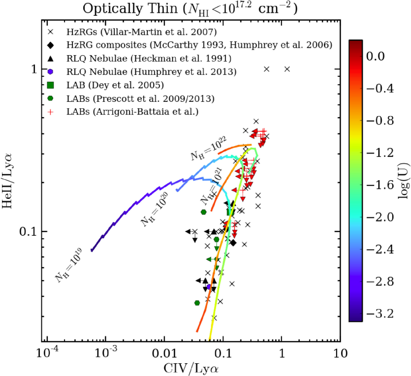
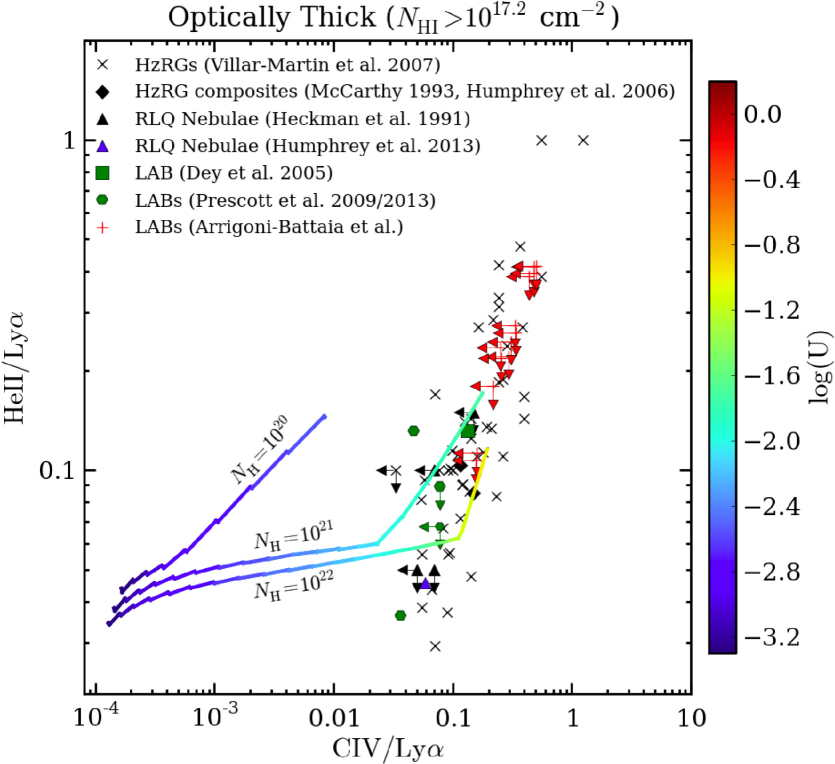
Figure 12.— HeII/Ly$\alpha$ versus CIV/Ly$\alpha$ log-log plot. Same data points as in Figure 11. Our upper limits on the HeII/Ly$\alpha$ and CIV/Ly$\alpha$ ratios are compared with the Cloudy photoionization models. In the left panel we plot the optically thin models, while in the right panel is shown the optically thick regime. For clarity, we plot only the models with $N_{\rm H}=10^{19},10^{20},10^{21},10^{22}$ cm^-2. The grids are color coded following the ionization parameter (see colorbar on the right) and the value of hydrogen column density is indicated. Note that there are no optically thick models with $N_{\rm H}=10^{19}$ cm^-2. Note that the x-axis is on different scale than Figure 11.

5.2. Comparison with Shock Models

Taniguchi & Shioya (2000) and Mori & Umemura (2006) have speculated that intense star-formation accompanied by successive supernova explosions could power a large scale galactic superwind, and radiation generated by overlapping shock fronts could power the Ly$\alpha$ emission in the LABs. However, it is well known that it is difficult to distinguish between photoionization and fast-shocks using line-ratio diagnostic diagrams (e.g. Allen et al. 1998). Furthermore, for AGN narrow line regions, the Ly$\alpha$ line is typically avoided in these diagrams because of its resonant nature and the fact that it may be more likely to be destroyed by dust, although we have argued that it is not an issue for CGM gas. It is thus interesting to study how shock models populate the He II/Ly$\alpha$ versus C IV/Ly$\alpha$ diagram in comparison with photoionization models and our observational limits.

To build intuition about the line ratios expected in a shock scenario we rely on the modeling of fast shocks by Allen et al. (2008). We thus imagine the Ly$\alpha$ emission as the sum of overlapping shock fronts with shock velocity $v_{\rm s}$, moving into a medium with preshock density $n_{\rm H}$. In the case of such shocks, Allen et al. (2008) showed that the Ly$\alpha$ emission depends strongly on $v_{\rm s}$, i.e. $F_{{\rm Ly}\alpha}\propto n_{\rm H}v_{s}^{3}$ (their Table 6). In order to test a realistic set of parameters in the case of LABs, we limit the grid of models presented by Allen et al. (2008) to:

• $n_{\rm H}=0.01,0.1,1.0,10,100$ cm^-3,

• shock velocities, $v_{\rm s}$, from 100 km s^-1 to 1000 km s^-1 in steps of 25 km s^-1.

We consider only models with solar metallicity . The magnetic parameter $B/n^{1/2}$, where B is the magnetic field in $\mu$G, determines the relative strength of the thermal and magnetic pressure. We adopt a magnetic parameter $B/n^{1/2}=3.23$ $\mu$G cm^3/2, which represents a value expected for ISM gas assuming equipartition of magnetic and thermal energy. However, note that, given the very strong dependence of the ionizing flux on the shock velocity $F_{\rm UV}\propto v_{\rm s}^{3}$, the line ratios do not vary so markedly with either the metallicity or the magnetic field (see Allen et al. 2008 for further details).

In Figure 13 we show two sets of shock models. On the left, we plot the models for which the emission is coming solely from the shocked region, where the gas is ionized and excited to high temperatures by the shock. Temperatures ahead of the shock-front are of the order of 10⁴ K , whereas temperatures as high as 10⁶ K can be reached in the post-shock gas (Allen et al. 2008). On the right, we plot a combination of the emission coming from the shocked gas and from the precursor, i.e. the pre-shock region which is photoionized by the radiation emitted upstream from the shocked region. The trends of the models can be explained as follows. The models for the shock component (left panel of Figure 13) show a rapid decrease in the C IV/Ly$\alpha$ ratio for increasing $v_{\rm s}$. This is due to a rapid increase in the Ly$\alpha$ line due to the strong scaling of the ionizing flux with $v_{\rm s}$, and to a decrease in the CIV line due to the lack of carbon in the C³⁺ phase for high velocities (i.e. carbon is in higher ionization species, see Figure 9 of Allen et al. 2008). The He II/Ly$\alpha$ ratio depends more strongly on the gas density because $n_{\rm H}$ sets the volume of the shocked region and thus the recombination luminosity of Helium, i.e. at fixed $v_{\rm s}$, a higher density corresponds to a smaller shocked volume and less Helium emission (see Figure 6 of Allen et al. 2008).

The combination of shock and precursor models mainly alter the ratios for models with high $v_{\rm s}$ (see right panel of Figure 13). This is because the precursor component is adding the contribution of a photoionized gas at temperature of the order of 10⁴ K, and the ionizing flux scales strongly with shock velocity $F_{\rm UV}\propto v_{\rm s}^{3}$. For velocities $v_{\rm s}\gtrsim 400$ km s^-1, the resulting hard radiation field results in a large fraction of double ionized Helium He⁺⁺ over a significant volume of the precursor, significantly increasing the He II emission and the He II/Ly$\alpha$ ratio. This photoionized precursor similarly increases the abundance of the C³⁺ phase giving rise to a higher C IV/Ly$\alpha$ ratio. Thus, adding the precursor contribution to the shock models causes the models to fold over each other at high velocities.

Figure 13 illustrates that the shock models are capable of populating the line ratio diagram below our tightest upper limits (i.e. LAB1 and LAB2). However, note that our limits on the C IV line imply velocities above $\sim$250 km s^-1, in potential disagreement with independent constraints on the outflow velocities in LABs in the literature. Indeed, using the velocity offset between the Ly$\alpha$ and the non-resonant [O III] or H$\alpha$ line, the offset of stacked interstellar metal absorption lines, and the [O III] line profile, Yang et al. (2011, 2014b) find that the kinematics of gas along the line of sight to galaxies in LABs are consistent with a simple picture in which the gas is stationary or slowly outflowing at a few hundred km s^-1 from the embedded galaxies in contrast with the $\sim$1000 km s^-1 velocities necessary to power LABs via superwind outflows (Taniguchi & Shioya 2000). In addition, Prescott et al. (2009) showed that the He II line detected for a LAB at $z=1.67$, is narrow, i.e. $v_{\rm FWHM}\lesssim 500$ km s^-1. If shocks are the mechanism powering the nebula, this observation is inconsistent with strong shock velocities, i.e. $v_{\rm s}\lesssim 500$ km s^-1. Thus, these observations seem to rule out an extreme wind scenario in these LABs.

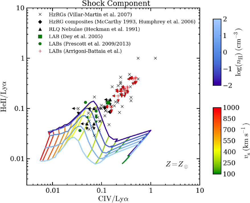
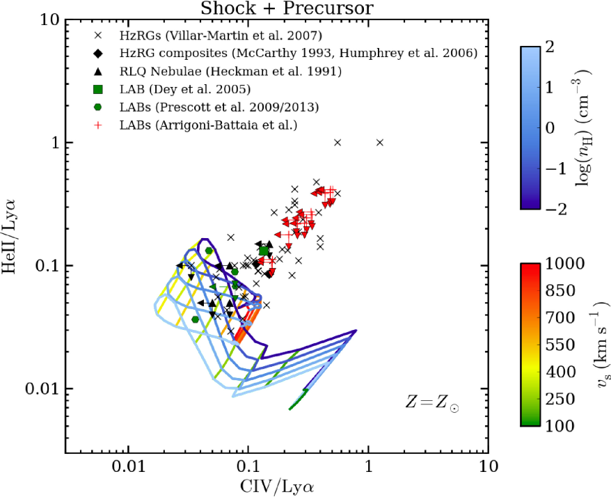
Figure 13.— HeII/Ly$\alpha$ versus CIV/Ly$\alpha$ log-log plot. Same data points as in Figure 11. Our upper limits on the HeII/Ly$\alpha$ and CIV/Ly$\alpha$ ratios are compared with the models by Allen et al. (2008). In the left panel we plot the shock models, while in the right panel is shown the combination of shock and precursor. The grids are color coded following the density of the pre-shock region, $N_{\rm H}$, and the velocity of the shock, $v_{\rm s}$. The models are not taking into account the possible additional contribution due to Ly$\alpha$ scattering.

It is worth to stress again here, that these models suffer from uncertainty in the Ly$\alpha$ calculation. In particular, the additional contribution from scattering is not taken into account, thus making the Ly$\alpha$ line weaker. As a consequence, these grids may be shifted to lower values on both axes. Note also that we fix the metallicity to the solar value. However, a decrease in the C IV emission is expected for sub-solar metallicity, weakening the constraints on the shock velocities. The trends with metallicity are beyond the scope of this work and we are going to address them in a subsequent paper (Arrigoni-Battaia et al. in prep.). Thus, even though our models can give us a rough idea of the line emission in the shock scenario, these plots should be treated with caution.

5.3. Comparison to Previous Modeling of Extended Ly$\alpha$ Emission Nebulae

As stated in the previous sections, rigorous modeling of photoionization of large Ly$\alpha$ nebulae in the context of LABs has never been performed. However, Prescott et al. (2009) reported a detection of extended HeII and modeled simple, constant density gas clouds assuming illumination from an AGN, Pop III, and Pop II stars. They are not quoting all the parameters of their Cloudy models (e.g., $N_{\rm H}$) and thus it is not possible to make a direct comparison. However, they found that the data are in agreement with photoionization from a hard ionizing source, either due to an AGN or a very low metallicity stellar population ($Z<10^{-2}-10^{-3}Z_{\odot}$). They conclude that, in the case of an AGN, this source must be highly obscured along the line of sight. They also showed that their observed ratios are inconsistent with shock ionization in solar metallicity gas.

On smaller scales, photoionization has been modeled in the case of EELR of HzRGs. In particular, Humphrey et al. (2008) using the code MAPPINGS Ic (Binette et al. 1985), shows that the data are best described by AGN photoionization with the ionization parameter U varying between objects, in a range comparable with our grid. However, they found that a single-slab photoionization model is unable to explain adequately the high-ionization (e.g. N V) and low-ionization (e.g. C II], [N II], [O II]) lines simultaneously, with higher U favored by the higher ionization lines. They also demonstrated that shock models alone are overall worse than photoionization models in reproducing HzRGs data. In the shock scenario is required an additional source of ionizing photons, i.e. the obscured AGN, in order to match most of the line ratios studied by Humphrey et al. (2008). However, note that shock with precursor models can explain some ratios, e.g. N V/N IV], which are hardly explained by a single-slab photoionization model (Humphrey et al. 2008).

6. Summary and Conclusions

We obtained the deepest ever narrowband images of He II and C IV emission from 13 Ly$\alpha$ blobs in the SSA22 proto-cluster region to study the poorly understood mechanism powering the Ly$\alpha$ blobs. By exploiting the overdensity of LABs in the SSA22 field, we were able to conduct the first statistical multi emission line analysis for a sample of 13 LABs, and compared their emission line ratios to Ly$\alpha$ nebulae associated with other Ly$\alpha$ blobs, high-z radio galaxies (HzRGs), and QSOs. We compared these results to detailed models of He II/Ly$\alpha$ and C IV/Ly$\alpha$ line ratios assuming that the Ly$\alpha$ emission is powered by a) photoionization from an AGN (including the contribution of scattering) or b) in a shock scenario. The primary results of our analysis are:

• We do not detect extended emission in the He II and C IV lines in any of the 13 LABs down to our sensitivity limits, $2.1\times$ and $3.4\times 10^{-18}$ erg s^-1 cm^-2 arcsec^-2 (5$\sigma$ in 1 arcsec²) for He II and C IV, respectively.

• Our strongest constraints on emission line ratios are obtained for the brightest LABs in our field (LAB1 and LAB2), and are thus constrained to be lower than 0.11 and 0.16 ($5\sigma$), for HeII/Ly$\alpha$ and CIV/Ly$\alpha$, respectively.

• Photoionization models, accompanied by a reasonable variation of the parameters ($N_{\rm H}$, $n_{\rm H}$, $i$) describing the gas distribution and the ionizing source, are able to produce line ratios smaller than our upper limits in the HeII/Ly$\alpha$ versus CIV/Ly$\alpha$ diagram. Although our data constitute the deepest ever observations of these lines, they are still not deep enough to rule out photoionization by an obscured AGN as the power source in LABs. These same photoionization models can also accommodate the range of line ratios in the literature for other Ly$\alpha$ nebulae. Models with a population of optically thin clouds $N_{\rm HI}<10^{17.2}\,{\rm cm^{-2}}$ seem to be favored over optically thick models $N_{\rm HI}>10^{17.2}\,{\rm cm^{-2}}$. In particular, optically thin models with log$U\approx-1.5$ and $10^{19}\leq N_{\rm H}<10^{20}$ cm^-2 populate the region below our LAB limits, whereas models with log$U\gtrsim-2.0$ and $10^{19}\leq N_{\rm H}<10^{21}$ cm^-2 would be broadly consistent with most of the HeII and CIV detections in the literature.

• Shock models can populate a HeII/Ly$\alpha$ versus CIV/Ly$\alpha$ diagram below our LAB limits only if high velocity are assumed, i.e. $v_{\rm s}\gtrsim 250$ km s^-1, but they do not reproduce the higher line ratios implied by detections of HeII and CIV in the HzRGs. Observations of relatively weak outflow kinematics in the central galaxies embedded in LABs appear to rule out such high shock velocities (Prescott et al. 2009; Yang et al. 2011, 2014b).

Deeper observations of the HeII and CIV emission lines in the SSA22 field are required in order to make more definitive statements about the mechanism powering the LABs. For example, our photoionization modeling suggests that line ratios as low as HeII/Ly$\alpha$ $\simeq 0.05$ and CIV/Ly$\alpha$ $\simeq 0.07$ can be produced by combinations of physical parameters ($N_{\rm H}=10^{19}-10^{20}$ cm^-2, $n_{\rm H}=1-10$ cm^-3, $i=17$) which are still plausible. This implies that SBs as low as $1\times$ and $1.5\times 10^{-18}$ erg s^-1 cm^-2 arcsec^-2 per 1 arcsec² aperture (5$\sigma$) must be achieved to start to rule out photoionization. For bright giant Ly$\alpha$ nebulae around QSOs, as have been recently discovered (Cantalupo et al. 2014), photoionization modeling are much more constrained, because the ionizing luminosity of the central source is known. Sensitive measurements of line ratios from deep observations can thus constrain the properties of gas in the CGM, as we will discuss in a future paper (Arrigoni-Battaia in prep.). These questions will be addressed by a new generation of image-slicing integral field units, such as the Multi Unit Spectroscopic Explorer (MUSE, Bacon et al. 2004) on VLT or the Keck Cosmic Web Imager (KCWI). By probing an order of magnitude deeper than our current observations, this new instrumentation will usher in a new era of emission studies of the CGM. This unprecedented sensitivity combined with the modeling methodology described here, will constitute an important step forward in solving the mystery of the LABs.

Appendix A Previous observations of He II and C IV in extended Ly$\alpha$ nebulae.

In Table 4, we compile the previous observations of He II and C IV in extended Ly$\alpha$ nebulae.

Table 4Properties of He II and C IV emission from LABs in the literature.

Object	F (Ly$\alpha$)	SB (Ly$\alpha$)	Max. extent	F (CIV)	F (HeII)	Aperture	Reference
	(1)	(2)	(3)	(4)	(5)	(6)
LABd05a	28.9(NB)/3.10 (spectrum)	9.20/45.9	20	0.42	0.41	4.5$\arcsec\times$ 1.5$\arcsec$	Dey et al. 2005
PRG1	4.36	58.1	5.0	0.21	0.57	5.0$\arcsec\times$ 1.5$\arcsec$	Prescott et al. 2009
PRG2	4.92	41.8	7.84	0.18	0.18	7.84$\arcsec\times$ 1.5$\arcsec$	Prescott et al. 2013
PRG3	1.02	12.1	5.60	$<$0.08	$<0.09$	5.60$\arcsec\times$ 1.5$\arcsec$	Prescott et al. 2013
PRG4	1.03	40.9	1.68	$<$0.08	0.07	1.68$\arcsec\times$ 1.5$\arcsec$	Prescott et al. 2013

Note. — (1) Ly$\alpha$ line flux in $10^{-16}$ erg s^-1 cm^-2, (2) Ly$\alpha$ surface brightness in $10^{-18}$ erg s^-1 cm^-2 arcsec^-2, (3) maximum extent in arcsec. (4) C IV line flux in $10^{-16}$ erg s^-1 cm^-2 arcsec^-2, (5) He II line flux in $10^{-16}$ erg s^-1 cm^-2 arcsec^-2. (6) Apertures used to extract the values by the authors in the references.

Appendix B Photoionization Modeling

In this work we have presented results of photoionization models of LABs. A complete description and more detailed analysis of dependence of our models on the input parameters will be presented in a future paper (Arrigoni-Battaia in prep.). In this Appendix, we provide additional information on how the parameters of the photoionization models were chosen.

Our photoionization modeling was restricted to cloud column densities of $\log N_{\rm H}$ $\leq$ 22 because for larger columns the implied total gas mass of the nebula alone becomes too large. Quasars at $z\sim 2-3$ are hosted by dark matter halos of $M_{DM}=10^{12.5}M_{\odot}$ (White et al. 2012), and there is circumstantial evidence based on the strong clustering of LABs that they inhabit a similar mass scale (Yang et al. 2010). The total mass of cool ($\sim 10^{4}$ K) gas in our simple model can be shown to be (Hennawi & Prochaska 2013):

$$M_{c}=3.3\times 10^{10}\,\left(\frac{R}{100{\rm kpc}}\right)^{2}\left(\frac{f_{C}}{1.0}\right)\left(\frac{N_{\rm H}}{10^{20}\,{\rm cm}^{-2}}\right){\rm M}_{\odot}.$$ (B1)

Note that this value is reasonable, given the recent estimate by Prochaska et al. (2013a) that show that the cool gas mass of the CGM of such massive halos is $M_{c}>10^{10}$ M_⊙, based on absorption line spectroscopy. As the smooth morphology of LAB emission constraints the covering factor to be $f_{\rm C}>0.5$, we consider models up to $\log N_{\rm H}$ = 22, which would result in very high cool gas masses $M_{c}=10^{12.2}M_{\odot}$, for the lowest covering factor, $f_{C}=0.5$.

Additionally, we limit $n_{\rm H}$ to be $\leq$ 100 cm^-3. Although such high densities are typically adopted in the previous modeling of EELR around HzRGs (e.g., Humphrey et al. 2008, Matsuoka et al. 2009), for halo gas on a scales of $\sim 100\,{\rm kpc}$, i.e. in the so-called circumgalactic medium (CGM), this would represent an extreme gas densities. Indeed, for gas in the CGM of QSO halos, gas densities this high can be ruled out by absorption line observations using background QSOs (e.g. Hennawi et al. 2006; Hennawi & Prochaska 2007). For example Prochaska & Hennawi (2009) used absorption in the collisionally excited C II^∗ fine-structure line to obtain an estimate of $n_{\rm H}\simeq 1\,{\rm cm^{-3}}$ at an impact parameter of $R_{\perp}=108\,{\rm kpc}$, however weak or absent C II^∗ in the majority of sightlines probing the QSO CGM suggests that even $n_{\rm H}=1\,{\rm cm^{-3}}$ is an extreme value. Note further that the ratio $N_{\rm H}/N_{\rm H}$ is roughly the size of the emitting clouds, and even for the largest values of $N_{\rm H}\sim 10^{21}$ cm^-2, densities as large as $N_{\rm H}=100$ cm^-3 would imply extremely small cloud sizes of the order of parsecs, and even more implausibly small values for lower $N_{\rm H}$. These limits on $n_{\rm H}$ and $N_{\rm H}$ are particularly important in the optically thin regime where $SB_{\rm Ly\alpha}^{\rm thin}\propto n_{\rm H}N_{\rm H}$.

For the luminosity of the central QSO, we limit the models to $i>16$ mag because the number density of sources with brighter ionizing fluxes is much less than the observed number density of the LABs that we study. At $z\sim 3$, QSOs with $i<17$ have a number density of $1.16\times 10^{-9}$ Mpc^-3 in comoving units (Hopkins et al. 2007), whereas, although current estimates are fairly rough, bright Ly$\alpha$ blobs with sizes of $\sim$ 100 kpc are much more abundant ($n$ $\sim$ $10^{-5}$–$10^{-6}$ Mpc^-3; Yang et al. 2009, Yang et al. 2010). For reference, the quasar luminosity function of Hopkins et al. (2007), implies that QSOs with $23<i<21$ have a number density of $\sim 3\times 10^{-6}$ Mpc^-3 at $z=3.1$, comparable to that of LABs.

Our photoionization models assume a single population of clouds with the same properties, and we vary the ionization parameter (by changing $N_{\rm H}$ and the source luminosity). However, it has been argued that a single population of constant-density clouds is not able to simultaneously explain both the high and low ionization lines around HzRGs, and instead a mixed population of completely ionized clouds and partially ionized clouds is invoked (e.g., Binette et al. 1996), or the clouds are assumed to be in pressure equilibrium with the ionizing radiation (Dopita et al. 2002, Stern et al. 2014). It is unclear whether multiple cloud populations need to be invoked to explain the LABs, given the sparseness of the current data on emission line ratios, and this issue clearly goes beyond the scope of the current work, but should be revisited when more data are available.

References

- Adelberger et al. (2005) Adelberger, K. L., Shapley, A. E., Steidel, C. C., et al. 2005, ApJ, 629, 636
- Allen et al. (1998) Allen, M. G., Dopita, M. A., & Tsvetanov, Z. I. 1998, ApJ, 493, 571
- Allen et al. (2008) Allen, M. G., Groves, B. A., Dopita, M. A., Sutherland, R. S., & Kewley, L. J. 2008, ApJS, 178, 20
- Antonucci (1993) Antonucci, R. 1993, ARA&A, 31, 473
- Arrigoni Battaia et al. (2014) Arrigoni Battaia, F., Hennawi, J. F., Cantalupo, S., & Prochaska, J. X. 2014, Proc. IAU Symp. #304: Multiwavelength AGN Surveys and Studies, Cambridge Univ. Press
- Bacon et al. (2004) Bacon, R., Bauer, S.-M., Bower, R., et al. 2004, in Society of Photo-Optical Instrumentation Engineers (SPIE) Conference Series, Vol. 5492, Ground-based Instrumentation for Astronomy, ed. A. F. M. Moorwood & M. Iye, 1145–1149
- Barrio et al. (2008) Barrio, F. E., Jarvis, M. J., Rawlings, S., et al. 2008, MNRAS, 389, 792
- Basu-Zych & Scharf (2004) Basu-Zych, A., & Scharf, C. 2004, ApJ, 615, L85
- Bertin (2006) Bertin, E. 2006, in Astronomical Society of the Pacific Conference Series, Vol. 351, Astronomical Data Analysis Software and Systems XV, ed. C. Gabriel, C. Arviset, D. Ponz, & S. Enrique, 112
- Bertin et al. (2002) Bertin, E., Mellier, Y., Radovich, M., et al. 2002, in Astronomical Society of the Pacific Conference Series, Vol. 281, Astronomical Data Analysis Software and Systems XI, ed. D. A. Bohlender, D. Durand, & T. H. Handley, 228
- Binette et al. (1985) Binette, L., Dopita, M. A., & Tuohy, I. R. 1985, ApJ, 297, 476
- Binette et al. (1996) Binette, L., Wilson, A. S., & Storchi-Bergmann, T. 1996, A&A, 312, 365
- Bowen et al. (2006) Bowen, D. V., Hennawi, J. F., Ménard, B., et al. 2006, ApJ, 645, L105
- Cantalupo et al. (2014) Cantalupo, S., Arrigoni-Battaia, F., Prochaska, J. X., Hennawi, J. F., & Madau, P. 2014, Nature, 506, 63
- Cen & Zheng (2013) Cen, R., & Zheng, Z. 2013, ApJ, 775, 112
- Christensen et al. (2006) Christensen, L., Jahnke, K., Wisotzki, L., & Sánchez, S. F. 2006, A&A, 459, 717
- Crighton et al. (2013) Crighton, N. H. M., Hennawi, J. F., & Prochaska, J. X. 2013, ApJ, 776, L18
- Crighton et al. (2014) Crighton, N. H. M., Hennawi, J. F., Simcoe, R. A., et al. 2014, ArXiv e-prints, arXiv:1406.4239
- Crighton et al. (2011) Crighton, N. H. M., Bielby, R., Shanks, T., et al. 2011, MNRAS, 414, 28
- De Breuck et al. (2000) De Breuck, C., Röttgering, H., Miley, G., van Breugel, W., & Best, P. 2000, A&A, 362, 519
- Dekel et al. (2009) Dekel, A., Birnboim, Y., Engel, G., et al. 2009, Nature, 457, 451
- Dey et al. (1995) Dey, A., Spinrad, H., & Dickinson, M. 1995, ApJ, 440, 515
- Dey et al. (2005) Dey, A., Bian, C., Soifer, B. T., et al. 2005, ApJ, 629, 654
- Dijkstra et al. (2006) Dijkstra, M., Haiman, Z., & Spaans, M. 2006, ApJ, 649, 14
- Dijkstra & Loeb (2008) Dijkstra, M., & Loeb, A. 2008, MNRAS, 386, 492
- Dijkstra & Loeb (2009) —. 2009, MNRAS, 400, 1109
- Dopita et al. (2002) Dopita, M. A., Groves, B. A., Sutherland, R. S., Binette, L., & Cecil, G. 2002, ApJ, 572, 753
- Elvis (2000) Elvis, M. 2000, ApJ, 545, 63
- Erb et al. (2010) Erb, D. K., Pettini, M., Shapley, A. E., et al. 2010, ApJ, 719, 1168
- Fabian (1999) Fabian, A. C. 1999, MNRAS, 308, L39
- Fardal et al. (2001) Fardal, M. A., Katz, N., Gardner, J. P., et al. 2001, ApJ, 562, 605
- Farina et al. (2013) Farina, E. P., Falomo, R., Decarli, R., Treves, A., & Kotilainen, J. K. 2013, MNRAS, 429, 1267
- Faucher-Giguère et al. (2010) Faucher-Giguère, C.-A., Kereš, D., Dijkstra, M., Hernquist, L., & Zaldarriaga, M. 2010, ApJ, 725, 633
- Ferland (2003) Ferland, G. J. 2003, ARA&A, 41, 517
- Ferland et al. (1984) Ferland, G. J., Williams, R. E., Lambert, D. L., et al. 1984, ApJ, 281, 194
- Ferland et al. (2013) Ferland, G. J., Porter, R. L., van Hoof, P. A. M., et al. 2013, Rev. Mexicana Astron. Astrofis., 49, 137
- Francis et al. (2001) Francis, P. J., Williger, G. M., Collins, N. R., et al. 2001, ApJ, 554, 1001
- Fumagalli et al. (2014) Fumagalli, M., Hennawi, J. F., Prochaska, J. X., et al. 2014, ApJ, 780, 74
- Furlanetto et al. (2005) Furlanetto, S. R., Schaye, J., Springel, V., & Hernquist, L. 2005, ApJ, 622, 7
- Geach et al. (2007) Geach, J. E., Smail, I., Chapman, S. C., et al. 2007, ApJ, 655, L9
- Geach et al. (2009) Geach, J. E., Alexander, D. M., Lehmer, B. D., et al. 2009, ApJ, 700, 1
- Goerdt et al. (2010) Goerdt, T., Dekel, A., Sternberg, A., et al. 2010, MNRAS, 407, 613
- Groves et al. (2004) Groves, B. A., Dopita, M. A., & Sutherland, R. S. 2004, ApJS, 153, 75
- Haiman & Rees (2001) Haiman, Z., & Rees, M. J. 2001, ApJ, 556, 87
- Haiman et al. (2000) Haiman, Z., Spaans, M., & Quataert, E. 2000, ApJ, 537, L5
- Hayashino et al. (2004) Hayashino, T., Matsuda, Y., Tamura, H., et al. 2004, AJ, 128, 2073
- Hayes et al. (2011) Hayes, M., Scarlata, C., & Siana, B. 2011, Nature, 476, 304
- Heckman et al. (1991a) Heckman, T. M., Lehnert, M. D., Miley, G. K., & van Breugel, W. 1991a, ApJ, 381, 373
- Heckman et al. (1991b) Heckman, T. M., Miley, G. K., Lehnert, M. D., & van Breugel, W. 1991b, ApJ, 370, 78
- Hennawi & Prochaska (2007) Hennawi, J. F., & Prochaska, J. X. 2007, ApJ, 655, 735
- Hennawi & Prochaska (2013) —. 2013, ApJ, 766, 58
- Hennawi et al. (2006) Hennawi, J. F., Prochaska, J. X., Burles, S., et al. 2006, ApJ, 651, 61
- Hopkins et al. (2007) Hopkins, P. F., Richards, G. T., & Hernquist, L. 2007, ApJ, 654, 731
- Hu & Cowie (1987) Hu, E. M., & Cowie, L. L. 1987, ApJ, 317, L7
- Humphrey et al. (2013) Humphrey, A., Binette, L., Villar-Martín, M., Aretxaga, I., & Papaderos, P. 2013, MNRAS, 428, 563
- Humphrey et al. (2006) Humphrey, A., Villar-Martín, M., Fosbury, R., Vernet, J., & di Serego Alighieri, S. 2006, MNRAS, 369, 1103
- Humphrey et al. (2008) Humphrey, A., Villar-Martín, M., Vernet, J., et al. 2008, MNRAS, 383, 11
- Keel et al. (1999) Keel, W. C., Cohen, S. H., Windhorst, R. A., & Waddington, I. 1999, AJ, 118, 2547
- King (2003) King, A. 2003, ApJ, 596, L27
- Matsuda et al. (2006) Matsuda, Y., Yamada, T., Hayashino, T., Yamauchi, R., & Nakamura, Y. 2006, ApJ, 640, L123
- Matsuda et al. (2004) Matsuda, Y., Yamada, T., Hayashino, T., et al. 2004, AJ, 128, 569
- Matsuda et al. (2011) —. 2011, MNRAS, 410, L13
- Matsuoka et al. (2009) Matsuoka, K., Nagao, T., Maiolino, R., Marconi, A., & Taniguchi, Y. 2009, A&A, 503, 721
- McCarthy (1993) McCarthy, P. J. 1993, ARA&A, 31, 639
- McLinden et al. (2013) McLinden, E. M., Malhotra, S., Rhoads, J. E., et al. 2013, ApJ, 767, 48
- Miley & De Breuck (2008) Miley, G., & De Breuck, C. 2008, A&A Rev., 15, 67
- Miyazaki et al. (2002) Miyazaki, S., Komiyama, Y., Sekiguchi, M., et al. 2002, PASJ, 54, 833
- Mori & Umemura (2006) Mori, M., & Umemura, M. 2006, New A Rev., 50, 199
- Nagao et al. (2006) Nagao, T., Maiolino, R., & Marconi, A. 2006, A&A, 459, 85
- Nesvadba et al. (2006) Nesvadba, N. P. H., Lehnert, M. D., Eisenhauer, F., et al. 2006, ApJ, 650, 693
- Nilsson et al. (2006) Nilsson, K. K., Fynbo, J. P. U., Møller, P., Sommer-Larsen, J., & Ledoux, C. 2006, A&A, 452, L23
- North et al. (2012) North, P. L., Courbin, F., Eigenbrod, A., & Chelouche, D. 2012, A&A, 542, A91
- Ohyama et al. (2003) Ohyama, Y., Taniguchi, Y., Kawabata, K. S., et al. 2003, ApJ, 591, L9
- Oke (1974) Oke, J. B. 1974, ApJS, 27, 21
- Ouchi et al. (2009) Ouchi, M., Ono, Y., Egami, E., et al. 2009, ApJ, 696, 1164
- Overzier et al. (2013) Overzier, R. A., Nesvadba, N. P. H., Dijkstra, M., et al. 2013, ApJ, 771, 89
- Prescott et al. (2009) Prescott, M. K. M., Dey, A., & Jannuzi, B. T. 2009, ApJ, 702, 554
- Prescott et al. (2012) —. 2012, ApJ, 748, 125
- Prescott et al. (2013) —. 2013, ApJ, 762, 38
- Prochaska et al. (2014) Prochaska, J., Lau, M., & Hennawi, J. 2014, MNRAS
- Prochaska & Hennawi (2009) Prochaska, J. X., & Hennawi, J. F. 2009, ApJ, 690, 1558
- Prochaska et al. (2013a) Prochaska, J. X., Hennawi, J. F., & Simcoe, R. A. 2013a, ApJ, 762, L19
- Prochaska et al. (2013b) Prochaska, J. X., Hennawi, J. F., Lee, K.-G., et al. 2013b, ApJ, 776, 136
- Rakic et al. (2012) Rakic, O., Schaye, J., Steidel, C. C., & Rudie, G. C. 2012, ApJ, 751, 94
- Rees (1988) Rees, M. J. 1988, MNRAS, 231, 91P
- Reuland et al. (2003) Reuland, M., van Breugel, W., Röttgering, H., et al. 2003, ApJ, 592, 755
- Reuland et al. (2007) Reuland, M., van Breugel, W., de Vries, W., et al. 2007, AJ, 133, 2607
- Rosdahl & Blaizot (2012) Rosdahl, J., & Blaizot, J. 2012, MNRAS, 423, 344
- Rudie et al. (2012) Rudie, G. C., Steidel, C. C., Trainor, R. F., et al. 2012, ApJ, 750, 67
- Saito et al. (2006) Saito, T., Shimasaku, K., Okamura, S., et al. 2006, ApJ, 648, 54
- Shapley et al. (2003) Shapley, A. E., Steidel, C. C., Pettini, M., & Adelberger, K. L. 2003, ApJ, 588, 65
- Silk & Rees (1998) Silk, J., & Rees, M. J. 1998, A&A, 331, L1
- Smith & Jarvis (2007) Smith, D. J. B., & Jarvis, M. J. 2007, MNRAS, 378, L49
- Smith et al. (2009) Smith, D. J. B., Jarvis, M. J., Simpson, C., & Martínez-Sansigre, A. 2009, MNRAS, 393, 309
- Steidel et al. (2000) Steidel, C. C., Adelberger, K. L., Shapley, A. E., et al. 2000, ApJ, 532, 170
- Steidel et al. (2011) Steidel, C. C., Bogosavljević, M., Shapley, A. E., et al. 2011, ApJ, 736, 160
- Steidel et al. (2010) Steidel, C. C., Erb, D. K., Shapley, A. E., et al. 2010, ApJ, 717, 289
- Stern et al. (2014) Stern, J., Laor, A., & Baskin, A. 2014, MNRAS, 438, 901
- Taniguchi & Shioya (2000) Taniguchi, Y., & Shioya, Y. 2000, ApJ, 532, L13
- Taniguchi et al. (2001) Taniguchi, Y., Shioya, Y., & Kakazu, Y. 2001, ApJ, 562, L15
- Telfer et al. (2002) Telfer, R. C., Zheng, W., Kriss, G. A., & Davidsen, A. F. 2002, ApJ, 565, 773
- Urry & Padovani (1995) Urry, C. M., & Padovani, P. 1995, PASP, 107, 803
- van Dokkum (2001) van Dokkum, P. G. 2001, PASP, 113, 1420
- van Ojik et al. (1997) van Ojik, R., Roettgering, H. J. A., Miley, G. K., & Hunstead, R. W. 1997, A&A, 317, 358
- van Ojik et al. (1994) van Ojik, R., Rottgering, H. J. A., Miley, G. K., et al. 1994, A&A, 289, 54
- Vanden Berk et al. (2001) Vanden Berk, D. E., Richards, G. T., Bauer, A., et al. 2001, AJ, 122, 549
- Venemans et al. (2007) Venemans, B. P., Röttgering, H. J. A., Miley, G. K., et al. 2007, A&A, 461, 823
- Villar-Martín et al. (2007) Villar-Martín, M., Humphrey, A., De Breuck, C., et al. 2007, MNRAS, 375, 1299
- Villar-Martín et al. (2003a) Villar-Martín, M., Vernet, J., di Serego Alighieri, S., et al. 2003a, MNRAS, 346, 273
- Villar-Martín et al. (2003b) —. 2003b, New A Rev., 47, 291
- White et al. (2012) White, M., Myers, A. D., Ross, N. P., et al. 2012, MNRAS, 424, 933
- Wilman et al. (2005) Wilman, R. J., Gerssen, J., Bower, R. G., et al. 2005, Nature, 436, 227
- Yang et al. (2014a) Yang, Y., Walter, F., Decarli, R., et al. 2014a, ApJ, 784, 171
- Yang et al. (2010) Yang, Y., Zabludoff, A., Eisenstein, D., & Davé, R. 2010, ApJ, 719, 1654
- Yang et al. (2011) Yang, Y., Zabludoff, A., Jahnke, K., et al. 2011, ApJ, 735, 87
- Yang et al. (2009) Yang, Y., Zabludoff, A., Tremonti, C., Eisenstein, D., & Davé, R. 2009, ApJ, 693, 1579
- Yang et al. (2006) Yang, Y., Zabludoff, A. I., Davé, R., et al. 2006, ApJ, 640, 539
- Yang et al. (2014b) Yang, Y., Zabludoff, A. I., Jahnke, K., & Davé, R. 2014b, submitted to ApJ