Modeling reverberation mapping data I:
improved geometric and dynamical models and comparison with cross-correlation results
Abstract
We present an improved and expanded simply parameterized phenomenological model of the broad line region (BLR) in active galactic nuclei (AGN) for modeling reverberation mapping data. By modeling reverberation mapping data directly, we can constrain the geometry and dynamics of the BLR and measure the black hole mass without relying on the normalization factor needed in the traditional analysis. For realistic simulated reverberation mapping datasets of high-quality, we can recover the black hole mass to dex uncertainty and distinguish between dynamics dominated by elliptical orbits and inflowing gas. While direct modeling of the integrated emission line light curve allows for measurement of the mean time lag, other details of the geometry of the BLR are better constrained by the full spectroscopic dataset of emission line profiles. We use this improved model of the BLR to explore possible sources of uncertainty in measurements of the time lag using cross-correlation function (CCF) analysis and in measurements of the black hole mass using the virial product. Sampling the range of geometries and dynamics in our model of the BLR suggests that the theoretical uncertainty in black hole masses measured using the virial product is on the order of 0.25 dex. These results support the use of the CCF to measure time lags and the virial product to measure black hole masses when direct modeling techniques cannot be applied, provided the uncertainties associated with the interpretation of the results are taken into account.
keywords:
galaxies: active – galaxies: nuclei – methods: statistical1 Introduction
While active galactic nuclei (AGN) are thought to be powered by accretion onto super-massive black holes (Lynden-Bell & Rees, 1971), much remains unknown about the physical distribution and kinematics of the surrounding gas. A portion of this gas is deep enough in the potential of the black hole that its emission lines are broadened by up to several thousand km/s (Antonucci, 1993; Urry & Padovani, 1995). At distances from the black hole of m (Wandel et al., 1999; Kaspi et al., 2000; Bentz et al., 2006, 2013), this so-called broad line region provides a unique probe of AGN physics and the opportunity to measure the mass of the black hole itself, via reverberation mapping (Blandford & McKee, 1982; Peterson, 1993; Peterson et al., 2004).
Traditionally, the goal of reverberation mapping is to infer a characteristic radius of the BLR by measuring the time lag between changes in the AGN ionizing continuum (or a proxy such as the optical AGN continuum) and the response of the broad emission line flux. If the time lag is due only to light travel time, then the characteristic radius of the BLR is given by the speed of light times the time lag . The time lag can then be combined with a measure of the velocity of the BLR gas to form a dimensional black hole mass estimate referred to as the virial product, , where is the gravitational constant and is a measure of the width of the broad emission line profile. The virial product is related to the true black hole mass by the virial coefficient , a dimensionless factor of the order unity. In recent years, the standard practice is to set the average virial coefficient by aligning the relations for galaxies with dynamical measurements and galaxies with reverberation mapped black hole mass measurements (Onken et al., 2004; Collin et al., 2006; Woo et al., 2010; Greene et al., 2010; Graham et al., 2011; Park et al., 2012a; Woo et al., 2013; Grier et al., 2013a). The scatter in the relation of dex (e.g. Park et al., 2012a) indicates that the uncertainty introduced by assuming a single value of for the full reverberation mapped sample could be comparable to the intrinsic scatter of the for quiescent galaxies.
With a new generation of high-quality reverberation mapping datasets (Bentz et al., 2009; Denney et al., 2010; Barth et al., 2011; Grier et al., 2013b), more information has become available to probe the details of the geometry and dynamics of the BLR. In order to exploit this improvement in the data, in the last few years we have been developing a new technique for analyzing reverberation mapping data (Pancoast et al., 2011). The fundamental difference of our approach with respect to previous work is that we aim to fit fully self-consistent models of the BLR geometry and dynamics to the data, rather than trying to infer the so-called transfer function (Blandford & McKee, 1982; Horne et al., 1991; Horne, 1994; Krolik & Done, 1995). In addition to providing quantitative constraints on the geometry and dynamics of the BLR, this direct modeling approach allows us to measure the black hole mass without relying on the virial coefficient ; instead, the black hole mass is just one of the parameters in our model fit. Previously we applied this direct modeling approach to the H emission line in two AGNs, Arp 151 (Brewer et al., 2011a) and Mrk 50 (Pancoast et al., 2012), that were observed as part of the Lick AGN Monitoring Projects in 2008 (Walsh et al., 2009; Bentz et al., 2009) and 2011 (Barth et al., 2011), respectively.
In this paper, the first of a series on direct modeling of reverberation mapping data, we introduce an improved and expanded version of our simply parameterized phenomenological model of the BLR to be used with the direct modeling approach. We demonstrate the capabilities of this new model using simulated data and by placing constraints on the uncertainties in traditional cross-correlation function (CCF) analysis. In paper II of this series (Pancoast et al., 2014), we apply the improved BLR model to five AGNs in the LAMP 2008 dataset. The additional model flexibility and increased algorithm efficiency of this new implementation are demonstrated by comparing the results for Arp 151 by Brewer et al. (2011a) to the new results described in paper II; in the latter case the uncertainty in black hole mass is decreased by more than 0.1 dex and it is possible to differentiate between inflow and outflow kinematics.
We begin by presenting a detailed description of the improved BLR model in Section 2. Tests to recover the model parameters using simulated data are presented in Section 3. Comparison of direct modeling results to CCF analysis and constraints on CCF lag uncertainties are given in Section 4. Finally, we give an overview of the main conclusions in Section 5. Throughout this paper, all BLR model parameter values are given in the rest frame of the AGN.
2 The Model
In this section we describe our model of the BLR and the numerical methods we use to explore its parameter space. Our model of the BLR can be applied to any broad emission line, although it has so far only been applied to the H broad emission line in six AGNs (Brewer et al., 2011a; Pancoast et al., 2012, 2014). The basic methodology of our model is also completely generalizable to any model in which the geometry and dynamics of the BLR gas can be computed quickly enough to enable a full exploration of the parameter space when comparing with the data.
2.1 Overview
Our goal is to reconstruct the physical structure of the BLR and to measure the mass of the central black hole from reverberation mapping measurements. To achieve this, we describe the possible structure of the BLR by a large number of parameters whose values we infer from the data.
In our model, the BLR is represented by a set of point particles whose positions represent the spatial distribution of broad line emission. If the BLR is really made up of distinct clouds, then each particle could be associated with emission from a BLR cloud, however if the BLR is made up of a smoother distribution of gas, then the particles are just a Monte Carlo approximation of the density field of emission. Each particle in our model is also associated with a velocity that depends upon the mass of the black hole. Our model parameters for the BLR describe the spatial distribution of the particles as well as their individual positions. Additional parameters describe the rule by which velocities are assigned to the particles, as well as the individual velocities themselves. In the present implementation we ignore gravitational interactions or fluid viscosity between particles, and other non-gravitational forces like radiation pressure.
Given a distribution of particles with associated velocities, we can immediately calculate how the BLR would process an input continuum light curve, resulting in an emitted broad line spectrum (e.g. H) that changes (in both total flux and shape) over time. Apart from the conversion from continuum to line flux, we assume that the particles act as mirrors, reflecting the continuum flux towards the observer, where the velocity of the particle determines how far the emission line flux is shifted in wavelength space away from the systematic emission line wavelength at rest with respect to the black hole.
There are three parts to our model of the BLR, which is formulated as an application of Bayesian inference as described in Section 2.2. The first part of the model is the AGN continuum light curve model described in Section 2.3. It is necessary to model the AGN continuum light curve because we need to be able to evaluate the continuum light curve at arbitrary times in order to calculate the broad line spectrum variations predicted by the model. The second part is the “geometry model” (spatial distribution) of the BLR described in Section 2.4, which describes the spatial distribution of the particles that make up the BLR emission. The positions of the particles determine their time lags, which tells us how delayed features in the broad emission line light curve are compared to the continuum light curve. The third part is the “dynamical model” of the BLR described in Section 2.5. This describes the rule by which velocities are assigned to the particles, and allows for scenarios such as near-circular orbits, inflow, or outflow. The component of a particle’s velocity along the line of sight determines which wavelength it affects in the model-predicted broad line spectrum. Once the three parts of our model of the BLR have been specified, we must explore the model parameter space in order to constrain the properties of the BLR given a specific reverberation mapping dataset, as described in Section 2.6. Finally, we enumerate the limitations of our current model of the BLR and future improvements in Section 2.7.
2.2 Bayesian Inference Framework
We use the formalism of Bayesian statistics to infer the values of our model parameters given a reverberation mapping dataset . We begin by defining the prior probability distributions of the model parameters, , which incorporate our initial assumptions about the range of allowed parameter values and depend upon any information that we have about the problem before we begin. We then assign the probability distribution of the data given a specific set of parameter values which tells us how the data and model parameters are related. This term is often called the “sampling distribution”, or, once the data is known, the likelihood. Finally, we can combine the prior and likelihood using Bayes’ theorem to obtain the posterior distribution of the model parameters given the data:
| (1) |
The normalization constant of the posterior in Equation 1, called the evidence or the marginal likelihood, is given by
| (2) |
and is useful for model comparison.
For models with many parameters and in which the posterior distribution is not of a known standard form, it is common to calculate properties of the posterior probability density function (PDF) by generating samples using an algorithm such as Markov Chain Monte Carlo (MCMC). As the number of parameters becomes large and the likelihood function potentially multimodal, however, it can be more efficient to use a more complex algorithm such as Diffusive Nested Sampling (DNS), as described in Section 2.6. DNS has the added benefit that it computes the marginal likelihood, allowing for model selection, unlike most standard MCMC algorithms that only generate posterior samples.
In our inference problem of modeling the BLR, the data consist of two time series. The first is the AGN continuum light curve and its corresponding timestamps and measurement error variances. The second time series is the spectrum of the broad line measured over time, which we will denote by (the index represents the epoch and the wavelength bin). The overall dataset that enters into Bayes’ theorem is both of these:
| (3) |
We can split the likelihood function into two parts. The likelihood for the continuum data will be discussed in Section 2.3. For the broad line data, we use the model parameters to construct a time series of mock broad emission line spectra to compare to the data using a Gaussian likelihood function:
| (4) |
2.3 Continuum Light Curve Model
Ground-based reverberation mapping campaigns use optical AGN continuum light curves (e.g. in the V or B bands) to track the variability of photons leading to BLR emission, since the true ionizing photons are in the ultraviolet (UV). While it is expected that the UV photons are created in the accretion disk closer to the black hole than the optical photons, the time lag between variability features in the UV and optical is unresolved (Peterson et al., 1991; Korista et al., 1995) or on the order of a day (Collier et al., 1998). For this reason, we do not distinguish between a UV or optical light curve in our model of the BLR, assuming that either light curve is emitted from a point source at the position of the black hole. While the true UV and optical emitting regions in the accretion disk are certainly not point-like, their distance from the black hole is significantly smaller than that of the BLR compared to the uncertainties in the mean BLR radius (e.g. Morgan et al., 2010), suggesting that detailed modeling of the optical or UV emitting region would not be well-constrained by current reverberation mapping datasets. Since our model of the BLR is many particles each reflecting the continuum light curve to the observer with a time lag given by the particle’s distance from the continuum point source, the continuum flux must be computed at arbitrary times within the light curve. Generally, reverberation mapping AGN continuum light curves are too sparsely sampled to resolve intra-day variability using simple linear interpolation between data points. Linear interpolation also incorrectly assumes that there is no uncertainty associated with the interpolation process or the measurements. For these reasons, we model the AGN continuum light curve using a stochastic model of AGN variability, allowing us to evaluate the light curve at arbitrarily small timescales and also to include the continuum light curve model uncertainty into our inference on the properties of the BLR.
We model the continuous AGN continuum light curve using Gaussian processes (GPs), which allow us to treat the interpolated and extrapolated light curve points as additional parameters in our model, constrained by the data . Most of the information about is, as one would expect, provided by the continuum light curve data .
With the GP assumption, the prior distribution for any finite set of interpolated flux values is a multivariate Gaussian:
| (6) | |||||
where are the interpolated continuum light curve points (i.e. evaluations of the function ), is the long-term mean flux value of the light curve, and is the covariance matrix. The covariance between any two points in the interpolated continuum light curve depends on the time difference between them, as given by:
| (7) |
where is the long term standard deviation of the continuum light curve, is the typical timescale for variations, and is a smoothness parameter between 1 and 2. Larger values of lead to more covariance between points in the continuum light curve, corresponding to less fluctuations on small timescales. Setting improves the speed with which the densely sampled continuum light curve can be calculated, as well as increasing the performance of the MCMC111Performance is also increased by parameterising in terms of rather than itself.. For these reasons, we generally set , in which case our Gaussian process model is equivalent to a continuous time first-order autoregressive process (CAR(1)). The CAR(1) model has been found to be a good fit to AGN variability data on similar timescales to those probed by reverberation mapping campaigns (Kelly et al., 2009; Kozłowski et al., 2010; MacLeod et al., 2010; Zu et al., 2011, 2013), although a model that further reduces AGN variability on very short timescales provides a better fit to higher-cadence Kepler data (Mushotzky et al., 2011). We interpolate and extrapolate the AGN continuum light curve data using 1000 points, where the range of points starts before the continuum data (usually by 50% the continuum data range) and extends past the end of both the continuum and line data, whichever is later. Points extrapolated past the ends of the continuum data are only constrained by the general behavior of the interpolated points and thus have very high uncertainty.
2.4 Geometry Model
Once we have a model for the continuum light curve we need a model for the spatial distribution of the particles, which we call the “geometry model”. The geometry model has flexibility in the radial distribution of the particles as well as the angular distribution. In particular we include an opening angle parameter that describes whether the BLR is a disk or sphere and an inclination angle parameter that determines from what angle the observer sees any asymmetries of the BLR. Although this is a purely phenomenological model, it is flexible enough that it should allow us to capture a wide variety of realistic geometries with a moderate number of parameters.
We define the geometry model in two stages. First we consider the radial distribution of the particles, and secondly we define the angular structure.
2.4.1 Radial BLR Distribution
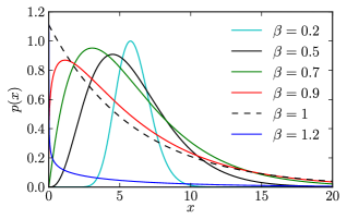
The radial distribution of BLR emission density is described by a shifted gamma distribution. The gamma distribution for a positive variable is usually written
| (8) |
where is the shape parameter and is a scale parameter. Our radial distribution is based on a shifted gamma distribution where the lower limit is instead of zero. Rather than parameterizing the distribution by , whose interpretations are not straightforward (making priors difficult to assign), we use a different parameterisation in terms of three parameters , defined as follows.
| (9) | |||||
| (10) | |||||
| (11) |
The parameter is the mean value of the shifted gamma distribution, is the standard deviation of the gamma distribution in units of the mean when , and is the fraction of from the origin at which the gamma distribution begins (i.e. is measured in units of ). For arbitrary , the standard deviation of the shifted gamma distribution is:
| (12) |
Finally, we also offset the radial distribution by the Schwarzschild radius, , to provide a hard limit to how close a point particle can be to the black hole. For a black hole, light days, much smaller than the typical size of the BLR, which is on the order of light days.
The three parameters control the radial profile of the particles. To parameterise the actual distances of the particles from the black hole, instead of using the physical distance , we use a variable (one for each particle) with a Gamma prior. Then the actual distance of the particle is computed by:
| (13) |
The reason for parameterizing in terms of rather than is that Metropolis proposals are simpler. For example, a Metropolis move that changes the parameters but leaves fixed will automatically move all of the particles appropriately.
2.4.2 Opening and Inclination Angles
The radial BLR distribution discussed in the previous section is spherically symmetric, however we can break spherical symmetry by introducing a disk opening angle of the BLR. The opening angle is defined as half the angular thickness of the BLR in the angular spherical polar coordinate perpendicular to the plane of the disk. If the BLR is a sphere then the opening angle is , and if the BLR is a thin disk then the opening angle approaches zero. Once spherical symmetry has been broken, it is necessary to consider at what angle an observer will view the BLR. The inclination angle is defined as the angle between a face-on BLR geometry and the observer’s line of sight, so an edge-on disk would have an inclination angle of while a face-on disk would have an inclination angle approaching zero.
To construct a specific BLR geometry, we begin by drawing the radial position for each particle in a flat disk in the - plane with the observer located at the positive end of the -axis. In plane polar coordinates, the radial coordinates of the point particles are calculated using Equation 13, and the angular coordinates are drawn from a uniform distribution between 0 and . We then puff up this flat disk by the opening angle, first by rotating each particle around the -axis by some angle between 0 and the opening angle and then by rotating the particle around the -axis by some angle between 0 and to restore axisymmetry. Next, we rotate all point particles around the -axis by 90 degrees minus the inclination angle so that an inclination angle of zero corresponds to a face-on BLR geometry. All of the angles used in this process are extra model parameters.
2.4.3 Angular BLR Distribution
We can further add asymmetry by controlling the strength of emission from a given particle using three separate effects:
-
1.
The particles are assigned non-uniform weights, depending upon the angle between the observer’s line of sight to the central source and a particle’s line of sight to the central source. The strength of this effect is controlled by a parameter .
-
2.
The parameter controls the extent to which the emission is concentrated near the outer edges of the BLR disk at the opening angle.
-
3.
The parameter determines the transparency of the plane of the BLR disk.
The first effect represents anisotropic emission from the point particles. We use first order spherical harmonics to define a weight, , for each particle that ranges from 0 to 1 and determines what fraction of the continuum flux is reemitted as line flux in the direction of the observer:
| (14) |
The one free parameter is , which ranges from to . Negative values of correspond to preferential emission from the far side of the BLR from the observer and positive values correspond to preferential emission from the near side of the BLR. Preferential emission from the far side of the BLR could be physically caused by BLR gas only re-emitting continuum emission back towards the central source due to self-shielding, while preferential emission from the near side of the BLR could be physically caused by the closer BLR gas blocking gas farther away. The angle is defined to be the angle between the observer’s line of sight to the central source and the particle’s line of sight to the central source. For and a model where the BLR is made up of spherical balls of gas, this model is equivalent to considering broad line emission from the area of the spheres illuminated by the central source as viewed by the observer, like lunar phases.
The second effect is parameterized by and controls the extent to which BLR emission is concentrated near the outer faces of a disk. This could arise for example if the parts of the BLR closer to the plane of the accretion disk are optically thick. The parameter controls preferential emission from the outer faces of the BLR disk by affecting how much the particle positions are moved from an initial flat disk to between zero and the opening angle of a thick disk. The angle for a particle’s displacement from a flat to thick disk is given by:
| (15) |
where is the opening angle and is a random number drawn uniformly between 0 and 1. Larger values of lead to values closer to , so using with between 1 and 5 concentrates more particles close to the opening angle for .
The third effect represents the possibility for an obscuring medium in the plane of the BLR to partly or completely obscure broad line emission from the back side of the BLR and is parameterized by . Unlike the first effect that depends upon the inclination angle at which an observer views the BLR, is roughly defined as the fraction of particles on the far side of the BLR midplane. In the limit of , the entire back half of the BLR is obscured, and the BLR geometry could range from half a disk or sphere when to a single cone when . In the limit of , the back half of the BLR is not obscured. Since it is computationally inefficient to throw out particles on the back side of the BLR, we actually just invert their position with respect to the plane of BLR when , making the true definition of be the fraction of particles in the back side of the BLR that have not been moved to the front side.
2.5 Dynamics Models
In order to make a model spectrum from our geometry of the BLR we must also assign velocities to the particles. We consider three different kinematic components, including bound elliptical orbits and a combination of both bound and unbound inflow or outflow.
2.5.1 Elliptical Orbits
Consider a particle orbiting a point mass at a distance with velocity , where is the radial velocity and is the tangential velocity in the plane of the orbit and perpendicular to . The tangential velocity in terms of the angular momentum per unit mass of the particle is given by , and the radial velocity can be obtained by considering the energy per unit mass of the particle:
| (16) |
Solving for we obtain:
| (17) |
For circular orbits, we have the additional constraint that so that the centripetal force of circular motion must equal the gravitational force, giving or . Thus, the circular orbit solutions are two special points in the plane at .
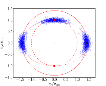
We consider generalizations of circular orbits to elliptical orbits by considering distributions in and centered around the circular orbit solutions. Such a model allows us to recover circular orbits when the distributions are narrow, but also allows for highly elliptical orbits when the distributions are on the order of . We draw the velocities of the particles from the ellipse in the and plane that has semi-minor axis at and semi-major axis equal to the escape velocity at , as shown in Figure 2. The reason for drawing velocities from around this ellipse instead of a circle with radius is that the parameter space naturally includes the points at that correspond to the radial outflowing and inflowing escape velocities. We will discuss these inflowing and outflowing velocity solutions in more detail in Section 2.5.2. Since reverberation mapping measurements cannot distinguish between rotations of the BLR around the line of sight axis, it is only necessary to define the positive side of the plane. The radial and tangential velocities are thus drawn from Gaussian distributions centered at with standard deviations given by and , where is the radial coordinate in the plane and is the angular coordinate. Circular orbits are recovered when and , whereas highly elliptical orbits approaching the escape velocity are obtained when and , the upper limits of their priors.
2.5.2 Inflow and Outflow
In order to include the possibility of substantial unbound outflowing or inflowing gas in the BLR, we allow a variable fraction of the point particles to have elliptical, inflowing, and outflowing orbits. Since we do not expect to find both inflowing and outflowing gas in the BLR in the same spatial location, especially at the velocities assumed by our model, we only allow for inflowing or outflowing particles in addition to elliptical orbits for a specific instance of our model. The fraction of particles with elliptical orbits is given by , where is thus the fraction of particles in either inflowing or outflowing orbits. Whether the orbits are inflowing or outflowing is given by , where values between 0 and 1 and less than 0.5 denote inflow and values greater than 0.5 denote outflow. Inflowing orbits are obtained around values of while outflowing orbits are obtained around values of .
As for elliptical orbits, we draw the radial and tangential velocities of inflowing or outflowing particles from Gaussian distributions for and , the radial and angular coordinates of the plane. The width of the Gaussian distributions is similarly given by and , where the widths are the same for both inflowing and outflowing orbits. Since the Gaussian distributions are centered on the points , about half of the inflowing and outflowing particles will actually have bound orbits. In order to allow for completely bound inflowing and outflowing trajectories, we also allow the distributions centered around to be rotated by an angle along the ellipse connecting to the circular orbit velocities . When , the inflowing or outflowing orbits are centered around the escape velocities at , while recovers bound elliptical orbits centered around circular orbits. When , we obtain mostly bound inflowing or outflowing gas.
2.5.3 Macroturbulent Velocities
We also consider macroturbulent velocities of the particles in addition to the velocities from elliptical, inflowing, or outflowing orbits. For each particle, we calculate the magnitude of the turbulent velocity along the observer’s line of sight, given by:
| (18) |
where is a normal distribution centered on zero and with standard deviation . The magnitude of the turbulent velocity is relative to the magnitude of the velocity of the particle’s circular orbit described in Section 2.5.1, given by . We can recover the case with no additional turbulent velocities when . We apply the additional macroturbulent velocity to a point particle first by calculating the elliptical, inflowing, or outflowing velocity and then adding . This model for macroturbulent velocities is similar to the one presented by Goad et al. (2012) for the case of a disk with constant opening angle.
2.5.4 Relativistic Effects
As highlighted in Goad et al. (2012), relativistic effects can have a strong influence on the shape of emission line profiles if the BLR gas is sufficiently close to the black hole. We include two simple relativistic effects in the calculation of particle velocities. The first effect is the full relativistic expression for the doppler shift of the broad emission line due to the line of sight velocity of the emitting BLR gas. The second relativistic effect is that of gravitational redshift, which is caused by a photon being emitted from deeper in a gravitational potential well than the observer of the photon. The wavelength shift caused by gravitational redshift depends upon the ratio of the Schwarzschild radius, , to the radial distance of the emitting source. Together, the full relativistic expression for doppler shift and the expression for gravitational redshift act to shift the emitted wavelength of line emission from a particle to the observed wavelength given by:
| (19) |
where the particle has velocity and radial distance from the black hole . Since we compare our model broad emission line spectra to the data in wavelength space, we can include the relativistic doppler shift and gravitational redshift in the simulated data by converting the simulated data from velocity to wavelength space using Equation 19.
2.5.5 Narrow Line Emission
In addition to a model of the broad emission line, we must also consider the superimposed narrow emission line from the narrow line region (NLR). Since the NLR is farther from the black hole, the narrow emission line is not expected to reverberate on timescales as short as those for the BLR (e.g. Peterson et al., 2013). We therefore assume that the narrow emission line flux is constant over the duration of a reverberation mapping dataset. We model the narrow emission line component using a Gaussian with line dispersion given by another more isolated narrow emission line profile. For example, to model the narrow component of the H emission line we use the line dispersion of the narrow [O iii] emission line, just red-ward of H. Since the width of [O iii] in a given reverberation mapping dataset is due to both intrinsic line width and instrumental resolution, we use measurements of the intrinsic line width to calculate the instrumental resolution, which is needed to smooth the model spectra. Differences in observing conditions can also change the instrumental resolution as a function of time, so we calculate the line dispersion of the narrow [O iii] line for each spectrum individually and include the measurements of the line dispersion as free parameters with Gaussian priors given by the line width measurement uncertainties. The intrinsic narrow line width of [O iii] is also treated as a free parameter with a Gaussian prior given by the line width measurement uncertainties. For objects where the NLR is not resolved and thus there is no intrinsic line width to the narrow line profile, the width of the narrow emission line directly gives a measurement of the instrumental resolution. Since subtracting narrow emission lines from broad emission lines can introduce significant uncertainty into the spectrum, we model spectra that have not had the narrow emission line subtracted and we include the total flux of the narrow line as an additional free parameter to be constrained by the data.
2.6 Exploring Parameter Space
| Parameter | Definition | Prior |
|---|---|---|
| Mean radius of the BLR radial profile Eq. 9 | LogUniform | |
| Unit standard deviation of BLR radial profile Eq. 10 | Uniform | |
| Beginning radius in units of of BLR radial profile Eq. 11 | Uniform | |
| Inclination angle § 2.4.2 | Uniform() | |
| Opening angle § 2.4.2 | Uniform | |
| Cosine illumination function parameter Eq. 14 | Uniform | |
| Disk edge illumination parameter Eq. 15 | Uniform | |
| Plane transparency fraction § 2.4.3 | Uniform | |
| Black hole mass Eq. 16 | LogUniform | |
| Fraction of elliptical orbits § 2.5.2 | Uniform | |
| Flag determining inflowing or outflowing orbits § 2.5.2 | Uniform | |
| Radial standard deviation around circular orbits § 2.5.1 | LogUniform | |
| Angular standard deviation around circular orbits § 2.5.1 | LogUniform | |
| Radial standard deviation around radial orbits § 2.5.2 | LogUniform | |
| Angular standard deviation around radial orbits § 2.5.2 | LogUniform | |
| Standard deviation of turbulent velocities § 2.5.3 | LogUniform | |
| Angle in the plane § 2.5.2 | Uniform |
Equation numbers refer to the first equation in which the parameter is used and section numbers refer to those subsections where the parameter is defined. is the time span between the first and last data point in the reverberation mapping dataset. The prior is designated by the scale in which a parameter is sampled uniformly and by the range (minimum value, maximum value). Uniform denotes a uniform prior distribution between 0 and 1. LogUniform denotes a uniform prior for the log of the parameter, or alternatively, a prior density , between the parameter values and . A log-uniform prior is used for positive parameters whose order of magnitude is unknown.
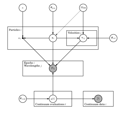
Once our model of the BLR has been defined, we can explore this high-dimensional parameter space to constrain which parameter values best fit a specific reverberation mapping dataset by measuring the posterior PDFs and correlations between parameters. The full list of all parameters in our BLR model is given in Table 1 along with all of the random numbers used to assign the point particle positions and velocities in Section 2. A probalistic graphical model (PGM) of the interdependence of the parameters is shown in Figure 3. One way to interpret Figure 3 is as a recipe for making simulated reverberation mapping data:
-
1.
Generate a model continuum light curve using Gaussian processes and then
-
2.
sample it to create a realistic continuum light curve.
-
3.
Use BLR geometry and dynamics parameters to generate the positions and velocities of all the particles in the BLR.
-
4.
Finally, use those positions and velocities along with the model continuum light curve to make a simulated time series of broad emission line spectra or integrated broad line fluxes.
As described in Section 2.2, we can explore high-dimensional parameter spaces using an MCMC algorithm. We use the diffusive nested sampling code DNest (Brewer et al., 2011b) due to its ability to explore correlations between parameters efficiently in high dimensional spaces, and because it calculates the Bayesian evidence and thus allows for model selection. DNest works by using multiple walkers to explore parameter space, starting from the prior and gradually adding hard likelihood constraints.
One of the inherent difficulties of fitting real data with a simplified model is that the model is unlikely to match the data perfectly, especially if the error bars on the data are very small. In practice, one often obtains unrealistically precise inferences of the model parameters because the model contains simplifications. However we still expect the model to capture the main features of the structure of the BLR. We account for the systematic uncertainty from using a simple model by inflating the errorbars of the data until only the macroscopic fluctuations in the data are fit by the model. Since we use a Gaussian likelihood function, as discussed in Section 2.2, we can rephrase the inflation of errorbars as an increased weighting of the prior probability compared to the likelihood when calculating the posterior probability. The weighting term is called a “temperature” , such that and hence the inflated errorbars are larger than the original errorbars for a Gaussian likelihood function. Generally higher quality datasets require larger values of . Another advantage of using nested sampling for the computation is that we can vary the temperature and check the sensitivity of the results without having to repeat the MCMC run.
2.7 Limitations of the Model and Future Improvements
Finally, we discuss some of the limitations of our model of the BLR and discuss improvements to be made in the future. One of the main limitations of our model is the simplified dynamics of the point particles. We ignore the effects of radiation pressure, a force that has a dependence like gravity, making it difficult to disentangle from the black hole mass. Unfortunately, this degeneracy of radiation pressure with black hole mass means that black hole masses could be significantly underestimated, and that the degeneracy can only be broken by including external information about the BLR gas density in the model (Marconi et al., 2008, 2009; Netzer, 2009; Netzer & Marziani, 2010). We also ignore the self-gravity and viscosity of the BLR gas and any interaction it has with the gas in the accretion disk. Finally, we assume that the gas in elliptical orbits is the same gas that could be inflowing or outflowing, when in reality the BLR could have multiple components with different geometries and dynamics.
Another limitation to our model of the BLR is the simplified treatment of radiative transfer, both for the ionizing and broad line photons. We ignore any asymmetry of the ionizing photons except for an optional preference for photons away from the BLR midplane. We also ignore detailed radiative transfer of line photons within the BLR gas, both locally and globally. While we have included two additional obscuration effects in this new version of the BLR model, transparency of the disk midplane to line photons () and asymmetry of the ionizing photons away from the disk midplane (), these are simplifications of what is most likely an inherently complicated problem.
Some of these limitations can be at least partially solved in future models of the BLR. For example, CLOUDY models constrain the direction in which line photons are emitted from individual clouds of BLR gas, as well as the emissivity and responsivity of line emission as a function of radius (e.g. Ferland et al., 1998, 2013). Using a table of pre-computed values from CLOUDY would not only provide a more physically-detailed local opacity to our model, but would also constrain the radial distribution of broad line emitting gas. By modeling the BLR using multiple broad emission lines simultaneously, we can also start to place constraints on the underlying distribution of gas density.
Recently Li et al. (2013) developed an independent code to model reverberation mapping data using a geometry model of the BLR based on the model of Pancoast et al. (2011). They include additional flexibility in their model by allowing for non-linear response of the broad emission lines to incident continuum radiation. While the average emission line response of their sample is close to linear, they find that individual AGNs can have non-linear response, suggesting that this effect may be important to include in future implementations of our modeling code.
Another improvement that could be made to our model is better treatment of the dynamics. One option could be to include separate geometries for each dynamical component, for example a thin disk of gas in elliptical orbits with a cone of outflowing gas. We could also improve our treatment of outflows to include the detailed dynamics found in simulations of disk winds or complex models of outflows. For example, instead of assuming that outflowing gas has mainly radial trajectories at or near the escape velocity of its present position, we could consider the more complicated case where the gas is accelerated to velocities on the order of the escape velocity and where the escape velocity is defined at an initial wind launching radius instead of the current position of the gas (e.g. Castor et al., 1975; Proga, 1999).
Finally, breathing of the BLR may play an important role in determining the response of emission line flux as a function of time (see Korista & Goad, 2004, and references therein). Breathing of the BLR is where BLR emission comes from gas farther from or closer to the central engine based on increases or decreases in the ionizing luminosity, respectively. If the mean radius of the BLR changes substantially over the course of a reverberation mapping campaign, then this could have a noticeable effect on the measured time lag and the results from direct modeling analysis.
3 Tests with Simulated Data and Arp 151
We demonstrate the capabilities of our improved model of the BLR and direct modeling code by recovering the model parameters for two simulated reverberation mapping datasets. By modeling the time series of emission line profiles using a geometry and dynamical model of the BLR as well as modeling the integrated emission line light curve using a geometry model of the BLR, we illustrate the benefits of a full spectroscopic dataset.
3.1 The simulated datasets
| Geometry Model | Simulated | Simulated | Simulated | Simulated |
| Parameter | Data 1 (True) | Data 1 (Inferred) | Data 2 (True) | Data 2 (Inferred) |
| (light days) | ||||
| (light days) | ||||
| (light days) | ||||
| (days) | ||||
| (degrees) | ||||
| (degrees) | ||||
| Dynamical Model | Simulated | Simulated | Simulated | Simulated |
| Parameter | Data 1 (True) | Data 1 (Inferred) | Data 2 (True) | Data 2 (Inferred) |
| – | ||||
| (degrees) | – | |||
The columns with (True) give the true parameter values for the simulated datasets and the columns with (Inferred) give the inferred parameter values and their uncertainties. True parameter values with – are unimportant for that specific simulated dataset.
In order to generate realistic simulated reverberation mapping datasets, we use the LAMP 2008 dataset of H emission for Arp 151 (Walsh et al., 2009; Bentz et al., 2009) to determine the sampling cadence, flux errors, instrumental smoothing, and approximate scale of the BLR. The Arp 151 dataset includes a B-band continuum light curve and a time series of H emission line profiles, where the broad and narrow H flux is isolated from the spectrum using spectral decomposition techniques as described by Park et al. (2012b). As described in Section 2.6, the simulated datasets are created by first generating a model of the Arp 151 continuum light curve using Gaussian processes and sampling that model continuum light curve with the same cadence as for Arp 151. We then add Gaussian noise to the continuum light curve using the error vector of the Arp 151 light curve. Next we set fixed the BLR geometry and dynamics model parameters to the values found in Table 2 and sample the H emission line profile at the times given by the Arp 151 spectral dataset. Finally, we add Gaussian noise to the model spectra based on the spectral errors in the Arp 151 dataset. In order to account for the fact that real reverberation mapping datasets are likely more complicated than our model of the BLR assumes, we inflate the spectral errors and added Gaussian noise on the simulated dataset by a factor of three compared to the Arp 151 dataset, to obtain more realistic uncertainties on the inferred model parameters. To reduce numerical noise in the simulated spectra to less than the uncertainty in the spectral fluxes, we use 2000 particles and assign each one ten independent velocity values. The width of the narrow line component of H is modeled using the line dispersion of the narrow [O iii] emission line from the Arp 151 dataset, calculated for each epoch of spectroscopy. The instrumental resolution is then measured by comparing the measured line dispersion for [O iii] with its intrinsic line width as calculated by Whittle (1992).
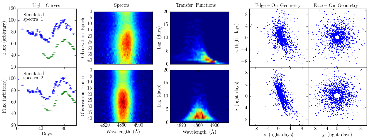
The simulated datasets are based on the geometry and dynamics inferred for the LAMP 2008 dataset in paper II as shown in Table 2, with small mean radii for the BLR of light days, close to exponential radial profiles with , substantial width to the BLR of light days, thick disks with opening angles of degrees, close to face-on inclination angles of 20 degrees, preferential emission from the far side of the BLR () and the edges of the disk (), and mostly opaque mid-planes (). The black hole masses are also chosen to be similar to the LAMP 2008 sample with and each of the simulated datasets is dominated by either elliptical orbits or inflowing orbits. The differences between the simulated datasets can also be easily seen in Figure 4, which shows not only the continuum, line, and spectral timeseries, but also the transfer functions and geometries of the BLR. The simulated spectral datasets consist of the following:
-
1.
A thick, wide disk with an exponential profile and dynamics dominated by inflowing orbits.
-
2.
A thinner, narrower disk, with a radial profile between a Gaussian and exponential and dynamics dominated by elliptical orbits.
The continuum light curve interpolation using Gaussian processes is also held constant for all three simulated datasets, although the random noise added to each realistically sampled continuum light curve is different.
While not an issue for simulated emission line profiles, real reverberation mapping data must contend with ambiguity in multiple spectral components overlying the broad emission line profile. For example, with H we not only have possible overlap of the red wing with the narrow [O iii] emission lines and the blue wing with He ii, but there may also be substantial overlap with Fe ii broad line emission. Blending between multiple broad components is especially important to disentangle because the different broad emission lines will be generated in BLR gas at different radii from the black hole and blending could confuse the dynamical modeling results. In order to isolate any single broad emission line profile, it is necessary to apply a method of spectral decomposition that will remove most of the ambiguity in overlapping spectral components.
3.2 Recovery of model parameters: spectral datasets
As a first test of our direct modeling code and BLR model, we attempt to recover the true parameter values of the two simulated spectral datasets described in Section 3.1. We assume the same instrumental resolutions as a function of time that are used to generate the simulated datasets and use 2000 particles and assign ten independent velocities to each one. Since we add Gaussian noise to the simulated datasets, we do not expect to recover every parameter of the BLR exactly. In addition, certain BLR geometries and dynamics make it difficult to constrain certain parameters. For example, when the majority of particles are in elliptical orbits, the fraction of particles in inflowing or outflowing orbits may not be well constrained. Or, a nearly face-on very thin disk will make it difficult to constrain the parameters , , and since these parameters affect the relative line emission throughout the height of the very thin disk in this case.
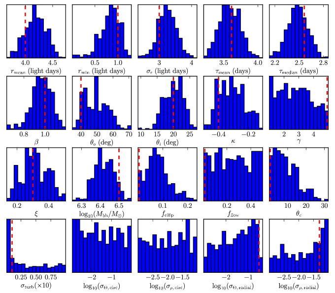
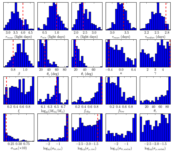
The inferred posterior PDFs for the BLR geometry and dynamics model parameters are shown in Figures 5 and 6 for simulated datasets 1 and 2, respectively. The true parameter values for the simulated datasets are shown by vertical red dashed lines for comparison, and in the cases where the true parameter value does not matter (e.g. when the dynamics are entirely dominated by elliptical orbits so there is no true value of ) no red line is given. Overall, the modeling code is able to recover the true parameter values to within reasonable uncertainties, as listed in Table 2. Specifically, we constrain the mean radius of the BLR to within 0.5 light days uncertainty, the mean time lag to within 0.2 days uncertainty, and the inclination and opening angles to within degrees. The geometry parameters that add asymmetry to the BLR are more difficult to constrain, with and well constrained for simulated dataset 1 while neither , , nor are well-determined for simulated dataset 2.
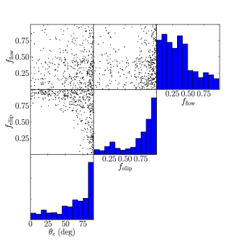
We also constrain to dex uncertainty, where the variation comes mainly from larger correlated uncertainties with the inclination and opening angles for simulated dataset 2. The dynamics are also well-recovered for both simulated datasets, with a clear preference for inflow in simulated dataset 1 and for elliptical orbits centered around the circular orbit values in simulated dataset 2. A clearer picture of the preference for elliptical orbits for simulated dataset 2 can be seen in Figure 7, which shows the correlations between , , and . Specifically, for values of approaching 90 degrees, the distribution of inflowing or outflowing orbits becomes identical to the distribution for elliptical orbits centered around the circular orbit value in the plane. This means that when degrees, although and are mostly unconstrained, the velocity distribution for the particles is very similar to that of .
In general, these two simulated spectral datasets show that we can expect to obtain substantial constraints on the geometry and dynamics of the BLR for reverberation mapping datasets similar in quality to LAMP 2008. The potential constraints on the black hole mass are also promising, although they depend upon the geometry of the BLR, specifically the precision with which we can measure the inclination and opening angles.
3.3 Recovery of model parameters: integrated line datasets
For those cases where a full spectroscopic reverberation mapping dataset is not available, we can apply a geometry-only model of the BLR and reproduce integrated emission line flux light curves. We test whether this approach provides constraints on the geometry of the BLR that are comparable to the full geometry plus dynamical modeling problem using the simulated datasets described in Section 3.1 and shown in the left panel of Figure 4.
We find that the mean time lag and mean radius are well constrained with geometry-only modeling. The mean and median time lag inferred for each simulated dataset are given in Table 3, along with the true mean and median lag values and the value measured by CCF analysis. The inferred mean time lag is not only accurate, but the inferred uncertainty in the mean time lag through geometry-only modeling of days is almost half as large as for the CCF time lag. This shows that geometry-only modeling is a promising tool for measuring time lags. The mean radius is inferred with slightly larger uncertainties to be light days for simulated dataset 1 and for simulated dataset 2, while the true mean radius is light days.
Unfortunately the other geometry model parameters are not as well constrained. The parameters and are completely unconstrained for both of the simulated datasets, and , , , , and are mostly unconstrained. Generally there is a slight preference for a specific value of , , , , and , but none or almost none of the parameter space is ruled out. These results for geometry-only modeling suggest that a full spectroscopic reverberation mapping dataset is needed to constrain the geometry of the BLR, since otherwise there are too many degeneracies between model parameters to infer anything other than the mean time lag and mean radius consistently.
3.4 Comparison with JAVELIN
| Lag (days) | Sim Data 1 | Sim Data 2 |
|---|---|---|
| True mean lag | ||
| True median lag | ||
and are the mean and median time lags inferred from BLR geometry modeling, is the time lag measured by JAVELIN, and is the center-of-mass lag measured from the CCF.
Recently another method has been developed for measuring the time lag in reverberation mapping data using integrated emission line light curves by Zu et al. (2011). This method has been implemented in an open-source code called JAVELIN written in Python.222Download JAVELIN here: https://bitbucket.org/nye17/javelin JAVELIN works by using a top-hat transfer function with two parameters, a mean lag and a width of the top hat. The continuum light curve in JAVELN is interpolated using a CAR(1) model, which is equivalent to the continuum model implemented here. The parameter space of the continuum light curve and transfer function models is sampled using MCMC, providing posterior PDFs for the model parameter values.
We can compare recovery of the time lag using BLR geometry modeling of integrated emission line light curves to the results from JAVELIN. For simulated dataset 1, we measure a mean lag of days and a mean width of the top-hat transfer function of days using JAVELIN. This can be compared to the true mean lag of 3.62 days and the true median lag of 2.56 days for simulated dataset 1 to see that the mean lag measured by JAVELIN is between the true mean and median lags. For simulated dataset 2, we measure days and days. Again, the mean lag measured by JAVELIN is between the true mean lag of 3.39 days and the true median time lag of 2.77 days, although closer to the mean lag. The tendency for the time lag measured by JAVELIN to fall closer to the true mean or median lag is due to the shape of the transfer function; in very asymmetric transfer functions, the mean and median time lag are increasingly discrepant, with JAVELIN more sensitive to the true median time lag for very asymmetric transfer functions.
While the tendency of JAVELIN to measure a time lag ranging between the true mean and median time lags may appear to complicate its interpretation, an uncertainty of day from the difference between the true mean and median lags is comparable to the uncertainty introduced by additional assumptions, as discussed in Section 4, when using time lag measurements to estimate the mean radius of the BLR or to measure the black hole mass. These comparisons suggests that JAVELIN is a excellent resource for measuring the time lag even if the JAVELIN lag uncertainties do not reflect the uncertainty introduced by asymmetric transfer functions. However, to constrain more than the time lag, more flexible modeling of the transfer function must be done.
In comparison, the CCF lag measurements for the two simulated datasets agree with the true mean lag values due to larger uncertainties. The CCF lag measurements do not agree more closely with the true median lag values than with the true mean lag values for more asymmetric transfer functions, as for JAVELIN lags. The quoted error bars on the CCF lag values, , in Table 3 are calculated by drawing a random subset of the line and continuum light curves points, with the same number of random draws as the original light curves. For points in the light curves that are drawn times, the flux error is reduced by . Finally, the randomly drawn light curve fluxes are modified by adding random Gaussian noise given by the flux errors. This is similar to the “flux randomization”/“random subset selection” (FR/RSS) approach described in Peterson et al. (1998) except the FR/RSS approach throws out any redundant points in the light curve instead of reducing the flux errors by , resulting in slightly larger uncertainties in the CCF lag. The CCF time lag is measured for 1000 iterations of this sequence and we quote the median and 68% confidence intervals of the CCF time lag distributions. For the two simulated datasets tested here with data quality comparable to the LAMP 2008 dataset for Arp 151 (Bentz et al., 2009), the error bars are days, or % the value of . This comparison suggests that while CCF analysis may not give the most precise measurement of the mean or median time lag, the CCF lag uncertainties likely include much of the systematic uncertainties from an unknown transfer function.
Finally, we also consider the effects of detrending the light curves before calculating the CCF lag. Detrending can improve the shape of the CCF when there are strong long-term trends that can be removed by subtracting a linear fit to the light curves (Welsh, 1999). Since our simulated data do not contain strong long-term trends, detrending the light curves should have minimal impact on the measured CCF lags. We confirm this by subtracting a linear fit to the simulated continuum light curves from both the continuum and line light curves. Due to the difference in length between the continuum and line light curves, fitting the continuum and line light curves with linear fits separately destroys the correlation between the light curves. When we use a linear fit to the continuum light curve to detrend both light curves we obtain CCF lag measurements for simulated dataset 1 of days and for simulated dataset 2 of days, which agree to within the uncertainties with the un-detrended CCF lag values.
3.5 Dynamical modeling without a full spectral dataset
As shown in Section 3.3, a spectroscopic dataset offers substantially more information about the BLR for direct modeling. Here we explore an intermediate case, where the available data consist of the usual continuum light curve, an integrated emission line light curve, and a mean spectrum. Since the mean spectrum contains some information about the kinematics of the BLR, we can model this dataset using the fully dynamical model of the BLR. However, with only the mean spectrum, this dataset cannot constrain the time lag as a function of velocity or wavelength, as possible for a full spectroscopic dataset.
In order to provide a test of this intermediate dataset case that is as realistic as possible, we use the LAMP 2008 dataset for Arp 151. A description of the dataset can be found in paper II. In the analysis of this test, we focus on the differences in inferred parameter values between this test and the full dynamical modeling results presented in paper II. In general, the modeling results for the full spectroscopic dataset and for the intermediate dataset are fully consistent, but the uncertainty on the inferred model parameter values is much larger for the intermediate dataset. For example, the black hole mass is inferred to have a posterior PDF with a long tail at high masses, giving compared to the value from Paper II of . Similarly, the uncertainty in , , and is larger by at least a factor of 3, the uncertainty in is larger by at least a factor of two, and is completely undetermined for the intermediate dataset. The two marginally consistent results are the mean radius and mean lag, which are both substantially larger for the intermediate dataset and have uncertainties at least 10 times larger than for the full spectroscopic dataset. This is due to a preference for , corresponding to heavy-tailed radial distributions where the median radius and median lag are more consistent measurements of the characteristic size of the BLR. Overall, this test suggests that considerable information about the BLR can be inferred from the mean line profile, but the constraints on BLR geometry and dynamics parameters are significantly better when the full spectroscopic dataset is used. Finally, while this intermediate dataset allows for measurement of the black hole mass, it cannot be constrained to less than the dex scatter in the factor due to a tail in the posterior PDF at high masses.
4 Comparison with cross-correlation analysis
We can compare the results of direct modeling to the standard reverberation mapping analysis of using the cross-correlation function (CCF) to measure time lags and the dispersion or FWHM of the broad emission line to measure a characteristic velocity of the BLR. In addition to providing a sanity check on our direct modeling results, such a comparison allows us to explore some of the uncertainties involved in standard reverberation mapping analysis. First, we consider the time lag traditionally measured using the CCF, how it compares to a measurement of the mean radius and how sampling of the line light curve and variability of the continuum light curve affect its measurement. Second, we consider the combination of the CCF lag with measurements of the emission line width to explore the uncertainty in black hole masses measured using the virial product.
4.1 Comparing the time lag and mean radius
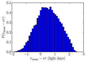
One of the main assumptions in the traditional analysis is that the time lag measured from CCF analysis is related to some characteristic radius of the BLR. We explore the validity of this assumption by comparing the mean radius and the mean time lag in our geometry model of the BLR. We hold the mean radius fixed at light days and allow the other geometry model parameter values to sample their priors as listed in Table 1, with the exception of the inclination angle, which we constrain to vary between zero (face-on) and 45 degrees. The results of this comparison are shown in Figure 8 for 200,000 samples. The difference between the mean radius, , and the mean lag, , is generally greater than one, meaning that the mean lag (in days) is usually shorter than the mean radius (in light days). This is due to the geometry parameter that allows the midplane of the BLR to be transparent or opaque, since a BLR midplane that is not transparent will result in fewer particles with longer lags and hence a tendency for the mean lag to be smaller than the mean radius. The mean of is 0.53 light days and the standard deviation of the distribution is 0.80 light days. This suggests that the uncertainty in using the time lag as a measurement of the mean radius is relatively small, on the order of the CCF time lag uncertainty typically quoted for high-quality reverberation mapping data of day.
4.2 The effects of line light curve sampling
| Mock | |||||||
|---|---|---|---|---|---|---|---|
| Line | (days) | (deg) | (deg) | ||||
| 1 | 3.69 | 10 | 25 | -0.25 | 1.0 | 0.2 | 0.5 |
| 2 | 3.77 | 10 | 25 | 0.5 | 0.11 | 0.5 | 1 |
| 3 | 4.01 | 10 | 90 | 0.0 | 0.11 | 0.99 | 1 |
| 4 | 5.34 | 10 | 90 | -0.5 | 0.11 | 0.99 | 1 |
| 5 | 4.00 | 0 | 0.5 | 0.0 | 0.11 | 0.99 | 1 |
All simulated datasets were created with a mean radius, , of 4 light days and with .

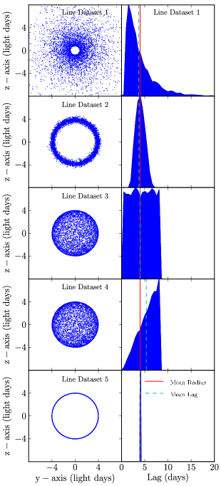
Next we explore the dependence of the measured CCF lag on the geometry of the BLR and on the sampling characteristics of the emission line light curve. We focus on four very simple BLR geometries and one more realistic one, as shown in Figure 10, including
-
1.
A nearly face-on wide disk with preferential emission from the far side and a disk midplane that is more than half opaque.
-
2.
A nearly face-on ring with preferential emission from the near side.
-
3.
A spherical shell (making a top-hat transfer function).
-
4.
A spherical shell with preferential emission from the far side.
-
5.
A perfectly face-on thin ring (making a -function transfer function).
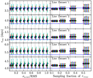
We use these five geometries of the BLR to create simulated emission line light curves, as shown in Figure 9 using the same input continuum light curve and with very fine sampling of 0.1 days for both the line and continuum light curves. The geometry model parameter values are given in Table 4. In order to test how the quality of integrated emission line light curves affects measurement of the CCF lag, we degraded the quality of the simulated data by adding random Gaussian noise to the line light curve and by reducing the sampling cadence. For each simulated dataset degraded by adding of random Gaussian noise, by sampling the line light curve at some fraction of the true mean radius of the BLR, and by losing a fraction of that sampled line light curve to weather, we computed the CCF lags and for 1000 realizations of assigning the random noise and losing a fraction of the light curve to weather. The simulated line light curves were degraded by:
-
1.
Reducing the sampling cadence to 1/10, 1/5, 1/3, or 1/2 of the true mean radius value of the geometry model of 4 light days. This means that the highest cadence is about half a day.
-
2.
Adding random Gaussian noise, , at the level of 0.05, 0.1, 0.2, 0.3, 0.4, 0.5, 0.6, 0.7, 0.8, 0.9, or 1.0 times the RMS variability of the simulated line light curve.
-
3.
Including only a fraction of the total number of line light curve data points randomly from the light curve to simulate observations lost to weather. The fractions are 1, 3/4, 2/3, and 1/2.
Some illustrative results of this comparison are shown in Figure 11, with the lefthand column showing the CCF lag versus the ratio of over the RMS variability and with the righthand column showing the CCF lag versus the cadence as a sampling fraction of . Figure 11 shows the results for when 3/4 of the line light curve is not lost to weather. The trend continues for larger fractions of the light curve lost to weather: the uncertainties on the measured CCF lag increase while the mean lag measurement stays the same. For the case where no observations are lost to weather, the error bars become comparable to the size of the points in Figure 11. Overall, these results suggest that for different geometries of the BLR can be offset from the true lag value by as much as a quarter of a light day (for a true mean lag of light days, see Table 4 for the exact values), which is well within typical uncertainties on CCF time lags quoted in the literature. For light curves with larger flux errors and lower cadence, this offset is easily within the error bars. In addition to a possible offset from the true lag values, these results show the importance of sampling the light curve at smaller fractions of the mean lag, even when the signal to noise quality of the light curve is high. As the fraction of the light curve lost to weather increases, this effect becomes more important. Detrending of the simulated light curves does not change these results.
4.3 The effects of continuum variability
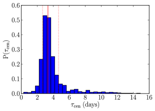
In addition to light curve sampling effects, there is also the possibility that variability features in the AGN continuum light curve could affect measurement of CCF lags. We explore this source of uncertainty by generating 1000 random realizations of AGN continuum light curves, keeping the continuum hyper-parameters fixed to values similar to those inferred for Arp 151 and the BLR geometry model fixed to the values for simulated integrated line dataset 1 given in Table 4. Given each realization of the AGN continuum light curve and the fixed BLR geometry model, we generate an integrated emission line light curve. We use the sampling cadence of the LAMP 2008 dataset for Arp 151, described in Section 3.1, for each realization of the continuum and line light curves. We then calculate the CCF center-of-mass lag for each of the 1000 realizations, obtaining successful CCF lag measurements for over 90% of the random continuum realizations.
The results are shown in Figure 12 as a histogram of values, where we have truncated the histogram to between zero and fifteen days for clarity. The median and 68% confidence interval for all measurements of is days, and considering only values of between zero and fifteen days reduces the uncertainties by less than 0.1 days. Detrending of the simulated light curves results in a similar median value for of days. These inferred median values for agree to within the uncertainties with each other and the true value of the mean lag of days. This test demonstrates that the main consequence of continuum variability is to add additional scatter to measurements of on the order of day, without shifting the median measurement of away from the true value.
4.4 Comparing the black hole mass and virial product
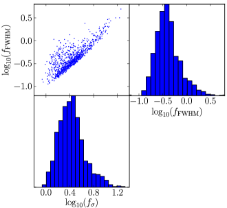
Other than the mean lag from CCF analysis, the black hole mass measured from the virial product is the key measurement of reverberation mapping studies. However the use of the virial product, , to measure black hole mass involves making many assumptions, including that the mean lag is a good measure of the physical scale of the BLR and that the width of the broad emission line is a good measure of the velocity field of the BLR. We attempt to quantify the uncertainty introduced by these assumptions by calculating the virial product from instances of our geometry and dynamics BLR model. We hold the black hole mass fixed at and the mean radius fixed at light days while allowing all other geometry and dynamics model parameters to vary within their prior bounds, except for the inclination angle, which is limited to within zero (face-on) and 45 degrees. For each sample of a BLR model, we calculate the CCF lag , the line dispersion of the RMS emission line profile, and the full width at half maximum (FWHM) of the mean line profile. Using these three values we can calculate the virial product either using the line dispersion or FWHM line width measurement. By further dividing the true black hole mass by the virial product we can work in terms of the virial coefficient , where is calculated from the virial product using the line dispersion and is calculated from the virial product using the FWHM.
The results for the comparison of true black hole mass to virial product are shown in Figure 13 for 1000 samples of the BLR model parameters (other than and , which are held fixed). The cadence of the continuum light curve and spectral time series were based on the cadence of the LAMP 2008 dataset for Arp 151, as described by Bentz et al. (2009). The values of and are clearly correlated, but there is significant scatter in the relation. More importantly, the dispersion in the factors is encouragingly small: the mean value of is 0.43, with a standard deviation of 0.22, and the mean value of is with a standard deviation of 0.26, where the dispersion in the factors does not depend on whether the light curves have been detrended. This means that if the BLR is well described by our phenomenological model, we should not be surprised that the relation based on reverberation mapping black hole mass measurements does not have much larger scatter than the canonical dex found for galaxies with dynamical mass measurements.
5 Conclusions
In this paper we present an improved and expanded simply parameterized phenomenological model of the BLR for direct modeling of reverberation mapping data. In addition to describing the model in detail, we test the performance of the direct modeling approach using simulated reverberation mapping datasets with and without full spectral information. We also use this model of the BLR to explore sources of uncertainty in the traditional cross-correlation analysis used to measure time lags in reverberation mapped AGNs as well as sources of uncertainty in traditional measurements of the black hole mass using the virial product. Our main conclusions are as follows:
-
1.
For simulated data with the same properties as the LAMP 2008 spectroscopic dataset for Arp 151, we can recover the black hole mass to within 0.05-0.25 dex uncertainty and distinguish between elliptical orbits and inflow. We recover the mean radius and mean lag with % uncertainties and the opening angle of the disk and inclination angle to within degrees.
-
2.
For the same simulated datasets, but where integrated emission line fluxes are used instead of the full spectroscopic information, we can use a BLR geometry model to constrain the mean radius and mean lag with % uncertainties and obtain only minimal constraints on the geometry of the BLR.
-
3.
Using a combination of an integrated emission line light curve and a mean emission line profile for direct modeling allows for some constraints on the geometry of the BLR, but with greater uncertainty than from using the full spectroscopic dataset. The uncertainty in is also greater compared to using the full spectroscopic dataset.
-
4.
Comparison of BLR geometry modeling results to those from JAVELIN (Zu et al., 2011) and CCF analysis shows that JAVELIN recovers a time lag between the true mean and median lag, while CCF analysis recovers a time lag closer to the true mean lag. While the larger lag uncertainties from CCF analysis may reflect the unknown shape of the transfer function, the lag uncertainties from JAVELIN are smaller than the difference between the true mean and median time lag.
-
5.
By considering the range in possible BLR geometries of our model, we estimate the uncertainty in converting a mean lag into a mean radius to be %.
-
6.
The CCF lag can be offset from the true lag of a BLR model depending on the geometry. Both signal-to-noise of the flux light curve and sampling rate affect the dispersion in how far the CCF lag is relative to the true lag. Gaps in the light curve due to weather also introduce more uncertainty in the CCF lag.
-
7.
For a given BLR geometry, changes in the variability features of the AGN continuum light curve introduces an uncertainty of % into measurements of the CCF lag .
-
8.
By considering the range in possible BLR geometries and dynamics of our model, we estimate the uncertainty in measuring the black hole mass using the virial product to be smaller than the spread in the relation. We find that the standard deviation of is only dex, i.e. smaller than the uncertainty typically quoted for virial mass estimates.
The tests presented here demonstrate the unique capabilities of dynamical modeling of reverberation mapping data to constrain the geometric and kinematic properties of the BLR. While we can use hybrid datasets consisting of integrated line flux measurements and a mean emission line profile, considerably more information is available from modeling the reverberations across the emission line profile. The improvements we have made to this simply parameterized phenomenological model of the BLR have increased the flexibility of the method to fit a wider variety of emission line profiles. Future improvements will add a deeper connection to photoionization physics, relating the distribution of broad line emission to the distribution of underlying gas, and explore the effects of non-gravitational forces, important for inferring the correct black hole mass.
These tests also confirm that the uncertainties inherent in the traditional analysis of measuring lags using the cross-correlation function and black hole masses using the virial product are relatively small, although larger than the formal uncertainties. The simplified problem of modeling integrated emission line light curves using a geometry-only model for the BLR presents an alternative approach for measuring time lags and mean radii of the BLR compared to the traditional analysis. One advantage to measuring time lags and mean radii with geometry modeling of the BLR is that the final uncertainties reflect the unknown underlying transfer function.
Acknowledgements
We would like to thank Aaron Barth, Mike Goad, Keith Horne, Daniel Proga, and Ying Zu for helpful discussions. AP acknowledges support from the NSF through the Graduate Research Fellowship Program. AP, BJB, and TT acknowledge support from the Packard Foundation through a Packard Fellowship to TT and support from the NSF through awards NSF-CAREER-0642621 and NSF-1108835. BJB is partially supported by the Marsden Fund (Royal Society of New Zealand).
Appendix A Comparison of dynamics model to previous work
In previous versions of our geometric and dynamical model of the BLR, we used a less general dynamical model in which point particle velocities were drawn from distributions of energy and angular momentum centered around the circular orbit energy and angular momentum values and (e.g. Pancoast et al., 2011; Brewer et al., 2011a; Pancoast et al., 2012). We can solve for by evaluating Equation 16 when and :
| (20) |
Similarly, we can solve Equation 16 for , setting and plugging in to find an expression for the angular momentum of a particle in a circular orbit:
| (21) |
This previous E/L model incorporated inflow and outflow in the BLR gas through the fraction of elliptical orbits with positive or negative radial velocity component solutions. The inflowing and outflowing gas in the E/L model is thus always bound to the black hole.
For comparison to the current more general dynamical model in Figure 14, we show the distributions of energy and angular momentum in the plane for direct comparison with Figure 2. The radial and tangential velocity distributions for the E/L model are centered around the red dashed ring of radius and constrained to lie within the solid red circle, corresponding to orbits that are bound to the black hole. The velocity at which a particle becomes unbound is given by setting and solving for , which is . Unfortunately, while the distributions of and are centered around their circular orbit values, the chance of having a particle draw a close to circular orbit is vanishingly small, as shown by the lack of points in Figure 14 at . This suggests a better way of including the circular orbit solution: draw point particle velocities directly from distributions in radial and tangential velocity space instead of in and space.
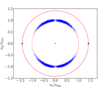
References
- Antonucci (1993) Antonucci, R. 1993, ARA&A, 31, 473
- Barth et al. (2011) Barth, A. J., Nguyen, M. L., Malkan, M. A., et al. 2011, ApJ, 732, 121
- Bentz et al. (2006) Bentz, M. C., Peterson, B. M., Pogge, R. W., Vestergaard, M., & Onken, C. A. 2006, ApJ, 644, 133
- Bentz et al. (2009) Bentz, M. C., Walsh, J. L., Barth, A. J., et al. 2009, ApJ, 705, 199
- Bentz et al. (2013) Bentz, M. C., Denney, K. D., Grier, C. J., et al. 2013, ApJ, 767, 149
- Blandford & McKee (1982) Blandford, R. D., & McKee, C. F. 1982, ApJ, 255, 419
- Brewer et al. (2011a) Brewer, B. J., Pártay, L. B., & Csányi, G. 2011a, Statistics and Computing, 21, 649, astrophysics Source Code Library
- Brewer et al. (2011b) Brewer, B. J., Treu, T., Pancoast, A., et al. 2011b, ApJL, 733, L33
- Castor et al. (1975) Castor, J. I., Abbott, D. C., & Klein, R. I. 1975, ApJ, 195, 157
- Collier et al. (1998) Collier, S. J., Horne, K., Kaspi, S., et al. 1998, ApJ, 500, 162
- Collin et al. (2006) Collin, S., Kawaguchi, T., Peterson, B. M., & Vestergaard, M. 2006, A&A, 456, 75
- Denney et al. (2010) Denney, K. D., Peterson, B. M., Pogge, R. W., et al. 2010, ApJ, 721, 715
- Ferland et al. (1998) Ferland, G. J., Korista, K. T., Verner, D. A., et al. 1998, PASP, 110, 761
- Ferland et al. (2013) Ferland, G. J., Porter, R. L., van Hoof, P. A. M., et al. 2013, RMXAA, 49, 137
- Goad et al. (2012) Goad, M. R., Korista, K. T., & Ruff, A. J. 2012, MNRAS, 426, 3086
- Graham et al. (2011) Graham, A. W., Onken, C. A., Athanassoula, E., & Combes, F. 2011, MNRAS, 412, 2211
- Greene et al. (2010) Greene, J. E., Peng, C. Y., Kim, M., et al. 2010, ApJ, 721, 26
- Grier et al. (2013a) Grier, C. J., Martini, P., Watson, L. C., et al. 2013a, ApJ, 773, 90
- Grier et al. (2013b) Grier, C. J., Peterson, B. M., Horne, K., et al. 2013b, ApJ, 764, 47
- Horne (1994) Horne, K. 1994, in Astronomical Society of the Pacific Conference Series, Vol. 69, Reverberation Mapping of the Broad-Line Region in Active Galactic Nuclei, ed. P. M. Gondhalekar, K. Horne, & B. M. Peterson, 23–25
- Horne et al. (1991) Horne, K., Welsh, W. F., & Peterson, B. M. 1991, ApJL, 367, L5
- Kaspi et al. (2000) Kaspi, S., Smith, P. S., Netzer, H., et al. 2000, ApJ, 533, 631
- Kelly et al. (2009) Kelly, B. C., Bechtold, J., & Siemiginowska, A. 2009, ApJ, 698, 895
- Korista & Goad (2004) Korista, K. T., & Goad, M. R. 2004, ApJ, 606, 749
- Korista et al. (1995) Korista, K. T., Alloin, D., Barr, P., et al. 1995, ApJS, 97, 285
- Kozłowski et al. (2010) Kozłowski, S., Kochanek, C. S., Udalski, A., et al. 2010, ApJ, 708, 927
- Krolik & Done (1995) Krolik, J. H., & Done, C. 1995, ApJ, 440, 166
- Li et al. (2013) Li, Y.-R., Wang, J.-M., Ho, L. C., Du, P., & Bai, J.-M. 2013, ApJ, 779, 110
- Lynden-Bell & Rees (1971) Lynden-Bell, D., & Rees, M. J. 1971, MNRAS, 152, 461
- MacLeod et al. (2010) MacLeod, C. L., Ivezić, Ž., Kochanek, C. S., et al. 2010, ApJ, 721, 1014
- Marconi et al. (2008) Marconi, A., Axon, D. J., Maiolino, R., et al. 2008, ApJ, 678, 693
- Marconi et al. (2009) —. 2009, ApJL, 698, L103
- Morgan et al. (2010) Morgan, C. W., Kochanek, C. S., Morgan, N. D., & Falco, E. E. 2010, ApJ, 712, 1129
- Mushotzky et al. (2011) Mushotzky, R. F., Edelson, R., Baumgartner, W., & Gandhi, P. 2011, ApJL, 743, L12
- Netzer (2009) Netzer, H. 2009, ApJ, 695, 793
- Netzer & Marziani (2010) Netzer, H., & Marziani, P. 2010, ApJ, 724, 318
- Onken et al. (2004) Onken, C. A., Ferrarese, L., Merritt, D., et al. 2004, ApJ, 615, 645
- Pancoast et al. (2011) Pancoast, A., Brewer, B. J., & Treu, T. 2011, ApJ, 730, 139
- Pancoast et al. (2014) Pancoast, A., Brewer, B. J., Treu, T., et al. 2014, MNRAS, 445, 3073
- Pancoast et al. (2012) —. 2012, ApJ, 754, 49
- Park et al. (2012a) Park, D., Kelly, B. C., Woo, J.-H., & Treu, T. 2012a, ApJS, 203, 6
- Park et al. (2012b) Park, D., Woo, J.-H., Treu, T., et al. 2012b, ApJ, 747, 30
- Peterson (1993) Peterson, B. M. 1993, PASP, 105, 247
- Peterson et al. (1998) Peterson, B. M., Wanders, I., Horne, K., et al. 1998, PASP, 110, 660
- Peterson et al. (1991) Peterson, B. M., Balonek, T. J., Barker, E. S., et al. 1991, ApJ, 368, 119
- Peterson et al. (2004) Peterson, B. M., Ferrarese, L., Gilbert, K. M., et al. 2004, ApJ, 613, 682
- Peterson et al. (2013) Peterson, B. M., Denney, K. D., De Rosa, G., et al. 2013, ApJ, 779, 109
- Proga (1999) Proga, D. 1999, MNRAS, 304, 938
- Urry & Padovani (1995) Urry, C. M., & Padovani, P. 1995, PASP, 107, 803
- Walsh et al. (2009) Walsh, J. L., Minezaki, T., Bentz, M. C., et al. 2009, ApJS, 185, 156
- Wandel et al. (1999) Wandel, A., Peterson, B. M., & Malkan, M. A. 1999, ApJ, 526, 579
- Welsh (1999) Welsh, W. F. 1999, PASP, 111, 1347
- Whittle (1992) Whittle, M. 1992, ApJS, 79, 49
- Woo et al. (2013) Woo, J.-H., Schulze, A., Park, D., et al. 2013, ApJ, 772, 49
- Woo et al. (2010) Woo, J.-H., Treu, T., Barth, A. J., et al. 2010, ApJ, 716, 269
- Zu et al. (2013) Zu, Y., Kochanek, C. S., Kozłowski, S., & Udalski, A. 2013, ApJ, 765, 106
- Zu et al. (2011) Zu, Y., Kochanek, C. S., & Peterson, B. M. 2011, ApJ, 735, 80