Order and Anarchy hand in hand in 5D SO(10)

Abstract

We update a five-dimensional SO(10) grand unified model of fermion masses and mixing angles originally proposed by Kitano and Li. In our setup Yukawa couplings are anarchical and quark and lepton sectors are diversified by the profiles of the fermion zero modes in the extra dimension. The breaking of SO(10) down to SU(5)$\times$U(1)_X provides the key parameter that distinguishes the profiles of the different SU(5) components inside the same ${\bf 16}$ representation. With respect to the original version of the model, we extend the Higgs sector to explicitly solve the doublet-triplet splitting problem through the missing partner mechanism and we perform a fit to an idealized set of data. By scanning the Yukawa couplings of the model we find that, for large $\tan\beta$, both normal and inverted ordered neutrino spectrum can be accommodated. However, while the case of inverted order requires a severe fine tuning of the Yukawa parameters, the normal ordering is compatible with an anarchical distribution of Yukawa couplings. Thus, in a natural portion of the parameter space, the model predicts a normal ordered neutrino spectrum, the lightest neutrino mass below $5$ meV, and $|m_{\beta\beta}|$ in the range 0.1-5 meV. No particular preference is found for the Dirac CP phase in the lepton sector while the right-handed neutrino masses are too small to explain the baryon asymmetry of the universe through thermal leptogenesis.

I Introduction

It is a matter of fact that the particle content of the Standard Model (SM) and its gauge group perfectly fit into an SO(10) grand unified theory (GUT) Georgi and Glashow (1974); *Fritzsch:1974nn, with fermions of each generation contained in a spinorial representation of the grand unified group. The extra component of the 16 is a right-handed neutrino that nicely allows a description of the light neutrino masses in terms of the seesaw mechanism Minkowski (1977); *Yanagida:1979as; *GellMann:1980vs; *Glashow:1979nm; Lazarides et al. (1981); *Schechter:1980gr; *Mohapatra:1980yp and provides the ingredients for successful leptogenesis Fukugita and Yanagida (1986). The supersymmetric (SUSY) version of the model can also accommodate gauge coupling unification without intermediate scales Giunti et al. (1991); *Amaldi:1991cn; *Langacker:1991an. Despite these promising features, the description of fermion masses and mixing angles in an SO(10) model is as complicated as in the SM and no advantage seems to come from the grand unified picture in this respect.

The product of two 16 decomposes into the sum ${\bf 10}+{\bf 120}+{\bf 126}$ and any combination of these representations can enter the Yukawa interaction terms. A minimal model, where only one copy of the 10 is included, is completely unrealistic. It would describe equal masses for quarks and leptons, up to an overall factor distinguishing $\pm 1/2$ components of the weak isospin doublets, and no mixing. It is intriguing that, on the contrary, a minimal SU(5) GUT with Higgses in $5$ and $\bar{5}$ representations comes very close to the real world, the only wrong prediction being the exact equality between the charged lepton and down quark masses, which needs corrections of order one. Non-minimal renormalizable models, where various combinations of Higgses in ${\bf 10}$, ${\bf 120}$ and $\overline{\bf 126}$ representations are introduced, have been shown to fit the fermion mass data well Babu and Mohapatra (1993); *Oda:1998na; *Bertolini:2004eq; *Babu:2005ia; *Bertolini:2005qb; Bertolini et al. (2006); *Grimus:2006rk; *Altarelli:2010at; *Joshipura:2011nn; *Dueck:2013gca; *Altarelli:2013aqa; Aulakh and Garg (2012); *Aulakh:2011at. When the $\overline{\bf 126}$ representation is included, light Majorana neutrinos can be described by a seesaw mechanism either of type I Minkowski (1977); *Yanagida:1979as; *GellMann:1980vs; *Glashow:1979nm or of type II Lazarides et al. (1981); *Schechter:1980gr; *Mohapatra:1980yp or by a combination of both. In these models there is no qualitative difference with respect to the SM. The number of free parameters in the flavor sector is very large so that no predictions are available and the best fit parameters span several orders of magnitude, much as in the SM.

There are several SO(10) models, in both renormalizable Clark et al. (1982); *Aulakh:1982sw; *Aulakh:2003kg; *Bajc:2008dc; *Melfo:2010gf; Aulakh and Garg (2012); *Aulakh:2011at; Grimus and Kuhbock (2006); *Grimus:2008tm; *Joshipura:2009tg; Matsuda et al. (2001); *Matsuda:2001bg; *Fukuyama:2002ch; *Fukuyama:2004xs and non-renormalizable Albright et al. (1998); *Babu:1998wi; Dermisek and Raby (2005); *Dermisek:2006dc; *Barbieri:1996ww; *Albright:2000dk; *Albright:2001uh; *Ji:2005zk; *Alciati:2006sw; *Hagedorn:2008bc; King and Malinsky (2006); *King:2009mk; *King:2009tj; *Dutta:2009bj; *Patel:2010hr; *BhupalDev:2011gi; *BhupalDev:2012nm versions (see Chen and Mahanthappa (2003); *Fukuyama:2012rw for reviews), where new ingredients are added either to reduce the number of free parameters or to reduce their relevant range. In the first case the predictability of the model is increased, while in the second case the model becomes more natural. Indeed it would be desirable to account for the hierarchies of the charged fermion mass ratios and of the quark mixing angles in terms of an irreducible set of order-one parameters.

In ref. Kitano and Li (2003) Kitano and Li accomplished this goal in a SUSY SO(10) model formulated in five flat space-time dimensions. The fifth dimension is an interval whose length is of the order of the inverse GUT scale. Fermions are hosted in three 16 multiplets living in the full five-dimensional space-time while Yukawa interactions, described by matrices with order-one elements, are localized at one of the branes. The Yukawa couplings for the fermions of the SM are obtained by convoluting these order-one matrices with the profiles of the fermionic zero-modes. The resulting picture is essentially equivalent to that produced by many models of fermion masses such as those based on Froggatt-Nielsen (FN) U(1)_FN flavor symmetries Froggatt and Nielsen (1979) or those relying on the mechanism of partial compositeness Kaplan (1991); *Csaki:2008zd. In an SO(10) context one would expect fermions in the same 16 representation to share the same zero-mode profile, which in the FN language would correspond to all members of a 16 having the same FN charge. Such a picture is clearly unrealistic since it leads to mass ratios for up and down type quarks of the same order of magnitude. The key point of the Kitano and Li model is that the breaking of SO(10) down to SU(5)$\times$U(1)_X determines different profiles for the zero-modes of the different SU(5) components inside the 16 multiplet. The model becomes flexible enough to account for the different hierarchies observed in the different charge sectors. Unfortunately the total number of parameters is still very large since a single matrix of Yukawa interactions localized at one brane is insufficient to correctly describe the quark mixing and more than one type of Yukawa interactions are required.

In the present paper we improve the model of ref. Kitano and Li (2003) in several respects. The different type of Yukawa interactions were generated in Kitano and Li (2003) through non-renormalizable operators of different dimensionality, which were assumed to give contributions of the same order. This forces the cut-off scale suppressing higher-dimensional operators to be close to the GUT scale, thus questioning the domain of validity of the effective theory. In the version of the model presented here the required Yukawa matrices arise from operators of the same dimension and the cut-off of the theory can be in principle as large as the Planck mass, making the contributions from higher dimensional operators negligible, and reducing the theoretical error of our predictions to the level of the experimental accuracy for most of the data. Moreover we explicitly address the doublet-triplet splitting problem by choosing a particle content in the Higgs sector to which the missing partner mechanism Masiero et al. (1982); *Grinstein:1982um; Babu et al. (2007, 2012) is directly applicable. Finally, to check the viability of the model, we perform a fit to an idealized set of data, obtained by running the observed masses and mixing angles up to the GUT scale. We find good agreement with the data, for large values of $\tan\beta$. Neutrino masses and mixing angles are reproduced within a type I seesaw mechanism. Normal ordering of neutrino mass is predicted with the lightest neutrino mass smaller than 5 meV. All the values of the Dirac CP phase are found equally preferred and the effective mass of neutrinoless double beta decay is predicted in the range 0.1-5 meV. It is particularly interesting that the present SO(10) GUT can give rise to fermion mass matrices similar to the ones obtained in SU(5)$\times$U(1)_FN models Altarelli et al. (2003); *Altarelli:2012ia; Sato and Yanagida (1998); *Buchmuller:1998zf, very effective in reconciling the nearly anarchical pattern of neutrinos with the hierarchical one of charged fermions. Here we do not aim at a fully realistic model and we deliberately leave apart several important issues, such as gauge coupling unification and the problem of proton decay.

In the following section, we briefly review the basic framework of Kitano-Li model and explain a mechanism responsible for creating hierarchies among the different fermions. In section III, we provide a modified version of this model and discuss its essential features in details. The fermion mass relations predicted by the model are discussed and their viability is investigated through detailed numerical analysis in section IV. We finally conclude in section V.

II Flavour hierarchy from extra-dimension and SO(10) GUT

Let us first review the basic framework of the 5-dimensional (5D) SUSY theory which the Kitano-Li model Kitano and Li (2003) is based on. Consider a 5D $N=1$ SUSY U(1) gauge theory compactified on half a circle $S^{1}/Z_{2}$ Pomarol and Quiros (1998). It is shown in Arkani-Hamed et al. (2002) that such a theory can conveniently be written in terms of 4-dimensional superspace formalism. When decomposed into 4D, the 5D vector supermultiplet contains an $N=1$ chiral multiplet $\Phi$ and a vector multiplet $V$. In a similar way, the 5D hypermultiplet consists of a pair of $N=1$ 4D chiral multiplets $H$ and $H^{c}$. The U(1) gauge invariant action of interacting hypermultiplet and vector multiplet is written as Pomarol and Quiros (1998); Arkani-Hamed et al. (2002); Barbieri et al. (2002)

$$S_{5} = \int dy~{}d^{4}x~{}\left[\int d^{4}\theta\left(\partial_{y}V-\frac{1}{\sqrt{2}}(\Phi+\bar{\Phi})\right)^{2}+\frac{1}{4}\int(d^{2}\theta~{}W^{\alpha}W_{\alpha}+{\rm h.c.})\right.$$ (1)

$$+ \int d^{4}\theta~{}\left(\bar{H}e^{2g_{5}QV}H+\bar{H}^{c}e^{-2g_{5}QV}H^{c}\right)$$

$$+ \left.\left(\int d^{2}\theta~{}H^{c}\left({\hat{m}}+\partial_{y}-\sqrt{2}g_{5}Q\Phi\right)H+{\rm h.c.}\right)\right],$$

where $W^{\alpha}$ is a field strength, $g_{5}$ is the 5D gauge coupling constant, ${\hat{m}}$ is the bulk mass and $Q$ is the U(1) charge of the chiral multiplet $H$. The mass dimensions are: $[\Phi]=[H]=[H^{c}]=+3/2$, $[\hat{m}]=+1$, $[V]=+1/2$ and $[g_{5}]=-1/2$. The vector multiplet $V$ and chiral multiplet $H$ transform as even fields under the $Z_{2}$ symmetry while the fields $\Phi$ and $H^{c}$ are odd. For consistency, the bulk mass parameter ${\hat{m}}$ is odd under $Z_{2}$ and the simplest choice is ${\hat{m}}(y)=m~{}{\rm sgn}(y)$, $m$ being a real constant. The only interactions of the model allowed by $N=1$ 5D SUSY are gauge interactions. Indeed $\Phi$ is related to the fifth component of the 5D gauge multiplet and its interaction with $H$ and $H^{c}$ is controlled by the gauge coupling constant $g_{5}$.

The compactification on $S^{1}/Z_{2}$ breaks 4D $N=2$ SUSY down to $N=1$ SUSY, thus allowing for a chiral fermion content. Beyond the bulk action $S_{5}$ of Eq. (1) there can be contributions strictly localized on the branes, which should only respect $N=1$ SUSY. Here we discuss the theory in the ideal limit of exact $N=1$ SUSY and we neglect soft SUSY breaking contributions with a characteristic scale in the range $1\div 10$ TeV. One can perform the Kaluza-Klein (KK) expansion of 5D bulk fields and obtain the massless spectrum of the 4D theory using the equations of motion and boundary conditions imposed by the $Z_{2}$ symmetry on different fields.

For the chiral superfield $H(x,y)=\sum_{n}H_{n}(x)f_{n}(y)$, one finds a localized zero-mode profile

$$f_{0}(y)=\sqrt{\frac{2m}{1-e^{-2m\pi R}}}e^{-my}~{},$$ (2)

where $R$ is the compactification radius of the extra dimension. For $m<0$ ($m>0$) the zero-mode profile $f_{0}(y)$ of $H$ is localized at the $y=\pi R$ ($y=0$) brane. This feature can be exploited to suppress (enhance) the strength of the interactions between such zero mode and fields from a Higgs sector localized at the $y=0$ brane. In this way the hierarchical pattern observed in fermion masses and mixing angles can be explained without appealing to small ad hoc parameters Arkani-Hamed and Schmaltz (2000); *Mirabelli:1999ks; Kaplan and Tait (2001). The chiral superfield $H^{c}$ is odd under $Z_{2}$ and has no zero modes. The massive KK modes have masses $m_{n}^{2}=m^{2}+(n/R)^{2}$, above the compactification scale $M_{KK}=1/R$. The vector supermultiplet $V$ has a zero mode constant in $y$ and given by $1/\sqrt{\pi R}$. Thus the gauge coupling constant $g_{4}$ of the 4D effective theory is related to $g_{5}$ by

$$g_{4}=\frac{g_{5}}{\sqrt{\pi R}}~{}.$$ (3)

The chiral multiplet $\Phi$ has no zero mode, but its scalar component can acquire a vacuum expectation value (VEV).

The above framework is used in Kitano and Li (2003) to construct a grand unified model based on the SO(10) gauge group. In this model the $N=1$ chiral multiplets $H$ and $H^{c}$ are replaced by three copies of ${\bf 16}$ and ${\bf 16}^{c}$, transforming as ${\bf 16}$ and ${\bf\overline{16}}$ under SO(10) respectively. The vector supermultiplet, comprising ${\bf 45}_{V}$ and ${\bf 45}_{\Phi}$, transforms in the adjoint of SO(10). The breaking of SO(10) down to the SM gauge group is realized in several steps. The VEV of the ${\bf 45}_{\Phi}$, aligned along the direction of a U(1)_X subgroup, breaks SO(10) down to SU(5)$\times$ U(1)_X. Since the ${\bf 45}_{\Phi}$ field is odd under $Z_{2}$, its VEV has a non-trivial profile in the fifth dimension, $\langle{\bf 45}_{\Phi}\rangle=\upsilon_{\Phi}^{3/2}sgn(y)$, and generates a D-term for U(1)_X Arkani-Hamed et al. (2002); Barbieri et al. (2002); Kaplan and Tait (2001):

$$-D=\partial_{5}\langle{\bf 45}_{\Phi}\rangle=2\upsilon_{\Phi}^{3/2}[\delta(y)-\delta(y-\pi R)]~{}.$$ (4)

To preserve $N=1$ SUSY such a D-term can be canceled by introducing on the branes new fields charged under U(1)_X Arkani-Hamed et al. (2002); Barbieri et al. (2002). In the Kitano-Li model Kitano and Li (2003) the brane $y=0$ hosts a pair $({\bf 16}_{H},\overline{{\bf 16}}_{H})$ of chiral superfields while another pair $({\bf 16^{\prime}}_{H},\overline{{\bf 16}}^{\prime}_{H})$ is introduced at the brane $y=\pi R$. Their VEVs are adjusted to exactly cancel the D-term of Eq. (4). In this way, the U(1)_X subgroup is broken near the GUT scale. For this reason the X generator should be orthogonal to the SM ones and this condition uniquely determines U(1)_X inside SO(10). The other fields needed on the brane $y=0$ are a chiral multiplet ${\bf 45}_{H}$, which breaks the residual SU(5) symmetry to the SM gauge group, and ${\bf 10}_{H}$, which contains a pair of Higgs doublets. The 5D superpotential of the model is Kitano and Li (2003):

$${\cal W}_{\rm KL} = {\bf 16}^{c}_{i}\left[{\hat{m}}_{i}+\partial_{y}-\sqrt{2}g_{5}\,{\bf 45}_{\Phi}\right]{\bf 16}_{i}$$ (5)

$$+ \frac{\delta(y)}{\Lambda}~{}\left[Y_{ij}{\bf 16}_{i}{\bf 16}_{j}{\bf 10}_{H}+\frac{(Y_{R})_{ij}}{\Lambda}({\bf 16}_{i}\overline{\bf 16}_{H})({\bf 16}_{j}\overline{\bf 16}_{H})+\frac{Y^{\prime}_{ij}}{\Lambda}{\bf 16}_{i}{\bf 16}_{j}{\bf 10}_{H}{\bf 45}_{H}+...\right]$$

$$+ \delta(y)~{}w_{0}({\bf 45}_{H},{\bf 16}_{H},\overline{\bf 16}_{H},{\bf 10}_{H},...)$$

$$+ \delta(y-\pi R)~{}w_{\pi}({\bf 16}^{\prime}_{H},\overline{\bf 16}^{\prime}_{H})~{},$$

where $w_{0}$ and $w_{\pi}$ are gauge invariant superpotentials depending only on Higgs supermultiplets and $\Lambda$ is the cut-off scale of the theory. The basis of ${\bf 16}_{i}$ is conveniently chosen so that the bulk mass term of ${\bf 16}_{i}$ in ${\cal W}_{\rm KL}$ is diagonal. In addition to the fields contained in the above ${\cal W}_{\rm KL}$, a solution to doublet-triplet splitting problem through Dimopolous-Wilczeck mechanism Dimopoulos and Wilczek (1981) in the simplest version requires another ${\bf 10}_{H}$, a pair of ${\bf 16}_{H}$ and several SO(10) singlet fields Barr and Raby (1997); *Babu:1993we.

Let us now review the Yukawa sector of the model encoded in the second line of Eq. (5). The first term is responsible for fermion masses of Dirac type. This term would predict an unrealistic set of masses in the charged fermion sector and for this reason additional contributions suppressed by more powers of the cut-off scale are needed. One example of such contributions is the third term in the second line. In ref. Kitano and Li (2003) it is explicitly assumed that all these contributions effectively give rise to Yukawa matrices in each charge sector, $Y_{u,d,\nu,e}$, that can be treated as independent. In the second term of the second line, the VEV of ${\bf 16}_{H}$ generates masses of right-handed neutrinos of the order of the GUT scale, inducing tiny masses for the light neutrinos through the type I seesaw mechanism.

The Yukawa couplings for the charged fermion zero modes are obtained by convoluting $Y_{u,d,e}$ with the zero-mode profiles, which in turn are controlled by both the bulk masses $m_{i}$ and the VEV of ${\bf 45}_{\Phi}$. Such a VEV generates different contributions to the bulk masses of the SU(5) components of each ${\bf 16}$ bulk multiplet, proportional to their U(1)_X charges. Under SU(5)$\times$ U(1)_X the ${\bf 16}$ decomposes as

$${\bf 16}=10_{-1}+\bar{5}_{3}+1_{-5}~{},$$ (6)

where the numbers in subscript represents U(1)_X charge of a given SU(5) multiplet: $Q^{r}_{X}$. Each SU(5) multiplet gets an effective bulk mass $m_{i}^{r}$ $(r=10,{\bar{5}},1)$ given by

$$m_{i}^{r}=m_{i}-\sqrt{2}g_{5}Q_{X}^{r}\upsilon_{\Phi}^{3/2}~{},$$ (7)

that can be expressed in units of the cut-off scale as

$$m_{i}^{r}=\Lambda~{}a_{i}^{r}$$ (8)

in terms of dimensionless quantities

$$a_{i}^{r}=\mu_{i}-Q_{X}^{r}k_{X}~{},~{}~{}~{}~{}~{}~{}~{}~{}~{}\mu_{i}=\frac{m_{i}}{\Lambda}~{},~{}~{}~{}~{}~{}~{}~{}k_{X}=\sqrt{2}\frac{g_{5}\upsilon_{\Phi}^{3/2}}{\Lambda}~{}.$$ (9)

The Yukawa couplings ${\cal Y}_{f}$ $(f=u,d,e)$ of the charged fermion zero modes are

$${\cal Y}_{u}=F_{10}Y_{u}F_{10}~{},~{}~{}~{}~{}~{}~{}~{}{\cal Y}_{d}=F_{10}Y_{d}F_{\bar{5}}~{},~{}~{}~{}~{}~{}~{}~{}{\cal Y}_{e}=F_{\bar{5}}Y_{e}F_{10}$$ (10)

where the entries of diagonal matrices $F_{r}$ are the zero-mode profiles evaluated at the $y=0$ brane:

$$F_{r}={\tt diag}(n_{1}^{r},n_{2}^{r},n_{3}^{r})~{},~{}~{}~{}~{}~{}~{}~{}~{}~{}n_{i}^{r}=\sqrt{\frac{2a_{i}^{r}}{1-e^{-2a_{i}^{r}c}}}~{},~{}~{}~{}~{}~{}~{}c=\Lambda\pi R~{}.$$ (11)

The mass matrix of light neutrinos is obtained through the type I seesaw mechanism and is proportional to

$$m_{\nu}\propto F_{\bar{5}}~{}Y_{\nu}Y_{R}^{-1}Y_{\nu}^{T}~{}F_{\bar{5}}~{}.$$ (12)

It was shown in Kitano and Li (2003) that a suitable choice of the VEV of ${\bf 45}_{\Phi}$ can generate the following hierarchy in the profiles:

$$F_{10}\backsimeq{\tt diag}(\lambda^{4},~{}\lambda^{2},~{}1),~{}~{}F_{\bar{5}}\backsimeq{\tt diag}(\lambda,~{}1,~{}1)$$ (13)

for $10$ and $\bar{5}$ fermions with $\lambda\sim 0.23$. These profiles give rise to realistic hierarchies in fermions masses and mixing angles, including the neutrinos, even if all the Yukawa matrices in Eq. (5) have anarchical ${\cal O}(1)$ elements. The strong hierarchy in the profiles of $F_{10}$ compared to $F_{\bar{5}}$ provides a qualitative understanding of the extremely hierarchical spectrum of up-type quarks and the less hierarchical down-type quarks and charged leptons. The milder hierarchy in the neutrino masses and emergence of the large mixing angles can also be understood in this way.

III A modified Kitano-Li model

The above framework looks consistent at the qualitative level, but it has not been analyzed on the quantitative grounds to check its viability and its predictability. In this paper we would like to address such a question. Moreover, in its present version, the model can be only applied to an energy range ending very close to the GUT scale, and the effective description it provides could suffer from large uncertainties coming from the unknown UV completion. Indeed the VEV of ${\bf 45}_{H}$ breaks SU(5) into the SM gauge group and can be identified with the GUT scale $M_{\rm GUT}\approx 2\times 10^{16}$ GeV. The higher-order terms in the second line of Eq. (5), as the one proportional to $Y^{\prime}$, are suppressed by powers of $M_{\rm GUT}/\Lambda$ and are very small if $\Lambda\gg M_{\rm GUT}$. In this limit the charged fermion Yukawa interactions on the brane are dominated by the first term, leading to: $Y_{u}=Y_{d}=Y_{e}=Y$. The down-type quarks and charged leptons become exactly degenerate in this limit since the zero-mode profiles cannot distinguish between SM sub-multiplets within $10$ and $\bar{5}$. On the other hand the simple GUT scale extrapolation of the currently observed values of the masses of down-type quarks and charged leptons requires $m_{b}/m_{\tau}\approx 0.7$, $m_{s}/m_{\mu}\approx 0.2$ and $m_{d}/m_{e}\approx 2.5$ for almost any value of $\tan\beta$ Ross and Serna (2008). Such large corrections, particularly in the first two generations, cannot be induced through the higher-dimensional operators unless $M_{\rm GUT}\sim\Lambda$ is considered and if all the Yukawa couplings in the theory are taken to be ${\cal O}(1)$ parameters. Taking the cut-off scale $\Lambda$ very close to the $M_{\rm GUT}$ questions the validity of the effective field theory approach which underlies the whole construction of the model.

The effective theory description can be restored by assuming $\Lambda\gg M_{\rm GUT}$. The correction in the down-type quarks and charged lepton masses then requires leading-order contribution in Yukawa interactions which can be achieved either by $\overline{\bf 126}_{H}$ or ${\bf 120}_{H}$ or by both. Unlike ${\bf 10}_{H}$ and $\overline{\bf 126}_{H}$, the Yukawa interactions of ${\bf 120}_{H}$ with ${\bf 16}_{i}$ are anti-symmetric in generation space and hence they introduce less number of free parameters compared to $\overline{\bf 126}_{H}$. Keeping this aspect in mind, here we propose a variant of the Kitano-Li model based on ${\bf 10}_{H}+{\bf 120}_{H}$ fields on the brane, which can account for all the charged fermion masses and mixing angles, as we show through a detailed quantitative analysis in the next section. The ${\bf 16}_{H}$ and $\overline{\bf 16}_{H}$ on the brane are replaced by ${\bf 126}_{H}$ and $\overline{\bf 126}_{H}$, which pick up a VEV at the GUT scale, solve the D-term problem and generate the masses for right handed (RH) neutrinos through a leading order term in the Yukawa interaction. The ${\bf 126}_{H}$ and $\overline{\bf 126}_{H}$ also play a crucial role in solving the doublet-triplet splitting problem through the missing partner mechanism as described in Babu et al. (2007, 2012). We provide a detailed discussions of the model in this section.

We use the same field configuration in the bulk as previously used in Kitano and Li (2003) and only modify the brane sector considerably. We assume as superpotential of the model

$${\cal W} = {\bf 16}^{c}_{i}\left[\hat{m}_{i}+\partial_{y}-\sqrt{2}g_{5}\,{\bf 45}_{\Phi}\right]{\bf 16}_{i}$$ (14)

$$+ \frac{\delta(y)}{\Lambda}\left[Y_{10}^{ij}{\bf 16}_{i}{\bf 16}_{j}{\bf 10}_{H}+Y_{120}^{ij}{\bf 16}_{i}{\bf 16}_{j}{\bf 120}_{H}+Y_{126}^{ij}{\bf 16}_{i}{\bf 16}_{j}\overline{\bf 126}_{H}+...\right]$$

$$+ \delta(y)w_{0}({\bf 45}_{H},{\bf 10}_{H},{\bf 126}_{H},\overline{\bf 126}_{H},{\bf 120}_{H})$$

$$+ \delta(y-\pi R)w_{\pi}({\bf 126}^{\prime}_{H},\overline{\bf 126}^{\prime}_{H})~{}.$$

As already discussed, the VEV of ${\bf 45}_{\Phi}$ breaks the SO(10) symmetry down to SU(5)$\times$ U(1)_X and splits the profiles of the SU(5) sub-multiplets of ${\bf 16}_{i}$. We now discuss in detail the roles played by each of the brane fields in this model.

• Under SU(5)$\times$ U(1)_X the multiplets ${\bf 10}_{H}$ and ${\bf 120}_{H}$ decompose as:

  $${\bf 10}_{H} = 5_{2}+\overline{5}_{-2}~{},$$

  $${\bf 120}_{H} = 5_{2}+\overline{5}_{-2}+10_{-6}+\overline{10}_{6}+45_{2}+\overline{45}_{-2}~{}.$$ (15)

  The ${\bf 10}_{H}$ contains a pair of weak doublets, one in $5$ and the other in $\bar{5}$, which transforms as a pair of Higgs doublets in the Minimal Supersymmetric Standard Model (MSSM), while ${\bf 120}_{H}$ contains two pairs of such doublets, one pair of doublets residing in $45$ and $\overline{45}$ of SU(5). We assume that these doublets get mixed with each other through the couplings in the superpotential $w_{0}$ and that only one linear combination of them remains light and plays the role of MSSM Higgs doublets. A natural solution of the doublet-triplet splitting problem leading to such light pair of doublets is offered by the missing partner mechanism in this model, as we discuss it later in detail. Since the light doublets are admixtures of doublets in ${\bf 10}_{H}$ and ${\bf 120}_{H}$, the Yukawa couplings of charged SM fermions are linear combinations of $Y_{10}$ and $Y_{120}$. Such relations were derived explicitly in Barbieri et al. (1980) and we write them in the next section. It is well known that a pair of MSSM doublets residing in $45$ and $\overline{45}$ of SU(5) distinguishes the Yukawa couplings of down-type quarks from those of the charged leptons.

• The $\overline{\bf 126}_{H}$ representation of SO(10) decomposes under SU(5)$\times$ U(1)_X as

  $$\overline{\bf 126}_{H}=1_{10}+5_{2}+\overline{10}_{6}+15_{-6}+\overline{45}_{-2}+50_{2}~{}.$$ (16)

  An analogous decomposition for the ${\bf 126}_{H}$ holds. The pair $(\overline{\bf 126}_{H},{\bf 126}_{H})$ replaces the pair $({\bf 16}_{H},\overline{\bf 16}_{H})$ used by Kitano and Li and plays a similar role. The VEVs of the SU(5) singlets residing in ${\bf 126}_{H}$, $\overline{\bf 126}_{H}$ are used to cancel the D-term on the branes that arises from the VEV of ${\bf 45}_{\Phi}$. The vanishing of the D-term requires Arkani-Hamed et al. (2002); Barbieri et al. (2002)

  $$0=-D_{\rm U(1)_{X}} = \delta(y)\left[2\upsilon_{\Phi}^{3/2}+10g_{5}(|\langle{\bf 126}_{H}\rangle|^{2}-|\langle\overline{\bf 126}_{H}\rangle|^{2})\right]$$ (17)

  $$- \delta(y-\pi R)\left[2\upsilon_{\Phi}^{3/2}-10g_{5}(|\langle{\bf 126}^{\prime}_{H}\rangle|^{2}-|\langle\overline{\bf 126}^{\prime}_{H}\rangle|^{2})\right]~{},$$

  where we identify the gauge coupling constant of U(1)_X with $g_{5}$. Clearly, this breaks the U(1)_X symmetry and reduces the rank of the residual gauge symmetry. The VEV of $\overline{\bf 126}_{H}$ also generates the masses for the RH neutrinos through the Yukawa interaction term proportional to $Y_{126}$ of Eq. (14). Note that $\overline{\bf 126}_{H}$ also contains a pair of weak doublets. However such a pair is assumed to be as heavy as the other submultiplets of $\overline{\bf 126}_{H}$ as required by the missing partner mechanism for solving the doublet-triplet splitting problem, as we discuss below. In this way, $\overline{\bf 126}_{H}$ does not contribute to the charged fermion masses.

• The decomposition of ${\bf 45}_{H}$ is given by

  $${\bf 45}_{H}=1_{0}+10_{4}+\overline{10}_{-4}+24_{0}~{}.$$ (18)

  Note that ${\bf 45}_{H}$ contains an adjoint of SU(5) and can trigger the SU(5) breaking down to the SM gauge symmetry. This cannot be achieved by ${\bf 45}_{\Phi}$ in the bulk because the VEV of the 24-plet of SU(5) residing in ${\bf 45}_{\Phi}$ would induce a non-vanishing D-term corresponding to U(1)_Y. Such a D-term cannot be canceled without the breaking of U(1)_Y and hence we need a ${\bf 45}_{H}$ to break SU(5).

The above Higgs content on the brane naturally solves the doublet-triplet splitting problem through the missing partner mechanism as pointed out in Babu et al. (2012). In this mechanism, a set of “light” fields is considered, with an assumption that they get masses only through interactions with “heavy” fields. In other words, the mechanism assumes the absence of bare mass terms for the light Higgs sector. In the above model, ${\bf 10}_{H}$ and ${\bf 120}_{H}$ fields can be considered as light, while ${\bf 126}_{H}$, $\overline{\bf 126}_{H}$ and ${\bf 45}_{H}$ are considered as the heavy ones. As can be seen from the decomposition under the SM gauge group, the light fields contain three pairs of weak doublets and three pairs of color triplets. The heavy fields contain the same number of triplets but only two pairs of doublets.

The unequal content of doublets and triplets in the heavy sector arises from the $50$, $\overline{50}$ of SU(5) residing in ${\bf 126}_{H}$, $\overline{\bf 126}_{H}$ which contain only triplets. One assumes that there is no GUT scale bare mass terms for the light fields so that different sub-multiplets of the light fields get masses through their interactions with ${\bf 126}_{H}$, $\overline{\bf 126}_{H}$ and ${\bf 45}_{H}$. Such interactions can arise in $w_{0}$, for example

$$w_{0}={\bf 120}_{H}~{}{\bf 126}_{H}~{}{\bf 45}_{H}+{\bf 120}_{H}~{}\overline{\bf 126}_{H}~{}{\bf 45}_{H}+\frac{1}{\Lambda}{\bf 10}_{H}~{}{\bf 126}_{H}~{}{\bf 45}_{H}^{2}+\frac{1}{\Lambda}{\bf 10}_{H}~{}\overline{\bf 126}_{H}~{}{\bf 45}_{H}^{2}+...$$ (19)

The doublets and triplets from the different heavy and light fields get mixed with each other when ${\bf 45}_{H}$ takes a VEV. The three triplets from the light fields get mixed with the same number of triplets in the heavy fields and all of them obtain GUT scale masses. On the other hand, one combination of weak doublets in the light sector remains massless since the heavy sector contains only two of such doublets. It is also shown in Babu et al. (2012) that the other sub-multiplets in ${\bf 120}_{H}$ also get mixed with their counterparts in the heavy fields and all of them become massive. Hence one finds only one linear combination of weak doublets from the ${\bf 10}_{H}+{\bf 120}_{H}$ which remains light and can be used as the MSSM Higgs doublets.

The above scalar content, i.e. ${\bf 10}_{H}+{\bf 120}_{H}$ fields as the light fields and ${\bf 45}_{H}+{\bf 126}_{H}+\overline{\bf 126}_{H}$ as the heavy fields, is the most economical among the other possibilities Babu et al. (2012) of light and heavy fields which provide a solution to the doublet-triplet splitting problem through the missing partner mechanism in SO(10). However, in 4D SO(10) theories, ${\bf 10}_{H}$ and ${\bf 120}_{H}$ alone do not lead to realistic charged fermion masses and quark mixing angles as first pointed out in Lavoura et al. (2006) through a numerical study. The limited numbers of Yukawa couplings were found unable to reproduce appropriate hierarchies in the charged fermion masses. This is not the case in the present model as we show it later explicitly through a detailed numerical analysis. The zero-mode profiles of the different fermions generated from the compactification of an extra dimension in this model relax the tension that exists in pure 4D theories. Before we proceed to a quantitative analysis of the fermion mass spectrum in the above framework, we discuss the range of validity of the effective field theory approach on which this model is based.

Figure 1: The bulk mass parameters $a_{i}^{10}$ as functions of $c=\pi\Lambda/M_{KK}$ as required from the hierarchy in up-type quark masses. The dotted, dashed and solid lines correspond to $a_{1}^{10}$, $a_{2}^{10}$ and $a_{3}^{10}$ respectively.

The effective Yukawa couplings in 4D and the light neutrino mass matrix are as in the Kitano-Li original model, Eqs. (7–12), where now $Y_{R}=Y_{126}$ and $Y_{u,d,\nu,e}$ are linear combinations of $Y_{10}$ and $Y_{120}$. All the Yukawa couplings $(Y_{10})_{ij}$, $(Y_{120})_{ij}$ and $(Y_{126})_{ij}$ are assumed to be of order one. The behaviour of the fermion zero-modes at $y=0$ brane can be classified according to the values of the bulk mass parameters and $c$:

• for $a^{r}_{i}>0$ and $|a^{r}_{i}|c\gtrsim 1$,      $n^{r}_{i}\approx\displaystyle\sqrt{2a^{r}_{i}}$

• for $a^{r}_{i}<0$ and $|a^{r}_{i}|c\gtrsim 1$,      $n^{r}_{i}\approx\displaystyle\sqrt{2|a^{r}_{i}|}~{}e^{\displaystyle-|a^{r}_{i}|c}$

• for $a^{r}_{i}\lessgtr 0$ and $|a^{r}_{i}|c<1$,      $n^{r}_{i}\approx\displaystyle\frac{1}{\sqrt{c}}$ .

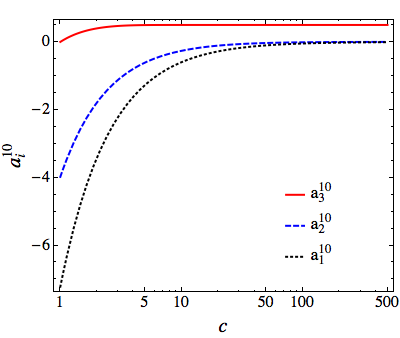
The parameter $c=\pi\Lambda/M_{KK}$ represents the cut-off scale in units of the KK scale and, to consistently describe the first few KK modes within our effective theory, we take $c\geq 10$. To neglect higher-dimensional operators contributing to fermion masses we will show that a value of $c$ larger than 10 is required. To reproduce the large top Yukawa coupling we have to take $a^{10}_{3}=\mu_{3}+k_{X}\approx y_{t}/2$. The hierarchy among the first, second and third generations of quarks can be reproduced by choosing $\mu_{3}\approx y_{t}/2$ and $|k_{X}|,|\mu_{1,2}|\ll 1$. For example, the values of $a^{10}_{i}$ required to generate $(n^{10}_{1},n^{10}_{2},n^{10}_{3})=(\lambda^{4},\lambda^{2},1)$ are shown in Fig. 1, as a function of $c$. For large $c$, $a^{10}_{3}$ approaches to $0.5$ while $|a^{10}_{1,2}|$ go like $1/c$. In terms of our input parameters, we approximately have $\mu_{3}\approx 0.5$, while $|k_{X}|,~{}|\mu_{1,2}|$ are ${\cal O}(1/c)$.

The parameter $c$, describing the gap between the cut-off scale and the KK scale, characterizes the domain of validity of our effective theory. Here we estimate how large $c$ can be in our model and how small can be the ratio $M_{\rm GUT}/\Lambda$, which controls the non-leading contributions to the Yukawa interactions on the $y=0$ brane. A relation between $c$ and the GUT scale parameters such as $k_{X}$ can be derived from the phenomenological requirement $|\mu_{1,2}|\sim|k_{X}|\approx 1/c$, needed to successfully fit the fermion spectrum. There are several scales relevant to the breaking of the grand unified symmetry SO(10): $\upsilon_{\Phi}$, $\langle{\bf 126}_{H}\rangle$, $\langle\overline{\bf 126}_{H}\rangle$, $\langle{\bf 45}_{H}\rangle$. In first approximation we make no distinction among them and we assume $M_{\rm GUT}\approx\upsilon_{\Phi}$. From Eq. (9) and using $|k_{X}|\sim 1/c$, one can express the VEV of the ${\bf 45}_{\Phi}$ in terms of $c$ as:

$$\upsilon_{\Phi}=\left(\frac{1}{2g_{4}^{2}}\right)^{1/3}\frac{\Lambda}{c}~{},$$ (20)

where we use $g_{5}^{2}=\pi Rg_{4}^{2}$. Considering a dimensionless coupling $g_{4}\sim{\cal O}(1)$, one finds

$$\frac{M_{\rm GUT}}{\Lambda}\approx\frac{1}{c}~{},$$ (21)

showing that in the preferred region of parameter space the GUT scale and the KK scale are close to each other. To conveniently suppress the higher order contribution to the Yukawa interactions on the $y=0$ brane we can take $c=100$ and the cut-off $\Lambda$ approximately corresponds to the Planck scale. The bulk mass parameters relevant to our analysis, $m_{i}$ and $\upsilon_{\Phi}$, are all around the GUT scale, except $m_{3}$ which should be relatively close to $\Lambda$.

IV Fermion mass relations and Numerical Analysis

We now derive the effective mass matrices of fermion zero modes in the model and discuss their viability through a detailed numerical analysis. As noted earlier, the light fields ${\bf 10}_{H}$ and ${\bf 120}_{H}$ respectively contain one and two pairs of MSSM-like Higgs doublets. As it is arranged by the missing partner mechanism, one pair of their linear combinations remains massless and plays the role of the MSSM Higgs doublets, namely $H_{u}$ and $H_{d}$. Hence each of the doublets $H_{u,d}^{1}\in{\bf 10}_{H}$ and $H_{u,d}^{2,3}\in{\bf 120}_{H}$ has a component of $H_{u}$ or $H_{d}$ which can conveniently be parametrized in terms of mixing parameters $\alpha_{i}$ and $\bar{\alpha}_{i}$ such that $H_{u}^{i}=\alpha_{i}H_{u}$ and $H_{d}^{i}=\bar{\alpha}_{i}H_{d}$. The appropriate normalizations of $H_{u}$ and $H_{d}$ then require

$$\sum_{i=1}^{3}|\alpha_{i}|^{2}=\sum_{i=1}^{3}|\bar{\alpha}_{i}|^{2}=1.$$ (22)

The VEVs of MSSM Higgs doublets are fixed by the electroweak symmetry breaking scale and are denoted by $\langle H_{u}\rangle=\upsilon\sin\beta$ and $\langle H_{d}\rangle=\upsilon\cos\beta$ with $\upsilon=174$ GeV.

The brane Yukawa couplings of Dirac type fermions are obtained as the linear combinations of only two matrices, $Y_{10}$ and $Y_{120}$, weighted by the appropriate Clebsch-Gordan (CG) coefficients and Higgs mixing parameters $\alpha_{i}$, $\bar{\alpha}_{i}$ Barbieri et al. (1980); Aulakh and Garg (2012):

$$Y_{u} = c_{1}^{u}\alpha_{1}Y_{10}+(c_{2}^{u}\alpha_{2}+c_{3}^{u}\alpha_{3})Y_{120}~{},$$

$$Y_{d} = c_{1}^{d}\bar{\alpha}_{1}Y_{10}+(c_{2}^{d}\bar{\alpha}_{2}+c_{3}^{d}\bar{\alpha}_{3})Y_{120}~{},$$

$$Y_{\nu} = c_{1}^{\nu}\alpha_{1}Y_{10}+(c_{2}^{\nu}\alpha_{2}+c_{3}^{\nu}\alpha_{3})Y_{120}~{},$$

$$Y_{e} = c_{1}^{e}\bar{\alpha}_{1}Y_{10}+(c_{2}^{e}\bar{\alpha}_{2}+c_{3}^{e}\bar{\alpha}_{3})Y_{120}~{},$$ (23)

where $Y_{u,d,e,\nu}$ are Yukawa matrices for up-type quarks, down-type quarks, charged leptons and Dirac neutrinos. The $Y_{10}$ and $Y_{120}$ are symmetric and anti-symmetric matrices respectively in generation space. The CG coefficients can be read as $c_{1}^{u}=c_{1}^{d}=c_{1}^{e}=c_{1}^{\nu}=2\sqrt{2}$, $c_{2}^{u}=c_{2}^{d}=c_{2}^{e}=c_{2}^{\nu}=-2\sqrt{2}$ and $-3c_{3}^{u}=-3c_{3}^{d}=c_{3}^{e}=c_{3}^{\nu}=-2i\sqrt{6}$ Aulakh and Garg (2012). A doublet $H_{d}^{3}$ residing in ${\bf 120}_{H}$ couples to the charged leptons and down-type quarks with different CG coefficients and provides the correction to the wrong mass relation $Y_{d}=Y_{e}$ predicted in the presence of only ${\bf 10}_{H}$. The above $Y_{u}$, $Y_{d}$ and $Y_{e}$ are substituted in Eq. (10) to obtain the effective Yukawa matrices ${\cal Y}_{u}$, ${\cal Y}_{d}$ and ${\cal Y}_{e}$ of the charged fermion zero modes at the GUT scale.

The RH neutrinos get mass from the Yukawa interactions of ${\bf 16}$ with ${\bf\overline{126}}_{H}$ when the SU(5) singlet in ${\bf\overline{126}}_{H}$ acquires a VEV. The mass matrix of the RH neutrino zero modes takes the form

$$M_{R}\equiv\upsilon_{R}~{}F_{1}Y_{126}F_{1}~{}.$$ (24)

Note that $\upsilon_{R}\equiv\langle{\bf\overline{126}}_{H}\rangle$ also contributes in canceling the D-terms and is required to be close to the GUT scale in the absence of any fine tuning. The mass matrix for the light neutrinos generated by the canonical seesaw mechanism can be written as

$$M_{\nu}=-\frac{\upsilon^{2}\sin^{2}\beta}{\upsilon_{R}}~{}F_{\bar{5}}~{}Y_{\nu}Y^{-1}_{126}Y_{\nu}^{T}~{}F_{\bar{5}}\equiv-\frac{\upsilon^{2}\sin^{2}\beta}{\upsilon_{R}}~{}{\cal Y}_{\nu}~{}.$$ (25)

The hierarchy in light neutrino masses is solely governed by the matrix $F_{\bar{5}}$ and, as we will see, it leads to relatively less hierarchical neutrinos in comparison to the charged fermions as arranged by SO(10) breaking in the bulk. Also, the origin of large (but not special values of) lepton mixing angles is apparent in this case. The seesaw mechanism is often seen as the origin of small hierarchies and large mixing in the neutrinos compared to the quark sector. For example, in the mechanism known as seesaw enhancement Smirnov (1993), such a difference can be realized if RH neutrinos have strong hierarchy or they are almost degenerate and Dirac neutrino Yukawas as hierarchical in structure as those of up-type quarks. We would like to emphasize here that hierarchy in the RH neutrino masses in this model is not responsible for enhancement in the leptonic mixing angles as can be seen from Eq. (25). In fact since the RH neutrino unifies with other fermions in SO(10), the hierarchy in their masses can be predicted from the common bulk mass parameters once the appropriate profiles of charged fermions are obtained.

In principle the SU(2)_L triplet contained in ${\bf\overline{126}}_{H}$ can generate an additional contribution to the neutrino masses through the so-called type II seesaw mechanism Lazarides et al. (1981); *Schechter:1980gr; *Mohapatra:1980yp. The coupling of ${\bf\overline{126}}_{H}$ to SO(10) multiplets containing light Higgs doublets induces an effective VEV for such a triplet of order $\upsilon^{2}\sin^{2}\beta/M_{\rm GUT}$. In our model, the missing partner mechanism assumes the absence of a direct coupling among ${\bf\overline{126}}_{H}$ and the two SO(10) multiplets hosting the light Higgs doublets. For example, ${\bf\overline{126}}_{H}$ does not have an SO(10) invariant tree level couplings with two ${\bf 10}_{H}$ or with two ${\bf 120}_{H}$ or with ${\bf 10}_{H}$ and ${\bf 120}_{H}$. Further, any such couplings through higher-dimensional operators are assumed to be absent in the missing partner mechanism. Hence, we do not expect type II seesaw contribution to the light neutrino masses and consider only type I seesaw as the mechanism at work for the light neutrino masses in the following analysis.

IV.1 Fitting the fermion mass spectrum: a viability test

The Yukawa matrices, ${\cal Y}_{u,d,e,\nu}$ which follow from Eqs. (10,IV,25) are predicted at the GUT scale and we compare them with a representative set of data obtained by extrapolating the measured values of fermion masses and mixing parameters. This strategy has been largely followed in the studies based on varieties of SO(10) models in four dimensions, see Bertolini et al. (2006); *Grimus:2006rk; *Altarelli:2010at; *Joshipura:2011nn; *Dueck:2013gca; *Altarelli:2013aqa for examples. It is clear that an extrapolation over more than 14 orders of magnitude is potentially affected by large uncertainties. This is even more true in our model where SUSY breaking effects have been neglected. We are aware that the data we are going to fit at the GUT scale might not faithfully represent the low-energy experimental quantities and that the best fit values of the input parameters we will obtain might considerably change depending on the spectrum of the SUSY particles and the other heavy modes at the GUT scale. We are more interested in the performances of the present model, and we are confident that if it can successfully reproduce a representative set of data, it will also be successful if this set is modified to account for a more realistic framework.

The renormalization group evolution (RGE) of fermion masses in the MSSM primarily depends on the SUSY breaking scale $M_{\rm SUSY}$ and $\tan\beta$. In our numerical study we use, as an idealized set of data at the GUT scale, extrapolated values of the charged fermion masses and the quark mixing parameters from Ross and Serna (2008) which, in a 2-loop analysis, assumes an effective SUSY breaking scale $M_{\rm SUSY}=0.5$ TeV and considers different values of $\tan\beta$. To assess the dependence on $\tan\beta$ we will focus on two cases: $\tan\beta=10$ and $\tan\beta=50$. For the neutrino masses and mixing angles, we use their low-energy values obtained by one of the recent global fits Capozzi et al. (2013); Gonzalez-Garcia et al. (2012); Forero et al. (2014) ignoring the RGE effects from the low scale to the GUT scale. The running of the neutrino masses and mixing angles in the MSSM is known to be negligible in case of $\tan\beta\>\raisebox{-4.73611pt}{$\stackrel{{\scriptstyle\textstyle<}}{{\sim}}$}\>30$. It remains small even for large $\tan\beta$ if the neutrino mass spectrum is hierarchical. As we show later in this section, the model analyzed here favours large $\tan\beta$ and strongly hierarchical spectrum for neutrinos with the lightest neutrino mass $\>\raisebox{-4.73611pt}{$\stackrel{{\scriptstyle\textstyle<}}{{\sim}}$}\>0.005$ eV at the GUT scale. For such a hierarchical neutrino spectrum, the RGE running in the neutrino parameters can be considered negligible to a good approximation Chankowski and Pokorski (2002); Antusch et al. (2003); *Antusch:2005gp. The GUT scale values of different observables we use in our analysis are listed in Table 1. We would like to note that the given extrapolated values do not take into account the threshold corrections in the fermion masses and mixing angles arising from the SUSY breaking. Estimation of such corrections requires precise knowledge of sparticle spectrum which depends on the exact details of SUSY breaking mechanism Hall et al. (1994); *Blazek:1995nv; *Pierce:1996zz which is not studied here. Further, the threshold corrections may also arise at the GUT scale which can be estimated only if the complete mass spectrum of all the GUT multiplets is known. As it is often done in the similar kind of analysis Bertolini et al. (2006); *Grimus:2006rk; *Altarelli:2010at; *Joshipura:2011nn; *Dueck:2013gca; *Altarelli:2013aqa, we ignore these effects and assume that if the model under consideration can fit the idealized GUT scale data listed in Table 1 then it would also be compatible with the real data.

Observables	$\tan\beta=10$	$\tan\beta=50$
$y_{t}$	$0.48\pm 0.02$	$0.51\pm 0.03$
$y_{b}$	$0.051\pm 0.002$	$0.37\pm 0.02$
$y_{\tau}$	$0.070\pm 0.003$	$0.51\pm 0.04$
$m_{u}/m_{c}$	$0.0027\pm 0.0006$	$0.0027\pm 0.0006$
$m_{d}/m_{s}$	$0.051\pm 0.007$	$0.051\pm 0.007$
$m_{e}/m_{\mu}$	$0.0048\pm 0.0002$	$0.0048\pm 0.0002$
$m_{c}/m_{t}$	$0.0025\pm 0.0002$	$0.0023\pm 0.0002$
$m_{s}/m_{b}$	$0.019\pm 0.002$	$0.016\pm 0.002$
$m_{\mu}/m_{\tau}$	$0.059\pm 0.002$	$0.050\pm 0.002$
$|V_{us}|$	$0.227\pm 0.001$
$|V_{cb}|$	$0.037\pm 0.001$
$|V_{ub}|$	$0.0033\pm 0.0006$
$J_{CP}$	$0.000023\pm 0.000004$
$\Delta_{S}/10^{-5}$ eV2	$7.54\pm 0.26$  (NO or IO)
$\Delta_{A}/10^{-3}$ eV2	$2.44\pm 0.08$ (NO)   $2.40\pm 0.07$ (IO)
$\sin^{2}\theta_{12}$	$0.308\pm 0.017$ (NO or IO)
$\sin^{2}\theta_{23}$	$0.425\pm 0.029$ (NO)   $0.437\pm 0.029$ (IO)
$\sin^{2}\theta_{13}$	$0.0234\pm 0.0022$ (NO)   $0.0239\pm 0.0021$ (IO)

Table 1: The GUT scale values of the charged fermion masses and quark mixing parameters from Ross and Serna (2008) that we use in our analysis. The lepton mixing angles and solar and atmospheric mass differences are taken from a global fit analysis Capozzi et al. (2013) ignoring the running effects. NO (IO) stands for the normal (inverted) ordering in the neutrino masses.

We now proceed to the details of fitting procedure. Let us first calculate the total number of free parameters in this model. As already mentioned, $Y_{10}$ and $Y_{126}$ are complex symmetric matrices and $Y_{120}$ is a complex anti-symmetric matrix in generation space. Without loss of generality, we can absorb three phases from $Y_{10}$ into the ${\bf 16}_{i}$ by a suitable redefinition ${\bf 16}_{i}\to e^{i\alpha_{i}}{\bf 16}_{i}$. Hence $Y_{10}$ can be parametrized in terms of 9 real parameters, namely 3 real diagonal elements and 3 complex off-diagonal ones. $Y_{126}$ ($Y_{120}$) contains 12 (6) real parameters. All the Yukawa couplings are regarded as generic order-one quantities in this model and we constrain them within a narrow range, i.e. $0.5\leq|(Y_{10})_{ij}|,~{}|(Y_{126})_{ij}|,~{}|(Y_{120})_{ij}|\leq 1.5$ with arbitrary phases. The parameters $\alpha_{1}$, $\bar{\alpha}_{1}$ in Eq. (IV) can be taken real without loss of generality and can be obtained from $\alpha_{2,3}$, $\bar{\alpha}_{2,3}$ using the normalization condition, Eq. (22). This leaves eight real parameters in $\alpha_{i}$ and $\bar{\alpha}_{i}$ with the constraints $|\alpha_{i}|,~{}|\bar{\alpha}_{i}|<1$, a VEV $\upsilon_{R}$ in Eq. (25) and four real parameters in the profiles of zero-mode fermions as described in Eq. (9). In total, we have 27 ${\cal O}(1)$ real parameters as Yukawa couplings and other 13 real parameters which should correctly reproduce the 18 observables listed in Table 1 if the model is viable.

The values of the free parameters of the model are estimated using the $\chi^{2}$ optimization technique which is widely used in Bertolini et al. (2006); *Grimus:2006rk; *Altarelli:2010at; *Joshipura:2011nn; *Dueck:2013gca; *Altarelli:2013aqa for similar kind of analysis. We define a $\chi^{2}$ function

$$\chi^{2}=\sum_{i}^{n}\left(\frac{P_{i}(x_{1},x_{2},..,x_{m})-O_{i}}{\sigma_{i}}\right)^{2},$$ (26)

where $P_{i}$ are the observable quantities derived from Eqs. (10, IV, 25) as complex nonlinear functions of the free parameters of the model. $O_{i}$ and $\sigma_{i}$ are the GUT scale central values and $1\sigma$ deviations respectively of the corresponding quantities listed in Table 1. The effective Yukawa matrices ${\cal Y}_{u,d,e,\nu}$ are numerically diagonalized and we obtain the diagonal Yukawas as the eigenvalues of ${\cal Y}_{f}$ for each sector. For example, the eigenvalues of ${\cal Y}_{u}$ correspond to $y_{u},~{}y_{c},~{}y_{t}$. The absolute values of the third generation Yukawas and appropriate ratios for the first two generations are included in the $\chi^{2}$ to fit them to their extrapolated experimental values. The quark and lepton mixing parameters are also evaluated in a similar way. For simplicity, we include a ratio $\Delta_{S}/\Delta_{A}$ in $\chi^{2}$ instead of $\Delta_{S}$ and $\Delta_{A}$ individually. As can be seen from Eq. (25), such a ratio and lepton mixing parameters do not depend on $\upsilon_{R}$. The value of $\upsilon_{R}$ can be obtained later from the fit using the absolute scale of atmospheric neutrino oscillation. This allows us to remove one observable and one free parameter from the fit. The $\chi^{2}$ function contains only dimensionless quantities. It is then numerically minimized using the downhill-simplex algorithm incorporated in the software tools MINUIT developed by CERN to determine the best fit values of the parameters $x_{i}$. From the fitted parameters, one can derive the predictions for the various observables which have not been measured yet such as Dirac CP phase in the leptonic sector, the lightest neutrino mass, the effective mass of neutrinoless double beta decay.

As a preliminary step we fit all the $39$ free parameters of the model using $17$ observables mentioned above. Even though many of the free parameters are restricted within narrow ranges of ${\cal O}(1)$ or should face additional constraints like the one of Eq. (22), the number of free parameters are significantly larger than the number of observables. Nevertheless, considering the complex and non-linear dependence of the observable quantities from the input parameters, it is not completely evident that the model can successfully fit the data. We have carried out the $\chi^{2}$ minimization for two different data set corresponding to $\tan\beta=10$ and $50$. Also, each case is analyzed for different ordering of the neutrino masses, i.e. normal (NO) and inverted (IO). The results of fits are reported in Table 2. We obtain very good fit to the data in case of $\tan\beta=50$ and for both the NO and IO in neutrino masses. In particular, the NO case results into a very good fit in which all the observables from the theory fall well into the experimentally allowed range, as can be seen from Table 2. The predictions for various observables obtained at the best fit are also listed in the table. The set of input parameters at the minimum of $\chi^{2}$ are collected in Appendix for both cases. From the best fit in NO case, one obtains a hierarchical profile matrix $F_{10}\approx{\tt diag.}(\lambda^{3.7},\lambda^{2.4},1)$ for 10-plets and a relatively less hierarchical $F_{\bar{5}}\approx{\tt diag.}(\lambda^{1.5},\lambda^{0.9},1)$ for $\bar{5}$-plets as it was expected from the SO(10) breaking effects in the bulk. Such an effect is mostly due to the parameter $k_{X}$ which contributes universally in different flavours. As it can be seen from the best fit values reported in the Appendix, $k_{X}$ is required to be ${\cal O}(\mu_{1,2})$ in order to distinguish between the mass hierarchies among the first and second generations of fermions residing in 10 and ${\bar{5}}$ of SU(5). As a result, the bulk mass parameter of the third generation $\mu_{3}$ dominates over $k_{X}$ and the effective bulk masses $a^{r}_{3}$ are nearly equal for both $r=10$ and $r={\bar{5}}$. Thus an approximate $t-b-\tau$ Yukawa unification at the GUT scale is enforced. As it is well known, the bottom and tau Yukawas unify with that of top quark for large $\tan\beta\geq 45$ Ananthanarayan et al. (1991); *Ananthanarayan:1992cd and hence the model provides a good fit to the data only for $\tan\beta=50$. We obtain very poor fits for $\tan\beta=10$ corresponding to $\chi^{2}_{\rm min}\approx 110$ for NO and $\chi^{2}_{\rm min}\approx 280$ for IO. The large values of the $\chi^{2}_{\rm min}$ in these cases are mainly due to the top, bottom and tau Yukawas, which cannot be fitted simultaneously to their extrapolated values.

	Normal ordering		Inverted ordering
Observable	Fitted value	Pull	Fitted value	Pull
$y_{t}$	0.51	0	0.54	1.00
$y_{b}$	0.37	0	0.37	0
$y_{\tau}$	0.51	0	0.47	-1.00
$m_{u}/m_{c}$	0.0027	0	0.0031	0.67
$m_{d}/m_{s}$	0.051	0	0.045	-0.86
$m_{e}/m_{\mu}$	0.0048	0	0.0048	0
$m_{c}/m_{t}$	0.0023	0	0.0023	0
$m_{s}/m_{b}$	0.016	0	0.015	-0.50
$m_{\mu}/m_{\tau}$	0.050	0	0.049	-0.50
$|V_{us}|$	0.227	0	0.227	0
$|V_{cb}|$	0.037	0	0.038	1.00
$|V_{ub}|$	0.0033	0	0.0030	-0.50
$J_{CP}$	0.000023	0	0.000021	-0.51
$\Delta_{S}/\Delta_{A}$	0.0309	0	0.0320	0.73
$\sin^{2}\theta_{12}$	0.308	0	0.309	0.06
$\sin^{2}\theta_{23}$	0.425	0	0.435	-0.07
$\sin^{2}\theta_{13}$	0.0234	0	0.0237	-0.10
$\chi^{2}_{\rm min}$		$\approx 0$		$\approx 5.75$
	Predicted value		Predicted value
$m_{\nu_{\rm lightest}}$ [meV]	$0.08$		$2.15$
$|m_{\beta\beta}|$ [meV]	1.63		$30.4$
$\sin\delta^{l}_{CP}$	0.265		0.510
$M_{N_{1}}$ [GeV]	$3.85\times 10^{6}$		$1.13\times 10^{4}$
$M_{N_{2}}$ [GeV]	$9.31\times 10^{7}$		$3.06\times 10^{6}$
$M_{N_{3}}$ [GeV]	$2.19\times 10^{14}$		$2.02\times 10^{13}$
$\upsilon_{R}$ [GeV]	$0.05\times 10^{16}$		$0.18\times 10^{16}$

Table 2: Results from numerical fit corresponding to minimized $\chi^{2}$ for normal (NO) and inverted ordering (IO) in neutrino masses. The fit is carried out for the GUT scale extrapolated data given in Table 1 for $\tan\beta=50$. The input parameters are collected in Appendix.

The best fit obtained for IO and $\tan\beta=50$ is also shown in the Table 2. The minimized value of $\chi^{2}$ is relatively large compared to the one obtained for NO but is acceptable as all the observables are fitted within the $1\sigma$ range of their experimental values. Note that the fitted profiles of the light neutrinos, i.e. $F_{\bar{5}}\sim{\tt diag.}(\lambda^{0.8},\lambda^{0.4},1)$, still follows the normal ordering structure (with a slightly less hierarchical structure compared to that of NO case) while ${\cal O}(1)$ Yukawas in $Y_{126}$ conspire to create inverted ordering in the neutrino masses. The mismatch between the hierarchies in neutrinos and charged fermions can be attributed more to a tuning of the ${\cal O}(1)$ Yukawa couplings, rather than to an effect of the zero-mode profiles. We expect that such a solution is very sensitive to the Yukawa parameters in $Y_{126}$ and that even small deviations from their best fit values can significantly raise the $\chi^{2}_{\rm min}$. We investigate this issue in the following subsection.

IV.2 Anarchical Yukawas: a test of naturalness

So far the analysis implies that the model under consideration predicts approximate $t-b-\tau$ Yukawa unification which is compatible only with large values of $\tan\beta$. Moreover both the normal and inverted ordering in the neutrino masses seem to be viable as indicated by the best fit solutions. We do not know yet whether a successful fit in the two cases requires a special tuning of the ${\cal O}(1)$ Yukawa parameters or not. In the present approach this question is relevant, since the whole construction is based on the idea of anarchy in the Yukawa sector: the hierarchical pattern of fermion masses and mixing angles is entirely due to the zero-mode profiles, while the Yukawa couplings on the brane have no structure. If special relations between the ${\cal O}(1)$ Yukawa parameters were needed in order to reproduce the data, this would represent a fine-tuning problem of our model, which cannot appeal to symmetry or dynamical principles to justify such relations. If, on the contrary, the present model were natural, we would expect that a successful explanation of fermion masses and mixing angles should not depend very much on the specific choices of ${\cal O}(1)$ parameters.

To investigate this feature, we have repeated the above analysis with some changes. We randomly varied each of the complex elements in $Y_{10}$, $Y_{126}$ and $Y_{120}$ such that $|Y_{ij}|\in[0.5,1.5]$ and ${\tt arg}(Y_{ij})\in[0,2\pi]$, using flat distributions for both. For a given set of random Yukawa couplings, the $\chi^{2}$ is minimized versus the remaining $12$ parameters (4 bulk masses and 8 Higgs mixing parameters $\alpha_{i}$, $\bar{\alpha}_{i}$) using the $17$ observables described earlier. Unlike the previous case we investigate $10^{5}$ samples of random ${\cal O}(1)$ Yukawas and perform a $\chi^{2}$ minimization for each case. The analysis is carried out for $\tan\beta=50$ and for both NO and IO, as only these cases were found in good agreement with the GUT scale data in the previous analysis, where also the Yukawa couplings were fitted.

The results are displayed in Fig. 2 where we show the distributions of $\chi^{2}_{\rm min}/\nu$, $\nu=5$ being the number of independent degrees of freedom (d.o.f.) in the fit.

Figure 2: The distributions of minimized $\chi^{2}/\nu$ for NO and IO in neutrino masses and for $\tan\beta=50$.

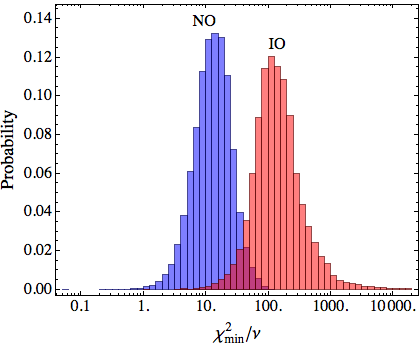
The distribution for NO is clearly peaked at lower values of $\chi^{2}_{\rm min}/\nu$, with respect to the one for IO. In Table 3 we report the number of successful cases for different threshold values of $\chi^{2}_{\rm min}/\nu$ together with the goodness of fit measured in terms of $p-$values.

$p-$value	0.50	0.10	0.05	0.001
$\chi^{2}_{\rm min}/\nu$ (for $\nu=5$)	$\leq$ 0.87	$\leq$ 1.85	$\leq$ 2.21	$\leq$ 4.10
successful cases (NO)	0.1%	0.7%	1.2%	5.6%
successful cases (IO)	$<10^{-3}$%	$<10^{-3}$%	${\bf 10}^{\bf-3}$%	0.01%

Table 3: The fraction of successful events obtained for different $p-$values from random samples of ${\cal O}(1)$ Yukawa couplings in case of normal and inverted ordering in the neutrino masses.

The threshold $p\geq 0.05$ is often considered as an acceptable value for the statistical validity of a fit. As it can be seen from Table 3, in the NO case $p$ is larger than $0.05$ in about one percent of the generated samples, while in the IO case only one over total $10^{5}$ samples reaches the modest $p$-value of $0.05$. Hence the NO turns out as a more natural choice in this model.

In the NO case one percent can be regarded as the size of the required tuning to reproduce the data within the framework of anarchy. It is clear that this number has no absolute meaning and could only be useful if compared with analogous numbers obtained by analyzing other models with a similar approach. A success rate of order $0.01$ is a typical outcome in this kind of analysis for the most successful models Altarelli et al. (2003); Buchmuller et al. (2012); *Bergstrom:2014owa.

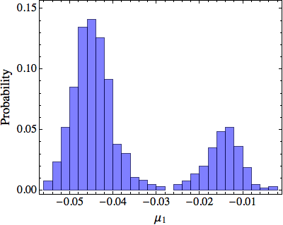
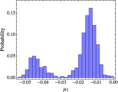
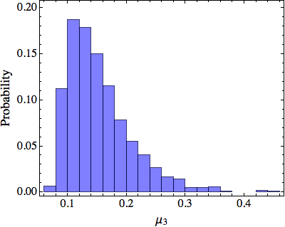
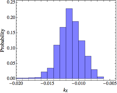
The probability distributions for the bulk mass parameters obtained in 1.2% of the NO cases corresponding to $p\geq 0.05$ are shown in Fig. 3. One finds $\mu_{3}>\mu_{2}\geq\mu_{1}$ in most of the cases as expected and $k_{X}$ turns out to be ${\cal O}(\mu_{1,2})$. A few cases described by smaller peaks in the distributions of $\mu_{1}$ and $\mu_{2}$ corresponds to $\mu_{1}>\mu_{2}$. However, such cases are equivalent to the cases with $\mu_{1}<\mu_{2}$ as one can always interchange ${\bf 16}_{1}\leftrightarrow{\bf 16}_{2}$ by interchanging $\mu_{1}$ and $\mu_{2}$ and also the first and second rows and columns of all the Yukawa coupling matrices on the brane. Such a transformation on Yukawa matrices still preserves their anarchical structure and both these pictures lead to the same physical scenario. As it can be seen from Fig. 3, the preferred values of all the bulk masses remain well below the cut-off scale, and they do not endanger the validity of the effective theory. The $k_{X}<0$ leads to a relatively weak hierarchy among the down-type quarks and charged leptons in comparison to that in the up-type quarks. From the most probable values of $\mu_{i}$ and $k_{X}$ of Fig. 3 we get,

$$F_{10}\simeq\lambda^{0.4}~{}{\tt diag}(\lambda^{4.1},\lambda^{2.2},1)~{}~{}{\rm and}~{}~{}F_{\bar{5}}\simeq\lambda^{0.3}~{}{\tt diag}(\lambda^{1.5},\lambda^{0.7},1).$$ (27)

The above profiles of zero modes provide a quantitative understanding of the differences between the quarks and lepton masses and mixing patterns.

Figure 3: The distributions of bulk mass parameters fitted with $\chi^{2}_{\rm min}/\nu<2.21$ in case of NO and $\tan\beta=50$.

The successful cases corresponding to $\chi^{2}_{\rm min}/\nu<2.21$ can also be used to derive the predictions for the other observables in the lepton sector. The probability distributions for the leptonic Dirac CP phase, the lightest neutrino mass and the effective mass of neutrinoless double beta decay $|m_{\beta\beta}|$ are shown in Fig. 4.

Figure 4: The predictions for various observables obtained for $\chi^{2}_{\rm min}/\nu<2.21$ in case of NO and $\tan\beta=50$.

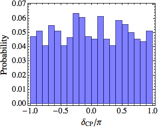
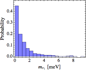
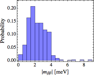
One finds an almost uniform distribution in $\delta^{l}_{CP}$ and the entire range in CP phase is allowed by the model. The lightest neutrino mass is restricted to be $\lesssim 5$ meV corresponding to a hierarchical neutrino mass spectrum while $|m_{\beta\beta}|$ is predicted in the range 0.1-5 meV. Both these predictions are far from the sensitivity of current generation experiments and any positive signal in these experiments would essentially rule out the model.

The predictions for the RH neutrino masses and the VEV of ${\overline{\bf 126}_{H}}$ are displayed in Fig. 5. The bulk masses of the singlets in ${\bf 16}_{i}$ are predicted from the fitted values of $\mu_{i}$ and $k_{X}$. From their most probable values, we obtain

$$F_{1}\simeq\lambda^{0.6}~{}{\tt diag}(\lambda^{7.0},\lambda^{5.0},1)~{}.$$ (28)

This results into an extremely hierarchical mass spectrum for the RH neutrinos corresponding to $M_{N_{1}}\approx\lambda^{15}\upsilon_{R}$, $M_{N_{2}}\approx\lambda^{11}\upsilon_{R}$ and $M_{N_{3}}\approx\lambda\upsilon_{R}$, as shown in the left panel of Fig. 5. As explained earlier, the masses of the RH neutrinos do not play any role in the seesaw mechanism but they can be important for leptogenesis. For a hierarchical mass spectrum of RH neutrinos, a successful thermal leptogenesis requires the mass of the lightest RH neutrino $M_{N_{1}}\gtrsim 10^{9}$ GeV Davidson and Ibarra (2002); *Buchmuller:2002rq in a standard flavour independent scheme. When flavour effects are considered, it is possible to generate a sufficient lepton asymmetry through the decay of the next-to-lightest neutrinos if $10^{12}~{}{\rm GeV}\gtrsim M_{N_{2}}\gtrsim 10^{9}~{}{\rm GeV}$ and $M_{N_{1}}\ll 10^{9}$ GeV as suggested in Di Bari (2005); *Bertuzzo:2010et; *DiBari:2013qja. Both these alternatives cannot be realized in this model, which predicts $M_{N_{1}}\ll M_{N_{2}}<10^{9}$ GeV.

Figure 5: The predictions for the masses of RH neutrinos and the VEV of ${\overline{\bf 126}_{H}}$ obtained for $\chi^{2}_{\rm min}/\nu<2.21$ in case of NO and $\tan\beta=50$.

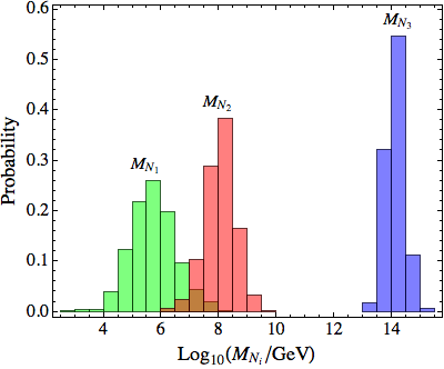
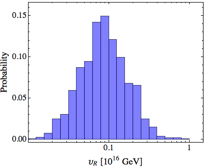
The scale of atmospheric neutrino oscillation requires the VEV of ${\overline{\bf 126}_{H}}$ at least an order of magnitude below $M_{\rm GUT}$, as it can be seen from Fig. 5. This is compatible with the D-term cancellation condition, Eq. (17). As can be seen from Fig. 3, the viable fits to the fermion masses and mixing angles require $\upsilon_{\Phi}^{3/2}=k_{X}\Lambda/(\sqrt{2}g_{5})<0$. Hence the VEV of ${\bf 126}_{H}$ can cancel the D-term in Eq. (17) even if $|\langle{\overline{\bf 126}_{H}}\rangle|\ll|\langle{\bf 126}_{H}\rangle|\sim M_{\rm GUT}$.

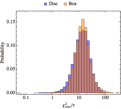
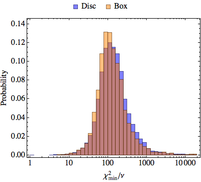
We conclude this section with a comment on the choice of the ${\cal O}(1)$ Yukawa parameters. For the above analysis, we have randomly chosen them from a flat distribution of points residing on the disc of inner radius 0.5 and outer radius 1.5 in a complex plane. To assess the dependence of our results on the criteria for selecting the Yukawa parameters, we have repeated a similar analysis for random Yukawa couplings residing in the box of vertices $(1+i,-1+i,-1-i,1-i)$ in a complex plane. The results are shown in Fig. 6 where we compare the probability distributions obtained for the two choices of Yukawa parameters. The obtained distributions are almost indistinguishable and the new choice leads to nearly the same results as the old one. The overall results and predictions derived in this subsection are therefore robust and should stand for similar choices of ${\cal O}(1)$ parameters.

Figure 6: A comparison between the minimized $\chi^{2}$ distributions obtained from the two different distribution of random ${\cal O}(1)$ Yukawa couplings (see text for the details). The left (right) panel corresponds to the NO (IO) case and $\tan\beta=50$.

V Conclusions

Anarchical Yukawa matrices for both quarks and leptons can be nicely reconciled with the observed fermion masses and mixing angles by appealing to wave-function renormalizations that distinguish generations and fermion species. This naturally occurs in models with an extra spatial dimension, thanks to the different localization of the profiles of fermion zero modes. Such a picture is also compatible with SU(5) grand unification, at least in first approximation. The large mixing angles of the lepton sector and the moderate hierarchy among neutrino masses is attributed to a nearly equal wave function renormalization of the three generations of $\bar{5}$. The observed hierarchies in the charged lepton sector and in the quark sectors are mostly due to the different renormalization affecting the three generations of $10$. The different rescaling of $\bar{5}$-plets and 10-plets implies that mass ratios in the up-quark sector are nearly the square of the corresponding mass ratios in the down-quark and charged-lepton sectors, which is approximately true. Such a description can be extended to SO(10), as shown in a five-dimensional model by Kitano and Li. Before SO(10) breaking, all members of a fermion generation, hosted in a ${\bf 16}$ representation, have the same zero-mode profile, which depends upon an SO(10) invariant bulk mass term. In the Kitano-Li model SO(10) is broken down to the direct product of SU(5) and U(1)_X, by the VEV of an SO(10) adjoint that lives in the bulk and has gauge coupling to matter supermultiplets. In this way different bulk mass terms for the SU(5) multiplets residing in the same ${\bf 16}$ representation are generated, with corresponding different zero-mode profiles.

In this paper we have reconsidered the Kitano-Li model. To start with, we have modified it in such a way that fermion masses and mixing angles are dominated by Yukawa interaction terms of the same dimensionality, while in the original model non-renormalizable operators of different mass dimensions had to provide comparable contributions to achieve a realistic description. We have also included a set of Higgs multiplets that allows for a solution to the doublet-triplet splitting problem through the missing partner mechanism. We have explicitly specified the set of interactions needed in order to implement such a mechanism. Finally, we have tested the validity of the model by realizing a series of fits to an idealized set of 17 data, obtained by naively extrapolating fermion masses and mixing angles from low energy to the GUT scale. Our model depends on 27 anarchical Yukawa couplings, 8 parameters characterizing the light Higgs combinations and 4 parameters that describe the fermion bulk masses. In a first fit we left all parameters to vary freely and we obtained an excellent agreement with data for both the cases of normal and inverted ordered neutrino spectrum, for large values of $\tan\beta$. Despite the large number of free parameters, we consider such an agreement not completely trivial, given the fact that 35 of our parameters can vary in a very limited interval close to one and that only the 4 parameters describing the bulk masses are responsible for all the observed hierarchies in the fermion spectrum. In a second stage, to detect a possible fine-tuning among the anarchical Yukawa couplings, we have modified our numerical analysis by first generating a random sample of ${\cal O}(1)$ Yukawa couplings and by subsequently fitting the remaining 12 Higgs and bulk parameters. This procedure have been iterated to obtain a distribution of minimum $\chi^{2}$ values. We see a clear difference between the cases of normal ordering and inverted ordering in the neutrino masses. While in the inverted ordering case we need about $10^{5}$ samples to reach a $p$-value close to $0.05$, in the normal hierarchy case in about one percent of the cases we have $p>0.05$. This unambiguously indicates that our model needs a severe fine-tuning of the “anarchical” parameters in the case of inverted ordered neutrino spectrum while the normally ordered one is accommodated much more naturally.

We verified that these results are stable versus changes in the drawing of the anarchical parameters. Our analysis is incomplete under several respects. In particular we have not discussed the breaking of $N=1$ supersymmetry. This would have allowed to reduce the uncertainty in the extrapolation of fermion masses and mixing angles from low-energy to the GUT scale, at the cost of a much bigger model dependence. Consequently we were not able to analyze the rich related phenomenology of flavour and CP violations, both in the quark and in the lepton sector, which heavily depends on the chosen mechanism for supersymmetry breaking.

Concerning predictions, we have found no preference for any particular value of the leptonic Dirac CP phase. The lightest neutrino mass should lie below $5$ meV, corresponding to a hierarchical neutrino mass spectrum while $|m_{\beta\beta}|$ is predicted in the range 0.1-5 meV. Any positive signal in the current generation of experiments aiming at measuring neutrino masses or $|m_{\beta\beta}|$ in the lab would essentially rule out the model. The hierarchy in the right handed neutrino spectrum is very pronounced and the corresponding mass distributions are peaked around $10^{6}$ GeV, $10^{8}$ GeV and $10^{14}$ GeV. As a consequence, thermal leptogenesis cannot be responsible for the observed baryon asymmetry in our model. On a more qualitative side, our analysis confirms that the idea of anarchical Yukawa couplings can be successfully implemented even in the context of an SO(10) grand unified theory. The required conditions are that SO(10) is broken down to SU(5) as a first step and that the anarchical Yukawa couplings of the different charge sectors are not entirely dominated by a single SO(10) Higgs multiplet. Special features of neutrino data, such as the indications of a nearly maximal atmospheric mixing angle and hierarchical light neutrino spectrum should be regarded as fully accidental in this approach, devoid of any implications on the underlying dynamics.

Appendix A Parameters obtained for the best fit solutions

We give here the input parameters obtained for the best fit solutions presented in the Table 2 corresponding to normal and inverted neutrino mass spectrum and $\tan\beta=50$.

A.1 Normal ordering

The best fit values of the Yukawa matrices and various parameters appearing in Eqs. (IV, 25) at $\chi^{2}_{\rm min}\approx 0$ are listed below.

$$Y_{10} = \left(\begin{array}[]{ccc}0.78314&1.05610e^{1.79809i}&0.92306e^{-0.19874i}\\ 1.05610e^{1.79809i}&1.49012&1.09077e^{1.02405i}\\ 0.92306e^{-0.19874i}&1.09077e^{1.02405i}&0.96156\end{array}\right)~{},$$ (32)

$$Y_{120} = \left(\begin{array}[]{ccc}0&1.04750e^{-2.22311i}&0.50164e^{3.02587i}\\ -1.04750e^{-2.22311i}&0&0.78048e^{-0.43312i}\\ -0.50164e^{3.02587i}&-0.78048e^{-0.43312i}&0\end{array}\right)~{},$$ (36)

$$Y_{126} = \left(\begin{array}[]{ccc}1.49976e^{1.45362i}&0.51701e^{-1.20768i}&1.25349e^{-1.82494i}\\ 0.51701e^{-1.20768i}&0.50067e^{-0.49914i}&0.91593e^{0.05375i}\\ 1.25349e^{-1.82494i}&0.91593e^{0.05375i}&1.38243e^{-1.37536i}\end{array}\right)~{}.$$ (40)

$$\alpha_{2} = 0.87373~{}e^{-2.05269i}~{},~{}~{}\alpha_{3}=0.06975~{}e^{-1.21499i}~{},$$

$$\overline{\alpha}_{2} = 0.81115~{}e^{-1.00683i}~{},~{}~{}\overline{\alpha}_{3}=0.50212~{}e^{-1.20195i}~{}.$$ (41)

The bulk mass parameters are:

$$\{\mu_{1},~{}\mu_{2},~{}\mu_{3},~{}k_{X}\} = \{-0.03732,~{}-0.01565,~{}0.20467,~{}-0.01031\}~{}.$$ (42)

From the above parameters and using Eq. (11), one obtains the following zero-mode profiles of various SU(5) multiplets at $y=0$.

$$F_{10}=\lambda^{0.3}\left(\begin{array}[]{ccc}\lambda^{3.7}&0&0\\ 0&\lambda^{2.4}&0\\ 0&0&1\end{array}\right),~{}F_{\bar{5}}=\lambda^{0.3}\left(\begin{array}[]{ccc}\lambda^{1.5}&0&0\\ 0&\lambda^{0.9}&0\\ 0&0&1\end{array}\right),~{}F_{1}=\lambda^{0.4}\left(\begin{array}[]{ccc}\lambda^{6.2}&0&0\\ 0&\lambda^{4.8}&0\\ 0&0&1\end{array}\right).$$ (52)

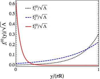
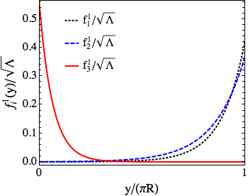
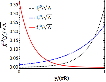
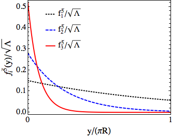
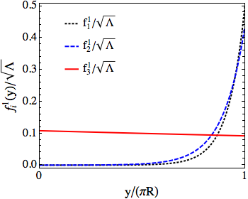
Further, the localization of zero-mode profiles of different generations of 10, ${\bar{5}}$ and 1 can be obtained by replacing $m\rightarrow m_{i}^{r}$ in Eq. (2) and are displayed in Fig. 7.

Figure 7: The localized zero-mode profiles of different SU(5) matter multiplets for the best fit solution obtained in case of normal ordering in the neutrino masses.

A.2 Inverted ordering

The best fit values of the Yukawa matrices and various parameters appearing in Eqs. (IV, 25) at $\chi^{2}_{\rm min}\approx 5.75$ are listed below.

$$Y_{10} = \left(\begin{array}[]{ccc}0.50232&1.12746e^{-0.07927i}&1.25370e^{-0.46501i}\\ 1.12746e^{-0.07927i}&0.74605&1.49999e^{0.94538i}\\ 1.25370e^{-0.46501i}&1.49999e^{0.94538i}&1.38633\end{array}\right)~{},$$ (56)

$$Y_{120} = \left(\begin{array}[]{ccc}0&0.53486e^{2.05559i}&1.29570e^{2.53388i}\\ -0.53486e^{2.05559i}&0&0.58945e^{-0.03658i}\\ -1.29570e^{2.53388i}&-0.58945e^{-0.03658i}&0\end{array}\right)~{},$$ (60)

$$Y_{126} = \left(\begin{array}[]{ccc}1.49999e^{0.16531i}&0.50005e^{1.43459i}&0.58661e^{-2.24612i}\\ 0.50005e^{1.43459i}&0.50007e^{-0.86236i}&1.02973e^{-1.58869i}\\ 0.58661e^{-2.24612i}&1.02973e^{-1.58869i}&0.96577e^{-0.16857i}\end{array}\right)~{}.$$ (64)

$$\alpha_{2} = 0.04681~{}e^{1.46923i}~{},~{}~{}\alpha_{3}=0.07100~{}e^{3.10679i}~{},$$

$$\overline{\alpha}_{2} = 0.87191~{}e^{0.46323i}~{},~{}~{}\overline{\alpha}_{3}=0.36100~{}e^{-1.36707i}~{}.$$ (65)

The bulk mass parameters are:

$$\{\mu_{1},~{}\mu_{2},~{}\mu_{3},~{}k_{X}\} = \{-0.040351,~{}-0.01099,~{}0.085029,~{}-0.01668\}~{}.$$ (66)

From the above parameters and using Eq. (11), one obtains the following zero-mode profiles of various SU(5) multiplets at $y=0$.

$$F_{10}=\lambda^{0.7}\left(\begin{array}[]{ccc}\lambda^{3.9}&0&0\\ 0&\lambda^{2.2}&0\\ 0&0&1\end{array}\right),~{}F_{\bar{5}}=\lambda^{0.4}\left(\begin{array}[]{ccc}\lambda^{0.8}&0&0\\ 0&\lambda^{0.4}&0\\ 0&0&1\end{array}\right),~{}F_{1}=\lambda^{1.5}\left(\begin{array}[]{ccc}\lambda^{7.4}&0&0\\ 0&\lambda^{5.5}&0\\ 0&0&1\end{array}\right).$$ (76)

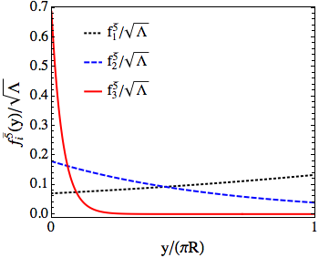
Further, the localization of zero-mode profiles of different generations of 10, ${\bar{5}}$ and 1 fermions can be obtained by replacing $m\rightarrow m_{i}^{r}$ in Eq. (2) and are displayed in Fig. 8.

Figure 8: The localized zero-mode profiles of different SU(5) matter multiplets for the best fit solution obtained in case of inverted ordering in the neutrino masses.

References

- Georgi and Glashow (1974) H. Georgi and S. Glashow, Phys.Rev.Lett. 32, 438 (1974).
- Fritzsch and Minkowski (1975) H. Fritzsch and P. Minkowski, Annals Phys. 93, 193 (1975).
- Minkowski (1977) P. Minkowski, Phys.Lett. B67, 421 (1977).
- Yanagida (1979) T. Yanagida, Conf.Proc. C7902131, 95 (1979).
- Gell-Mann et al. (1979) M. Gell-Mann, P. Ramond, and R. Slansky, Conf.Proc. C790927, 315 (1979), arXiv:1306.4669 [hep-th] .
- Glashow (1980) S. Glashow, NATO Adv.Study Inst.Ser.B Phys. 59, 687 (1980).
- Lazarides et al. (1981) G. Lazarides, Q. Shafi, and C. Wetterich, Nucl.Phys. B181, 287 (1981).
- Schechter and Valle (1980) J. Schechter and J. Valle, Phys.Rev. D22, 2227 (1980).
- Mohapatra and Senjanovic (1981) R. N. Mohapatra and G. Senjanovic, Phys.Rev. D23, 165 (1981).
- Fukugita and Yanagida (1986) M. Fukugita and T. Yanagida, Phys.Lett. B174, 45 (1986).
- Giunti et al. (1991) C. Giunti, C. Kim, and U. Lee, Mod.Phys.Lett. A6, 1745 (1991).
- Amaldi et al. (1991) U. Amaldi, W. de Boer, and H. Furstenau, Phys.Lett. B260, 447 (1991).
- Langacker and Luo (1991) P. Langacker and M.-x. Luo, Phys.Rev. D44, 817 (1991).
- Babu and Mohapatra (1993) K. Babu and R. Mohapatra, Phys.Rev.Lett. 70, 2845 (1993), arXiv:hep-ph/9209215 [hep-ph] .
- Oda et al. (1999) K.-y. Oda, E. Takasugi, M. Tanaka, and M. Yoshimura, Phys.Rev. D59, 055001 (1999), arXiv:hep-ph/9808241 [hep-ph] .
- Bertolini et al. (2004) S. Bertolini, M. Frigerio, and M. Malinsky, Phys.Rev. D70, 095002 (2004), arXiv:hep-ph/0406117 [hep-ph] .
- Babu and Macesanu (2005) K. Babu and C. Macesanu, Phys.Rev. D72, 115003 (2005), arXiv:hep-ph/0505200 [hep-ph] .
- Bertolini and Malinsky (2005) S. Bertolini and M. Malinsky, Phys.Rev. D72, 055021 (2005), arXiv:hep-ph/0504241 [hep-ph] .
- Bertolini et al. (2006) S. Bertolini, T. Schwetz, and M. Malinsky, Phys.Rev. D73, 115012 (2006), arXiv:hep-ph/0605006 [hep-ph] .
- Grimus and Kuhbock (2007) W. Grimus and H. Kuhbock, Eur.Phys.J. C51, 721 (2007), arXiv:hep-ph/0612132 [hep-ph] .
- Altarelli and Blankenburg (2011) G. Altarelli and G. Blankenburg, JHEP 1103, 133 (2011), arXiv:1012.2697 [hep-ph] .
- Joshipura and Patel (2011) A. S. Joshipura and K. M. Patel, Phys.Rev. D83, 095002 (2011), arXiv:1102.5148 [hep-ph] .
- Dueck and Rodejohann (2013) A. Dueck and W. Rodejohann, JHEP 1309, 024 (2013), arXiv:1306.4468 [hep-ph] .
- Altarelli and Meloni (2013) G. Altarelli and D. Meloni, JHEP 1308, 021 (2013), arXiv:1305.1001 .
- Aulakh and Garg (2012) C. S. Aulakh and S. K. Garg, Nucl.Phys. B857, 101 (2012), arXiv:0807.0917 [hep-ph] .
- Aulakh (2011) C. S. Aulakh, (2011), arXiv:1107.2963 [hep-ph] .
- Clark et al. (1982) T. Clark, T.-K. Kuo, and N. Nakagawa, Phys.Lett. B115, 26 (1982).
- Aulakh and Mohapatra (1983) C. Aulakh and R. N. Mohapatra, Phys.Rev. D28, 217 (1983).
- Aulakh et al. (2004) C. S. Aulakh, B. Bajc, A. Melfo, G. Senjanovic, and F. Vissani, Phys.Lett. B588, 196 (2004), arXiv:hep-ph/0306242 [hep-ph] .
- Bajc et al. (2008) B. Bajc, I. Dorsner, and M. Nemevsek, JHEP 0811, 007 (2008), arXiv:0809.1069 [hep-ph] .
- Melfo et al. (2010) A. Melfo, A. Ramirez, and G. Senjanovic, Phys.Rev. D82, 075014 (2010), arXiv:1005.0834 [hep-ph] .
- Grimus and Kuhbock (2006) W. Grimus and H. Kuhbock, Phys.Lett. B643, 182 (2006), arXiv:hep-ph/0607197 [hep-ph] .
- Grimus and Kuhbock (2008) W. Grimus and H. Kuhbock, Phys.Rev. D77, 055008 (2008), arXiv:0710.1585 [hep-ph] .
- Joshipura et al. (2009) A. S. Joshipura, B. P. Kodrani, and K. M. Patel, Phys.Rev. D79, 115017 (2009), arXiv:0903.2161 [hep-ph] .
- Matsuda et al. (2001) K. Matsuda, Y. Koide, and T. Fukuyama, Phys.Rev. D64, 053015 (2001), arXiv:hep-ph/0010026 [hep-ph] .
- Matsuda et al. (2002) K. Matsuda, Y. Koide, T. Fukuyama, and H. Nishiura, Phys.Rev. D65, 033008 (2002), arXiv:hep-ph/0108202 [hep-ph] .
- Fukuyama and Okada (2002) T. Fukuyama and N. Okada, JHEP 0211, 011 (2002), arXiv:hep-ph/0205066 [hep-ph] .
- Fukuyama et al. (2005) T. Fukuyama, A. Ilakovac, T. Kikuchi, S. Meljanac, and N. Okada, Eur.Phys.J. C42, 191 (2005), arXiv:hep-ph/0401213 [hep-ph] .
- Albright et al. (1998) C. H. Albright, K. Babu, and S. M. Barr, Phys.Rev.Lett. 81, 1167 (1998), arXiv:hep-ph/9802314 [hep-ph] .
- Babu et al. (2000) K. Babu, J. C. Pati, and F. Wilczek, Nucl.Phys. B566, 33 (2000), arXiv:hep-ph/9812538 [hep-ph] .
- Dermisek and Raby (2005) R. Dermisek and S. Raby, Phys.Lett. B622, 327 (2005), arXiv:hep-ph/0507045 [hep-ph] .
- Dermisek et al. (2006) R. Dermisek, M. Harada, and S. Raby, Phys.Rev. D74, 035011 (2006), arXiv:hep-ph/0606055 [hep-ph] .
- Barbieri et al. (1997) R. Barbieri, L. J. Hall, S. Raby, and A. Romanino, Nucl.Phys. B493, 3 (1997), arXiv:hep-ph/9610449 [hep-ph] .
- Albright and Barr (2000) C. H. Albright and S. M. Barr, Phys.Rev. D62, 093008 (2000), arXiv:hep-ph/0003251 [hep-ph] .
- Albright and Barr (2001) C. H. Albright and S. M. Barr, Phys.Rev. D64, 073010 (2001), arXiv:hep-ph/0104294 [hep-ph] .
- Ji et al. (2006) X.-d. Ji, Y.-c. Li, and R. Mohapatra, Phys.Lett. B633, 755 (2006), arXiv:hep-ph/0510353 [hep-ph] .
- Alciati et al. (2006) M. L. Alciati, F. Feruglio, Y. Lin, and A. Varagnolo, JHEP 0611, 039 (2006), arXiv:hep-ph/0603086 [hep-ph] .
- Hagedorn et al. (2009) C. Hagedorn, M. A. Schmidt, and A. Y. Smirnov, Phys.Rev. D79, 036002 (2009), arXiv:0811.2955 [hep-ph] .
- King and Malinsky (2006) S. F. King and M. Malinsky, JHEP 0611, 071 (2006), arXiv:hep-ph/0608021 [hep-ph] .
- King and Luhn (2009) S. F. King and C. Luhn, Nucl.Phys. B820, 269 (2009), arXiv:0905.1686 [hep-ph] .
- King and Luhn (2010) S. F. King and C. Luhn, Nucl.Phys. B832, 414 (2010), arXiv:0912.1344 [hep-ph] .
- Dutta et al. (2010) B. Dutta, Y. Mimura, and R. Mohapatra, JHEP 1005, 034 (2010), arXiv:0911.2242 [hep-ph] .
- Patel (2011) K. M. Patel, Phys.Lett. B695, 225 (2011), arXiv:1008.5061 [hep-ph] .
- Bhupal Dev et al. (2011) P. Bhupal Dev, R. Mohapatra, and M. Severson, Phys.Rev. D84, 053005 (2011), arXiv:1107.2378 [hep-ph] .
- Bhupal Dev et al. (2012) P. Bhupal Dev, B. Dutta, R. Mohapatra, and M. Severson, Phys.Rev. D86, 035002 (2012), arXiv:1202.4012 [hep-ph] .
- Chen and Mahanthappa (2003) M.-C. Chen and K. Mahanthappa, Int.J.Mod.Phys. A18, 5819 (2003), arXiv:hep-ph/0305088 [hep-ph] .
- Fukuyama (2013) T. Fukuyama, Int.J.Mod.Phys. A28, 1330008 (2013), arXiv:1212.3407 [hep-ph] .
- Kitano and Li (2003) R. Kitano and T.-j. Li, Phys.Rev. D67, 116004 (2003), arXiv:hep-ph/0302073 [hep-ph] .
- Froggatt and Nielsen (1979) C. Froggatt and H. B. Nielsen, Nucl.Phys. B147, 277 (1979).
- Kaplan (1991) D. B. Kaplan, Nucl.Phys. B365, 259 (1991).
- Csaki et al. (2008) C. Csaki, A. Falkowski, and A. Weiler, JHEP 0809, 008 (2008), arXiv:0804.1954 [hep-ph] .
- Masiero et al. (1982) A. Masiero, D. V. Nanopoulos, K. Tamvakis, and T. Yanagida, Phys.Lett. B115, 380 (1982).
- Grinstein (1982) B. Grinstein, Nucl.Phys. B206, 387 (1982).
- Babu et al. (2007) K. Babu, I. Gogoladze, and Z. Tavartkiladze, Phys.Lett. B650, 49 (2007), arXiv:hep-ph/0612315 [hep-ph] .
- Babu et al. (2012) K. Babu, I. Gogoladze, P. Nath, and R. M. Syed, Phys.Rev. D85, 075002 (2012), arXiv:1112.5387 [hep-ph] .
- Altarelli et al. (2003) G. Altarelli, F. Feruglio, and I. Masina, JHEP 0301, 035 (2003), arXiv:hep-ph/0210342 [hep-ph] .
- Altarelli et al. (2012) G. Altarelli, F. Feruglio, I. Masina, and L. Merlo, JHEP 1211, 139 (2012), arXiv:1207.0587 [hep-ph] .
- Sato and Yanagida (1998) J. Sato and T. Yanagida, Phys.Lett. B430, 127 (1998), arXiv:hep-ph/9710516 [hep-ph] .
- Buchmuller and Yanagida (1999) W. Buchmuller and T. Yanagida, Phys.Lett. B445, 399 (1999), arXiv:hep-ph/9810308 [hep-ph] .
- Pomarol and Quiros (1998) A. Pomarol and M. Quiros, Phys.Lett. B438, 255 (1998), arXiv:hep-ph/9806263 [hep-ph] .
- Arkani-Hamed et al. (2002) N. Arkani-Hamed, T. Gregoire, and J. G. Wacker, JHEP 0203, 055 (2002), arXiv:hep-th/0101233 [hep-th] .
- Barbieri et al. (2002) R. Barbieri, R. Contino, P. Creminelli, R. Rattazzi, and C. Scrucca, Phys.Rev. D66, 024025 (2002), arXiv:hep-th/0203039 [hep-th] .
- Arkani-Hamed and Schmaltz (2000) N. Arkani-Hamed and M. Schmaltz, Phys.Rev. D61, 033005 (2000), arXiv:hep-ph/9903417 [hep-ph] .
- Mirabelli and Schmaltz (2000) E. A. Mirabelli and M. Schmaltz, Phys.Rev. D61, 113011 (2000), arXiv:hep-ph/9912265 [hep-ph] .
- Kaplan and Tait (2001) D. E. Kaplan and T. M. Tait, JHEP 0111, 051 (2001), arXiv:hep-ph/0110126 [hep-ph] .
- Dimopoulos and Wilczek (1981) S. Dimopoulos and F. Wilczek, Print-81-0600 (SANTA BARBARA), NSF-ITP-82-07 (1981).
- Barr and Raby (1997) S. M. Barr and S. Raby, Phys.Rev.Lett. 79, 4748 (1997), arXiv:hep-ph/9705366 [hep-ph] .
- Babu and Barr (1993) K. Babu and S. M. Barr, Phys.Rev. D48, 5354 (1993), arXiv:hep-ph/9306242 [hep-ph] .
- Ross and Serna (2008) G. Ross and M. Serna, Phys.Lett. B664, 97 (2008), arXiv:0704.1248 [hep-ph] .
- Barbieri et al. (1980) R. Barbieri, D. V. Nanopoulos, G. Morchio, and F. Strocchi, Phys.Lett. B90, 91 (1980).
- Lavoura et al. (2006) L. Lavoura, H. Kuhbock, and W. Grimus, Nucl.Phys. B754, 1 (2006), arXiv:hep-ph/0603259 [hep-ph] .
- Smirnov (1993) A. Y. Smirnov, Phys.Rev. D48, 3264 (1993), arXiv:hep-ph/9304205 [hep-ph] .
- Capozzi et al. (2013) F. Capozzi, G. Fogli, E. Lisi, A. Marrone, D. Montanino, et al., (2013), arXiv:1312.2878 [hep-ph] .
- Gonzalez-Garcia et al. (2012) M. Gonzalez-Garcia, M. Maltoni, J. Salvado, and T. Schwetz, JHEP 1212, 123 (2012), arXiv:1209.3023 [hep-ph] .
- Forero et al. (2014) D. Forero, M. Tortola, and J. Valle, (2014), arXiv:1405.7540 [hep-ph] .
- Chankowski and Pokorski (2002) P. H. Chankowski and S. Pokorski, Int.J.Mod.Phys. A17, 575 (2002), arXiv:hep-ph/0110249 [hep-ph] .
- Antusch et al. (2003) S. Antusch, J. Kersten, M. Lindner, and M. Ratz, Nucl.Phys. B674, 401 (2003), arXiv:hep-ph/0305273 [hep-ph] .
- Antusch et al. (2005) S. Antusch, J. Kersten, M. Lindner, M. Ratz, and M. A. Schmidt, JHEP 0503, 024 (2005), arXiv:hep-ph/0501272 [hep-ph] .
- Hall et al. (1994) L. J. Hall, R. Rattazzi, and U. Sarid, Phys.Rev. D50, 7048 (1994), arXiv:hep-ph/9306309 [hep-ph] .
- Blazek et al. (1995) T. Blazek, S. Raby, and S. Pokorski, Phys.Rev. D52, 4151 (1995), arXiv:hep-ph/9504364 [hep-ph] .
- Pierce et al. (1997) D. M. Pierce, J. A. Bagger, K. T. Matchev, and R.-j. Zhang, Nucl.Phys. B491, 3 (1997), arXiv:hep-ph/9606211 [hep-ph] .
- Ananthanarayan et al. (1991) B. Ananthanarayan, G. Lazarides, and Q. Shafi, Phys.Rev. D44, 1613 (1991).
- Ananthanarayan et al. (1993) B. Ananthanarayan, G. Lazarides, and Q. Shafi, Phys.Lett. B300, 245 (1993).
- Buchmuller et al. (2012) W. Buchmuller, V. Domcke, and K. Schmitz, JHEP 1203, 008 (2012), arXiv:1111.3872 [hep-ph] .
- Bergstrom et al. (2014) J. Bergstrom, D. Meloni, and L. Merlo, (2014), arXiv:1403.4528 [hep-ph] .
- Davidson and Ibarra (2002) S. Davidson and A. Ibarra, Phys.Lett. B535, 25 (2002), arXiv:hep-ph/0202239 [hep-ph] .
- Buchmuller et al. (2002) W. Buchmuller, P. Di Bari, and M. Plumacher, Nucl.Phys. B643, 367 (2002), arXiv:hep-ph/0205349 [hep-ph] .
- Di Bari (2005) P. Di Bari, Nucl.Phys. B727, 318 (2005), arXiv:hep-ph/0502082 [hep-ph] .
- Bertuzzo et al. (2011) E. Bertuzzo, P. Di Bari, and L. Marzola, Nucl.Phys. B849, 521 (2011), arXiv:1007.1641 [hep-ph] .
- Di Bari and Marzola (2013) P. Di Bari and L. Marzola, Nucl.Phys. B877, 719 (2013), arXiv:1308.1107 [hep-ph] .