Asymptotically Optimal Sampling-based Kinodynamic Planning

Abstract

Sampling-based algorithms are viewed as practical solutions for high-dimensional motion planning. Recent progress has taken advantage of random geometric graph theory to show how asymptotic optimality can also be achieved with these methods. Achieving this desirable property for systems with dynamics requires solving a two-point boundary value problem (BVP) in the state space of the underlying dynamical system. It is difficult, however, if not impractical, to generate a BVP solver for a variety of important dynamical models of robots or physically simulated ones. Thus, an open challenge was whether it was even possible to achieve optimality guarantees when planning for systems without access to a BVP solver. This work resolves the above question and describes how to achieve asymptotic optimality for kinodynamic planning using incremental sampling-based planners by introducing a new rigorous framework. Two new methods, STABLE_SPARSE_RRT (SST) and SST^∗, result from this analysis, which are asymptotically near-optimal and optimal, respectively. The techniques are shown to converge fast to high-quality paths, while they maintain only a sparse set of samples, which makes them computationally efficient. The good performance of the planners is confirmed by experimental results using dynamical systems benchmarks, as well as physically simulated robots.

1 Introduction

Kinodynamic Planning: For many interesting robots it is difficult to adapt a collision-free path into a feasible one given the underlying dynamics. This class of robots includes ground vehicles at high-velocities (Likhachev & Ferguson (2009)), unmanned aerial vehicles, such as fixed-wing airplanes (Richter et al. (2013)), or articulated robots with dynamics, including balancing and locomotion systems (Kuindersma et al. (2014)). In principle, most robots controlled by the second-order derivative of their configuration (e.g., acceleration, torque) and which exhibit drift cannot be treated by a decoupled approach for trajectory planning given their controllability properties (Laumond et al. (1998); Choset et al. (2005)). To solve such challenges, the idea of kinodynamic planning has been proposed (Donald et al. (1993)), which involves directly searching for a collision-free and feasible trajectory in the underlying system’s state space. This is a harder problem than kinematic path planning, as it involves searching a higher-dimensional space and respecting the underlying flow that arises from the dynamics. Given its importance, however, it has attracted a lot of attention in the robotics community. The focus in this work is on the properties of the popular sampling-based motion planners for kinodynamic challenges (Kavraki et al. (1996); LaValle & Kuffner (2001a); Hsu et al. (2002); Karaman & Frazzoli (2011)).

Sampling-based Motion Planning: The sampling-based approach has been shown to be a practical solution for quickly finding feasible paths for relatively high-dimensional motion planning challenges (Kavraki et al. (1996); LaValle & Kuffner (2001a); Hsu et al. (2002)). The first popular methodology, the Probabilistic Roadmap Method (PRM) (Kavraki et al. (1996)) focused on preprocessing the configuration space of a kinematic system so as to generate a roadmap that can be used to quickly answer multiple queries. Tree-based variants, such as RRT-Extend (LaValle & Kuffner (2001a)) and EST (Hsu et al. (2002)), focused on addressing kinodynamic problems. For all these methods, the guarantee provided is relaxed to probabilistic completeness, i.e., the probability of finding a solution if one exists, converges to one (Kavraki et al. (1998); Hsu et al. (1998); Ladd & Kavraki (2004)). This was seen as a sufficient objective in the community given the hardness of motion planning and the curse of dimensionality. More recently, however, the focus has shifted from providing feasible solutions to achieving high-quality solutions. A milestone has been the identification of the conditions under which sampling-based algorithms are asymptotically optimal. These conditions relate to the connectivity of the underlying roadmap based on results on random geometric graphs (Karaman & Frazzoli (2011)). This line of work provided asymptotically optimal algorithms for motion planning, such as PRM^∗ and RRT^∗ (Karaman & Frazzoli (2010)).

Lack of a BVP Solution: A requirement for the generation of a motion planning roadmap is the existence of a steering function. This function returns the optimum path between two states in the absence of obstacles. In the case of a dynamical system, the steering function corresponds to the solution of a two-point boundary value problem (BVP). Addressing this problem corresponds to solving a differential equation, while also satisfying certain boundary conditions. It is not easy, however, to produce a BVP solution for many interesting dynamical systems and this is the reason that roadmap planners, including the asymptotically optimal PRM^∗, cannot by used for kinodynamic planning.

Unfortunately, RRT^∗ also requires a steering function, as it reasons over an underlying roadmap even though it generates a tree data structure. While in certain cases it is sufficient to plan for a linearized version of the dynamics (Webb & van Den Berg (2013)) or using a numerical approximation to the BVP problem, this approach is not a general solution. Furthermore, it does not easily address an important class of planning challenges, where the system is simulated using a physics engine. In this situation, the primitive available to the planning process is forward propagation of the dynamics using the physics engine. Thus, an open problem for the motion planning community was whether it was even possible to achieve optimality given access only to a forward propagation model of the dynamics.

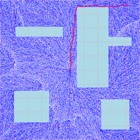
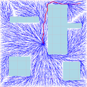
Figure 1: Trees constructed by RRT^∗ (left) and SST (right) for a 2D kinematic point system after 1 minute of computation. Solution paths are shown in red. SST does not require a steering function as RRT^∗ does, making SST more useful in kinodynamic problems.

Summary of Contribution: This paper introduces a new way to analyze the properties of incremental sampling-based algorithms that construct a tree data structure for a wide class of kinodynamic planning challenges. This analysis provides the conditions under which asymptotic optimality can be achieved when a planner has access only to a forward propagation model of the system’s dynamics. The reasoning is based on a kinodynamic system’s accessibility properties and probability theory to argue probabilistic completeness and asymptotic optimality for non-holonomic systems where Chow’s condition holds (Chow, 1940/1941), eliminating the requirement for a BVP solution. Based on these results, a series of sampling-based planners for kinodynamic planning are considered:

1. A simplification of EST, which extends a tree data structure in a random way, referred to as NAIVE_RANDOM_TREE: It is shown to be asymptotically optimal but impractical as it does not have good convergence to high quality paths.

2. An approach inspired by an existing variation of RRT, referred to as RRT-BestNear (Urmson & Simmons (2003)), which promotes the propagation of reachable states with good path cost: It is shown to be asymptotically near-optimal and has a practical convergence rate to high quality paths but has a per iteration cost that is higher than that of RRT.

3. The proposed algorithms STABLE_SPARSE_RRT (SST) and STABLE_SPARSE-RRT^∗ (SST^∗), which use the BestNear selection process. They apply a pruning operation to keep the number of nodes stored small: they are able to achieve asymptotic near-optimality and optimality respectively. They also have good convergence rate to high quality paths. SST has reduced per iteration cost relative to the suboptimal RRT given the pruning operation, which accelerates searching for nearest neighbors.

An illustration of the proposed SST’s performance for a kinematic point system is provided in Fig. 1. This is a simple challenge, where comparison with RRT^∗ is possible. This is a problem where RRT typically does not return a path in the homotopic class of the optimum one. SST is able to do so, while also maintaining a sparse data structure. Fig. 2 describes the performance of different components of SST in searching the phase space of a pendulum system relative to RRT. No method is making use of a steering function for the pendulum system. A summary of the desirable properties of SST and SST^∗ in relation to the efficient RRT and the asymptotically optimal RRT^∗ is available in Table 1.

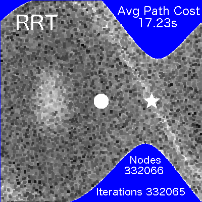
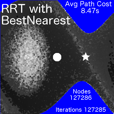
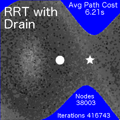
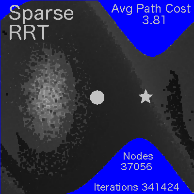
Figure 2: Phase plots that show best path cost at each point in the one-link pendulum state space for each of the proposed modifications (the BestNear primitive and the pruning (mentioned as Drain in the third Figure above)). $x$-axis: pendulum angle, $y$-axis: velocity. Blue corresponds to unexplored regions of the state space. The circle is state $\{0,0\}$, a horizontal placement of the pendulum, the star is state $\{\frac{\pi}{2},0\}$, an upward configuration. Colors are computed by dividing the best path cost to a state in a pixel by a predefined value (20.0 for RRT and 10.0 for the other methods) and then mapping the result to the range [0,255]. All algorithms were executed for the same amount of time (5 min). For the last two methods that provide a sparse representation, each state is coloring a 3x3 local neighborhood. The best path cost for each pixel is displayed.

RRT-Extend	RRT∗	SST/SST∗
Probabilistically Complete (under conditions)	Probabilistically Complete	Probabilistically $\delta$-Robust Complete / Probabilistically Complete
Provably Suboptimal	Asymptotically Optimal	Asymptotically $\delta$-Robust Near-Optimal / Asymptotically Optimal
Forward Propagation	Steering Function	Forward Propagation
Single Propagation Per Iteration	Many Steering Calls Per Iteration	Single Propagation Per Iteration
1 NN Query ($\mathcal{O}(\log N)$)	1 NN + 1 K-Query ($\mathcal{O}(\log N)$)	Bounded Time Complexity Per Iteration / 1 Range Query + 1 NN Query
Includes All Collision-Free Samples	Includes All Collision-Free Samples	Sparse Data Structure / Converges to All Collision-Free Samples

Table 1: Comparing RRT, RRT^∗with the proposed SST / SST^∗, which minimize computation cost and space requirements while providing asymptotic (near-)optimality for kinodynamic planning. This table compares the following from top to bottom: completeness properties, optimality properties, the process for the extension primitive, the number of extensions per iteration, the type of nearest neighbor queries (nearest, k-closest, and range), as well as space complexity. The notion of $\delta$-robustness is introduced in this paper.

Paper Overview: The following section provides a more comprehensive review of the literature and the relative contribution of this paper. Then, Section 3 identifies formally the considered problem and a set of assumptions under which the desired properties for the proposed algorithms hold. Section 4 first outlines how sampling-based algorithms need to be adapted so as to achieve asymptotic optimality and efficiency in the context of kinodynamic planning. Based on this outline, the description of SST and SST^∗ is then provided, as well as an accompanying nearest neighbor data structure, which allows the removal of nodes to achieve a sparse tree. The description of the algorithms is followed by the comprehensive analysis of the described methods in Section 5. Simulation results on a series of systems, including kinematic ones, where comparison with RRT^∗ is possible, as well as benchmarks with interesting dynamics are available in Section 6. A physically simulated system is also considered in the same section. Finally, the paper concludes with a discussion in Section 7.

2 Background

Planning Trajectories: Trajectory planning for real robots requires accounting for dynamics (e.g., friction, gravity, limits in forces). It can be achieved either by a decoupled approach (Bobrow et al., 1985; Shiller & Dubowsky, 1991) or direct planning. The latter method searches the state space of a dynamical system directly. For underactuated, non-holonomic systems, especially those that are not small-time locally controllable (STLC), the direct planning approach is preferred. The focus here is on systems that are not STLC but are small-time locally accessible (Chow, 1940/1941). The following methodologies have been considered in the related literature for direct planning:

• Optimal control can be applied (Brockett, 1982; Lewis & Syrmos, 1995) but handles only simple systems. Algebraic solutions are available primarily for 2D point mass systems (O’Dunlaing, 1987; Canny et al., 1991).

• Numerical optimization (Fernandes et al., 1993; Betts, 1998; Ostrowski et al., 2000) can be used but it can be expensive for global trajectories and suffers from local minima. There has been progress along this direction (Zucker et al., 2013; Schulman et al., 2014), although highly-dynamic problems are still challenging.

• Approaches that take advantage of differential flatness allow to plan for dynamical systems as if they are high-dimensional kinematic ones (Fliess et al., 1995). While interesting robots, such as quadrotors (Sreenath et al., 2013), can be treated in this manner, other systems, such as fixed-wing airplanes, are not amenable to this approach.

• Search-based methods compute paths over discretizations of the state space but depend exponentially on the resolution (Sahar & Hollerbach, 1985; Shiller & Dubowsky, 1988; Barraquand & Latombe, 1993). They also correspond to an active area of research, including for systems with dynamics (Likhachev & Ferguson, 2009).

A polynomial-time, search-based approximation framework introduced the notion of ‘‘kinodynamic’’ planning and solved it for a dynamic point mass (Donald et al., 1993), which was then extended to more complicated systems (Heinzinger et al., 1989; Donald & Xavier, 1995). This work influenced sampling-based algorithms for kinodynamic planning.

Sampling-based Planners: These algorithms avoid explicitly representing configuration space obstacles, which is computationally hard. They instead sample vertices and connect them with local paths in the collision-free state space resulting in a graph data structure. The first popular sampling-based algorithm, the Probabilistic Roadmap Method (PRM) (Kavraki et al., 1996), precomputes a roadmap using random sampling, which is then used to answer multiple queries. RRT-Connect returns a tree and focuses on quickly answering individual queries (Kuffner & Lavalle, 2000). Bidirectional tree variants achieve improved performance (Sanchez & Latombe, 2001). All these solutions require a steering function, which connects two states with a local path ignoring obstacles. For systems with symmetries it is possible to connect bidirectional trees by using numerical methods for bridging the gap between two states (Cheng et al., 2004; Lamiraux et al., 2004).

Two sampling-based methods that do not require a steering function are RRT-Extend (LaValle & Kuffner, 2001a) and Expansive Space Trees (EST) (Hsu et al., 2002). They only propagate dynamics forward in time and aim to evenly and quickly explore the state space regardless of obstacle placement. For all of the above methods, probabilistic completeness can be argued under certain conditions (Kavraki et al. (1998); Hsu et al. (1998); Ladd & Kavraki (2004)). Variants of these approaches aim to decrease the metric dependence by reducing the rate of failed node expansions (Cheng & LaValle, 2001), or applying adaptive state-space subdivision (Ladd & Kavraki, 2005b). Others guide the tree using heuristics (Bekris & Kavraki, 2008), local reachability information (Shkolnik et al., 2009), linearizing locally the dynamics to compute a metric (Glassman & Tedrake, 2010), learning the cost-to-go to balance or bias exploration (Li & Bekris, 2010, 2011), or by taking advantage of grid-based discretizations (Plaku et al., 2010; Şucan & Kavraki, 2012). Such tree-based methods have been applied to various interesting domains (Frazzoli et al., 2002; Branicky et al., 2006; Zucker et al., 2007). While RRT is effective in returning a solution quickly, it converges to a sub-optimal solution (Nechushtan et al., 2010).

From Probabilistic Completeness to Asymptotic Optimality: Some RRT variants have employed heuristics to improve path quality but are not provably optimal (Urmson & Simmons, 2003), including anytime variants (Ferguson & Stentz, 2006). Important progress was achieved through the utilization of random graph theory to rigorously show that roadmap-based approaches, such as PRM^∗ and RRT^∗, can achieve asymptotic optimality (Karaman & Frazzoli, 2011). The requirement is that each new sample must be tested for connection with at least a logarithmic number of neighbors as a function of the total number of nodes using a steering function. Anytime (Karaman et al., 2011) and lazy (Alterovitz et al., 2011) variants of RRT^∗ have also been proposed. There are also techniques that provide asymptotic near-optimality using sparse roadmaps, which inspire the current work (Marble & Bekris, 2011, 2013; Dobson et al., 2012; Dobson & Bekris, 2014; Wang et al., 2013; Shaharabani et al., 2013). Sparse trees appear in the context of feedback-based motion planning (Tedrake, 2009). Another line of work follows a Lazy PRM^∗ approach to improve performance (Janson & Pavone, 2013). A conservative estimate of the reachable region of a system can be constructed (Karaman & Frazzoli, 2013). This reachable region helps to define appropriate metrics under dynamics, and can be used in conjunction with the algorithms described here. All of the above methods, which are focused on returning high-quality paths, require a BVP solver.

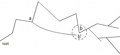
Figure 3: If $b^{\prime}$ is close to $b$ and $cost(b^{\prime})<cost(b)$, the shooting variant will prune the edge to $b$ and replace it with $b^{\prime}$. The subset of $b$ is repropagated from $b^{\prime}$.

Towards Asymptotic Optimality for Dynamical Systems: A variation of RRT^∗ utilizes a ‘‘shooting’’ approach, shown in Figure 3, to improve solutions without a steering function (Jeon et al., 2011). When propagating from node $a$ to state $b^{\prime}$ within a small distance of node $b$ and the cost to $b^{\prime}$ is smaller, $b$ is pruned and an edge from $a$ to $b^{\prime}$ is added. The subtree of $b$ is repropagated from $b^{\prime}$, which may result in node pruning if collisions occur. This method does not provably achieve asymptotic optimality. It can be integrated with numerical methods for decreasing the gap between $b$ and $b^{\prime}$. The methods presented here achieve formal guarantees. Improved computational performance relative to the ‘‘shooting’’ variant is shown in the experimental results. Recent work provides local planners for systems with linear or linearizable dynamics (Webb & van Den Berg, 2013; Goretkin et al., 2013). There are also recent efforts on avoiding the use of an exact steering function (Jeon et al., 2013). The algorithms in the current paper are applicable beyond systems with linear dynamics but could also be combined with the above methods to provide efficient asymptotically near-optimal solvers for such systems.

Closely Related Contributions: Early versions of the work presented here have appeared before. Initially, a simpler version of the proposed algorithms was proposed, called Sparse-RRT (Littlefield et al., 2013). Good experimental performance was achieved with this method, but it was not possible to formally argue desirable properties. This motivated the development of STABLE_SPARSE_RRT (SST) and SST^∗  in follow-up work (Li et al., 2014). These methods formally achieve asymptotic (near)-optimality for kinodynamic planning. The same paper was the first to introduce the analysis that is extended in the current manuscript. Given these earlier efforts by the authors, this paper provides the following contributions:

• It describes a general framework for asymptotic (near-)optimality using sampling-based planners without a steering function in Section 4.1. The SST and SST^∗ algorithms correspond to efficient implementations of this framework.

• It describes for the first time in Section 4.4 a nearest neighbor data structure that has been specifically designed to support the pruning operation of the proposed algorithms. Implementation guidelines are introduced in the description of SST and SST^∗ that improve performance (Sections 4.2 and 9).

• Section 5 extends the analysis by arguing properties for a general cost function instead of trajectory duration. It also provides all the necessary proofs that were missing from previous work.

• Additional experiments are provided in Section 6, including simulations for a dynamical model of a fixed-wing airplane. There is also evaluation of the effects the nearest neighbor data structure has on the motion planners.

There is also concurrent work (Papadopoulos et al., 2014), which presents similar algorithms and argues experimentally that they return high-quality trajectories for kinodynamic planning. It provides a different way to support the argument that a simplification of EST, i.e., the NAIVE_RANDOM_TREE approach, is asymptotically optimal. It doesn’t argue, however, the asymptotic near-optimality properties of the efficient and practical methods that achieve a sparse representation, neither studies the convergence rate of the corresponding algorithms nor provides efficient tools for their implementation, such as the nearest neighbor data structure described here.

3 Problem Setup

This paper considers dynamic systems that respect time-invariant differential equations of the following form:

$$\dot{x}(t)=f(x(t),u(t)),\ \ x(t)\in\mathbb{X},\ \ u(t)\in\mathbb{U}\vspace{-0.05in}$$ (1)

where $x(t)\in\mathbb{X}\subseteq R^{d}$ and $u(t)\in\mathbb{U}\subseteq R^{l}$. The collision-free subset of $\mathbb{X}$ is $\mathbb{X}_{f}$. Let $\mu(\mathbb{X})$ denote the Lebesgue measure of $\mathbb{X}$. This work focuses on state space manifolds that are subsets of $d$-dimensional Euclidean spaces, which allow the definition of the $\mathbb{L}_{2}$ Euclidean norm $||.||$. The corresponding $r$-radius closed ball in $\mathbb{X}$ centered at $x$ will be $\mathcal{B}_{r}(x)$. In other words, the underlying state space needs to exhibit some smoothness properties and behave locally as a Euclidean space.

Definition 1.

(Trajectory) A trajectory $\pi$ is a function $\pi(t):[0,t_{\pi}]\rightarrow\mathbb{X}_{f}$, where $t_{\pi}$ is its duration. A trajectory $\pi$ is generated by starting at a given state $\pi(0)$ and applying a control function $\Upsilon:[0,t_{\pi}]\rightarrow\mathbb{U}$ by forward integrating Eq. 1.

Typically, sampling-based planners are implemented so that the applied control function $\Upsilon$ corresponds to a piecewise constant one. Such an underlying discretization is often unavoidable given the presence of a digital controller. This is why the analysis provided in this paper considers piecewise constant control functions, which are otherwise arbitrary in nature.

Definition 2.

(Piecewise Constant Control Function) A piecewise constant control function $\bar{\Upsilon}$ with resolution $\Delta t$ is the concatenation of constant control functions of the form $\Upsilon_{i}:[0,k_{i}\cdot\Delta t]\rightarrow u_{i}$, where $u_{i}\in\mathbb{U}$ and $k_{i}\in\mathbb{Z}^{+}$.

The proposed methods and the accompanying analysis do not critically depend on the piecewise constant nature of the input control function. They could potentially be extended to also allow for continuous control functions, such as those generated by splines or using basis functions:

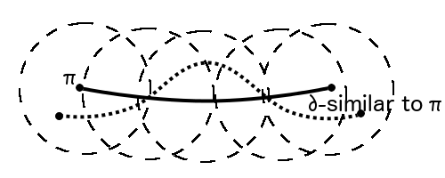
Figure 4: Two $\delta$-similar trajectories.

A key notion for this work is illustrated in Figure 4 and explained below:

Definition 3.

($\delta$-Similar Trajectories) Trajectories $\pi$, $\pi^{\prime}$ are $\delta$-similar if for a continuous, nondecreasing scaling function $\sigma:[0,t_{\pi}]\rightarrow[0,t_{\pi^{\prime}}]$, it is true that $\pi^{\prime}(\sigma(t))\in\mathcal{B}_{\delta}(\pi(t))$.

The focus in this paper will be initially on optimal trajectories with a certain clearance from obstacles.

Definition 4.

(Obstacle Clearance) The obstacle clearance $\epsilon$ of a trajectory $\pi$ is the minimum distance from obstacles over all states in $\pi$, i.e., $\epsilon=\inf_{t\in[0,t_{\pi}],x_{o}\in\mathbb{X}_{o}}\ ||\pi(t)-x_{o}||$, where $\mathbb{X}_{o}=\mathbb{X}\setminus\mathbb{X}_{f}$.

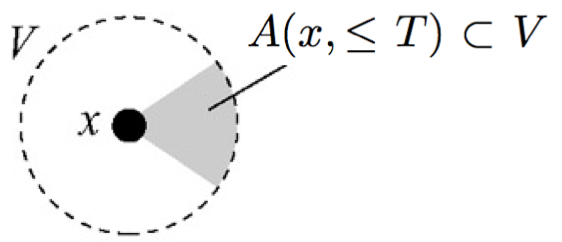
Figure 5: The STLA property.

Then, the following assumption is helpful for the methods and the analysis.

Assumption 5.

The system described by Equation 1 satisfies the properties:

• Chow’s condition (Chow, 1940/1941) of Small-time Locally Accessible (STLA) systems (Choset et al., 2005): For STLA systems, it is true that the reachable set of states $A(x,\leq T)\subset V$ from any state $x$ in time less than or equal to $T$ without exiting a neighborhood $V\subset\mathbb{X}$ of $x$, and for any such $V$, has the same dimensionality as $\mathbb{X}$.

• It has bounded second derivative: $|\ddot{x}(t)|\leq M_{2}\in R^{+}$.

• It is Lipschitz continuous for both of its arguments, i.e., $\exists\ K_{u}>0$ and $\exists\ K_{x}>0$:

  $$||f(x_{0},u_{0})-f(x_{0},u_{1})||\leq K_{u}||u_{0}-u_{1}||,\ \ \ \ \ \ \ \ \ \ \ ||f(x_{0},u_{0})-f(x_{1},u_{0})||\leq K_{x}||x_{0}-x_{1}||.$$

The assumption that $f$ satisfies Chow’s condition implies there always exist $\delta$-similar trajectories for any trajectory $\pi$.

Lemma 6.

Let there be a trajectory $\pi$ for a system satisfying Eq. 1 and Chow’s condition. Then there exists a positive value $\delta_{0}$ called the dynamic clearance, such that: $\forall\ \delta\in(0,\delta_{0}]$, $\forall\ x_{0}^{\prime}\in\mathcal{B}_{\delta}(\pi(0))$, and $\forall\ x_{1}^{\prime}\in\mathcal{B}_{\delta}(\pi(t_{\pi}))$, there exists a trajectory $\pi^{\prime}$, so that: (i) $\pi^{\prime}(0)=x_{0}^{\prime}$ and $\pi^{\prime}(t_{\pi^{\prime}})=x_{1}^{\prime}$; (ii) $\pi$ and $\pi^{\prime}$ are $\delta$-similar trajectories.

Lemma 6 on the existence of ‘‘dynamic clearance’’ is a necessary condition for all systems where sampling-based methods work, such as EST, RRT, and RRT^∗, are able to find a solution. A proof sketch of Lemma 6 can be found in Appendix A. The interest is on trajectories with both good obstacle and dynamic clearance, called $\delta$-robust trajectories.

Definition 7.

($\delta$-Robust Trajectories) A trajectory $\pi$ for a dynamical system following Eq. 1 is called $\delta$-robust if both its obstacle clearance $\epsilon$ and its dynamic clearance $\delta_{0}$ are greater than $\delta$.

This paper aims to solve a variation of the motion planning problem with dynamics for such optimal trajectories.

Definition 8.

($\delta$-Robust Feasible Motion Planning) Given a dynamical system following Eq. 1, the collision-free subset $\mathbb{X}_{f}\subset\mathbb{X}$, an initial state $x_{0}\in\mathbb{X}_{f}$, a goal region $\mathbb{X}_{G}\subset\mathbb{X}_{f}$, and that a $\delta$-robust trajectory that connects $x_{0}$ with a state in $\mathbb{X}_{G}$ exists, find a solution trajectory $\pi$ for which $\pi(0)=x_{0}$ and $\pi(t_{\pi})\in\mathbb{X}_{G}$.

It will be necessary to assume that the problem can be solved using trajectories generated by piecewise constant control functions. This is a reasonable way to generate a trajectory using a computational approach.

Assumption 9.

For a $\delta$-robust feasible motion planning problem, there exists a $\delta$-robust trajectory $\pi$ generated by a piecewise constant control function $\bar{\Upsilon}$.

An incremental sampling-based algorithm, abbreviated here as $ALG$, typically extends a graph data structure of feasible trajectories over multiple iterations. This paper considers the following properties of such sampling-based planners.

Definition 10.

(Probabilistic $\delta$-Robust Completeness) Let $\Pi^{ALG}_{n}$ denote the set of trajectories discovered by an algorithm $ALG$ at iteration $n$. Algorithm $ALG$ is probabilistically $\delta$-robustly complete, if for any $\delta$-robustly feasible motion planning problem ($\mathbb{X}_{f}$, $x_{0}$, $\mathbb{X}_{G}$, $\delta$) the following holds:

$$\liminf_{n\to\infty}\mathbb{P}(\ \exists\ \pi\in\Pi^{ALG}_{n}:\pi\textrm{ solution to }(\mathbb{X}_{f},x_{0},\mathbb{X}_{G},\delta))=1.$$

Definition 10 relaxes the concept of probabilistic completeness for algorithms with properties that depend on the robust clearance $\delta$ of trajectories they can discover. An algorithm that is probabilistically $\delta$-robustly complete only demands it will eventually find solution trajectories if one with robust clearance of $\delta$ exists. The following discussion relates to the cost function of a trajectory $\pi$.

Assumption 11.

The cost function $cost(\pi)$ of a trajectory is assumed to be Lipschitz continuous. Specifically, $\exists\ K_{c}>0$:

$$|{\tt cost}(\pi_{0})-{\tt cost}(\pi_{1})|\leq K_{c}\cdot sup_{\forall t}\{||\pi_{0}(t)-\pi_{1}(t)||\},\vspace{-0.05in}$$

for all $\pi_{1}$, $\pi_{2}$ with the same start state. Consider two trajectories $\pi_{1},\pi_{2}$ such that their concatenation is $\pi_{1}|\pi_{2}$ (i.e., following trajectory $\pi_{2}$ after trajectory $\pi_{1}$), the cost function satisfies:

• $cost(\pi_{1}|\pi_{2})=cost(\pi_{1})+cost(\pi_{2})$ (additivity)

• $cost(\pi_{1})\leq cost(\pi_{1}|\pi_{2})$ (monotonicity)

• $\forall\ t_{2}>t_{1}\geq 0$, $\exists M_{c}>0$, $t_{2}-t_{1}\leq M_{c}\cdot|cost(\pi(t_{2}))-cost(\pi(t_{1}))|$ (non-degeneracy)

Then, it is possible to relax the property of asymptotic optimality and allow some tolerance depending on the clearance.

Definition 12.

(Asymptotic $\delta$-robust Near-Optimality) Let $c^{*}$ denote the minimum cost over all solution trajectories for a $\delta$-robust feasible motion planning problem ($\mathbb{X}_{f}$, $x_{0}$, $\mathbb{X}_{G}$, $\delta$). Let $Y^{ALG}_{n}$ denote a random variable that represents the minimum cost value among all trajectories returned by algorithm $ALG$ at iteration $n$ for the same problem. $ALG$ is asymptotically $\delta$-robust near-optimal if for all independent runs:

$$\mathbb{P}(\Big{\{}\limsup_{n\to\infty}Y_{n}^{ALG}\leq h(c^{\ast},\delta)\Big{\}})=1\vspace{-0.05in}$$

where $h:\mathbb{R}\times\mathbb{R}\rightarrow\mathbb{R}$ is a function of the optimum cost and the $\delta$ clearance, where $h(c^{\ast},\delta)\geq c^{\ast}$.

The analysis will show that the proposed algorithms exhibit the above property where $h$ has the form: $h(c^{\ast},\delta)=(1+\alpha\cdot\delta)\cdot c^{\ast}$ for some constant $\alpha\geq 0$. In this case, $ALG$ is asymptotically $\delta$-robust near-optimal with a multiplicative error. Note that for this form of the $h$ function, the absolute error relative to the optimum cost increases as the optimum cost increases. This property guarantees that the cost of the returned solution is upper bounded relative to the optimal cost. Recall that RRT-Connect returns solutions of random cost and the error is unbounded (Karaman & Frazzoli, 2011).

If it is possible to argue that an algorithm satisfies the last two properties for all decreasing values of the robust clearance $\delta$, then this algorithm satisfies the traditional properties of probabilistic completeness and asymptotic optimality.

Regarding Distances: The true cost of moving between two states corresponds to the ‘‘cost-to-go’’, which typically does not satisfy symmetry, is not the Euclidean distance, and is not easy to compute. Based on the ‘‘cost-to-go’’, it is possible to define an $\epsilon$-radius sub-riemannian ball centered at $x$, which is the set of all states where the ‘‘cost-to-go’’ from $x$ to that set is less than or equal to $\epsilon$. The analysis presented, which reasons primarily over Euclidean hyper-balls, will show that there always exists a certain size Euclidean hyper-ball inside the sub-riemannian ball under the above conditions. Therefore, it will be sufficient to reason about Euclidean norms. In practice, distances may be taken with respect to a different space, which reflect the application, and may actually be closer to the true ‘‘cost-to-go’’ for the moving system.

4 Algorithms

This section provides sampling-based tree motion planners that achieve the properties of Definitions 10 and 12 for kinodynamic planning when there is no access to a BVP solver. First a general framework is described for this purpose, and then an instantiation of this framework is given (SST), which is extended to an asymptotically optimal algorithm (SST^∗).

4.1 Change in Algorithmic Paradigm

Traditional Approach: Given the difficulty of kinodynamic planning (Donald et al. (1993)), the early but practical tree-based planners (LaValle & Kuffner, 2001b; Hsu et al., 2002) aimed for even and fast exploration of $\mathbb{X}$ even in challenging high-dimensional cases where greedy, heuristic expansion towards the goal would fail. Given that computing optimal trajectories corresponds to an even harder challenge, the focus was not on the quality of the returned trajectory in these early methods.

1 $G=\{\mathbb{V}\leftarrow\{x_{0}\},\mathbb{E}\leftarrow\emptyset\}$;

2 for $N$ iterations do

3       $x_{selected}\leftarrow$ Exploration_First_Selection($\mathbb{V},\mathbb{X}$);

4       $x_{new}\leftarrow$ Fixed_Duration_Prop($x_{selected}$, $\mathbb{U}$, $T_{prop}$);

5       if  CollisionFree$(\overline{x_{selected}\to x_{new}})$ then

6             $\mathbb{V}\leftarrow\mathbb{V}\cup\{x_{new}\}$;

7             $\mathbb{E}\leftarrow\mathbb{E}\cup\{\overline{x_{selected}\to x_{new}}\}$;

8            

9      

10return $G(\mathbb{V},\mathbb{E})$;

Algorithm 1 EXPLORATION_TREE($\mathbb{X}$, $\mathbb{U}$, $x_{0}$, $T_{prop}$, $N$)

Algorithm 1 summarizes the high-level selection/propagation operation of these planners. They constructed a graph data structure $G(V,E)$ in the form of a tree rooted at an initial state $x_{0}$ in the following two-step process:

• Selection: A reachable state along the tree, such as a node $x_{selected}\in V$, is selected. In some variants a state along an edge of the tree can also be selected (Ladd & Kavraki, 2005a). The selection process is designed so as to increase the probability of searching underexplored parts of $\mathbb{X}$. For instance, the RRT-Extend algorithm samples a random state $x_{rand}$ and then selects the closest node on the tree as $x_{selected}$. The objective is to achieve a ‘‘Voronoi-bias’’ that promotes exploration, i.e., nodes on the tree that correspond to the largest Voronoi regions of $\mathbb{X}$, given tree nodes as sites, have a higher probability of being selected . In EST implementations, nodes store the local density of samples and those with low density are selected with higher probability to promote exploration (Phillips et al., 2004).

• Propagation: The procedure for extending the tree has varied in the related literature but the scheme followed in RRT-Extend has been popular in most implementations. The approach is to select a control that drives the system towards the randomly sampled point, then forward propagate that control input for a fixed time duration. If the resulting trajectory $\overline{x_{selected}\to x_{new}}$ is collision-free, then it is added as an edge in the tree. It was recently shown that this propagation scheme actually makes RRT-Extend lose its probabilistic completeness guarantees (Kunz & Stilman, 2014). In EST, a randomized approach is employed where random controls are used. The analysis of the proposed methods shows that a randomized approach has benefits in terms of solution quality.

Challenge: Optimality has only recently become the focus of sampling-based motion planning, given the development of the asymptotically optimal RRT^∗ and PRM^∗ (Karaman & Frazzoli, 2011). This great progress, however, does not address kinodynamic planning instances. Both planners are roadmap-based methods in the sense that they reason over (in the case of RRT^∗) or explicitly construct (in the case of PRM^∗) a graph that makes use of a steering function to connect states. This raised the following research challenge in the community:

Is it even possible to achieve asymptotic optimality guarantees in sampling-based kinodynamic planning?

This has been an open question in the algorithmic robotics community and resulted in many methods that aim to provide asymptotic optimality for systems with dynamics (Karaman & Frazzoli, 2013; Webb & van Den Berg, 2013; Goretkin et al., 2013; Jeon et al., 2013). The majority of these techniques, however, can address only specific classes of problems (e.g., systems with linear dynamics) and do not possess the generality of the original sampling-based tree planners.

Progress: The current work provides an answer to the above open question through a comprehensive, novel analysis of sampling-based processes for motion planning without access to a steering function, which departs from previous analysis efforts in this domain. In particular, the following are shown:

1. It is possible to achieve asymptotic optimality in the rather general setting of this paper’s problem setup with a sampling-based process that makes proper use of random forward propagation and a naïve selection strategy.

2. This method, however, is computationally impractical and does not have a good convergence rate to optimal solutions. Thus, the important question is whether there are planners with practical convergence to high-quality solutions.

3. Given this realization, this work describes a framework for computationally efficient sampling-based planners that achieve asymptotic near-optimality, which are then also extended to provide asymptotic optimality.

Asymptotic Optimality from Random Primitives: To achieve these desirable properties it is necessary to clearly define the framework which sampling-based algorithms should adopt. In particular, it is possible to argue asymptotic optimality for the NAIVE_RANDOM_TREE process described in Algorithm 2. This algorithm follows the same selection/propagation scheme of sampling-based tree planners but applies uniform selection and calls the MonteCarlo-Prop procedure to extend the tree.

1 $G=\{\mathbb{V}\leftarrow\{x_{0}\},\mathbb{E}\leftarrow\emptyset\}$;

2 for $N$ iterations do

3       $x_{selected}\leftarrow$ Uniform_Sampling($\mathbb{V}$);

4       $x_{new}\leftarrow$MonteCarlo-Prop( $x_{selected}$, $\mathbb{U}$, $T_{prop}$ );

5       if  CollisionFree$(\overline{x_{selected}\to x_{new}})$ then

6             $\mathbb{V}\leftarrow\mathbb{V}\cup\{x_{new}\}$;

7             $\mathbb{E}\leftarrow\mathbb{E}\cup\{\overline{x_{selected}\to x_{new}}\}$;

8            

9      

10return $G(\mathbb{V},\mathbb{E})$;

Algorithm 2 NAIVE_RANDOM_TREE($\mathbb{X}_{f}$, $\mathbb{U}$, $x_{0}$, $T_{prop}$, $N$)

The MonteCarlo-Prop procedure described in Algorithm 3 is different than the Fixed_Duration_Prop method that is frequently followed in implementations of sampling-based tree planners. The difference is that the duration of the propagation is randomly sampled between 0 and a maximum duration $T_{prop}$ instead of being fixed. The accompanying analysis (Section 5.1) shows that this random process provides asymptotic optimality when the only primitive to access the dynamics is forward propagation.

1 $t\leftarrow$ Sample$(0,T_{prop})$; $\Upsilon\leftarrow$ Sample($\mathbb{U},t)$;

2 return $x_{new}\leftarrow$ $\int_{0}^{t}f(x(t),\Upsilon(t))\,dt+x_{prop}$;

Algorithm 3 MonteCarlo-Prop($x_{prop}$, $\mathbb{U}$, $T_{prop}$)

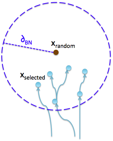
Figure 6: The selection of the best neighbor in BestNear. The best path cost node in $\mathcal{B}(x_{random},\delta_{BN})$ is selected.

Nevertheless, the NAIVE_RANDOM_TREE approach employs a naïve selection strategy, where a node $x_{selected}$ is selected uniformly at random. This has the effect that the resulting method does not have a good convergence rate in finding high-quality solutions as a function of iterations. It is not clear to the authors if a version of the NAIVE_RANDOM_TREE algorithm using an Exploration_First_Selection strategy is asymptotically optimal and most importantly whether it has better convergence rate properties, i.e., whether a method like EST or a version of RRT-Extend that employs MonteCarlo-Prop are asymptotically optimal with good convergence rate. The experimental indications for RRT-Extend with MonteCarlo-Prop are that it does not improve path quality quickly.

Improving Convergence Rate: A solution, however, has been identified to this issue. In particular, the authors propose the use of a Best_First_Selection strategy as a desirable alternative for node selection so as to achieve good convergence to high-quality paths. In this context, best-first means that the node $x_{selected}$ should be chosen so that the method prioritizes nodes that correspond to good quality paths, while also balancing exploration objectives. For instance, one way to achieve this in an RRT-like fashion (described in detail in the consecutive section) is shown in Figure 6, i.e., first sample a random state $x_{random}$ and then among all the nodes on the tree within a certain radius $\delta_{BN}$, select the one that has the best path cost from the root. A similar selection strategy has actually been proposed in the past as a variant of RRT that experimentally exhibited good behavior (Urmson & Simmons, 2003). This previous work, however, did not integrate this selection strategy with the MonteCarlo-Prop procedure and did not show any desirable properties for the resulting algorithm.

The analysis shows that the consideration of a best first strategy together with the random propagation procedure leads to an asymptotically $\delta$-robust near-optimal solution with good convergence rate per iteration. This allows to observe improvement in solution paths over time in practice. Nevertheless, there are additional considerations to take into account when implementing a sampling-based planner. In particular, the asymptotically dominant operation computationally for these methods corresponds to nearest neighbor queries. The implementation of Best_First_Selection described above and in Figure 6 requires the use of a range query that is more expensive than the traditional closest neighbor query in RRT making the individual iteration cost of the proposed solution more expensive. Consequently, the challenge becomes whether this good convergence rate per iteration can be achieved, while also reducing the running time for each iteration.

Balancing Computation Cost with Optimality: The property achieved with the Best_First_Selection strategy is that of asymptotic $\delta$-robust near-optimality. This means that there should be an optimum trajectory $\pi^{*}$ in $\mathbb{X}$ which has $\delta$-robust clearance, as indicated in the problem setup. This property also implies that it is not necessary to keep all samples as nodes in the data structure so as to get arbitrarily close to $\pi^{*}$. It is sufficient to have nodes that are in the vicinity of the path that is defined by its robust clearance $\delta$. Thus, it is possible for a sparse data structure with a finite set of states to sufficiently represent $\mathbb{X}$ as long as it can return $\delta$-similar solutions to all possible optimal trajectories in $\mathbb{X}$.

This allows for a pruning operation, where certain nodes can be forgotten. Which trajectories should a sampling-based planner maintain during its incremental operation and which ones should it prune? The idea is motivated by the same objectives as that of the Best_First_Selection strategy and is illustrated in Figures 7 and 8. The pruning operation should maintain nodes that correspond locally to good paths. For instance, it is possible to evaluate whether a node has the best cost in a local vicinity and prune neighbors with worse cost as long as they do not have children with good path costs in their local neighborhood. Nodes with high path cost in a local neighborhood do not need to be considered again for propagation. There are many different ways to define local neighborhoods. For instance, a grid-based discretization of the space could be defined. In the accompanying implementation and analysis, this work follows an incremental approach of defining visited regions of the state space space as described in Figure 8.

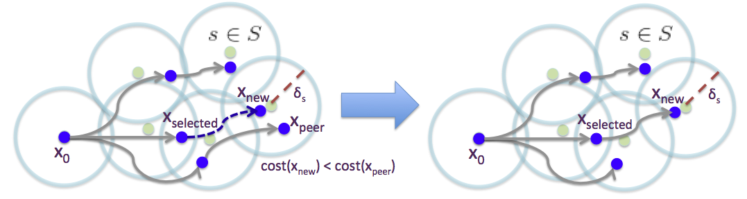
Figure 7: The pruning operation to achieve a sparse data structure that stores asymptotically near-optimal trajectories. Propagation from $x_{selected}$ results to node $x_{new}$, which has a better path cost than a node $x_{peer}$ in its local vicinity. Node $x_{peer}$ is pruned and the newly propagated edge is added to the tree. If $x_{peer}$ had children with the lowest path cost in their neighborhoods, $x_{peer}$ would have remained in the tree but not considered for propagation again. If $x_{new}$ had worse path cost than $x_{peer}$, the old node would have remained in the tree and the last propagation $\overline{x_{selected}\rightarrow x_{new}}$ would have been ignored.

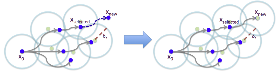
Figure 8: Neighborhoods for pruning are defined based on a set of static witness points $s\in S$, which are generated incrementally. The indicated radii above and in Figure 7 are centered in such witness points. In this figure, the propagation from $x_{selected}$ results in a node $x_{new}$, which is not in the vicinity of an existing witness. In this case, $x_{new}$ is not compared in terms of its path cost with any existing tree node. The edge $\overline{x_{selected}\rightarrow x_{new}}$ is added to the tree and a witness at the location of $x_{new}$ is added to the set of witnesses $S$.

Note that, with high probability, the pruned high-cost nodes would not have been selected for propagation by the best first strategy anyway. In this manner, the pruning operation reinforces the properties of the Best_First_Selection procedure in terms of path quality. The accompanying analysis shows that the specific pruning operation is actually maintaining the convergence properties of the selection strategy. But it also provides significant computational benefits. Since the complexity of all the nearest neighbor queries depends on the number of points in the data structure, having a finite number of nodes, results in queries that have bounded time complexity per iteration. The benefits of sparsity in motion planning have been studied over the last few years by some of the authors (Littlefield et al., 2013; Dobson & Bekris, 2014) and others (Wang et al., 2013; Shaharabani et al., 2013). The discussion section of this paper describes the trade-offs that arise between computational efficiency and the type of guarantee achieved in relation to the requirement for the existence of $\delta$-robust trajectories.

A New Framework: It is now possible to bring together the recommended changes to the original sampling-based tree planners and achieve a new framework for asymptotic near-optimality without a steering function in a computationally efficient way, both in terms of running time and memory requirements. Table 2 is summarizing the differences between the original methods (corresponding to the EXPLORATION_TREE procedure) and the proposed framework for kinodynamic sampling-based planning. The new framework is referred to as SPARSE_BEST_FIRST_TREE in Algorithm 4.

	EXPLORATION_TREE	NAIVE_RANDOM_TREE	SPARSE_BEST_FIRST_TREE
Selection	Exploration_First_Selection	Uniform_Sampling	Best_First_Selection
Propagation	Fixed_Duration_Prop	MonteCarlo-Prop	MonteCarlo-Prop
Pruning	N/A	N/A	Prune_Dominated_Nodes
Properties	Probabilistically Complete (under conditions), Suboptimal but Computationally Efficient, Dense Data Structure	Asymptotically Optimal but Bad Convergence Rate and Impractical, Dense Data Structure	Asymptotically Near-Optimal with Good Convergence Rate and Computationally Efficient with a Sparse Data Structure

Table 2: Outline of differences between the different frameworks in terms of the modules they employ and their properties.

In summary, the three modules of the new framework operate as follows:

• Selection: The new framework still promotes the selection of nodes in under-explored parts of $\mathbb{X}$, as in the original approaches, but within each local region only the nodes that correspond to the best path from the root are selected.

• Propagation: The analysis accompanying this work emphasizes the need to employ a fully random propagation process both in terms of the selected control and duration of propagation, i.e., the MonteCarlo-Prop method, as in EST.

• Pruning: Nodes that are locally dominated in terms of path cost can be removed under certain conditions resulting in a sparse data structure instead of storing infinitely many points.

1 $G=\{\mathbb{V}\leftarrow\{x_{0}\},\mathbb{E}\leftarrow\emptyset\}$;

2 for $N$ iterations do

3       $x_{selected}\leftarrow$ Best_First_Selection( $\mathbb{V},\mathbb{X}$);

4       $x_{new}\leftarrow$ MonteCarlo-Prop( $x_{selected}$, $\mathbb{U}$, $T_{prop}$ );

5      

6      if  CollisionFree$(\overline{x_{selected}\to x_{new}})$ then

7             if  Is_Node_Locally_the_Best( $x_{new}$, $\mathbb{V}$ )  then

8                   $\mathbb{V}\leftarrow\mathbb{V}\cup\{x_{new}\}$;

9                   $\mathbb{E}\leftarrow\mathbb{E}\cup\{\overline{x_{selected}\to x_{new}}\}$;

10                  

11                  Prune_Dominated_Nodes( $x_{new}$, $G$ );

12                  

13            

14      

15return $G(\mathbb{V},\mathbb{E})$;

Algorithm 4 SPARSE_BEST_FIRST_TREE($\mathbb{X}_{f}$, $\mathbb{U}$, $x_{0}$, $T_{prop}$, $N$)

The following section provides an efficient instantiation of the SPARSE_BEST_FIRST_TREE framework, which has been used both in the theoretical analysis and the experimental evaluation of this paper. This algorithm, called STABLE_SPARSE_RRT (SST), provides concrete implementations of the Best_First_Selection, Is_Node_Locally_the_Best and Prune_Dominated_Nodes procedures. The analysis shows that it is asymptotically near-optimal with a good convergence rate and computationally efficient.

The near-optimality property stems from the consideration of $\delta$-robust optimal trajectories. The existence of at least weak $\delta$-robust clearance for optimal trajectories has been considered in the related literature that achieves asymptotic optimality in the kinematic case. To show asymptotic optimality for RRT^∗, one can show that the requirement for the $\delta$ value reduces as the algorithm progresses. The true value $\delta$ depends on the specific problem to be solved and is typically not known beforehand. The way to address this issue is to first assume an arbitrary value for $\delta$ and then repeatedly shrink the value for answering motion planning queries. This is the approach considered here for extending SST into an asymptotically optimal approach SST^∗.

4.2 STABLE_SPARSE_RRT (SST)

Algorithm 5 provides a concrete implementation of the abstract framework of SPARSE_BEST_FIRST_TREE outlined in the previous section and corresponds to one of the proposed algorithms, STABLE_SPARSE_RRT (SST), which is analyzed in the next section.

At a high-level, SST follows the abstract framework. For $N$ iterations, a selection/propagation/pruning procedure is followed. The selection follows the principle of the best first strategy to return an existing node on the tree $x_{selected}$ (line 5). Its concrete implementation is described in detail here. Then MonteCarlo-Prop is called (line 6), which samples a random control and a random duration and then integrates forward the system dynamics according to Eq. 1. If the path $\overline{x_{selected}\rightarrow x_{new}}$ is collision-free (line 7), the new node $x_{new}$ is evaluated on whether is the best node in terms of path cost in a local neighborhood (line 8). If $x_{new}$ is indeed better, it is added to the tree (lines 9-10) and any previous node in the same local vicinity that is dominated, is pruned (line 11).

1 $\mathbb{V}_{active}\leftarrow\{x_{0}\},\mathbb{V}_{inactive}\leftarrow\emptyset$;

2 $G=\{V\leftarrow(\mathbb{V}_{active}\cup\mathbb{V}_{inactive}),\mathbb{E}\leftarrow\emptyset\}$;

3 $s_{0}\leftarrow x_{0}$, $s_{0}.rep=x_{0}$, $S\leftarrow\{s_{0}\}$;

4 for $N$ iterations do

5       $x_{selected}\leftarrow$Best_First_Selection_SST( $\mathbb{X}$, $\mathbb{V}_{active}$, $\delta_{BN}$);

6       $x_{new}\leftarrow$ MonteCarlo-Prop($x_{selected}$, $\mathbb{U}$, $T_{prop}$);

7      

8      if CollisionFree$(\overline{x_{selected}\to x_{new}})$ then

9             if Is_Node_Locally_the_Best_SST($x_{new}$, $S$, $\delta_{s}$) then

10                   $\mathbb{V}_{active}\leftarrow\mathbb{V}_{active}\cup\{x_{new}\}$;

11                   $\mathbb{E}\leftarrow\mathbb{E}\cup\{\overline{x_{selected}\to x_{new}}\}$;

12                   Prune_Dominated_Nodes_SST($x_{new}$, $\mathbb{V}_{active}$, $\mathbb{V}_{inactive}$, $\mathbb{E}$ );

13                  

14            

15      

16return $G$;

Algorithm 5 STABLE_SPARSE_RRT( $\mathbb{X}$, $\mathbb{U}$, $x_{0}$, $T_{prop}$, $N$, $\delta_{BN}$, $\delta_{s}$)

The new aspects of the approach introduced by the concrete implementation are the following:

i) SST requires an additional input parameter $\delta_{BN}$, used in the selection process of the Best_First_Selection_SST procedure shown in Alg. 6, inspired from previous work (Urmson & Simmons, 2003).

ii) SST requires an additional input parameter $\delta_{s}$, used to evaluate whether a newly generated node $x_{new}$ has locally the best path cost in the Is_Node_Locally_the_Best_SST procedure of Alg. 7, useful for pruning.

iii) SST splits the nodes of the tree $\mathbb{V}$ into two subsets: $\mathbb{V}_{active}$ and $\mathbb{V}_{inactive}$. The nodes in $\mathbb{V}_{active}$ correspond to nodes that in a local neighborhood have the best path cost from the root. The nodes $\mathbb{V}_{inactive}$ correspond to dominated nodes in terms of path cost but have children with good path cost in their local neighborhoods and for this reason are maintained on the tree for connectivity purposes. Lines 1 and 2 of Algorithm 5 initialize the sets and the graph data structure $G(\mathbb{V},\mathbb{E})$, which will be returned by the algorithm. Only nodes in $\mathbb{V}_{active}$ are considered for propagation and participate in the Best_First_Selection_SST procedure (line 5). These two sets are updated when a new state $x_{new}$ is generated that dominates its local neighborhood and pruning is performed (lines 9 and 11).

iv) In order to define local neighborhoods, SST uses an auxiliary set of states, called ‘‘witnesses’’ and denoted as $S$. The approach maintains the following invariant with respect to $S$: for every witness $s$ kept in $S$, a single node in the tree will represent that witness (stored in the field $s.rep$ of the corresponding witness), and that node will have the best path cost from the root within a $\delta_{s}$ distance of the witness $s$. All nodes generated within distance $\delta_{s}$ of the witness $s$ with a worse path cost then $s.rep$ are removed from $\mathbb{V}_{active}$, thereby resulting in a sparse data structure. Line 3 of Algorithm 5 initializes the set $S$ to correspond to the root state of the tree, which becomes its own representative. The set $S$ is used by the Is_Node_Locally_the_Best_SST procedure to identify whether the newly generated sample $x_{new}$ is dominating the $\delta_{s}$-neighborhood of its closest witness $s\in S$. The same procedure is responsible for updating the set $S$.

There are two input parameters to SST, $\delta_{BN}$ and $\delta_{s}$. $\delta_{BN}$ influences the number of nodes that are considered when selecting nodes to extend. The larger this parameter is, the more likely that exploration will be ignored and path quality will take precedent. For this reason, care must be taken to not make $\delta_{BN}$ too large. $\delta_{s}$ is the parameter responsible for performing pruning and providing a sparse data structure. As with $\delta_{BN}$, there is a tradeoff with $\delta_{s}$. The larger this parameter is, the more pruning will be performed, which helps computationally but then problems may not be solved if it is not possible to sample inside narrow passages. Given the analysis that follows, these two parameters need to satisfy the relationship specified in the following proposition:

Proposition 13.

The parameters $\delta_{BN}$ and $\delta_{s}$ need to satisfy the following relationship given the robust clearance $\delta$ of the $\delta$-robust feasible motion planning problem that needs to be solved:

$$\delta_{BN}+2\cdot\delta_{s}<\delta$$

.

Figure 9 summarizes the relationship between sets $\mathbb{V}_{active}$, $\mathbb{V}_{inactive}$ and $S$ in the context of the algorithm. The following discussion outlines the implementation of the three individual functions for the best first selection and the pruning operation.

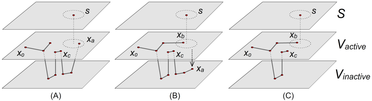
Figure 9: Relation between $S$, $V_{active}$, and $V_{inactive}$. ($A$) A tree and a trajectory $\overline{x_{0}\to x_{c}\to x_{a}}$ where $x_{a}$ is the representative of $s$; Some of the nodes along this path are locally dominated in terms of path cost and exist in the $\mathbb{V}_{inactive}$ set. They remain in the tree, however, because $x_{a}$ is a representative. ($B$) The algorithm extends a new trajectory $\overline{x_{0}\to x_{b}}$ where $x_{b}$ has better cost than $x_{a}$. Then, $x_{a}$ is removed from $V_{active}$ and inserted into $V_{inactive}$. ($C$) The representative of $s$ is now $x_{b}$. The leaf trajectory $\overline{x_{c}\to x_{a}}$ that lies in $\mathbb{V}_{inactive}$ is recursively removed because all of these nodes are dominated and have no longer any children in the active set.

Best First Selection for SST: Algorithm 6 outlines the operation. The method first samples a random point $x_{rand}$ in the state space $\mathbb{X}$ (line 1) and then finds a set of states $X_{near}$ within distance $\delta_{BN}$ of $x_{rand}$ (Line 2). If the set $X_{near}$ is empty, then BestNear defaults to using the nearest neighbor to the random sample as in RRT (line 3). Among the states in $X_{near}$, the procedure will select the vertex that corresponds to the lowest trajectory cost from the root of the tree $x_{0}$ (Line 4).

1 $x_{rand}\leftarrow$ Sample_State($\mathbb{X}$);

2 $X_{near}\leftarrow$Near$(\mathbb{V},x_{rand},\delta_{BN})$;

3 If $X_{near}=\emptyset\$ return Nearest$(\mathbb{V},x_{rand})$;

4 Else return $\arg\min_{x\in X_{near}}cost(x)$;

Algorithm 6 Best_First_Selection_SST($\mathbb{X}$, $\mathbb{V}$, $\delta_{BN}$)

Relative to RRT^∗, this method also uses a neighborhood and tries to propagate a node along the best path from the root. Nevertheless, RRT^∗ propagates the closest node to $x_{rand}$ and then attempts connections between all nodes in $X_{near}$ set to the new state. These steps require multiple calls to a steering function. Here, a near-optimal node in a neighborhood of the random sample is directly selected for propagation, which is possible without a steering function but only using a single forward propagation of the dynamics. A procedure similar to BestNear was presented as a heuristic version of RRT in previous work (Urmson & Simmons, 2003). Here it is formally analyzed to show its mathematical guarantees in terms of path quality and convergence properties.

Pruning in SST: Algorithm 7 describes the conditions under which the newly propagated node $x_{new}$ is considered for addition to the tree. First, the closest witness $s_{new}$ to $x_{new}$ from the set $S$ is computed (line 1). If the closest witness is more than $\delta_{s}$ away, then the sample $x_{new}$ becomes a new witness itself (lines 2-5). The representative of the witness $s$ is stored in the variable $x_{peer}$ (line 6). Then the new sample $x_{new}$ is considered viable for addition in the tree, if at least one of two conditions holds (line 7): i) there is no representative $x_{peer}$, i.e., the sample $x_{new}$ was just added as a witness or ii) the cost of the new sample $cost(x_{new})$ is less than the cost of the witness’ representative $cost(x_{peer})$. If the function returns true, node $x_{new}$ is added to the tree and the active set of nodes $\mathbb{V}_{active}$. If not, then the last propagation is ignored.

1 $s_{new}\leftarrow$ Nearest($S$,$x_{new}$);

2 if $||x_{new}-s_{new}||>\delta_{s}$ then

3       $S\leftarrow S\cup\{x_{new}\}$;

4       $s_{new}\leftarrow x_{new}$;

5       $s_{new}.rep\leftarrow NULL$;

6      

7$x_{peer}\leftarrow s_{new}.rep$;

8 if $x_{peer}==NULL$ or cost($x_{new}$) $\ <\$cost($x_{peer}$) then

9       return true;

10      

11return false;

Algorithm 7 Is_Node_Locally_the_Best_SST($x_{new}$, $S$, $\delta_{s}$)

Algorithm 8 describes the pruning process of dominated nodes when SST is adding node $x_{new}$. First the witness $s_{new}$ of the new node and its previous representative $x_{peer}$ are found (lines 1-2). The previous representative, which is dominated by $x_{new}$ in terms of path cost, is removed from the active set of nodes $\mathbb{V}_{active}$ and is added to the inactive one $\mathbb{V}_{inactive}$ (lines 4-5). Then, $x_{new}$ replaces $x_{peer}$ as the representative of its closest witness $s$ (line 6). If $x_{peer}$ is a leaf node, then it can also safely be removed from the tree (lines 7-11). The removal of $x_{peer}$ may cause a cascading effect for its parents, if they were already in the inactive set $\mathbb{V}_{inactive}$ and the only reason they were maintained in the tree was because they were leading to $x_{peer}$ (lines 7-11). This cascading effect is also illustrated in Figure 9 (C).

1 $s_{new}\leftarrow$ Nearest($S$,$x_{new}$);

2 $x_{peer}\leftarrow s_{new}.rep$;

3 if $x_{peer}!=NULL$ then

4       $\mathbb{V}_{active}\leftarrow\mathbb{V}_{active}\setminus\ \{x_{peer}\}$;

5       $\mathbb{V}_{inactive}\leftarrow\mathbb{V}_{inactive}\cup\ \{x_{peer}\}$;

6      

7$s_{new}.rep\leftarrow x_{new}$;

8 while  $x_{peer}!=NULL$  and IsLeaf $(x_{peer})$  and $x_{peer}\in\mathbb{V}_{inactive}$  do

9       $x_{parent}\leftarrow$Parent$(x_{peer})$;

10       $\mathbb{E}\leftarrow\mathbb{E}\setminus\{\overline{x_{parent}\to x_{peer}}\}$;

11       $\mathbb{V}_{inactive}\leftarrow\mathbb{V}_{inactive}\setminus\ \{x_{peer}\}$;

12       $x_{peer}\leftarrow x_{parent}$;

13      

Algorithm 8 Prune_Dominated_Nodes_SST($x_{new}$, $\mathbb{V}_{active}$, $\mathbb{V}_{inactive}$, $\mathbb{E}$ )

Implementation Guidelines: The pseudocode provided here for SST contains certain inefficiencies to simplify its description, which should be avoided in an actual implementation.

In particular, in line 7 of the STABLE_SPARSE_RRT procedure, the trajectory $\overline{x_{selected}\rightarrow x_{new}}$ is collision checked and then the algorithm evaluates whether $x_{new}$ is useful to be added to the tree. Typically, the operations for evaluating whether $x_{new}$ is useful (nearest neighbor queries, data structure management and mathematical comparisons) are faster than collision checking a trajectory. Consequently, it is computationally advantageous if the check for whether $x_{new}$ is useful, is performed before the collision checking of $\overline{x_{selected}\rightarrow x_{new}}$. This is possible if the underlying moving system is modeled through a set of state update equations of the form of Equation 1. If, however, the moving system is a physically simulated one, then it is not possible to figure out what is the actual final state $x_{new}$ of the propagated trajectory, without first performing collision checking. Thus, in the case of a physically simulated system, the description of the algorithm is closer to the implementation.

Another issue relates to the first two lines of Algorithm 8, which find the closest witness to the new node $x_{new}$ and its previous representative. These operations have actually already taken place in Algorithm 7 (lines 1 and 6 respectively). An efficient implementation would avoid the second call to a nearest neighbor query and reuse the information regarding the closest witness to node $x_{new}$ between the two algorithms.

4.3 STABLE_SPARSE-RRT^∗ (SST*)

SST is providing only asymptotic $\delta$-robust near-optimality. Asymptotic optimality cannot be achieved by SST directly primarily due to the fixed sized pruning operation employed. The solution to this is to slowly reduce the radii $\delta_{BN}$ and $\delta_{s}$ employed by the algorithm eventually converging to iterations that are similar to the NAIVE_RANDOM_TREE approach. The key to SST^∗, which is provided in Algorithm 9, is to make sure that the rate of reducing the pruning is slow enough to achieve an anytime behavior, where initial solutions are found for large radii and then they are improved. As the radii decrease, the algorithm is able to discover new homotopic classes that correspond to narrow passages where solution trajectories have reduced clearance.

1 $j\leftarrow 0$; $N\leftarrow N_{0}$;

2 $\delta_{s}\leftarrow\delta_{s,0}$; $\delta_{BN}\leftarrow\delta_{BN,0}$;

3 while true do

4       $SST(\mathbb{X},\mathbb{U},x_{0},T_{prop},N,\delta_{BN},\delta_{s})$;

5       $\delta_{s}\leftarrow\xi\cdot\delta_{s}$; $\delta_{BN}\leftarrow\xi\cdot\delta_{BN}$;

6       $j\leftarrow j+1$;

7       $N\leftarrow(1+\log j)\cdot\xi^{-(d+l+1)j}\cdot N_{0}$;

Algorithm 9 SST^∗( $\mathbb{X}$, $\mathbb{U}$, $x_{0}$, $T_{prop}$, $N_{0}$, $\delta_{BN,0}$, $\delta_{s,0}$, $\xi$ )

SST^∗ provides a schedule for reducing the two radii parameters to SST, $\delta_{BN}$ and $\delta_{s}$ over time. It receives as input an additional parameter $\xi$, which is used to decrease the radii $\delta_{BN}$ and $\delta_{s}$ over consecutive calls to SST (note that $d$ and $l$ are the dimensionalities of the state and control spaces respectively). This, in effect, makes pruning more difficult to occur, turns the selection procedure more towards an exploration objective instead of a best-first strategy and increases the number of nodes in the data structure. As the number of iterations approaches infinity, pruning will no longer be performed, the selection process works in a uniformly at random manner and all collision-free states will be generated.

Alg. 9 is a meta-algorithm that repeatedly calls SST as a building block. In the above call, SST is assumed to be operating on the same graph data structure $G$ over repeated calls. It is possible to take advantage of previously generated versions of the graph data structures with some additional considerations, e.g., instead of clearing out all states in $V_{active}$ from previous iterations, one can carefully modify the pruning procedure to take advantages of the existing $V_{active}$ set given the updated radii.

4.4 Nearest Neighbor Data Structure

The implementation of SST imposes certain technical requirements from the underlying nearest neighbor data structure that are not typical for existing sampling-based motion planners. In particular, given the pruning operation, it is necessary to have an efficient implementation of deletion from the nearest neighbor data structure. In most nearest neighbor structures, a removal of a node will cause the entire data structure to be frequently rebuilt, severely increasing run times.

1 $V_{rand}\leftarrow$ Sample_Random_Vertices$(\mathbb{G}.\mathbb{V})$;

2 $v_{min}\leftarrow\underset{x\in V_{rand}}{\operatorname{arg}\,\operatorname{min}}\;||x-v||$;

3 repeat

4       $Nodes\leftarrow{\tt Neighbors}(v_{min})\cup\{v_{min}\}$;

5       $v_{min}\leftarrow\underset{x\in Nodes}{\operatorname{arg}\,\operatorname{min}}\;||x-v||$;

6      

7until $v_{min}$ unchanged;

8return $v_{min}$;

Algorithm 10 Find_Closest($\mathbb{G}$,$v$)

The goal here is to describe a simple idea for performing approximate nearest neighbor search using a graph structure $\mathbb{G}$ that stores the nodes of the tree and on its edges stores distances between them according to $d_{x}(\cdot,\cdot)$. This approach builds on top of ideas from random graph theory. Graphs are conducive to easy removal, but some overhead is placed in node addition to maintain this data structure incrementally.

The key operation is finding the closest node in a graph, which is performed by following a hill climbing approach shown in Algorithm 10. A random set of nodes is first sampled from the existing structure, proportional to $\sqrt{\|\mathbb{V}\|}$ (line 1). From this set of nodes, the closest node to the query node $v$ is determined by applying linear search according to $d_{x}(\cdot,\cdot)$ (line 2). From the closest node, a hill climbing process is performed by searching the local neighborhood of the closest node on the graph to identify whether there are nodes that are closer to the query one (line 3-6). Once no closer nodes can be found, the locally best node is returned (line 7).

On top of this operation, it is also possible to define a way for approximately finding the $k$-closest nodes or the nodes that are within a certain radius $\delta$.

1 $v_{min}\leftarrow{\tt FindClosest}(\mathbb{G},v)$;

2 $K_{near}\leftarrow\{v_{min}\}$;

3 repeat

4       $Nodes\leftarrow{\tt Neighbors}(K_{near})$;

5       $K_{near}\leftarrow K_{near}\cup Nodes$;

6       $K_{near}\leftarrow$ Keep_K_Closest($K_{near}$,$v$,$k$);

7      

8until $K_{near}$ unchanged;

9return $K_{near}$;

Algorithm 11 Find_K_Close($\mathbb{G}$,$v$,$k$)

The idea in both cases is to start from the closest node by calling Algorithm 10. Then, each corresponding method searches the local neighborhoods of the discovered nodes (initially just the closest node) for either the $k$-closest ones or those nodes that are within $\delta$ distance. The methods iterate by searching locally until there is no change in the list.

1 $\mathbb{G}.\mathbb{V}\leftarrow\mathbb{G}.\mathbb{V}\cup\{v\}$;

2 $K_{near}\leftarrow$FindKClose( $\mathbb{G}$, $v$, $k\propto\log(|\mathbb{G}.\mathbb{V}|)$ );

3 foreach $x\in K_{near}$ do

4       $\mathbb{G}.\mathbb{E}\leftarrow\mathbb{G}.\mathbb{E}\cup\{(v,x)\}\cup\{(x,v)\}$;

5      

6return $\mathbb{G}$;

Algorithm 12 AddNode($\mathbb{G}$,$v$)

The process of adding nodes to the nearest neighbor data structure is shown in Algorithm 12. It is achieved by first finding the $k$ closest nodes and then adding edges to them. The number $k$ should be at least a logarithmic number of nodes as a function of the total number of nodes to ensure the graph is connected (similar to PRM^∗).

1 foreach $\{e\in\mathbb{G}.\mathbb{E}\ |\ e.source=v\ \|\ e.target=v\}$ do

2       $\mathbb{G}.\mathbb{E}\leftarrow\mathbb{G}.\mathbb{E}\setminus{e}$;

3      

4$\mathbb{G}.\mathbb{V}\leftarrow\mathbb{G}.\mathbb{V}\setminus{v}$;

5 return $\mathbb{G}$;

Algorithm 13 RemoveNode($\mathbb{G}$,$v$)

The reason for using a graph data structure for the nearest neighbor operations is the ease of removal shown in Algorithm 13. Most implementations of graph data structures provide such a primitive that is typically quite fast. This can be sped up even more if a link to the nearest neighbor graph node is kept with the tree node allowing for constant time removal.

5 Analysis

In this section, arguments for the proposed framework are provided. Sec. 5.1 begins by discussing the requirements of MonteCarlo-Prop and what properties this primitive provides. Then, in Sec. 5.2, an analysis of the NAIVE_RANDOM_TREE approach is outlined, showing that this algorithm can achieve asymptotic optimality. To address the poor convergence rate of that approach, the properties of using the best-first selection strategy are detailed in Sec. 5.3. Finally, in order to introduce the pruning operation, properties of SST and SST^∗ are studied in Sec. 5.4 and 5.5.

5.1 Properties of MonteCarlo-Prop

The MonteCarlo-Prop procedure is a simple primitive for generating random controls, but provides desirable properties in the context of achieving asymptotic optimality properties for systems without access to a steering function. This section aims to illustrate these desirable properties, given the assumptions from Section 3. Much of the following analysis will use these results to prove the probabilistic completeness and asymptotic near-optimality properties of SST and asymptotic optimality of SST^∗. These algorithms are using MonteCarlo-Prop for generating random controls.

The analysis first considers a $\delta$-robust optimal path for a specific planning query, which is guaranteed to exist for the specified problem setup. For such a path, consider a covering ball sequence (an illustration is shown in Fig. 10(left)):

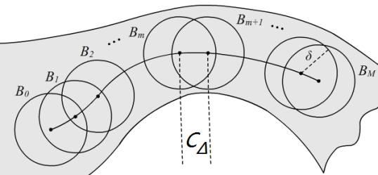
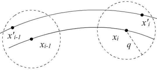
Figure 10: (left) An example of a covering ball sequence over a given trajectory of radius $\delta$, where each ball is placed so that its center has cost $C_{\Delta}$ from the previous ball center. (right) The states involved in the arguments regarding the properties of random local propagation.

Definition 14.

(Covering Balls) Given a trajectory $\pi(t)$: $[0,t_{\pi}]\rightarrow\mathbb{X}_{f}$, robust clearance $\delta\in R^{+}$, and a cost value $C_{\Delta}>0$, the set of covering balls $\mathbb{B}$($\pi(t)$, $\delta$, $C_{\Delta}$) is defined as a set of $M+1$ hyper-balls: {$\mathcal{B}_{\delta}(x_{0})$, $\mathcal{B}_{\delta}(x_{1})$, …, $\mathcal{B}_{\delta}(x_{M})$} of radius $\delta$, where $x_{i}$ are defined such that Cost($\overline{x_{i}\to x_{i+1}}$)$=C_{\Delta}\$ for $i=0,1,...,M-1$.

Note that Assumption 11 about the Lipschitz continuity of the cost function and Definition 14 imply that for any given trajectory $\pi$, where $cost(\pi)=C$, and a given duration $T>0$, it is possible to define a set of covering balls $\mathbb{B}$($\pi(t)$, $\delta$, $C_{\Delta}$) for some $C_{\Delta}>0$, where the centers $x_{i}$ of those balls occur at time $t_{i}$ of the executed trajectory. Since for the given problem setup, the cost function is non-decreasing along the trajectory and non-degenerate, every segment of $\pi$ will have a positive cost value.

The covering ball sequence, in conjunction with the following theorem, provide a basis for the remaining arguments. In particular, much of the arguments presented in the rest of Section 5 will consider this covering ball sequence and the fact that the proposed algorithm can generate a path, which exists entirely in this covering ball sequence. Once the generation of such a path asymptotically is proven, its properties in terms of path quality relatively to the $\delta$-robust optimal path will be examined.

Theorem 15.

For two trajectories $\pi,\pi^{\prime}$ and any period $T\geq 0$, so that $\pi(0)=\pi^{\prime}(0)=x_{0}$ and $\Delta u=\sup_{t}(||u(t)-u^{\prime}(t)||)$:

$$||\pi^{\prime}(T)-\pi(T)||<K_{u}\cdot T\cdot e^{K_{x}\cdot T}\cdot\Delta u.$$

Intuitively, this theorem guarantees that for two trajectories starting from the same state, the distance between their end states, in the worst case, is bounded by a function of the difference of their control vectors. This theorem examines the worst case, and as a result, the exact bound value is conservative. The proof can be found in Appendix B. From this theorem, the following corollary is immediate.

Corollary 16.

For two trajectories $\pi$ and $\pi^{\prime}$ such that $\pi(0)=\pi^{\prime}(0)=x_{0}$ and $\Delta u=\sup_{t}(||u(t),u^{\prime}(t)||)$: $\lim_{\Delta u\rightarrow 0^{+}}||\pi(T)-\pi^{\prime}(T)||=0$ for any period $T\geq 0$.

Corollary 16 is the reason why MonteCarlo-Prop can be used to replace a Steering function. By having the opportunity to continuously sample control vectors and propagate them forward from an individual state $x_{0}$, one can get arbitrarily close to the optimal control vector, i.e., producing a $\delta$-similar trajectory, where the $\delta$ value can get arbitrarily small.

The following theorem guarantees that the probability of generating $\delta$-similar trajectories is nonzero when starting from a different initial point inside a $\delta$-ball, allowing situations similar to Figure 10 (right) to occur. This property shows why MonteCarlo-Prop is a valid propagation primitive for use in an asymptotically optimal motion planner.

Theorem 17.

Given a trajectory $\pi$ of duration $t_{\pi}$, the success probability for MonteCarlo-Prop to generate a $\delta$-similar trajectory $\pi^{\prime}$ to $\pi$ when called from an input state $\pi^{\prime}(0)\in\mathcal{B}_{\delta}(\pi(0))$ and for a propagation duration $t_{\pi^{\prime}}=T_{prop}>t_{\pi}$ is lower bounded by a positive value $\rho_{\delta}>0$.

Proof: As in Figure 11, consider that the start of trajectory $\pi$ is $\pi(0)=x_{i-1}$, while its end is $\pi(t_{\pi})=x_{i}$. Similarly for $\pi^{\prime}$: $\pi^{\prime}(0)=x^{\prime}_{i-1}$ and $\pi^{\prime}(t_{\pi^{\prime}})=x_{i}^{\prime}$. From Lemma 6 regarding the existence of dynamic clearance we have the following: regardless of where $x^{\prime}_{i-1}$ is located inside $\mathcal{B}_{\delta}(x_{i-1})$, there must exist a $\delta$-similar trajectory $\pi^{\prime}$ to $\pi$ starting at $x^{\prime}_{i-1}$ and ending at $x_{i}^{\prime}$. Therefore, if the reachable set of nodes $A_{T_{prop}}$ from $x_{i-1}^{\prime}$ is considered, it must be true that $\mathcal{B}_{\delta}(x_{i})\subseteq A_{T_{prop}}$.

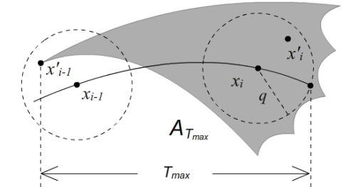
Figure 11: An illustration of the local reachability set for $x_{i-1}^{\prime}$. Gray region $A_{T_{max}}=A_{T_{prop}}$ denotes the set of states that is reachable from $x_{i-1}^{\prime}$ within duration $[0,t_{\pi^{\prime}}]$.

In other words, $A_{T_{prop}}$ has the same dimensionality $d$ as the state space (Assumption 5), as in in Fig. 11. The goal is to determine a probability $\rho$ that trajectory $\pi^{\prime}$ will have an endpoint in $\mathcal{B}_{\delta}(\pi(t_{\pi}))$.

Consider Fig. 12 (left). Given a $\lambda\in(0,1)$, construct a ball region $b=\mathcal{B}_{\lambda\delta}(x_{b})$, such that the center state $x_{b}\in\pi(t)$ and $b\subset\mathcal{B}_{\delta}(x_{i})$. Let $\Lambda_{\delta}$ denote the union of all such $b$ regions. Clearly, all of $x_{b}$ form a segment of trajectory $\pi(t)$. Let $T_{\delta}$ denote the time duration of this trajectory segment. For any state $x_{b}$, there must exist a $\delta$-similar to $\pi$ trajectory $\pi_{b}=\overline{x_{i-1}^{\prime}\to x_{b}}$, due to Lemma 6.

Recall that MonteCarlo-Prop samples a duration for integration, and then, samples a control vector in $\Upsilon$. The probability to sample a duration $t_{\pi_{b}}$ for $\pi_{b}$ so that it reaches the region $\Lambda\delta$ is $T_{\delta}/T_{prop}$.

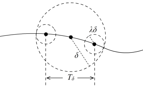
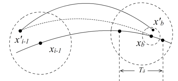
Figure 12: (left) A constructed segment of trajectory $\pi$ of duration $T_{\delta}$. (right) The dotted curve illustrates the existence of a trajectory, and the solid curve above it illustrates one possible edge that is created by MonteCarlo-Prop.

Since the trajectory segment exists, it corresponds to a control vector $u_{m}\in\Upsilon$. MonteCarlo-Prop only needs to sample a control vector $u_{m}^{\prime}$, such that it is close to $u_{m}$ and results in a $\delta$-similar trajectory. Then Theorem 15 guarantees that MonteCarlo-Prop can generate trajectory $\pi_{b}^{\prime}=\overline{x_{i-1}^{\prime}\to x_{b}^{\prime}}$, which has bounded ‘‘spatial difference’’ from $\overline{x_{i-1}^{\prime}\to x_{b}}$. And both of them have exactly the same duration of $t_{\pi_{b}}$ (see Fig. 12 (right) for an illustration). More formally, given the ‘‘spatial difference’’ $\lambda\delta$, if MonteCarlo-Prop samples a control vector $u_{m}^{\prime}$ such that:

$$||u_{m}^{\prime}-u_{m}||\leq\frac{\lambda\delta}{K_{u}\cdot T_{prop}\cdot e^{K_{x}\cdot T_{prop}}}\ \ \ \ \ \ \Rightarrow\ \ \ \ \ \ ||x_{b}-x_{b}^{\prime}||<\lambda\delta.$$

Therefore, starting from state $x_{i-1}^{\prime}$, with propagation parameter $T_{prop}$, MonteCarlo-Prop generates a $\delta$-similar trajectory $\overline{x_{i-1}^{\prime}\to x_{b}^{\prime}}$ to $\overline{x_{i-1}\to x_{i}}$ with probability at least

$$\rho_{\delta}=\frac{T_{\delta}}{T_{prop}}\cdot\frac{\zeta\cdot(\frac{\lambda\delta}{K_{u}\cdot T_{prop}\cdot e^{K_{x}\cdot T_{prop}}})^{w}}{\mu(U_{m})}>0.$$

$\blacksquare$

This theorem guarantees that the maximum ‘‘spatial difference’’ between $\pi(t)$ and $\pi^{\prime}(t)$, within time $T$, can be bounded and the bound is proportional to the maximum difference of their control vectors. This duration bound also implies a cost bound, which will be leveraged by the following theorems.

5.2 Naive Algorithm: Already Asymptotically Optimal

This section considers the impractical sampling-based tree algorithm outlined in Algorithm 2, which does not employ a steering function. Instead, it selects uniformly at random a reachable state in the existing tree and applies random propagation to extend it. The following discussion argues that this algorithm eventually generates trajectories $\delta$-similar to optimal ones. The general idea is to prove by induction that a sequence of trajectories between the covering balls of an optimal trajectory can be generated. This proof shows probabilistic completeness. Then, from the properties of MonteCarlo-Prop, the quality of the trajectory generated in this manner is examined. Finally, if the radius of the covering-ball sequence tends toward zero, asymptotic optimality is achieved.

Consider an optimal trajectory $\pi^{\ast}$ and its covering ball sequence $\mathbb{B}$($\pi^{\ast}(t)$, $\delta$, $C_{\Delta}$). Let $A_{k}^{(n)}$ denote the event that at the $n^{th}$ iteration of $ALG$, a $\delta$-similar trajectory $\pi$ to the $k^{th}$ segment of the optimal sub-trajectory $\overline{x_{k-1}^{\ast}\to x_{k}^{\ast}}$ is generated, such that $\pi(0)\in\mathcal{B}_{\delta}(x_{k-1}^{\ast})$ and $\pi(t_{\pi})\in\mathcal{B}_{\delta}(x^{\ast}_{k})$. Then, let $E_{k}^{(n)}$ denote the event that from iteration $1$ to $n$, an algorithm generates at least one such trajectory, thereby expressing whether an event $A_{k}^{(n)}$ has occurred. The following theorems reason about the value of $E_{k}^{(\infty)}$ where $k$ is the number of segments in $\pi^{\ast}$ resulting from the choice of $T_{prop}$.

Theorem 18.

NAIVE_RANDOM_TREE will eventually generate a $\delta$-similar trajectory to an optimal one for any robust clearance $\delta>0$.

The proof of Theorem 18 is in Appendix C. From this theorem, the following is true.

Corollary 19.

NAIVE_RANDOM_TREE is probabilistically complete.

Theorem 20.

NAIVE_RANDOM_TREE is asymptotically optimal.

The proof of Theorem 20 is in Appendix D and shows it is possible to achieve asymptotic optimality in a rather naïve way. This approach is impractical to use however. Consider the rate of convergence for the probability $\mathbb{P}(E_{k}^{(n)})$ where $k$ denotes the $k^{th}$ ball and $n$ is the number of iterations. Given Theorem 18, $\mathbb{P}(E_{k}^{(n)})$ converges to 1. But the following is also true.

Theorem 21.

For the worst case, the $k^{th}$ segments of the trajectory returned by NAIVE_RANDOM_TREE converges logarithmically to the near optimal solution, i.e., $\lim_{n\to\infty}\frac{|\mathbb{P}(E_{k}^{(n+2)})-\mathbb{P}(E_{k}^{(n+1)})|}{|\mathbb{P}(E_{k}^{(n+1)})-\mathbb{P}(E_{k}^{(n)})|}=1.$

The significance of Theorem 21 (proven in Appendix E) comes from the realization that expecting to generate a $\delta$-similar trajectory segment to an optimal trajectory $\pi^{\ast}$ requires an exponential number of iterations with this approach. This can also be illustrated in the following way. In the NAIVE_RANDOM_TREE approach, as in RRT-Connect, each vertex in $V$ has unbounded degree asymptotically.

Theorem 22.

For any state $x_{i}\in V$, such that $x_{i}$ is added into $V$ at iteration $i$, NAIVE_RANDOM_TREE will select $x_{i}$ to be propagated infinitely often as the execution time goes to infinity.

$$\mathbb{P}(\limsup_{n\to\infty}\{x_{i}\text{ is selected}\})=1.$$

Theorem 22 (proven in Appendix F) indicates that NAIVE_RANDOM_TREE will attempt an infinite number of propagations from each node, and the duration of the propagation does not decrease, unlike in RRT-Connect where the expected length of new branches converge to 0 (Karaman & Frazzoli, 2011). The assumption of Lipschitz continuity of the system is enough to guarantee optimality. Due to this reason, NAIVE_RANDOM_TREE is trivially asymptotically optimal.

Another way to reason about the speed of convergence is the following. Let $p$ be the probability of an event to happen. The expected number of independent trials for that event to happen is $1/p$. Then, the probability of such an event happening converges to and is always greater than $1-e^{-1}\approx 63.21\%$, after $1/p$ independent trials, as $p\to 0$ (Grimmett & Stirzaker, 2001). Consider event $A_{1}$ from the previous discussion (the event of generating the first $\delta$-similar trajectory segment to an optimum one at any particular iteration) and recall that the success probability of the MonteCarlo-Prop function is $\rho$. If $x_{0}$ is selected for MonteCarlo-Prop, then the probability of $\mathbb{P}(A_{1}|\{x_{0}\text{ is selected}\})=\rho$. Then the ‘‘expected number’’ of times we need to select $x_{0}$ for $A_{1}$ to happen is $1/{\rho}$. The expected number of times that $x_{0}$ is selected after $n$ iterations is $\sum_{i=1}^{n}\frac{1}{i}$. This yields the following expression for sufficiently large $n$: $\frac{1}{\rho}=\sum_{i=1}^{n}\frac{1}{i}\approx ln(n)+c_{\gamma}$ where $c_{\gamma}$ is the Euler-Mascheroni constant, which yields: $n\approx e^{(\rho^{-1}-c_{\gamma})}.$ Therefore, in order even for event $E_{1}$ (event of $A_{1}$ happening at least once ) to happen with approximately $1-e^{-1}$ probability for small $\rho$ values, the expected number of iterations is exponential to the reciprocal of the success probability $\rho$ of the MonteCarlo-Prop function. This implies intractability. For efficiency purposes it is necessary to have methods where $n$ does not depend exponentially to $\frac{1}{\rho}$.

5.3 Using BestNear: Improving Convergence Rate

A computationally efficient alternative to NAIVE_RANDOM_TREE for finding a path, if one exists, is referred to here as RRT-BestNear, which works like NAIVE_RANDOM_TREE but switches line 3 in Algorithm 2 with the procedure in Algorithm 6. An important observation from the complexity discussion for NAIVE_RANDOM_TREE is that the exponential term arises from the use of uniform random sampling for selection among the existing nodes. By not using any path cost information when performing selection, the likelihood of generating good trajectories becomes very low, even if it is still non-zero.

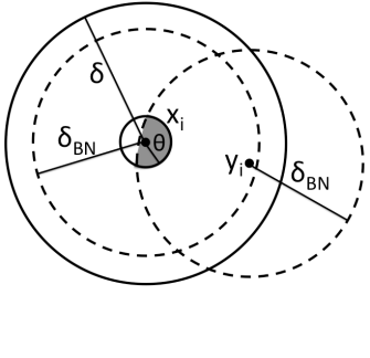
Figure 13: (left) Illustration of different trajectories generated by MonteCarlo-Prop inside the covering balls $\mathbb{B}$($\pi^{\ast}$,$\delta$,$C_{\Delta}$). Many trajectories may enter these balls, but may not be $\delta$-similar to the optimal one. (right) Sampling $x_{rand}$ in the gray region guarantees that a node $z_{i}\in\mathcal{B}_{\delta}(x_{i})$ is selected for propagation so that either $z_{i}=y_{i}$ or $cost(z_{i})<cost(y_{i})$.

The analysis of RRT-BestNear involves similar event constructions as in the previous section: $A_{k}^{(n)}$ and $E_{k}^{(n)}$ are defined as in the previous section, except the endpoint of the trajectory segment generated must be in $\mathcal{B}_{\delta_{BN}}(x_{k}^{\ast})$. The propagation from MonteCarlo-Prop still has positive probability of occurring, but is different from $\rho_{\delta}$. The changed probability for MonteCarlo-Prop to generate such a trajectory is defined as $\rho_{\delta\to\delta_{BN}}$ The probabilities of these events will also change due to the new selection process and more constrained propagation requirements. It must be shown that nodes that have good quality should have a positive probability of selection. Consider the selection mechanism BestNear in the context of Figure 13.

Lemma 23.

Assuming uniform sampling in the Sample function of BestNear, if $\exists\ x$ s.t. $x\in\mathcal{B}_{\delta_{BN}}(x_{i}^{\ast})$ at iteration $n$, then the probability that BestNear selects for propagation a node $x^{\prime}\in\mathcal{B}_{\delta}(x_{i}^{\ast})$ can be lower bounded by a positive constant $\gamma$ for every $n^{\prime}>n$.

Proof: Consider the case that a random sample $x_{rand}$ is placed at the intersection of a small ball of radius $\theta=\delta-\delta_{BN}$ (guaranteed positive from Proposition 13), and of a $\delta_{BN}$-radius ball centered at a state $y_{i}\in\mathcal{B}_{\delta_{BN}}(x_{i})$ that was generated during an iteration of an algorithm. State $y_{i}$ exists with probability $\mathbb{P}(E_{k}^{(n)})$. In other words, if $x_{rand}\in\mathcal{B}_{\theta}(x_{i})\cap\mathcal{B}_{\delta_{BN}}(y_{i})$, then $y_{i}$ will always be considered by BestNear because $y_{i}$ will always be within $\delta_{BN}$ distance of a random sample there. The small circle is defined so that the $\delta_{BN}$ ball of $x_{rand}$ can only reach states in $\mathcal{B}_{\delta}(x_{i})$. It is also required that $x_{rand}$ is in the $\delta_{BN}$-radius ball centered at $y_{i}$, so that at least one node in $\mathcal{B}_{\delta}(x_{i})$ is guaranteed to be returned. Thus, the probability the algorithm select for propagation a node $x^{\prime}\in\mathcal{B}_{\delta}(x_{i}^{\ast})$ can be lower bounded by the following expression:

$$\gamma=\frac{\mu(\mathcal{B}_{\theta}(x_{i})\cap\mathcal{B}_{\delta_{BN}}(x^{\prime}))}{\mu(\mathbb{X}_{f})}>0\vspace{-0.1in}$$

$\blacksquare$

With Theorem 17 and Lemma 23, both the selection and propagation probabilities are positive and it is possible to argue probabilistic completeness of RRT-BestNear. The full proof is provided in Appendix G.:

Theorem 24.

RRT-BestNear will eventually generate a $\delta$-similar trajectory to any optimal trajectory.

The proof of asymptotic $\delta$-robust near-optimality follows directly from Theorem. 24, the Lipschitz continuity, additivity, and monotonicity of the cost function (Assumption 11). Theorem 24 is already examining the generation of a $\delta$-similar trajectory to $\pi^{\ast}$, but the bound on the cost needs to be calculated (as is constructed in Appendix H).

Theorem 25.

RRT-BestNear is asymptotically $\delta$-robustly near-optimal.

The addition of BestNear was introduced to address the convergence rate issues of NAIVE_RANDOM_TREE. Theorem 26 quantifies this convergence rate.

Theorem 26.

For the worst case, the $k^{th}$ segment of the trajectory returned by RRT-BestNear converges linearly to the near optimal solution, i.e, $\lim_{n\to\infty}\frac{|\mathbb{P}(E_{k}^{(n+1)})-1|}{|\mathbb{P}(E_{k}^{(n)})-1|}=(1-\gamma\rho_{\delta\to\delta_{BN}})\in(0,1).$

Proof: Applying the boundary condition of Equation 28, consider the ratio of the probabilities between iteration $n+1$ and $n$.

$$\frac{|\mathbb{P}(E_{k}^{(n+1)})-1|}{|\mathbb{P}(E_{k}^{(n)})-1|}=\frac{\prod_{j=1}^{n+1}(1-\mathbb{P}(E_{k-1}^{(j)})\cdot\gamma\rho_{\delta\to\delta_{BN}})}{\prod_{j=1}^{n}(1-\mathbb{P}(E_{k-1}^{(j)})\cdot\gamma\rho_{\delta\to\delta_{BN}})}=1-\mathbb{P}(E_{k-1}^{(n+1)})\cdot\gamma\rho_{\delta\to\delta_{BN}}$$

Taking $\lim_{n\to\infty}$, and given Theorem 24 such that $\lim_{n\to\infty}\mathbb{P}(E_{k-1}^{(n+1)})=1$, the following holds:

$$\lim_{n\to\infty}\frac{|\mathbb{P}(E_{k}^{(n+1)})-1|}{|\mathbb{P}(E_{k}^{(n)})-1|}=\lim_{n\to\infty}(1-\mathbb{P}(E_{k-1}^{(n+1)})\cdot\gamma\rho_{\delta\to\delta_{BN}})=1-\gamma\rho_{\delta\to\delta_{BN}}\in(0,1).\ \ \ \ \ \ \ \hfill\blacksquare$$

Theorem 26 states that RRT-BestNear converges linearly to near optimal solutions. Recall that the NAIVE_RANDOM_TREE approach converges logarithmically (sub-linearly). This difference indicates that RRT-BestNear converges significantly faster than NAIVE_RANDOM_TREE. Now consider the expected number of iterations, i.e. the iterations needed to return a near-optimal trajectory with a certain probability. Specifically, the convergence rate depends on the difficulty level of the kinodynamic planning problem, which is measured by the probability $\rho_{\delta\to\delta_{BN}}$ of successfully generating a $\delta$-similar trajectory segment connecting two covering balls.

Recall that the expected number of iterations for $E_{1}$ to succeed for NAIVE_RANDOM_TREE was $n\approx e^{c_{\gamma}}\cdot e^{(\rho^{-1})}$. In the case of RRT-BestNear for event $E_{1}$, this expected number of iterations is $\frac{1}{1-e^{-1}}\cdot\frac{1}{\gamma\rho_{\delta\to\delta_{BN}}}$. This is a significant improvement already for event $E_{1}$ (though providing a weaker near-optimality guarantee). For the cases of $E_{k}$, ($k>1$), the expected number of iterations for RRT-BestNear linearly depends on the length of the optimal trajectory. While for NAIVE_RANDOM_TREE, it is already intractable even for the first ball.

On the other hand, in terms of ‘‘per iteration’’ computation time, RRT-BestNear is worse than RRT. The BestNear procedure requires a $\delta_{BN}$-radius query operation which is computationally more expensive than the nearest neighbor query in RRT. Therefore, RRT-BestNear shall be increasingly slower than RRT. Nevertheless, the following section shows that maintaining a sparse data structure can help in this direction.

5.4 STABLE_SPARSE_RRT Analysis

This section argues that the introduction of the pruning process in SST does not compromise asymptotic $\delta$-robust optimality and improves the computational efficiency. Consider the selection mechanism used in SST.

Lemma 27.

Let $\delta_{c}=\delta-\delta_{BN}-2\delta_{s}$. If a state $x_{new}\in V_{active}$ is generated at iteration $n$ so that $x\in\mathcal{B}_{\delta_{c}}(x_{i}^{\ast})$, then for every iteration $n^{\prime}\geq n$, there is a state $x^{\prime}\in V_{active}$ so that $x^{\prime}\in\mathcal{B}_{(\delta-\delta_{BN})}(x_{i}^{\ast})$ and cost($x^{\prime}$) $\leq$ cost($x$).

Proof: Given $x$, a node generated by SST, then it is guaranteed that a witness point $s$ is located near $x$. As in Fig. 14 (A), the witness point $s$ can be located, in the worst case, at distance $\delta_{s}$ away from the boundary of $\mathcal{B}_{\delta_{c}}(x_{i}^{\ast})$ if $x\in\mathcal{B}_{\delta_{c}}(x_{i}^{\ast})$.

Note that $x$ can be removed from $\mathbb{V}_{active}$ by SST in later iterations. In fact, $x$ almost surely will be removed if $x\not=x_{0}$. It is possible that when $x$ is removed, there could be no state in the ball $\mathcal{B}_{\delta_{c}}(x_{i}^{\ast})$. Nevertheless, the witness sample $s$ will not be deleted. A node $x^{\prime}$ representing $s$ will always exist in $\mathbb{V}_{active}$ and $x^{\prime}$ will not leave the ball $\mathcal{B}_{\delta_{s}}(s)$. It is guaranteed by SST that the cost of the $x^{\prime}$ will never increase, i.e., cost($x^{\prime}$)$\leq$cost($x$). In addition, $x^{\prime}$ has to exist inside $\mathcal{B}_{\delta-\delta_{BN}}(x^{\ast}_{i})=\mathcal{B}_{\delta_{c}+2\delta_{s}}(x^{\ast}_{i})$. $\blacksquare$

Lemma 27 is where SST gains its Stable moniker. By examining what happens when a trajectory is generated that ends in $\mathcal{B}_{\delta_{c}}(x_{i}^{\ast})$, a guarantee can be made that there will always be a state in the $\mathcal{B}_{\delta}(x_{i}^{\ast})$, thus becoming a stable point. The relationship between $\delta_{BN}$,$\delta_{s}$, and $\delta$ must satisfy the requirements of Proposition 13 in order to provide this property. After proving the continued existence of $x^{\prime}\in\mathcal{B}_{\delta-\delta_{BN}}(x_{i}^{\ast})$, Lemma 28 provides a lower bound for the probability of selecting $x^{\prime}$.

Lemma 28.

Assuming uniform sampling in the Sample function of BestNear, if $\exists\ x\in\mathbb{V}_{active}$ so that $x\in\mathcal{B}_{\delta_{c}}(x_{i}^{\ast})$ at iteration $n$, then the probability that BestNear selects for propagation a node $x^{\prime}\in\mathcal{B}_{\delta}(x_{i}^{\ast})$ can be lower bounded by a positive constant $\gamma_{sst}$ for every $n^{\prime}>n$.

Proof: See Fig. 14(A): BestNear performs uniform random sampling in $\mathbb{X}$ to generate $x_{rand}$, and then examines the ball $\mathcal{B}_{\delta_{BN}}(x_{rand})$ to find the best path node. In order for a node in $\mathcal{B}_{\delta}(x_{i}^{\ast})$ to be returned, the sample needs to be in $\mathcal{B}_{\delta-\delta_{BN}}(x_{i}^{\ast})$. If the sample is outside this ball, then a node not in $\mathcal{B}_{\delta}(x_{i}^{\ast})$ can be considered, and therefore may be selected.

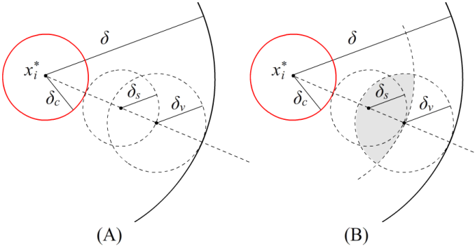
Figure 14: The selection mechanism of SST.

Next, consider the size of the intersection of $\mathcal{B}_{\delta-\delta_{BN}}(x_{i}^{\ast})$ and a ball of radius $\delta_{BN}$ that is entirely enclosed in $\mathcal{B}_{\delta}(x_{i}^{\ast})$. Let $x_{v}$ denote the center of this ball. This intersection, highlighted in Fig. 14(B), represents the area that a sample can be generated so as to return a state from ball $\mathcal{B}_{\delta-\delta_{BN}}(x_{i}^{\ast})$. In the worst case, the center of this ball $\mathcal{B}_{\delta_{BN}}(x_{v})$ could be on the border of $\mathcal{B}_{\delta-\delta_{BN}}(x_{i}^{\ast})$, as seen in Fig. 14 B. Then, the probability of sampling a state in this region can be computed as: $\gamma_{sst}=\inf\mathbb{P}\Big{(}\big{\{}x^{\prime}\text{ returned by {\tt BestNear}}:x^{\prime}\in\mathcal{B}_{\delta}(x_{i}^{\ast})\big{\}}\Big{)}=\frac{\mu(\mathcal{B}_{\delta-\delta_{BN}}(x_{i}^{\ast})\cap\mathcal{B}_{\delta_{BN}}(x_{v}))}{\mu(\mathbb{X}_{f})}$. This is the smallest region that will guarantee selection of a node in $\mathcal{B}_{\delta}(x_{i})$.

$\blacksquare$

Lemma 28 shows that the probability to select a near optimal state within the covering ball sequence with a non-decreasing cost can be lower bounded. It is almost identical to the selection mechanism of RRT-BestNear. Similarly to the analysis of RRT-BestNear, the probability that MonteCarlo-Prop is now again different. The trajectories considered here must enter balls of radius $\delta_{c}$, so the changed probability for MonteCarlo-Prop to generate such a trajectory is $\rho_{\delta\to\delta_{c}}$. With $\gamma_{sst}$ and $\rho_{\delta\to\delta_{c}}$ defined, the completeness of SST can be argued.

Theorem 29.

STABLE Sparse-RRT is probabilistically $\delta$-robustly complete. e.g.,

$$\liminf_{n\to\infty}\mathbb{P}(\ \exists\ \pi\in\Pi^{SST}_{n}:\pi\text{ solution to }(\mathbb{X}_{f},x_{0},\mathbb{X}_{G},\delta))=1.$$

Theorem 30.

STABLE Sparse-RRT is asymptotically $\delta$-robustly near-optimal. e.g.

$$\mathbb{P}\Big{(}\Big{\{}\limsup_{n\to\infty}Y_{n}^{SST}\leq(1+\frac{K_{x}\delta}{C_{\Delta}})\cdot C^{\ast}\Big{\}}\Big{)}=1.$$

The proofs for Theorem 29 and Theorem 30 are almost identical to the proofs of Theorem 24 and Theorem 25 respectively. The only differences are the different probabilities $\gamma_{sst}$ and $\rho_{\delta\to\delta_{c}}$. By changing the radii in the proofs of Theorem 29 and Theorem 30 to their correct values in SST, the proofs hold.

Theorem 31.

In the worst case, the $k^{th}$ segment of the trajectory returned by SST converges linearly to the near optimal one, i.e.,

$$\lim_{n\to\infty}\frac{|\mathbb{P}(E_{k}^{(n+1)})-1|}{|\mathbb{P}(E_{k}^{(n)})-1|}=(1-\gamma\rho_{\delta\to\delta_{c}})\in(0,1).$$

The convergence rate and expected iterations for SST are again almost identical to that of RRT-BestNear, since both the selection mechanism and the propagation probability of SST can be bounded by constants.

The benefit of SST is that the per iteration complexity ends up being smaller than RRT-BestNear. The most expensive operation for the family of algorithms discussed in this paper asymptotically is the near neighbor query. SST delivers noticeable computational improvement over RRT-BestNear due to the reduced size of the tree data structure. The rest of this section examines the influence of the sparse data structure, which is brought by the pruning process in SST.

Among a set of size $n$ points, the average time complexity for a nearest neighbor query is $\mathcal{O}(\log n)$. The average time complexity of the range query for near neighbors is $\mathcal{O}(n)$, since the result is a fixed proportional subset of the whole set. Using this information, it is possible to estimate the overall asymptotic time complexities for RRT-BestNear and SST to return near-optimal solutions with probability at least $1-e^{-1}\approx 63.21\%$.

Lemma 32.

For a $k$ segment optimal trajectory with $\delta$ clearance, the expected running time for RRT-BestNear to return a near-optimal solution with $1-e^{-1}$ probability can be evaluated as: $\mathcal{O}\Big{(}(\frac{k}{\gamma\rho_{\delta\to\delta_{c}}})^{2}\Big{)}$

Proof: Let $N_{p}$ denote $\frac{k}{(1-e^{-1})\gamma\rho}$. The total time computation after $N_{p}$ iterations can be evaluated as, $\mathcal{O}\Big{(}\sum_{i=1}^{N_{p}}c\cdot i\Big{)}=\mathcal{O}\Big{(}c\cdot\frac{N_{p}(N_{p}+1)}{2}\Big{)}=\mathcal{O}\Big{(}(\frac{k}{\gamma\rho_{\delta\to\delta_{c}}})^{2}\Big{)}.$ $\blacksquare$

For RRT-Extend the expected number iterations needed to generate a trajectory can be bounded by $\frac{k}{\rho\gamma_{rrt}}$ (LaValle & Kuffner, 2001a). For the $k^{th}$ segment of a trajectory with $\delta$ clearance, the expected running time for RRT-Extend to return a solution with $1-e^{-1}$ probability can be evaluated as: $\mathcal{O}\Big{(}\frac{k}{\rho\gamma_{rrt}}\cdot\log(\frac{k}{\rho\gamma_{rrt}})\Big{)}$.

Now consider SST. Since each $s\in S$ has claimed a $\delta_{s}$ radius hyper-ball in the state space, then the following is true:

Lemma 33.

For any two distinct witnesses of SST: $s_{1},s_{2}\in S$, where $s_{1}\not=s_{2}$, the distance between them is at least $\delta_{s}$, e.g., $\forall s_{1},s_{2}\in S:||s_{1}-s_{2}||>\delta_{s}$.

Lemma 33 implies that the size of the set $S$ can be bounded, if the free space $\mathbb{X}_{f}$ is bounded.

Corollary 34.

If $\mathbb{X}_{f}$ is bounded, the number of points of the set $S$ and nodes in $\mathbb{V}_{active}$ is always finite, i.e., $\exists M\in\mathcal{O}(\delta^{-d}):|S|=|V_{active}|\leq M$.

Corollary 34 indicates that the total number of points in set $S$ can be bounded. Then, the complexity of any near neighbors query can be bounded. Now the improved time complexity of SST relative to RRT can be formulated.

Lemma 35.

For a $k$ segment optimal trajectory with $\delta$ clearance, the expected running time for SST to return a near-optimal solution with $1-e^{-1}$ probability can be evaluated as, $\mathcal{O}\Big{(}\delta^{-d}\cdot\frac{k}{\gamma\rho_{\delta\to\delta_{c}}}\Big{)}$.

Proof: Let $N_{p}$ denote $\frac{k}{(1-e^{-1})\gamma\rho_{\delta\to\delta_{c}}}$. Due to Corollary 34, the total computation time after $N_{p}$ iterations is: $\mathcal{O}\Big{(}\sum_{i=1}^{N_{p}}c\cdot\delta^{-d}+N_{p}\Big{)}=\mathcal{O}\Big{(}\delta^{-d}\cdot\frac{k}{\gamma\rho_{\delta\to\delta_{c}}}\Big{)}.$ Note that the second term $N_{p}$ describes the worst case of deletion of nodes in $V_{inactive}$ in Algorithm 5. For $N_{p}$ iterations, in the worst case, the algorithm can delete at most $N_{p}$ nodes. $\blacksquare$

5.5 SST* Analysis

In SST, for given $\delta$, $\delta_{s}$, and $\delta_{BN}$ values, $\gamma_{sst}$ and $\rho_{\delta\to\delta_{c}}$ are two constants describing the probability of selecting a near-optimal state for propagation and of successfully propagating to the next ball region. Note that if $\delta_{BN}$ and $\delta_{s}$ are reduced over time, the related $\delta$ value can be smaller. This is the intuition behind why SST^∗ provides asymptotic optimality. If after a sprint of iterations where $\delta_{BN}$ and $\delta_{s}$ are kept static, they are reduced slightly, this should allow for the generation of trajectories with smaller clearance, i.e., closer to the true optimum.

Lemma 36.

For a $\mathcal{B}_{i}$ of radius $\delta$ and a ball $\mathcal{B}_{i}^{\prime}$ with radius $\delta^{\prime}$, such that $\delta^{\prime}/\delta=\alpha$, where $\alpha\in(0,1)$, there is $\frac{\hat{\rho}_{\delta^{\prime}}}{\hat{\rho}_{\delta}}=\alpha^{w+1}$

Lemma 36 says that when the probability $\rho$ decreases over time, it is reduced by a factor $\alpha$ set to the power of the size of the piecewise constant control vector plus one. The proof of this relationship is in Appendix I.

Lemma 37.

Given $\delta>0$, and $\delta_{BN}>0$, for a scale $\alpha\in(0,1)$, let $\delta^{\prime}=\alpha\delta$ and $\delta_{BN}^{\prime}=\alpha\delta_{BN}$, there is $\frac{\gamma^{\prime}}{\gamma}=\alpha^{d}$

Lemma 37 says that a similar relationship exists for values of $\gamma$. This probability is defined purely geometrically in the state space, so its proof is trivial. Now that these relationships have been established, properties of SST^∗ can be shown.

Theorem 38.

$SST^{\ast}$ is probabilistically complete. i.e., $\liminf_{j\to\infty}\mathbb{P}(\{\exists\ x_{goal}\in(V_{n}^{SST^{\ast}}\cap\mathbb{X}_{G})\})=1$

Proof: Let $E_{k,j}^{(i)}$ ($k\geq 1$) denote the event $E_{k}$ (as seen from earlier proofs) at sprint $j$, after $i$ iterations within the sub-function SST. Then:

$$\mathbb{P}(E_{k,j}) =1-\prod_{i=1}^{K(j)}(1-\mathbb{P}(E_{k-1,j}^{(i)})\gamma^{(j)}\rho^{(j)}).$$ (2)

where $\gamma^{(j)}$ and $\rho^{(j)}$ are the values that have been used to bound selection and trajectory generation probability, but for the $\delta_{BN}$ and $\delta_{s}$ values during the $j^{th}$ sprint. Let $c$ be a constant $1\leq c\leq K(j)$ and $p_{c}$ be the value of $\mathbb{P}(E_{k-1,j}^{(c+1)})$ for a given $j$. Note that within the same sprint $j$, Eq. 2 is equivalent to Eq. 28. Let $P_{c}$ be a constant, such that $P_{c}=\prod_{i=1}^{c}(1-\mathbb{P}(E_{k-1,j}^{(i)})\gamma^{(j)}\rho^{(j)})$. Then, Eq. 2 becomes:

$$\mathbb{P}(E_{k,j})=1-P_{c}\prod_{i=c+1}^{K(j)}(1-\mathbb{P}(E_{k-1,j}^{(i)})\gamma^{(j)}\rho^{(j)}).$$ (3)

And clearly, any $\mathbb{P}(E_{k,j}^{(i)})$ ($k\geq 0$) is strictly positive and non-decreasing, as $i$ increases, meaning $p_{c}$ can be used as a lower bound. Then Eq. 3 becomes:

$$\mathbb{P}(E_{k,j}) =1-P_{c}\prod_{i=c+1}^{K(j)}(1-\mathbb{P}(E_{k-1,j}^{(i)})\gamma^{(j)}\rho^{(j)})\geq 1-P_{c}\prod_{i=c+1}^{K(j)}(1-p_{c}\cdot\gamma^{(j)}\rho^{(j)})$$

$$=1-P_{c}(1-p_{c}\cdot\gamma^{(j)}\rho^{(j)})^{K(j)-c}=1-P_{c}\Big{[}(1-p_{c}\cdot\gamma^{(j)}\rho^{(j)})^{\frac{1}{\gamma^{(j)}\rho^{(j)}}}\Big{]}^{\cdot\gamma^{(j)}\rho^{(j)}\cdot(K(j)-c)}.$$ (4)

Since the inequality $(1-\frac{\alpha}{x})^{x}<e^{-\alpha}$ for all $x>1$ and $\alpha>0$. Then Eq. 4 becomes, borrowing from Algorithm 9 the expression for the number of iterations $K(j)$, expression (4) becomes:

$$\mathbb{P}(E_{k,j}) \geq 1-P_{c}\Big{[}(1-p_{c}\cdot\gamma^{(j)}\rho^{(j)})^{\frac{1}{\gamma^{(j)}\rho^{(j)}}}\Big{]}^{\gamma^{(j)}\rho^{(j)}\cdot(K(j)-c)}$$

$$>1-P_{c}(e^{-p_{c}})^{\gamma^{(j)}\rho^{(j)}\cdot(K(j)-c)}$$

$$=1-P_{c}(e^{-p_{c}})^{\gamma^{(j)}\rho^{(j)}\cdot\xi^{-(d+w+1)j}\cdot k_{0}\cdot(1+\log j)-\gamma^{(j)}\rho^{(j)}c}.$$ (5)

Let $\beta=k_{0}\cdot\gamma^{(0)}\rho^{(0)}$, Eq. 5 becomes:

$$\mathbb{P}(E_{k,j}) >1-P_{c}(e^{-p_{c}})^{\gamma^{(j)}\rho^{(j)}\cdot\xi^{-(d+w+1)j}\cdot k_{0}\cdot(1+\log j)-\gamma^{(j)}\rho^{(j)}c}$$

$$=1-P_{c}(e^{-p_{c}})^{\gamma^{(0)}\rho^{(0)}\cdot k_{0}\cdot(1+\log j)-\gamma^{(j)}\rho^{(j)}c}$$

$$=1-P_{c}(e^{-p_{c}})^{\beta\cdot(1+\log j)-\gamma^{(j)}\rho^{(j)}c}$$ (6)

because of Lemma 36-37. As $j$ increases to infinity, the following holds:

$$\lim_{j\to\infty}\mathbb{P}(E_{k,j})>\lim_{j\to\infty}1-P_{c}(e^{-p_{c}})^{\beta\cdot(1+\log j)-\gamma^{(j)}\rho^{(j)}c}=\lim_{j\to\infty}1-\frac{P_{c}\cdot(e^{-p_{c}})^{\beta\cdot(1+\log j)}}{(e^{-p_{c}})^{\gamma^{(j)}\rho^{(j)}c}}=1-\frac{0}{1}=1.$$

Since the limit exists, therefore it is true that $\liminf_{j\to\infty}\mathbb{P}(E_{k,j})=1$. $\blacksquare$

Next, the argument regarding asymptotic optimality.

Theorem 39.

SST^∗ is asymptotically optimal. i.e., $\mathbb{P}(\{\limsup_{j\to\infty}Y_{j}^{SST^{\ast}}=c^{\ast}\})=1$.

Proof: Since event $E_{k,j}$ implies event {$Y_{n}^{SST^{\ast}}\leq(1+c_{\alpha}\delta)\cdot c^{\ast}$}, therefore at the end of the $j^{th}$ sprint, from Eq. 6:

$$\mathbb{P}(\{Y_{j}^{SST}\leq(1+c_{\alpha}\delta^{(j)})\cdot c^{\ast}\})=\mathbb{P}(E_{k,j})>1-\frac{P_{c}\cdot(e^{-p_{c}})^{\beta\cdot(1+\log j)}}{e^{\gamma^{(j)}\rho^{(j)}c}}$$

As $j\to\infty$, clearly $\lim_{j\to\infty}\delta^{(j)}=0$, $\lim_{j\to\infty}\gamma^{(j)}=0$, and $\lim_{j\to\infty}\rho^{(j)}=0$. Then, it is true that:

$$\mathbb{P}(\{\lim_{j\to\infty}Y_{j}^{SST}\leq\lim_{j\to\infty}(1+c_{\alpha}\delta^{(j)})\cdot c^{\ast}\})=\mathbb{P}(\{\lim_{j\to\infty}Y_{j}^{SST}\leq c^{\ast}\})>\lim_{j\to\infty}\Big{[}1-\frac{P_{c}\cdot(e^{-p_{c}})^{\beta\cdot(1+\log j)}}{e^{\gamma^{(j)}\rho^{(j)}c}}\Big{]}=1-\frac{0}{1}=1.$$

$\blacksquare$

Algorithm 9 describes a process that gradually relaxes the ‘‘sparsification’’, which increasingly allows adding active states. At a high level perspective, RRT^∗ employs the same idea implicitly. Recall that RRT^∗ also allows adding states as the algorithm proceeds. The difference is that RRT^∗ adds one state per iteration, while SST^∗ adds a set of states per batch of iterations. Generally speaking, all sampling-based algorithms need to increasingly add states to cover the space. With this approach, sampling-based algorithms avoid knowing the minimum clearance parameter $\delta$.

In SST^∗, the data structure is always a tree, meaning that, at any moment there are $n$ edges and $n+1$ vertices (RRT^∗ trims edges from the underlying RRG graph). The system accessibility property (Ball-Box theorem) guarantees that it is possible to extend edges from one ball region to the next. It is also possible to argue that this will happen almost surely. The Lipschitz continuity assumption of the cost function allows a near-optimal bound on the trajectories. The best-first selection strategy and the pruning process make the above guarantees practical and computationally efficient.

6 Experimental Evaluation

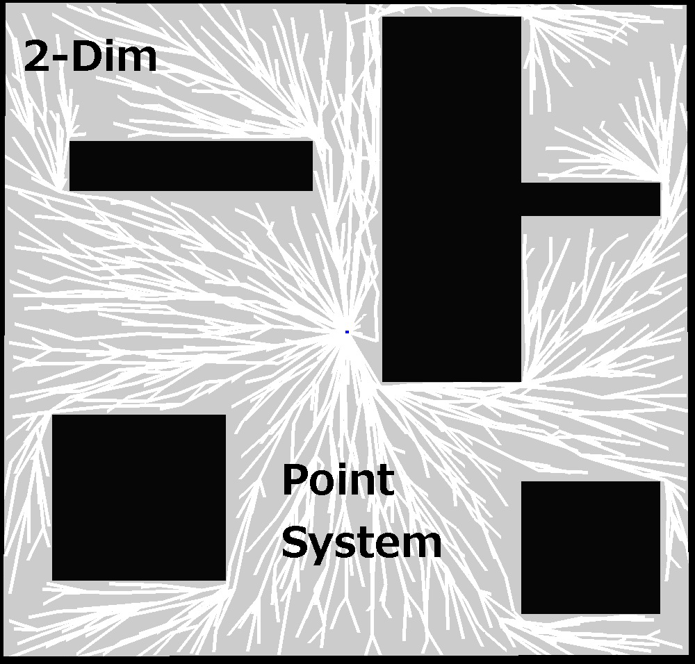
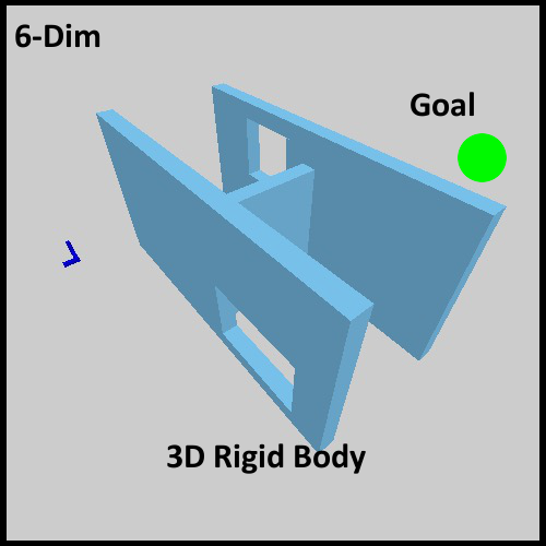
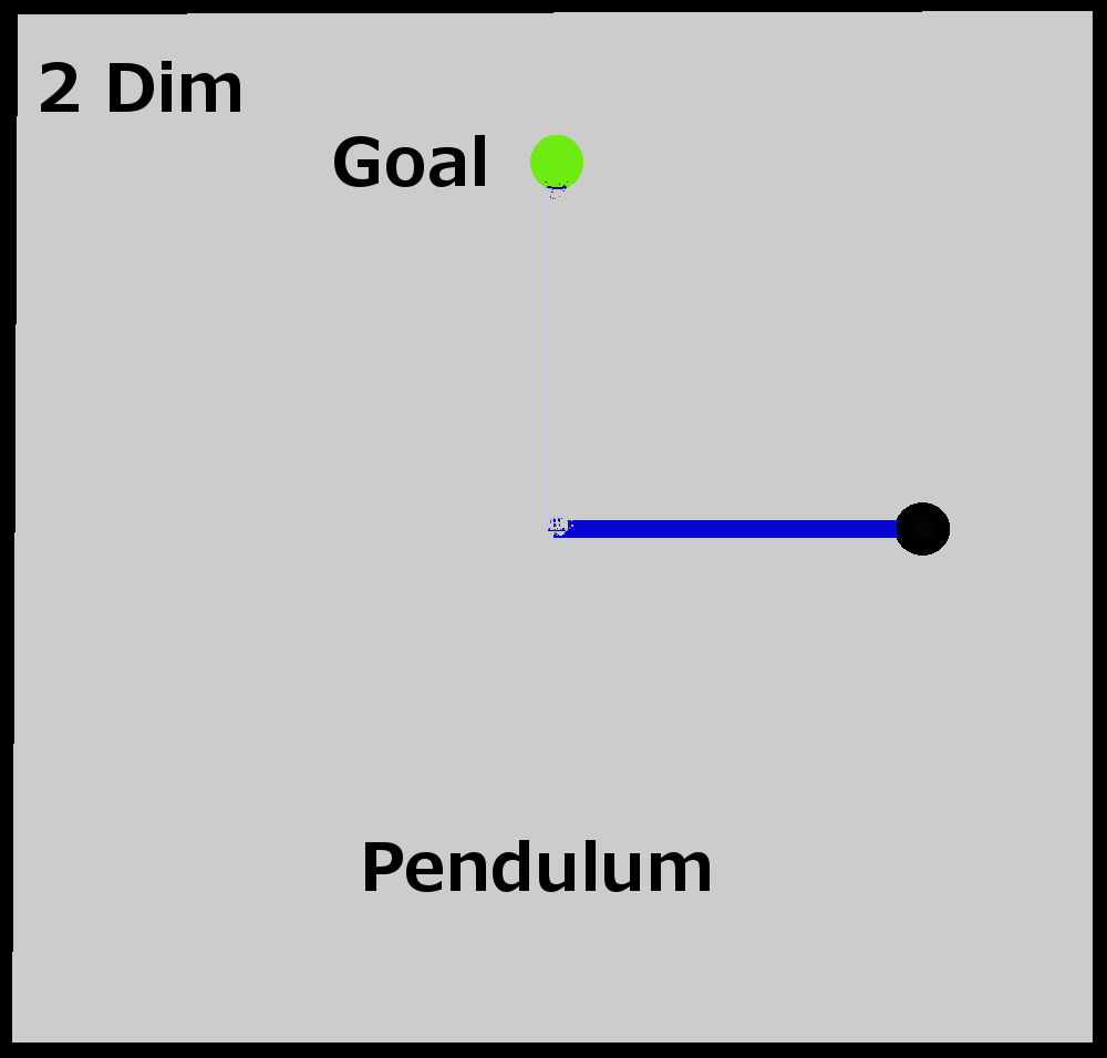
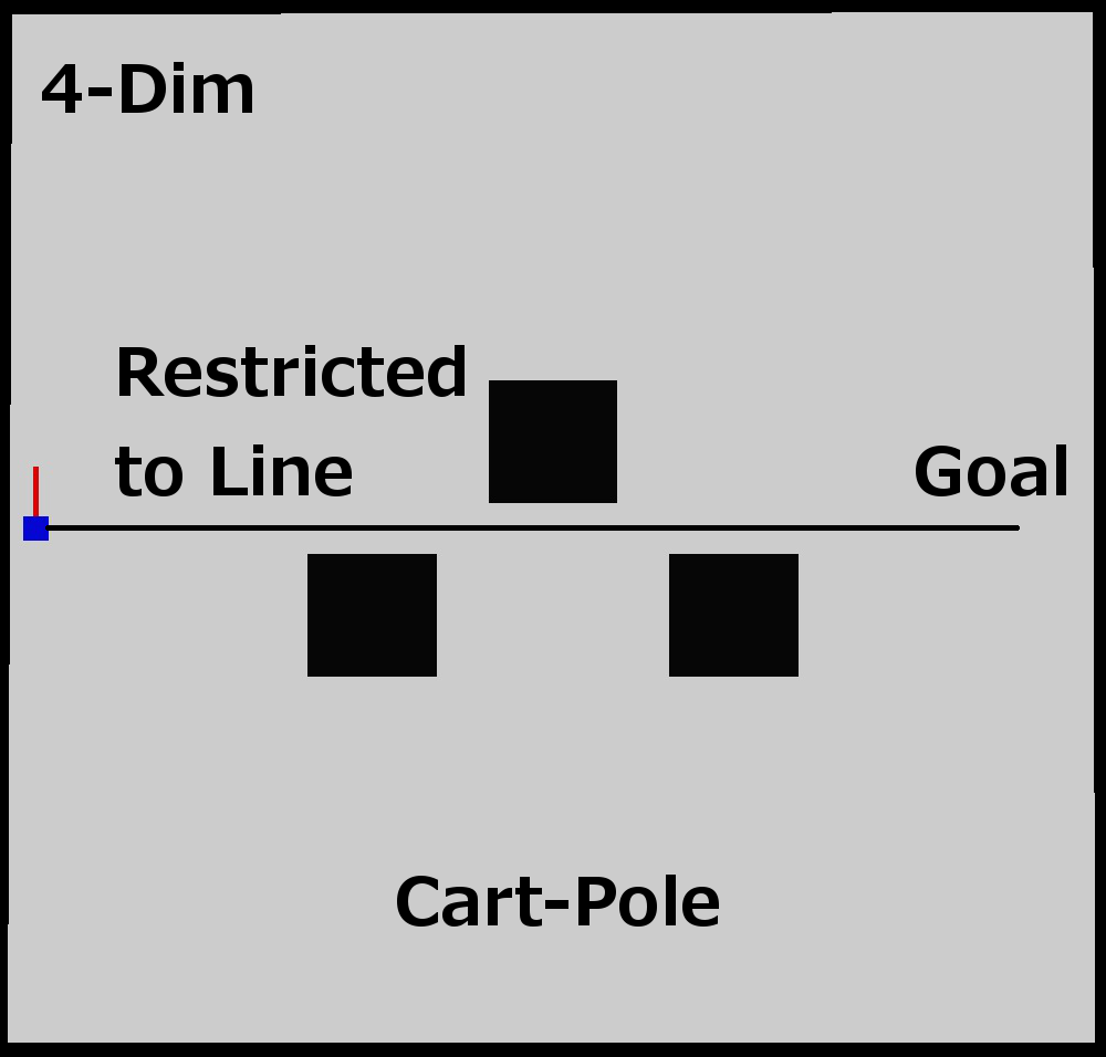
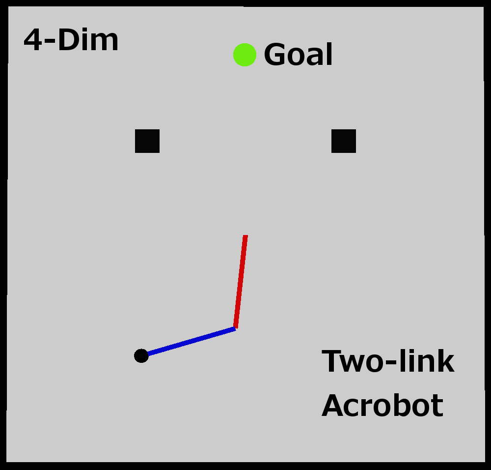
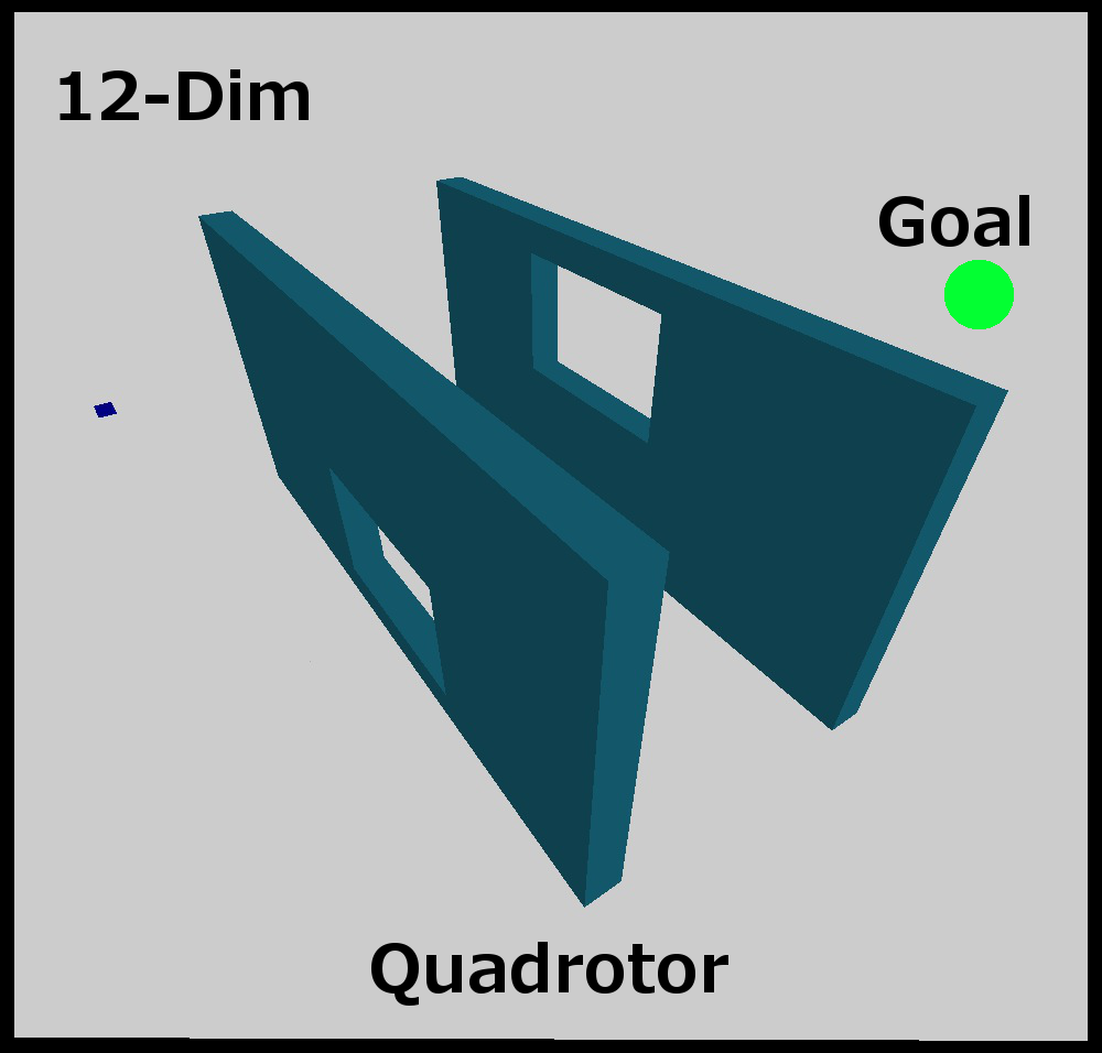
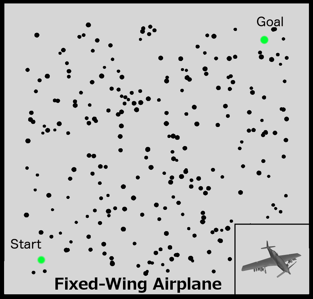
Figure 15: The different benchmarks. From left to right and top to bottom, a kinematic point, 3D rigid body, a pendulum, a cart-pole among obstacles, a passive-active acrobot, a 12-dim quadrotor, fixed-wing aircraft (with much more restricted movement compared to the quadrotor). Each experiment is averaged over 50 runs of each algorithm.

System	Parameters	Distance Function	$\delta_{s}$	$\delta_{BN}$
Kinematic Point	2 Dim. State, 2 Dim. Control	Euclidean Distance	.5	1
3D Rigid Body	6 Dim. State, 6 Dim. Control	Euclidean Distance	2	4
Simple Pendulum	2 Dim. State, 1 Dim. Control, No Damping	Euclidean Distance	.2	.3
Two-Link Acrobot (Spong, 1997)	4 Dim. State, 1 Dim. Control,	Euclidean Distance	.5	1
Cart-Pole (Papadopoulos et al., 2014)	4 Dim. State, 1 Dim. Control,	Euclidean Distance	1	2
Quadrotor (Ai-Omari et al., 2013)	12 Dim. State, 4 Dim. Control,	Distance in ${\mathbb{S}E}3$	3	5
Fixed-Wing Airplane (Paranjape et al., 2013)	9 Dim. State, 3 Dim. Control,	Euclidean Distance in ${\mathbb{R}}^{3}$	2	6

Table 3: The experimental setup used to evaluate SST. Parameters are available in the corresponding references. Values for $\delta_{s}$ and $\delta_{BN}$ have been selected based on the features of each planning challenge.

In order to evaluate the proposed method, a set of experiments involving several different systems have been conducted. The proposed algorithm SST is compared against RRT (LaValle & Kuffner, 2001a) as a baseline and also with another algorithm: (a) if a steering function is available, a comparison with RRT^∗ (Karaman & Frazzoli, 2011) is conducted, (b) if RRT^∗ cannot be used, a comparison with an alternative based on a ‘‘shooting’’ function is utilized (Jeon et al., 2011). Different versions of RRT were evaluated depending on the benchmark. In the case where a steering function is available, RRT corresponds to RRT-Connect. When a steering function is not available, a version of RRT using MonteCarlo-Prop is used, which is similar to RRT-Extend.

The overall results show that SST can provide consistently improving path quality given more iterations as RRT^∗ does for kinematic systems, achieving running times equivalent (if not better than) RRT, and maintaining a small number of nodes, all while using a very simple random propagation primitive.

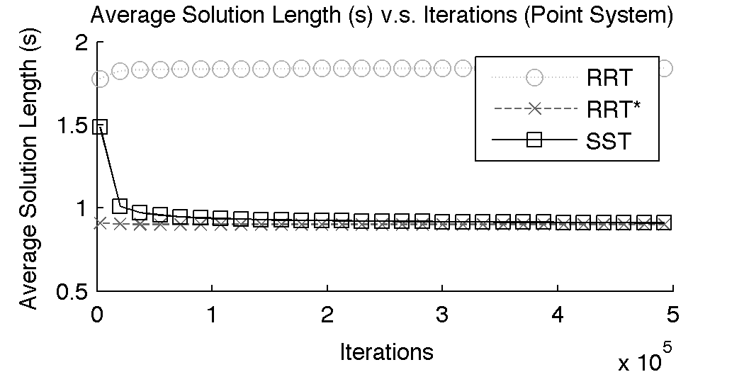
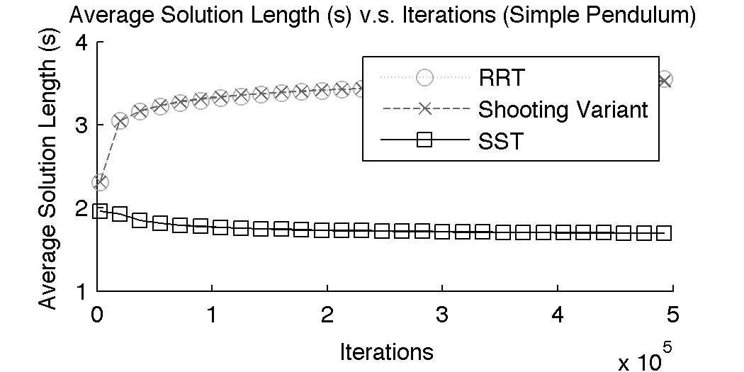
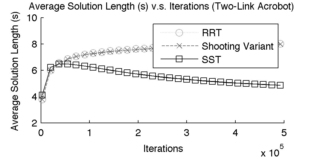
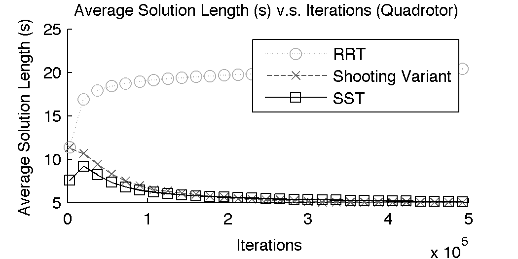
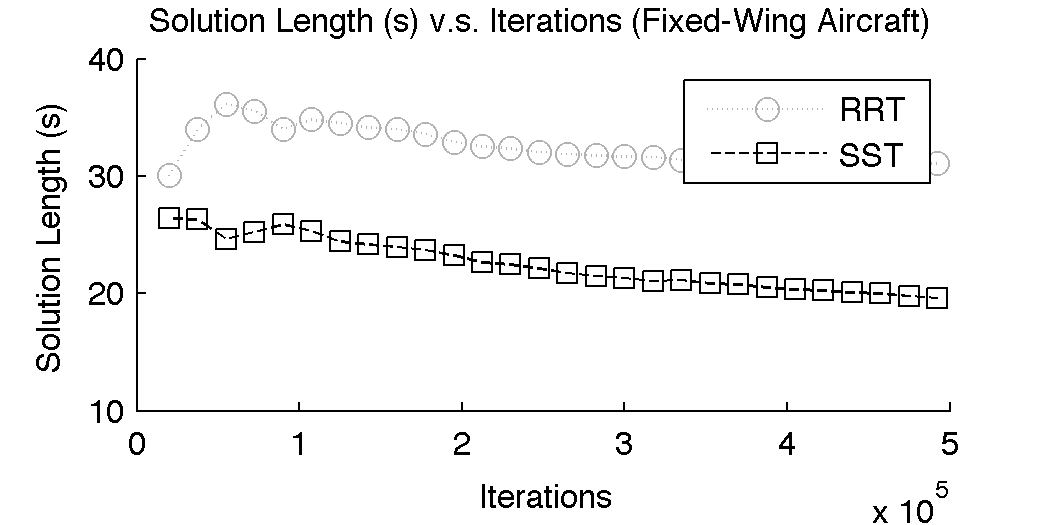
Figure 16: The average cost to each node in the tree for each algorithm (RRT, RRT^∗ or the shooting approach, and SST).

Figure 15 illustrates the various setups that the algorithms have been evaluated on and Table 3 shows details about the experimental setups. The parameters of SST are chosen by hand from an expert user, but could be determined by examining performance of previous attempts.

Kinematic Point. A simple system for a baseline comparison. The state space is 2D $(x,y)$, the control space is 2D $(v,\theta)$, and the dynamics are:

$$\dot{x}=v\cos(\theta)\ \ \ \ \ \dot{y} =v\sin(\theta).$$

3D Rigid Body. A free-flying rigid body. The state space is 6D $(x,y,z,\alpha,\beta,\gamma)$ signifying the space of SE(3) and the control space is 6D $(\dot{x},\dot{y},\dot{z},\dot{\alpha},\dot{\beta},\dot{\gamma})$ representing the velocities of these degrees of freedom.

Simple Pendulum. A pendulum system typical in control literature. The state space is 2D $(\theta,\dot{\theta})$, the control space is 1D $(\tau)$, and the dynamics are:

$$\ddot{\theta}=\frac{(\tau-mgl*\cos(\theta)*0.5)*3}{ml^{2}}.$$

where $m=1$ and $l=1$.

Cart-Pole. Another typical control system where a block mass on a track has to balance a pendulum. The state space is 4D $(x,\theta,\dot{x},\dot{\theta})$ and the control space is 1D $(f)$ which is the force on the block mass. The dynamics are from (Papadopoulos et al., 2014).

Two-link Acrobot. The two-link acrobot model with a passive root joint. The state space is 4D $(\theta_{1},\theta_{2},\dot{\theta_{1}},\dot{\theta_{2}})$ and the control space is 1D $(\tau)$ which is the torque on the active joint. The dynamics are from (Spong, 1997).

Fixed-wing airplane. An airplane flying among cylinders. The state space is 9D $(x,y,z,v,\alpha,\beta,\theta,\omega,\tau)$, the control space is 3D $(\tau_{des},\alpha_{des},\beta_{des})$, and the dynamics are from (Paranjape et al., 2013).

Quadrotor. A quadrotor flying through windows. The state space is 12D $(x,y,z,\alpha,\beta,\gamma,\dot{x},\dot{y},\dot{z},\dot{\alpha},\dot{\beta},\dot{\gamma})$, the control space is 4D $(w_{1},w_{2},w_{3},w_{4})$ corresponding to the rotor torques, and the dynamics are from (Ai-Omari et al., 2013).

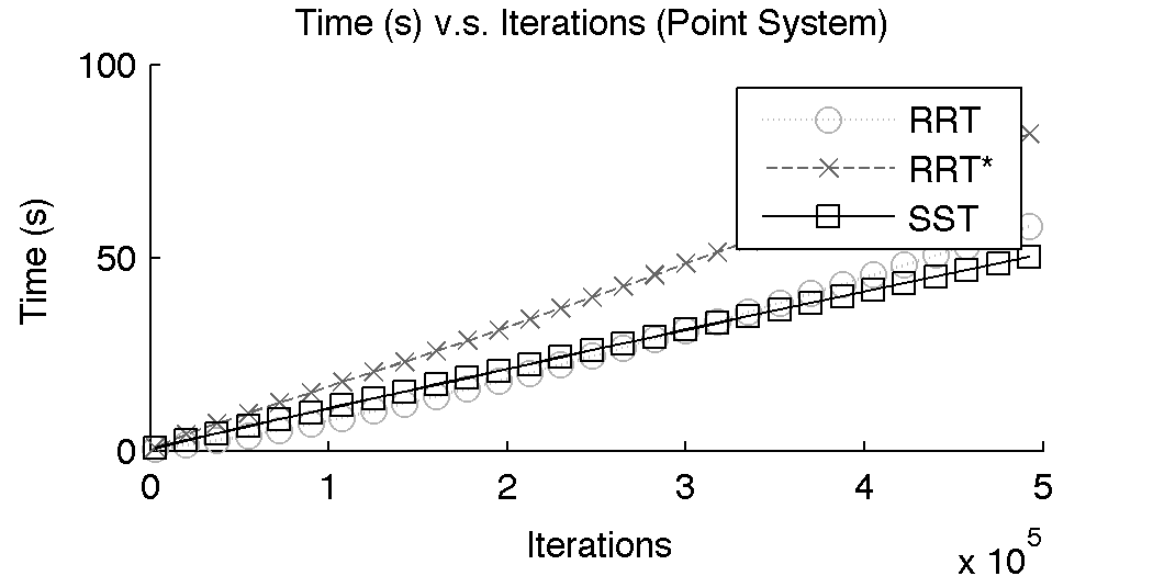
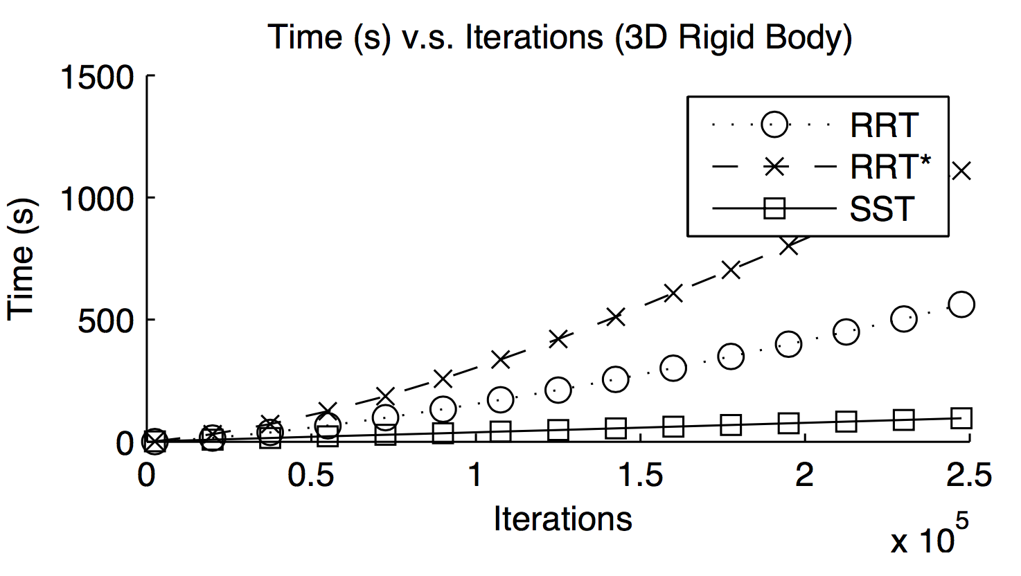
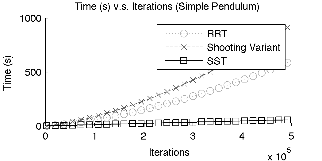
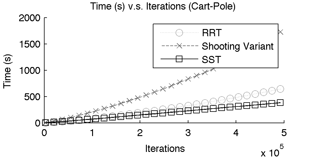
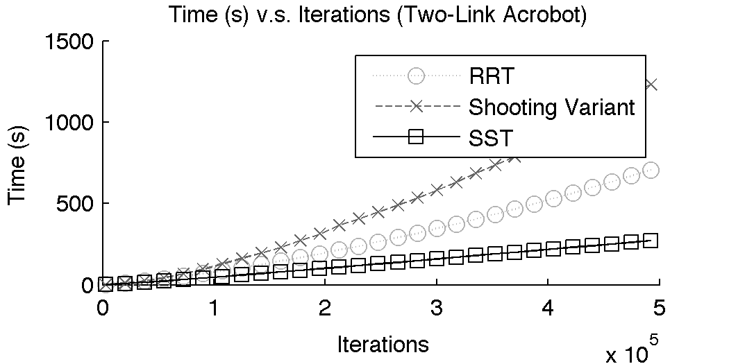
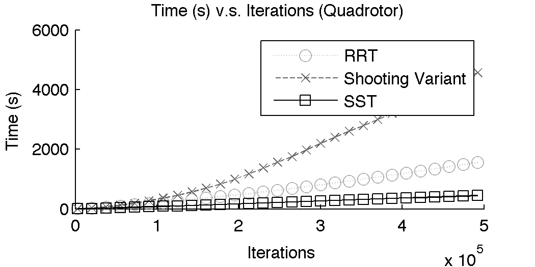
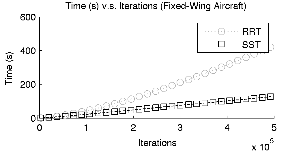
Figure 17: The time for execution for each algorithm (RRT, RRT^∗ or the shooting approach, and SST).

6.1 Quality of Solution Trajectories

In Figure 16 the average solution quality to nodes in each tree is shown. This average is a measure of the quality of trajectories generated to all reachable parts of the state space. In every case, SST is able to improve quality over time. By looking at all of the nodes in the tree as a whole, the global behavior of improving path costs can be observed. RRT will increase this average over time because it chooses suboptimal nodes and further propagates them, thus making those average values increase over time.

It is interesting to note that the approach based on the shooting function had varying success in these scenarios. The systems with highly nonlinear dynamics (e.g., all the systems with a pendulum-like behavior) did not perform better than RRT. This could result from the choice of distance function for these scenarios or from the inaccuracy in the shooting method. Notably, SST does not have this problem for the same distance function and with random propagations and continues to provide good performance. The shooting method did perform well in the quadrotor environment, but failed to return solutions for most of the fixed-wing airplane runs and was therefore omitted.

6.2 Time Efficiency

Figure 17 shows time vs. iterations plots for each of the systems. The graphs show the amount of time it took to achieve a number of iterations. The running time of SST is always comparable or better than RRT. RRT^∗ has a higher time cost per iteration as expected. Initially SST is slightly slower than RRT for the kinematic point, but becomes increasingly more efficient later on. This is explained by Lemma 35, since SST has better running time than RRT given the sparse data structure.

SST has another advantage over other RRT variants. Due to the pruning operation, there is another criterion in addition to being collision-free that newly generated states must satisfy to be added to the tree. Any new state must both be collision-free and dominant in the region around the witness sample in $S$. Because of this, the collision check at Line 8 of Algorithm 5 can be shifted to after Line 15. In the event that collision checking is more expensive than a nearest neighbor query in $S$, this can result in improved computational efficiency depending on the scenario. This strategy was not used in these experiments, but can be beneficial in domains where collision checking is the dominant computational factor.

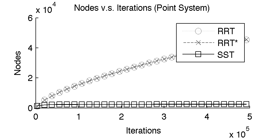
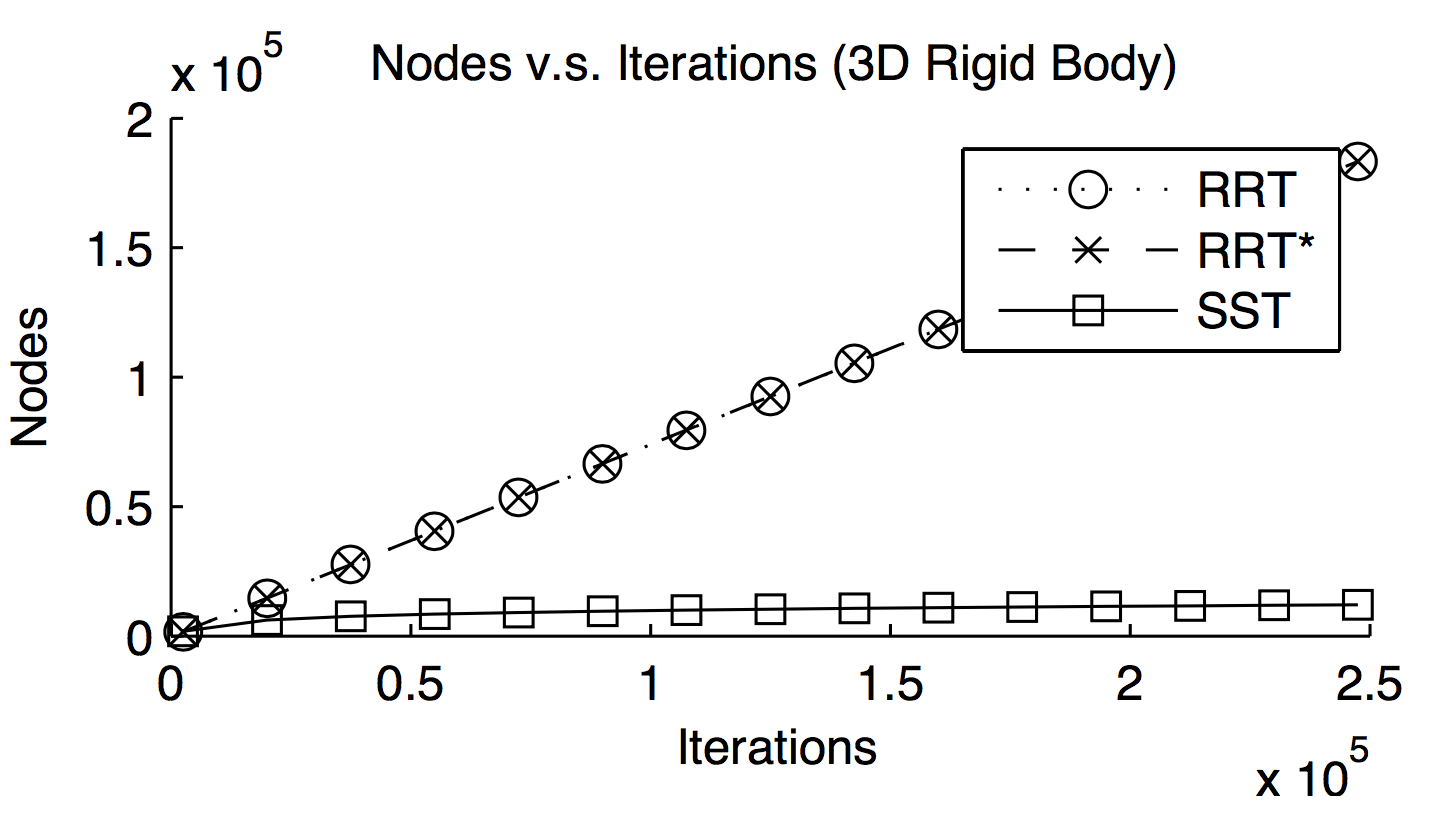
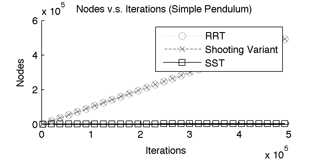
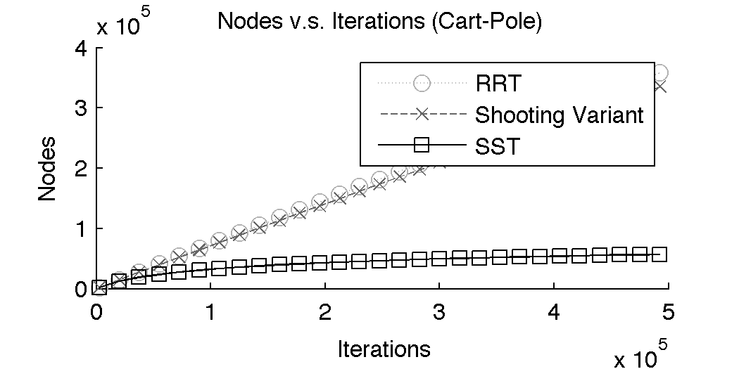
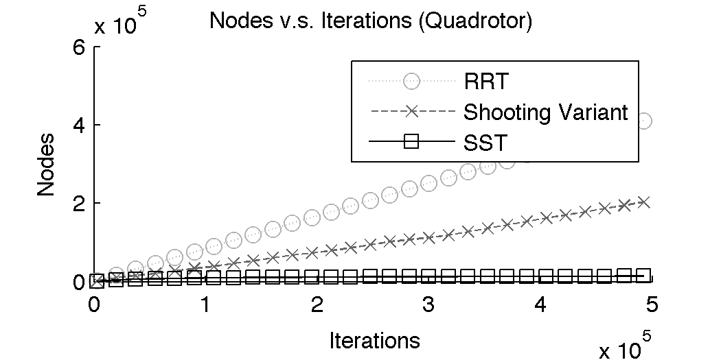
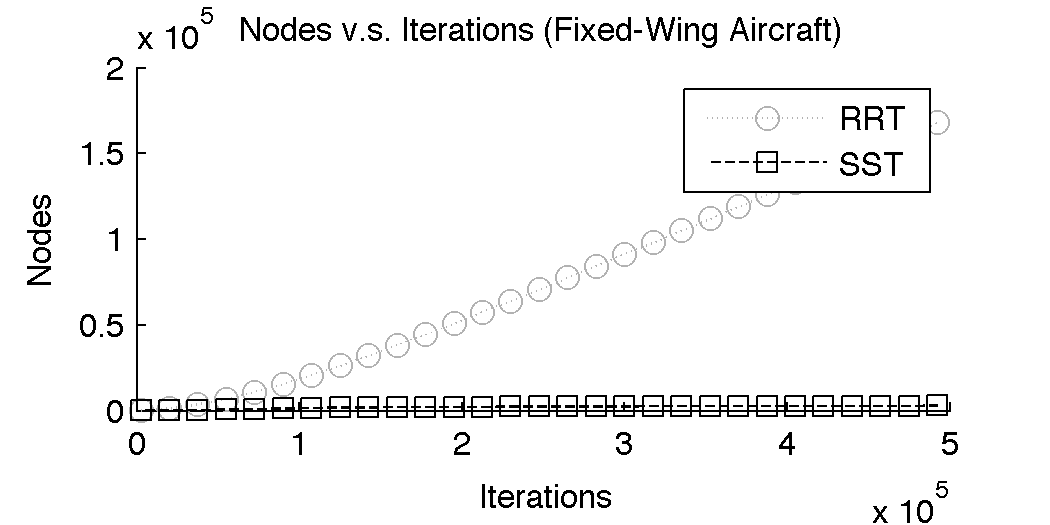
Figure 18: The number of nodes stored in each algorithm (RRT, RRT^∗ or the shooting approach, and SST).

6.3 Space Efficiency

One of the major gains of using SST is the smaller number of nodes that are needed in the data structure. Figure 18 shows the number of nodes stored by each of the algorithms. The number of nodes is significantly lower in SST, even when considering the witness set $S$. The sparse data structure of SST makes the memory requirements quite small, in contrast to RRT and RRT^∗, which do not perform any pruning operations. In the case of shooting, sometimes the inaccuracy of the shooting primitive will cause collisions to occur in resimulated trees, pruning them from the data structure. This can lead to losing solution trajectories.

These results showcase the large efficiency gains when a sparse data structure can be generated. There is a tradeoff, however, between the sparseness of the data structure and allowing for a diverse set of paths to be generated. Path diversity can be helpful for discovering the homotopic class of the optimal solution in practice. In all of these scenarios, there is either only one homotopic class for solutions or the pruning radius $\delta_{s}$ is small enough to allow each homotopic class to be potentially explored. Even considering this, significant pruning can still be achieved.

One can draw parallels between SST and grid-based methods, as both methodologies end up maintaining a discrete set of witness states in the state space. One concern with grid-based approaches is that they have an exponential dependency in the dimensionality of the state space. In the worst case, SST shares the same property. At the same time, however, it has certain advantages. Typically, the discretization followed by grid-based methods corresponds to fixed witnesses defined before the problem is known. In SST the witnesses arise on the fly and are adaptive to the features of the state space. A benefit of following this approach is the capability to find solutions sooner in practice without explicitly constructing or reasoning over the entire grid, which has an exponential number of points. After an initial solution is found, witness nodes can be removed, improving space complexity even further, similar to branch-and-bound techniques.

6.4 Dependence on Parameters

		$\delta_{BN}$
		$1.0$			$1.2$			$1.4$			$1.6$			$1.8$
		IT	IC	FC	IT	IC	FC	IT	IC	FC	IT	IC	FC	IT	IC	FC
$\delta_{s}$	0.2	0.1105	3.4201	1.7782	0.1296	3.2891	1.7798	0.1516	3.2248	1.7866	0.1687	3.0865	1.7890	0.2095	3.0641	1.7949
	0.4	0.1190	3.2445	1.7851	0.0915	3.2614	1.7797	0.0938	3.1364	1.7833	0.0961	3.0506	1.7829	0.0906	3.1027	1.7852
	0.6	0.0603	3.2155	1.7916	0.0999	3.2105	1.7973	0.0670	2.9795	1.7988	0.0671	2.9523	1.7987	0.0679	2.8082	1.7971
	0.8	0.0451	3.0468	1.8229	0.0593	2.9554	1.8273	0.0498	2.8908	1.8193	0.0545	2.8334	1.8232	0.0724	2.6549	1.8416
	1.0	0.0548	2.7695	1.8627	0.0635	2.7371	1.8723	0.0567	2.7365	1.8621	0.0595	2.7185	1.8853	0.0601	2.7493	1.8846

Table 4: A comparison of different parameter choices in SST. The problem setup is the 2D point where the distance function is the typical Euclidean metric. For each parameter selection, the time to compute an initial solution (IT), the initial solution cost in seconds (IC), and final solution cost in seconds (FC) after 60 seconds of execution time.

Table 4 shows statistics for running SST with several different parameter choices. The problem setup is the simple case of the 2D kinematic point. Larger values for the pruning radius, $\delta_{s}$, result in initial solutions being discovered sooner. Larger values also restrict the convergence to better solutions. Larger values for the selection radius, $\delta_{BN}$, provide better solution cost for initial solutions, but requires more computational effort. These tradeoffs can be weighed for the application area depending on the importance of finding solutions early and the quality of those solutions.

6.5 Physically-simulated Car Evaluation

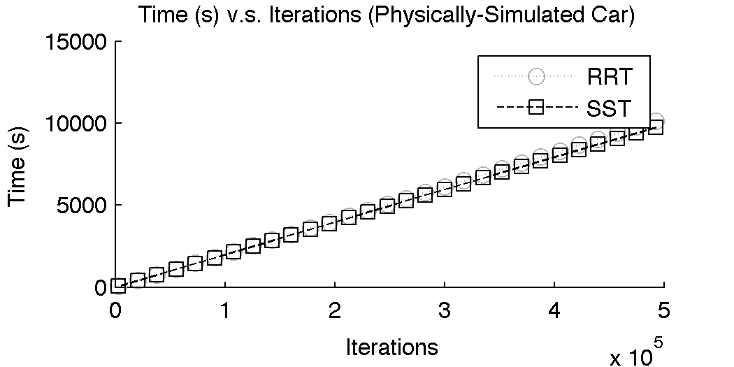
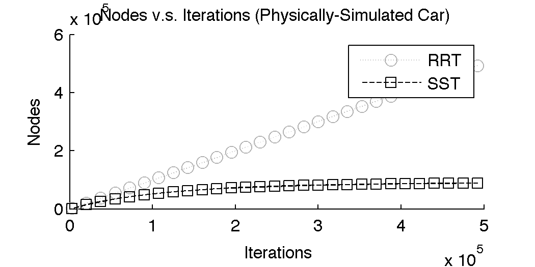
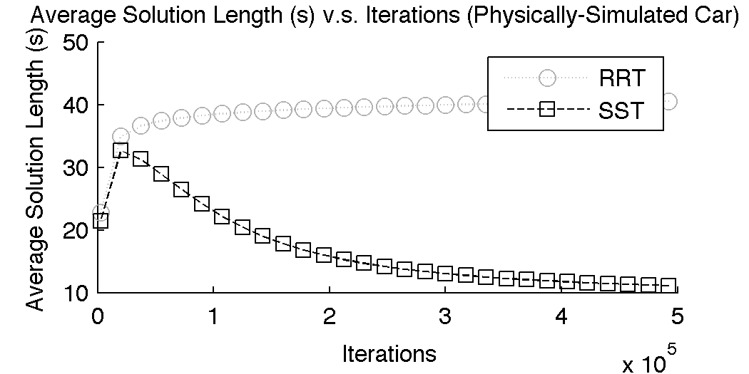
Figure 19: Experimental results for the physically-simulated car-like system. The time complexity of the approach is similar to RRT, but maintains a much smaller data structure.

One of the more interesting applications of SST is in the domain of planning for physically-simulated systems (Coumans, 2012). SST is able to provide improving path quality given enough time and keeps the number of forward propagations to one per iteration as shown in Figure 19. In this setup, the computational cost of propagation overtakes the cost of nearest neighbor queries. Nearest neighbor queries become the bottleneck in problems, such as the kinematic point, where propagation and collision checking are cheap. In the physically simulated case, however, these primitives are expensive, therefore focusing the motion planner on good quality paths is especially important. In this respect, SST is suited to plan for physically-simulated systems.

This physically-simulated car is modeled through the use of a rectangular prism chassis, two wheel axles, and four wheels, creating a system with 7 rigid bodies. These rigid bodies are linked together with virtual joints in the Bullet physics engine (Coumans, 2012). The front axle is permitted to rotate to simulate steering angle and thrust is simulated as a force on the chassis. The data provided in Figure 19 is generated by planning for the car in an open environment and attempting to reach a goal state denoted by x,y and heading.

Using SST for a physically simulated system raises the question of whether this is a case where asymptotic optimality can be argued formally. Note, that in this case, contacts arise between the moving system and the plane. Such contacts typically violate the assumptions specified in the problem setup and in this manner the formal guarantees described in this work do not necessary apply. Nevertheless, it is encouraging that the algorithm is still exhibiting good performance, in terms of being able to improve the quality of the solution computed over time. This is probably because such real-world problems still exhibit a certain level of smoothness that allows the algorithm to prune suboptimal solutions. As described in the Discussion section of this paper, future research efforts will focus on generalizing the provided analysis and include interesting challenges where contacts arise, including dexterous manipulation and locomotion.

6.6 Graph-based Nearest Neighbor Structure

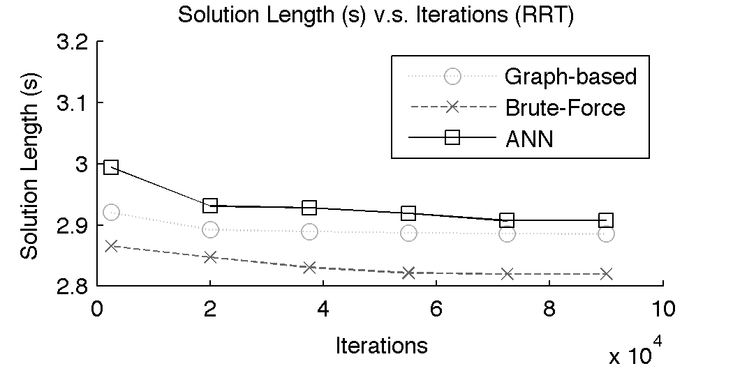
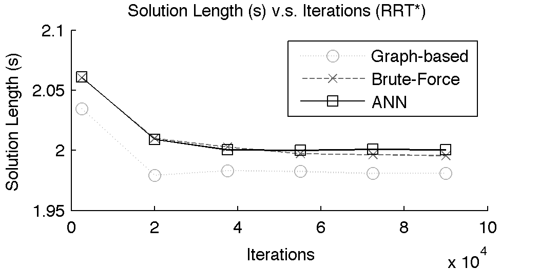
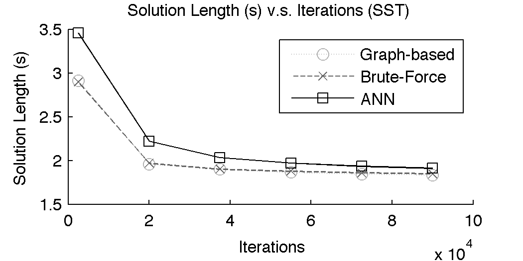
Figure 20: A comparison of three different nearest neighbor structures in terms of solution quality at different iteration milestones for the point system. This is not considering the amount of time to reach these iteration milestones.

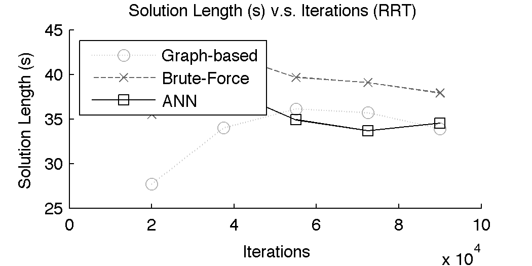
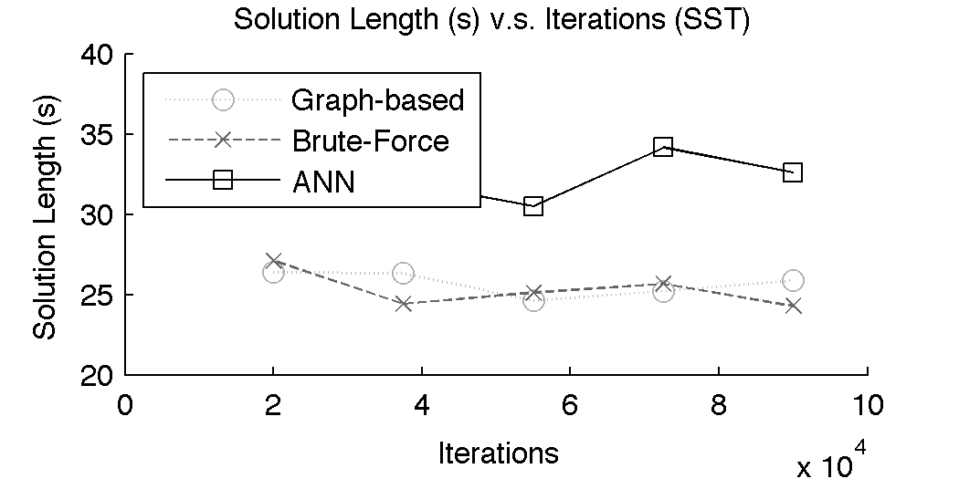
Figure 21: A comparison of three different nearest neighbor structures in terms of solution quality at different iteration milestones for the airplane system. This is not considering the amount of time to reach these iteration milestones.

In order to evaluate the graph-based nearest neighbor structure, comparisons to two other alternatives are shown. First, a baseline comparison with a brute force search is provided. This provides the worst-case performance computationally that more intelligent search methods should be able to overcome. Next, an approximate nearest neighbor structure is used (Arya et al., 1998). This approach follows the popular kd-trees approach to space decomposition and nearest neighbor queries. In the following experiments, the same environments for the kinematic point and the airplane systems are used, and comparisons are made between RRT, RRT^∗, and SST.

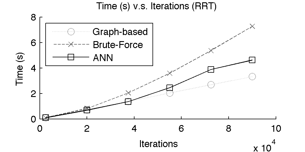
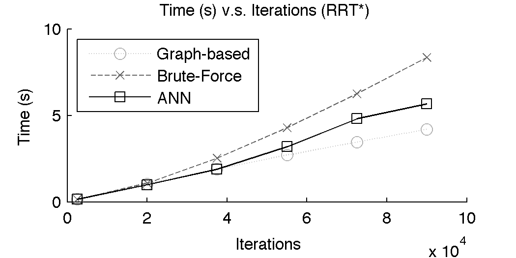
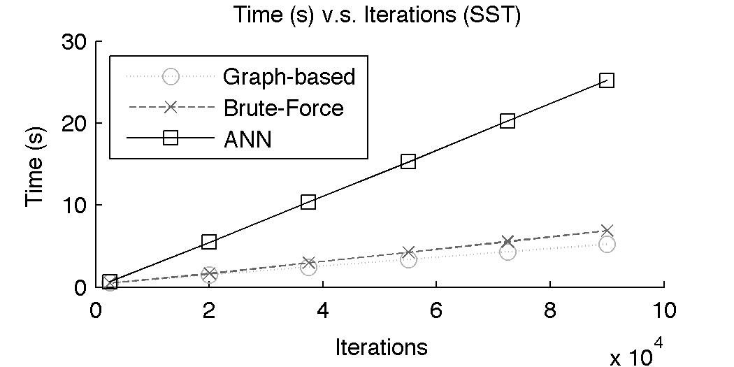
Figure 22: A comparison of three different nearest neighbor structures in terms of time of execution at different iteration milestones for the point system.

A comparison of the resulting solution quality between planners that use different nearest neighbor structures is shown in Figures 20 and 21. In the case of RRT, where the Voronoi bias heavily affects the expansion process, having an exact brute force metric actually provides small benefits in terms of quality. For RRT^∗ and SST, small approximation errors when returning nearest neighbors can actually result in generating longer edges that help in path quality. This causes a small improvement in path quality for these algorithms.

Structure	Single Query	Range Query	$k$-Query
Brute-Force	100%	100%	100%
ANN	100%	93.48%	99.74%
Graph-based	100%	99.96%	100%

Table 5: The accuracy of the graph-based nearest neighbor structure. These results state that over 5000 queries to a data structure holding 50000 states, these are the percentages of queries that were returned with the correct result. Most errors occurred from not returning all relevant results (states that should have been returned) or returning false positives (states that should not have been returned).

In Figure 22, timing data for each of the nearest neighbor structures is shown. As expected in RRT and RRT^∗, the brute force method is worse than either of the approximate structures. The graph-based structure slightly outperforms the alternative method. An interesting effect occurs in the case of SST however. Since SST maintains a small number of nodes for this problem instance, the brute force search can actually be competitive with the graph-based nearest neighbor. The alternative method that does not explicitly handle removal is much slower than the graph structure for SST, mainly due to having to rebuild its internal structure when too many nodes are removed.

Table 5 shows the accuracy of the graph-based method compared to the other methods. While resulting in some query errors, the number of errors is less than the comparison method.

7 Discussion and Conclusion

Recently, the focus in sampling-based motion planning has moved to providing optimality guarantees, while balancing the computational efficiency of the related methods. Achieving this objective for systems with dynamics has generally required the generation of specialized steering functions. This work shows that a fully-random selection/propagation procedure can achieve asymptotic optimality under reasonable assumptions for kinodynamic systems. The same method, however, has a very slow convergence rate to finding high-quality solutions, which indicates that the focus should primarily be on the convergence rate of methods that provide path improvement over time.

To address these issues, this work proposed a new framework for asymptotically optimal sampling-based motion planning. The departure from previous work is the utilization of best-first selection strategy and a pruning process, which allow for fast convergence to high-quality solutions and a sparse data structure. Experiments and analytical results show the running time and space requirements of a concrete implementation of this framework, i.e., the SST approach, are better even than that of the efficient but suboptimal RRT, while SST can still improve path quality over time. This performance increase is seen in many different scenarios, including in the case of a physically-simulated system.

Parameter Selection: The two parameters of SST, namely $\delta_{s}$ and $\delta_{BN}$, directly affect the performance of the algorithm. Since the $\delta_{s}$ radius controls how much pruning SST will perform, it is necessary that this parameter is not set too high because it can lead the algorithm not to discover paths through narrow passages. Practically, $\delta_{s}$ can be as large as the clearance of paths desired from a given problem instance. It is also helpful to choose this value to be smaller than the radius of the goal region, so as to allow the generation of a sample close to the goal.

The parameter $\delta_{BN}$ should be larger than $\delta_{s}$ to allow the tree data structure to properly expand. A value for $\delta_{BN}$ that is too large will result in poor exploration of the state space since nodes closer to the root will be selected repetitively. Overall, a balance between the state space size, $\delta_{BN}$, and $\delta_{s}$ must be maintained to achieve good performance. The SST^∗ approach allows to start the search using rather arbitrary large values for $\delta_{s}$ and $\delta_{BN}$, which then automatically decrease over time.

Finite-time Properties: Since SST maintains a relatively small data structure, and in bounded spaces it results in a finite size data structure, it is interesting to consider the finite-time properties that can be argued (Dobson & Bekris, 2013). This depends significantly on the rate at which the witness set $S$ can cover the free space. After this initial coverage, it may be possible to examine the quality of the existing paths.

Planning under Uncertainty: By removing the requirement of the steering function, SST can be applied to other problems where steering functions are difficult to construct. One of these areas is planning under uncertainty, where planning is performed in belief space. It is difficult to compute a steering function that connects two probability distributions in this domain, but forward propagation can update the corresponding beliefs. Some challenges in applying SST to this domain involve computing appropriate distance metrics for the best first and pruning operations, as well as the increased dimensionality of the problem. Some progress has been recently achieved in this direction, where it has been shown that in the context of the methods described in the current paper a suitable function based on the Earth Mover’s distance can lead to efficient solutions when planning under uncertainty (Littlefield et al., 2015). This can lead eventually to the application of such solutions to important problems that involve significant uncertainty, such as kinodynamic and non-prehensile manipulation (e.g., pushing, throwing, pulling, etc).

Feedback-based Motion Planning: Another extension relates to feedback-based motion planning and the capability to argue that the computed trajectories are dynamically stable. The current work follows the majority of the literature in sampling-based kinodynamic planning and is providing only nominal trajectories and not feedback-based plans or policies. There has been work that takes advantage of sampling in the context of feedback-based motion planning, such as the work on LQR-trees (Tedrake, 2009). Nevertheless, it has been typically difficult to argue about the optimality of a feedback-based solution when it comes to realistic and relatively high-dimensional dynamical robotic systems. In this way, an interesting research direction is to identify the conditions under which it will be possible to provide such guarantees in the context of feedback-based planning.

Real-world Experiments and Applications: It is also important to evaluate the effectiveness of the approach on real systems with significant dynamics, especially aerial systems that perform aggressive maneuvers and systems modeled through the use of physics engines. For example, future planetary exploration missions may involve more capable rovers. They will have the capability to move at higher speeds in low gravity environments, potentially acquiring ballistic trajectories for small periods of time. Thus, reasoning about the dynamics becomes more important during the planning process. SST may be useful in this domain to optimize paths with respect to path length, energy expenditure, or the sensitivity of the sensor payload on-board.

Locomotion and Dexterous Manipulation: Other potential research domains where SST may be used include locomotion and dexterous manipulation. These challenges involve planning using models of contact between objects and physical considerations, such as balancing of a locomotion system or stability of a grasp for a manipulator. The use of a physics engine to model friction and mass effects can be useful here. As demonstrated above, SST provides control sequences that improve over time when a physics engine is used. Nevertheless, the presence of contacts introduces important complexities that are not currently handled by the presented analysis.

In particular, there are two critical assumptions which complicate the generalization of the provided results: (a) the system dynamics are expressed in the form of equation 1, which is a nonlinear ordinary differential equation, and (b) the manifolds in which the systems live are smooth subsets of a $d$-dimensional Euclidean space. These assumptions do not allow to consider models of rigid body dynamics and stick-slip friction, which are useful idealizations of locomotion and dexterous manipulation. Such systems exhibit jump-discontinuities and in general cannot be represented by expressions of the form in Equation 1. There is also a question of whether it is possible to address challenges in spaces, which are not locally Euclidean.

It would be interesting to study manifolds generated by contact constraints. Such manifolds can be algebraic varieties, which need not be smooth. Furthermore, such manifolds can be of different dimensions, as finger gaiting and locomotion problems really don’t live on varieties of a single dimension, but live on stratified sets in a higher-dimensional ambient state space. These issues motivate further research in the direction of providing general sampling-based algorithms that exhibit asymptotic optimality guarantees for proper models of dexterous manipulation and locomotion systems.

Appendix A

This appendix provides an informal proof of Lemma 6, which argues that given Assumption 5, there exist $\delta$-similar trajectories for any specific trajectory $\pi$. The existence of $\delta$-similar trajectories relates to notions that have been used in previous analysis efforts, such as the linking sequence in $\epsilon$-good free spaces (Hsu et al. 2002), or attraction sequences (LaValle & Kuffner 2001a), or being homotopic in $\delta$-interior of $X_{free}$ (Karaman & Frazzoli 2011, 2013).

Lemma 6. Let there be a trajectory $\pi$ for a system satisfying Eq. 1 and Chow’s condition. Then there exists a positive value $\delta_{0}$ called the dynamic clearance, such that: $\forall\ \delta\in(0,\delta_{0}]$, $\forall\ x_{0}^{\prime}\in\mathcal{B}_{\delta}(\pi(0))$, and $\forall\ x_{1}^{\prime}\in\mathcal{B}_{\delta}(\pi(t_{\pi}))$, there exists a trajectory $\pi^{\prime}$, so that: (i) $\pi^{\prime}(0)=x_{0}^{\prime}$ and $\pi^{\prime}(t_{\pi^{\prime}})=x_{1}^{\prime}$; (ii) $\pi$ and $\pi^{\prime}$ are $\delta$-similar trajectories.

Proof Sketch: Informally speaking, Chow’s condition implies that the Ball Box theorem holds. It also implies that the manifold $\mathbb{X}_{f}$ is regular and involutory (Choset et al. 2005). A real-analytic control-affine system is small-time locally accessible (STLA), if and only if the distribution satisfies Chow’s condition (Sussmann 1987). Assume every state on the optimal trajectory is a regular point. Then, the sub-Riemannian ball up to a small constant radius $t_{\epsilon}$ contains a weighted box of the same dimension of the state space and it is oriented according to vector fields of the Lie brackets. The bases are real analytical. Therefore there exists an open neighborhood at each point $x$ such that the bases evaluated at a different point $x^{\prime}$ converge to the bases at $x$ as $x^{\prime}$ approaches $x$. Then, the weighted boxes centered by two sufficiently close states have a non-empty intersection. It implies that a hyper ball of some positive radius $\delta_{0}$ can be fitted into this intersection region. Overall, there are two sufficiently close hyper-ball regions on the optimal trajectory such that between any point $x$ in one ball and any point in the other ball there exists a horizontal curve and the length of the curve is less or equal to the radius $t_{\epsilon}$ of the sub-Riemannian ball. Then concatenating all hyper balls along a specified trajectory, results in the generation of $\delta$-similar trajectories. $\blacksquare$

Appendix B

This appendix proves Theorem 15, which shows that sampling piece-wise constant controls can generate trajectories that are $\delta$-similar to one another. If one trajectory in question is an optimal one, then a trajectory that is $\delta$-similar to that optimal trajectory can be generated.

Theorem 15. For two trajectories $\pi$ and $\pi^{\prime}$ such that $\pi(0)=\pi^{\prime}(0)=x_{0}$ and $\Delta u=\sup_{t}(||u(t)-u^{\prime}(t)||)$:

$$||\pi^{\prime}(T)-\pi(T)||<K_{u}\cdot T\cdot e^{K_{x}\cdot T}\cdot\Delta u,$$

for any period $T\geq 0$.

Proof: Given Assumption 5, for any two states $x_{0},x_{1}$ and two controls $u_{0},u_{1}$:

$$||f(x_{0},u_{0})-f(x_{0},u_{1})||\leq K_{u}||u_{0}-u_{1}||\ \ \ \ \ ||f(x_{0},u_{1})-f(x_{1},u_{1})||\leq K_{x}||x_{0}-x_{1}||.$$

By summing these two inequalities:

$$||f(x_{0},u_{0})-f(x_{0},u_{1})||+||f(x_{0},u_{1})-f(x_{1},u_{1})||\leq K_{u}||u_{0}-u_{1}||+K_{x}||x_{0}-x_{1}||.$$ (7)

Given the Euclidean distance, the following inequality is true:

$$||f(x_{0}u_{0})-f(x_{1},u_{1})||\leq||f(x_{0},u_{0})-f(x_{0},u_{1})||+||f(x_{0},u_{1})-f(x_{1},u_{1})||.$$

By joining this with (7):

$$||f(x_{0},u_{0})-f(x_{1},u_{1})||\leq K_{u}||u_{0}-u_{1}||+K_{x}||x_{0}-x_{1}||.$$ (8)

Now, divide $[0,T]$ into $n$ segments with equal length $\Delta t$. Approximating the value of a trajectory $\pi(T)$ using Euler’s Method, there is a sequence of states $\{x_{0},x_{1},...,x_{n}\}$. Let $u_{i}$ denote $u(i\Delta t)$ corresponding to the control applied at each state.

$$x_{i}=f(x_{i-1},u_{i-1})\Delta t+x_{(i-1)}.$$

For two trajectories $\pi$ and $\pi^{\prime}$ such that $\pi(0)=\pi^{\prime}(0)=x_{0}$, $u(t)$ and $u^{\prime}(t)$ are the corresponding control functions. Then:

$$x_{n}=x_{n-1}+f(x_{n-1},u_{n-1})\Delta t$$

$$x_{n}^{\prime}=x_{n-1}^{\prime}+f(x_{n-1}^{\prime},u_{n-1}^{\prime})\Delta t.$$

Then:

$$|x_{n}-x_{n}^{\prime}||\leq||x_{n-1}-x_{n-1}^{\prime}||+||f(x_{n-1},u_{n-1})-f(x_{n-1}^{\prime},u_{n-1}^{\prime})||\Delta t.$$ (9)

Using (8) and (9):

$$||x_{n}-x_{n}^{\prime}||\leq||x_{n-1}-x_{n-1}^{\prime}||+(K_{u}||u_{n-1}-u_{n-1}^{\prime}||+K_{x}||x_{n-1}-x_{n-1}^{\prime}||)\Delta t,$$

$$||x_{n}-x_{n}^{\prime}||\leq K_{u}\Delta t||u_{n-1}-u_{n-1}^{\prime}||+(1+K_{x}\Delta t)||x_{n-1}s-x_{n-1}^{\prime}||.$$ (10)

Reusing (10) to expand $||x_{n-1}-x_{n-1}^{\prime}||$:

$$||x_{n}-x_{n}^{\prime}||\leq K_{u}\Delta t||u_{n-1}-u_{n-1}^{\prime}||+(1+K_{x}\Delta t)(K_{u}\Delta t||u_{n-2}-u_{n-2}^{\prime}||+(1+K_{x}\Delta t)||x_{n-2}-x_{n-2}^{\prime}||).$$

$$||x_{n}-x_{n}^{\prime}||\leq K_{u}\Delta t||u_{n-1}-u_{n-1}^{\prime}||+(1+K_{x}\Delta t)K_{u}\Delta t||u_{n-2}-u_{n-2}^{\prime}||+(1+K_{x}\Delta t)^{2}||x_{n-2}-x_{n-2}^{\prime}||).$$

By repeatedly expanding the right side:

$$||x_{n}-x_{n}^{\prime}||\leq(1+K_{x}\Delta t)^{n}||x_{0}-x_{0}^{\prime}||+K_{u}\Delta t||u_{n-1}-u_{n-1}^{\prime}||+(1+K_{x}\Delta t)K_{u}\Delta t||u_{n-2}-u_{n-2}^{\prime}||+$$

$$\cdots+(1+K_{x}\Delta t)^{n-1}K_{u}\Delta t||u_{0}-u_{0}^{\prime}||.$$

Since $x_{0}=x_{0}^{\prime}=x_{0}$, and $\Delta u=max_{i=0}^{n-1}(||u_{i}-u_{i}^{\prime}||$.:

$$||x_{n}-x_{n}^{\prime}||\leq K_{u}\Delta t\sum\limits_{i=0}^{n-1}(1+K_{x}\Delta t)^{i}\Delta u.$$

Since $n\Delta t=T$:

$$||x_{n}-x_{n}^{\prime}||\leq K_{u}T\frac{1}{n}\sum\limits_{i=0}^{n-1}(1+\frac{K_{x}T}{n})^{i}\Delta u$$

Due to the fact that $1<(1+\frac{\alpha}{n})^{i}<e^{\alpha}$, where $1\leq i\leq n$ and $\alpha>0$:

$$||x_{n}-x_{n}^{\prime}||<K_{u}Tn\frac{1}{n}e^{K_{x}T}\Delta u\Rightarrow||x_{n}-x_{n}^{\prime}||<K_{u}Te^{K_{x}T}\Delta u.$$

Given Assumption 5, Euler’s method converges to the solution of the Initial Value Problem. Then:

$$||\pi(T)-\pi^{\prime}(T)||=\lim_{n\to\infty}||x_{n}-x_{n}^{\prime}||\text{, where }n\Delta t=T.$$

Therefore:$||\pi(T)-\pi^{\prime}(T)||<K_{u}Te^{K_{x}T}\Delta u$ $\blacksquare$

Appendix C

This appendix proves Theorem 18. The proof shows that given an optimal trajectory, it is possible for NAIVE_RANDOM_TREE to generate a trajectory that is close to the optimal. In effect, this shows that NAIVE_RANDOM_TREE is probabilistically complete. Appendix D will examine the path cost of this generated trajectory.

Theorem 18. NAIVE_RANDOM_TREE will eventually generate a $\delta$-similar trajectory to any optimal trajectory for any robust clearance $\delta>0$.

Proof: Let $\pi^{\ast}$ denote an optimal trajectory of cost $C^{\ast}$ for a $\delta$-robustly feasible motion planning problem ($\mathbb{X}_{f}$, $x_{0}$, $\mathbb{X}_{G}$, $\delta$) and consider the covering ball sequence $\mathbb{B}$($\pi^{\ast}(t)$, $\delta$, $C_{\Delta}$) over the optimal trajectory. Recall that from Def. 14 and Assumption 11, for a given value $T_{prop}$, which is one parameter of MonteCarlo-Prop, it is always possible to find a value $C_{\Delta}$ such that a ball sequence can be defined. Consider the event $\neg E_{k}^{(n)}$ that the algorithm fails to generate any near-optimal trajectory inside a $\delta$-ball centered at the $k^{th}$ segment of $\pi^{\ast}$, $\mathcal{B}_{\delta}(x_{k}^{\ast})$, after $n$ iterations, which only happens when all the $n$ consecutive iterations fail, i.e.:

$$\neg E_{k}^{(n)} =\neg A_{k}^{(1)}\cap\neg A_{k}^{(2)}\cap\text{ ... }\cap\neg A_{k}^{(n)}$$

$$\mathbb{P}(\neg E_{k}^{(n)}) =\mathbb{P}(\neg A_{k}^{(1)})\cdot\mathbb{P}(\neg A_{k}^{(2)}|\neg A_{k}^{(1)})\cdot\text{...}\cdot\mathbb{P}(\neg A_{k}^{(n)}|\bigcap_{j=1}^{n-1}\neg A_{k}^{(j)}).$$ (11)

The probability that $\neg A_{k}^{(n)}$ happens given $\bigcap_{j=1}^{n-1}\neg A_{k}^{(j)}$ is equivalent to the probability of failing to generate a trajectory to $\mathcal{B}_{\delta}(x_{k-1}^{\ast})$ plus the probability that a trajectory has been generated to $\mathcal{B}_{\delta}(x_{k-1}^{\ast})$, but the algorithm has to generate a new trajectory to $\mathcal{B}_{\delta}(x_{k}^{\ast})$, i.e.:

$$\mathbb{P}(\neg A_{k}^{(n)}|\bigcap_{j=1}^{n-1}\neg A_{k}^{(j)}) =\mathbb{P}(\neg E_{k-1}^{(n)})+\mathbb{P}(E_{k-1}^{(n)})\cdot\mathbb{P}(\{\text{fail stepping to }\mathcal{B}_{\delta}(x_{k}^{\ast})\})$$

$$\leq\mathbb{P}(\neg E_{k-1}^{(n)})+\mathbb{P}(E_{k-1}^{(n)})(1-\frac{\rho_{\delta\to\delta}}{n})$$

$$=1-\mathbb{P}(E_{k-1}^{(n)})\cdot\frac{\rho_{\delta\to\delta}}{n}.$$ (12)

Therefore, using Equation 11 and Equation 12:

$$\mathbb{P}(E_{k}^{(n)}) \geq 1-\prod_{j=1}^{n}(1-\mathbb{P}(E_{k-1}^{(j)})\cdot\frac{\rho_{\delta\to\delta}}{j}).$$ (13)

For the base case, $\mathbb{P}(E_{0}^{(j)})=1$ because $x_{0}$ is always in $\mathcal{B}_{\delta}(x_{0})$. Then, consider event $E_{1}$ from iteration 1 to $n$ using Equation (13), and set $y^{(n)}_{1}=\prod_{j=1}^{n}(1-\frac{\rho_{\delta\to\delta}}{j})$:

$$\mathbb{P}(E_{1}^{(n)})\geq 1-\prod_{j=1}^{n}(1-\frac{\rho_{\delta\to\delta}}{j})=1-y^{(n)}_{1}.$$

The logarithm of $y^{(n)}_{1}$ behaves as follows:

$$\log y^{(n)}_{1}=\log\prod_{j=1}^{n}(1-\frac{\rho_{\delta\to\delta}}{j})=\sum_{j=1}^{n}\log(1-\frac{\rho_{\delta\to\delta}}{j})<\sum_{j=1}^{n}-\frac{\rho_{\delta\to\delta}}{j}=-\rho_{\delta\to\delta}\cdot\sum_{j=1}^{n}\frac{1}{j}.$$ (14)

Clearly, Equation 14 diverges as $n\to\infty$:

$$\lim_{n\to\infty}\log y^{(n)}_{1} <\lim_{n\to\infty}-\rho_{\delta\to\delta}\cdot\sum_{j=1}^{n}\frac{1}{j}=-\infty\iff\lim_{n\to\infty}y^{(n)}_{1}=0.$$

$$\lim_{n\to\infty}\mathbb{P}(E_{1}^{(n)})\geq=1-0=1.$$ (15)

Now consider the induction step, if $\lim_{n\to\infty}\mathbb{P}(E_{k-1}^{(n)})=1$, we need to show that the same will be true for $E_{k}^{(n)}$. Similarly, set $y_{k}^{(n)}=\prod_{j=1}^{n}(1-\mathbb{P}(E_{k-1}^{(j)})\cdot\frac{\rho_{\delta\to\delta}}{j})$. The logarithm of $y_{k}^{(n)}$ behaves as follows:

$$\log y_{k}^{(n)}=\log\prod_{j=1}^{n}(1-\mathbb{P}(E_{k-1}^{(j)})\cdot\frac{\rho_{\delta\to\delta}}{j})=\sum_{j=1}^{n}\log(1-\mathbb{P}(E_{k-1}^{(j)})\cdot\frac{\rho_{\delta\to\delta}}{j})<-\rho_{\delta\to\delta}\cdot\sum_{j=1}^{n}\frac{\mathbb{P}(E_{k-1}^{(j)})}{j}.\vspace{-0.05in}$$ (16)

Next, we want to show that for any constant $c_{1}\in(0,1)$:

$$\sum_{j=1}^{\infty}\frac{\mathbb{P}(E^{(j)}_{k-1})}{j}>\sum_{j=1}^{\infty}\frac{c_{1}}{j}.$$

To show the above expression holds, let $c_{2}$ be another constant such that $c_{1}<c_{2}<1$. Clearly, Equation 13 indicates that $E^{(n)}_{k}$ monotonically increases when $\rho_{\delta\to\delta}>0$ and $\mathbb{P}(E^{(j)}_{k-1})>0$. From the induction assumption, $\lim_{n\to\infty}\mathbb{P}(E_{k-1}^{(n)})=1$, then there exist corresponding numbers $j_{1}<j_{2}$ such that $c_{1}\geq\mathbb{P}(E_{k-1}^{(j_{1}-1)}),c_{1}<\mathbb{P}(E_{k-1}^{(j_{1})})$ and $c_{2}\geq\mathbb{P}(E_{k-1}^{(j_{2}-1)}),c_{2}<\mathbb{P}(E_{k-1}^{(j_{2})})$.

Now examine the following summation from $j_{1}$ to $\infty$, according to the definition of summation:

$$\sum_{j=j_{1}}^{\infty}\frac{\mathbb{P}(E^{(j)}_{k-1})-c_{1}}{j}$$ (17)

$$= \sum_{j=j_{1}}^{j_{2}-1}\frac{\mathbb{P}(E^{(j)}_{k-1})-c_{1}}{j}+\sum_{j=j_{2}}^{\infty}\frac{\mathbb{P}(E^{(j)}_{k-1})-c_{1}}{j}$$

$$> \sum_{j=j_{1}}^{j_{2}-1}\frac{\mathbb{P}(E^{(j)}_{k-1})-c_{1}}{j}+\sum_{j=j_{2}}^{\infty}\frac{c_{2}-c_{1}}{j}=\infty.$$ (18)

Clearly, the first term in Equation 18 is positive. The second term in 18 diverges to infinity. Then 17 is positive and unbounded. Consider the following summation from $1$ to $j_{1}-1$:

$$-\infty<\sum_{j=1}^{j_{1}-1}\frac{\mathbb{P}(E^{(j)}_{k-1})-c_{1}}{j}<0.$$ (19)

Clearly, Equation 19 is negative but bounded, since there are only finite terms.

Then combining Equation 17 and Equation 19,

$$\sum_{j=1}^{\infty}\frac{\mathbb{P}(E^{(j)}_{k-1})-c_{1}}{j}>0\iff\sum_{j=1}^{\infty}\frac{\mathbb{P}(E^{(j)}_{k-1})}{j}>\sum_{j=1}^{\infty}\frac{c_{1}}{j}.$$ (20)

Combining Equation 16 and Equation 20,

$$\lim_{n\to\infty}\log y_{k}^{(n)}<-\rho_{\delta\to\delta}\cdot\lim_{n\to\infty}\sum_{j=1}^{n}\frac{\mathbb{P}(E^{(j)}_{k-1})}{j}<-\rho_{\delta\to\delta}\cdot\lim_{n\to\infty}\sum_{j=1}^{n}\frac{c_{1}}{j}=-\infty\iff\lim_{n\to\infty}y_{k}^{(n)}=0.\vspace{-0.05in}$$

Then, the induction step holds, i.e.:

$$\lim_{n\to\infty}\mathbb{P}(E_{k}^{(n)})=1-0=1\text{, if }\lim_{n\to\infty}\mathbb{P}(E_{k-1}^{(n)})=1.\vspace{-0.05in}$$ (21)

Both of the base case 15 and induction step 21 hold. Therefore, it is true that:

$$\lim_{n\to\infty}\mathbb{P}(E_{k}^{(n)})=1\implies\liminf_{n\to\infty}\mathbb{P}(E_{k}^{(n)})=1.$$ (22)

Therefore, NAIVE_RANDOM_TREE will eventually generate a $\delta$-similar trajectory to any optimal trajectory for any robust clearance $0<\delta^{\prime}\leq\delta$.

$\blacksquare$

Appendix D

Theorem 20. NAIVE_RANDOM_TREE is asymptotically optimal.

Proof: Theorem 18 indicates that a $\delta$-similar trajectory to an optimal trajectory $\pi^{\ast}$ with cost of $C^{\ast}$ almost surely exists and is discovered by NAIVE_RANDOM_TREE. According to the definition of $\delta$-similar trajectories and assumption 11: $|{\tt cost}(\pi)-{\tt cost}(\pi^{\ast})|\leq K_{c}\cdot\delta$. Then: ${\tt cost}(\pi)\leq{\tt cost}(\pi^{\ast})+K_{c}\cdot\delta$. Therefore, event $E_{k}^{(\infty)}$ implies event $\{Y^{RT}_{\infty}\leq{\tt cost}(\pi^{\ast})+k\cdot K_{c}\cdot\delta\}$, where $k=\frac{C^{\ast}}{C_{\Delta}}$. In other words, Theorem 18 implies that:

$$\mathbb{P}(\{\limsup_{n\to\infty}Y^{RT}_{n}\leq(1+\frac{K_{c}\cdot\delta}{C_{\Delta}})\cdot{\tt cost}(\pi^{\ast})\})=1.$$ (23)

Therefore, the NAIVE_RANDOM_TREE is asymptotically $\delta$-robust near-optimal for the given $\delta$. In fact, however, due to Theorems 17 and 18 the above holds true for any $\delta>0$. Note that $C_{\Delta}$ is the step cost of the optimal trajectory segment between $x_{i}^{\ast}$ and $x_{i+1}^{\ast}$. And, most importantly, $C_{\Delta}$ is determined by the ball sequence, which means $C_{\Delta}$ does not shrink when $\delta$ decreases. Then, as $\delta\rightarrow 0$: $\mathbb{P}(\{\limsup_{n\to\infty}Y^{RT}_{n}\leq{\tt cost}(\pi^{\ast}(t))\})=1$ $\blacksquare$

Appendix E

Theorem 21 In the worst case, the $k^{th}$ segment of the trajectory returned by NAIVE_RANDOM_TREE converges logarithmically to the near optimal solution, i.e.: $\lim_{n\to\infty}\frac{|\mathbb{P}(E_{k}^{(n+2)})-\mathbb{P}(E_{k}^{(n+1)})|}{|\mathbb{P}(E_{k}^{(n+1)})-\mathbb{P}(E_{k}^{(n)})|}=1$

Proof: Considering the worst case of Equation 13:

$$\frac{|\mathbb{P}(E_{k}^{(n+2)})-\mathbb{P}(E_{k}^{(n+1)})|}{|\mathbb{P}(E_{k}^{(n+1)})-\mathbb{P}(E_{k}^{(n)})|} =\frac{\prod_{j=1}^{n+1}(1-\frac{\mathbb{P}(E_{k-1}^{(j)})\cdot\rho}{j})-\prod_{j=1}^{n+2}(1-\frac{\mathbb{P}(E_{k-1}^{(j)})\cdot\rho}{j})}{\prod_{j=1}^{n}(1-\frac{\mathbb{P}(E_{k-1}^{(j)})\cdot\rho}{j})-\prod_{j=1}^{n+1}(1-\frac{\mathbb{P}(E_{k-1}^{(j)})\cdot\rho}{j})}$$

$$=\frac{(1-\frac{\mathbb{P}(E_{k-1}^{(n+1)})\cdot\rho}{n+1})-(1-\frac{\mathbb{P}(E_{k-1}^{(n+1)})\cdot\rho}{n+1})(1-\frac{\mathbb{P}(E_{k-1}^{(n+2)})\cdot\rho}{n+2})}{1-(1-\frac{\mathbb{P}(E_{k-1}^{(n+1)})\cdot\rho}{n+1})}$$

$$=(1-\frac{\mathbb{P}(E_{k-1}^{(n+1)})\cdot\rho}{n+1})\cdot\frac{\frac{\mathbb{P}(E_{k-1}^{(n+2)})\cdot\rho}{n+2}}{\frac{\mathbb{P}(E_{k-1}^{(n+1)})\cdot\rho}{n+1}}$$

$$=(1-\frac{\mathbb{P}(E_{k-1}^{(n+1)})\cdot\rho}{n+1})\cdot\frac{n+1}{n+2}\cdot\frac{\mathbb{P}(E_{k-1}^{(n+2)})}{\mathbb{P}(E_{k-1}^{(n+1)})}$$ (24)

Clearly for Equation 24, as $n\to\infty$, $(1-\frac{\mathbb{P}(E_{k-1}^{(n+1)})\cdot\rho}{n+1})$ converges to 1, as well as $\frac{n+1}{n+2}$ converges to 1. Given Thm. 18, the limit for $\mathbb{P}(E_{k-1}^{(n)})$ exists and is non-zero. Furthermore, the monotonicity of $\mathbb{P}(E_{k-1}^{(n)})$ implies that $\frac{\mathbb{P}(E_{k-1}^{(n+2)})}{\mathbb{P}(E_{k-1}^{(n+1)})}$ converges to 1. Therefore:

$$\lim_{n\to\infty}\frac{|\mathbb{P}(E_{k}^{(n+2)})-\mathbb{P}(E_{k}^{(n+1)})|}{|\mathbb{P}(E_{k}^{(n+1)})-\mathbb{P}(E_{k}^{(n)})|}=1\cdot 1\cdot 1=1.$$

$\blacksquare$

Appendix F

Theorem 22. For any state $x_{i}\in V$ such that $x_{i}$ is added into the set of vertices $V$ at iteration $i$, then NAIVE_RANDOM_TREE will select $x_{i}$ for MonteCarlo-Prop infinitely often as the number of iterations reach infinity, i.e.:

$$\mathbb{P}(\limsup_{n\to\infty}\{x_{i}\text{ is selected}\})=1.$$

Proof: Let $x_{i}$ denote a state which is added to $V$ at iteration $i$ and let $S_{i}^{(n)}$ denote the event such that $x_{i}$ is selected for MonteCarlo-Prop at iteration $n$ (clearly $i<n$). During each iteration, the algorithm uniformly at random selects a state for MonteCarlo-Prop. The probability of such an event can be written as $\mathbb{P}(S_{i}^{(n)})=\frac{1}{n}$. The summation of the first $n-i$ terms of the sequence is:

$$\sum_{j=1}^{n}\mathbb{P}(S_{i}^{(j)})=\sum_{j=1}^{n}\frac{1}{j}-\sum_{j=1}^{i}\frac{1}{j}.$$ (25)

The first term on the right side is harmonic series, and the second term is the $i$-th harmonic number. A property of harmonic series is:

$$\sum_{j=1}^{n}\frac{1}{j}=ln(n)+c_{\gamma}+\epsilon_{n}$$

$$c_{\gamma}=0.577... \text{ (\emph{Euler-Mascheroni} constant)},\epsilon_{n}\sim\frac{1}{2n}\text{ such that }\lim_{n\to\infty}\epsilon_{n}=0.$$

Therefore, Eq. 25 diverges as $n\to\infty$.

$$\sum_{j=1}^{\infty}\mathbb{P}(S_{i}^{(j)})=\lim_{n\to\infty}[ln(n)+c_{\gamma}+\epsilon_{n}-\sum_{j=1}^{i}\frac{1}{j}]\geq+\infty.$$

Selecting $x_{i}$ is independent at any two different iterations (and combinations) after $x_{i}$ has been extended. This is because the algorithm uniformly at random picks one vertex among existing ones at each iteration. Then, according to the second Borel$-$Cantelli lemma,

$$\mathbb{P}(\limsup_{n\to\infty}S_{i}^{(n)})=1$$

Therefore, $x_{i}$ shall be selected for MonteCarlo-Prop infinitely often as the number of execution times $n\to\infty$. $\blacksquare$

Appendix G

Theorem 24. RRT-BestNear will eventually generate a $\delta$-similar trajectory to any optimal trajectory.

Proof: The probability of $\neg E_{k}^{(n)}$ occurring depends on a sequence of $A_{k}$ events failing:

$$\mathbb{P}(\neg E_{k}^{(n)})=\mathbb{P}(\neg A_{k}^{(1)})\cdot\mathbb{P}(\neg A_{k}^{(2)}|\neg A_{k}^{(1)})\cdot\text{ ... }\cdot\mathbb{P}(\neg A_{k}^{(n)}|\bigcap_{j=1}^{n-1}\neg A_{k}^{(j)})$$ (26)

The probability that $\neg A_{k}^{(n)}$ happens given $\bigcap_{j=1}^{n-1}\neg A_{k}^{(j)}$ is equivalent to the probability of failing to generate a trajectory reaching $\mathcal{B}_{\delta_{BN}}(x_{k-1}^{\ast})$ plus the probability that a trajectory has been generated to $\mathcal{B}_{\delta_{BN}}(x_{k-1}^{\ast})$, but fails to generate a new trajectory segment to $\mathcal{B}_{\delta_{BN}}(x_{k}^{\ast})$, i.e.:

$$\mathbb{P}(\neg A_{k}^{(n)}|\bigcap_{j=1}^{n-1}\neg A_{k}^{(j)}) =\mathbb{P}(\neg E_{k-1}^{(n)})+\mathbb{P}(E_{k-1}^{(n)})\cdot\mathbb{P}(\{\text{step fail to }\mathcal{B}_{\delta_{BN}}(x_{k}^{\ast})\})$$

$$\leq\mathbb{P}(\neg E_{k-1}^{(n)})+\mathbb{P}(E_{k-1}^{(n)})(1-\gamma\rho_{\delta\to\delta_{BN}})$$

$$=1-\mathbb{P}(E_{k-1}^{(n)})\cdot\gamma\rho_{\delta\to\delta_{BN}}.$$ (27)

Therefore, using Equation 26 and Equation 27:

$$\mathbb{P}(E_{k}^{(n)})\geq 1-\prod_{j=1}^{n}(1-\mathbb{P}(E_{k-1}^{(j)})\cdot\gamma\rho_{\delta\to\delta_{BN}}).$$ (28)

For the base case, $\mathbb{P}(E_{0}^{(j)})=1$ because $x_{0}$ is always in $\mathcal{B}_{\delta_{BN}}(x_{0})$. Then, consider event $E_{1}$ from iteration 1 to $n$ using the last equation above. The probability of $E_{1}$ is:

$$\mathbb{P}(E_{1}^{(n)})\geq 1-\prod_{j=1}^{n}(1-\gamma\rho_{\delta\to\delta_{BN}})=1-(1-\gamma\rho_{\delta\to\delta_{BN}})^{n}\Rightarrow$$

$$\lim_{n\to\infty}\mathbb{P}(E_{1}^{(n)})\geq 1-\lim_{n\to\infty}(1-\gamma\rho_{\delta\to\delta_{BN}})^{n}=1-0=1.$$

For the induction step, if $\lim_{n\to\infty}\mathbb{P}(E_{k}^{(j)})=1$, we need to show that the same will be true for $E_{k+1}^{(n)}$. Set $y_{k}^{(n)}=\prod_{j=1}^{n}(1-\mathbb{P}(E_{k-1}^{(j)})\cdot\gamma\rho_{\delta\to\delta_{BN}})$. The logarithm of $y_{k}^{(n)}$ behaves as follows:

$$\log y_{k}^{(n)}=\log\prod_{j=1}^{n}(1-\mathbb{P}(E_{k-1}^{(j)})\cdot\gamma\rho_{\delta\to\delta_{BN}})=\sum_{j=1}^{n}\log(1-\mathbb{P}(E_{k-1}^{(j)})\cdot\gamma\rho_{\delta\to\delta_{BN}})\Rightarrow$$

$$\log y_{k}^{(n)}<\sum_{j=1}^{n}-\mathbb{P}(E_{k-1}^{(j)})\cdot\gamma\rho_{\delta\to\delta_{BN}}=-\gamma\rho_{\delta\to\delta_{BN}}\cdot\sum_{j=1}^{n}\mathbb{P}(E_{k-1}^{(j)}).$$ (29)

From the inductive assumption that, $\mathbb{P}(E_{k}^{(j)})$ converges to 1 as $j\to\infty$, then $\lim_{n\to\infty}\sum_{j=1}^{n}\mathbb{P}(E_{k}^{(j)})=\infty$. Then:

$$\lim_{n\to\infty}\log y_{k+1}^{(n)}<-\gamma\rho_{\delta\to\delta_{BN}}\cdot\lim_{n\to\infty}\sum_{j=1}^{n}\mathbb{P}(E_{k}^{(j)})=-\infty\iff\lim_{n\to\infty}y_{k+1}^{(n)}=0.$$

Using Equation (28), with $\lim_{n\to\infty}y_{k+1}^{(n)}=0$, it can be shown that: $\lim_{n\to\infty}\mathbb{P}(E_{k+1}^{(n)})=1-\lim_{n\to\infty}y_{k+1}^{(n)}=1-0=1.$ $\blacksquare$

Corollary 40.

RRT-BestNear is probabilistically $\delta$-robustly complete.

Appendix H

Theorem 25. RRT-BestNear is asymptotically $\delta$-robustly near-optimal.

Proof: Let $\overline{x^{\prime}_{i-1}\to x_{i}}$ denote the $\delta$-similar trajectory segment generated by RRT-BestNear where $x^{\prime}_{i-1}\in\mathcal{B}_{\delta}(x^{\ast}_{i-1})$ of the optimal path and $x_{i}\in\mathcal{B}_{\delta_{BN}}(x^{\ast}_{i})$. Theorem 17 guarantees the probability of generating it by MonteCarlo-Prop can be lower bounded as $\rho_{\delta\to\delta_{BN}}$. Then from the definition of $\delta$-similar trajectories and Lipschitz continuity for cost:

$$\text{{\tt cost}}(\overline{x^{\prime}_{i-1}\to x_{i}})\leq\text{{\tt cost}}(\overline{x_{i-1}^{\ast}\to x_{i}^{\ast}})+K_{c}\cdot\delta.$$ (30)

Lemma 23 guarantees that when $x_{i}$ exists in $\mathcal{B}_{\delta_{BN}}(x^{\ast}_{i})$, then $x^{\prime}_{i}$, returned by the BestNear function with probability $\gamma$, must have equal or less cost, i.e., $x^{\prime}_{i}$ can be the same state as $x_{i}$ or a different state with smaller or equal cost:

$$\text{{\tt cost}}(x^{\prime}_{i})\leq\text{{\tt cost}}(x_{i}).$$ (31)

Consider $\mathcal{B}_{\delta}(x_{1}^{\ast})$, as illustrated in Figure 13, according to Equation 30 and Equation 31: $\text{{\tt cost}}(\overline{x_{0}\to x^{\prime}_{1}})\leq\text{{\tt cost}}(\overline{x_{0}\to x_{1}})\leq\text{{\tt cost}}(\overline{x_{0}\to x_{1}^{\ast}})+K_{c}\cdot\delta$. Assume this is true for $k$ segments,

$$\text{{\tt cost}}(\overline{x_{0}\to x^{\prime}_{k}})\leq\text{{\tt cost}}(\overline{x_{0}\to x_{k}^{\ast}})+k\cdot K_{c}\cdot\delta.$$

Then, the cost of the trajectory with $k+1$ segments is:

$$\text{{\tt cost}}(\overline{x_{0}\to x^{\prime}_{k+1}})\leq\text{{\tt cost}}(\overline{x_{0}\to x_{k+1}})= \ \text{{\tt cost}}(\overline{x_{0}\to x^{\prime}_{k}})+\text{{\tt cost}}(\overline{x^{\prime}_{k}\to x_{k+1}})$$

$$\leq \ \text{{\tt cost}}(\overline{x_{0}\to x_{k}^{\ast}})+kK_{c}\delta+\text{{\tt cost}}(\overline{x^{\prime}_{k}\to x_{k+1}})$$

$$\leq \ \text{{\tt cost}}(\overline{x_{0}\to x_{k}^{\ast}})+kK_{c}\delta+\text{{\tt cost}}(\overline{x_{k}^{\ast}\to x_{k+1}^{\ast}})+K_{c}\delta$$

$$= \ \text{{\tt cost}}(\overline{x_{0}\to x_{k+1}^{\ast}})+(k+1)K_{c}\delta.$$

By induction, this holds for all $k$. Since the largest $k$ is $\frac{C^{\ast}}{C_{\Delta}}$:

$$\text{{\tt cost}}(\overline{x_{0}\to x^{\prime}_{k}})\leq\text{{\tt cost}}(\overline{x_{0}\to x_{k}^{\ast}})+k\cdot K_{c}\cdot\delta=(1+\frac{K_{c}\cdot\delta}{C_{\Delta}})\cdot C^{\ast}.$$

Recall from Theorem 24, event $E_{k}$ of generating a $\delta$-similar trajectory to the $k$-th segment of the optimal trajectory $\pi^{\ast}$. Then:

$$\mathbb{P}\Big{(}E_{k}^{(n)}\Big{)}=\mathbb{P}\Big{(}\big{\{}Y_{n}^{SST}\leq(1+\frac{K_{c}\cdot\delta}{C_{\Delta}})\cdot C^{\ast}\big{\}}\Big{)}$$

As $n\to\infty$, since $\rho_{\delta\to\delta_{BN}}>0$, $E_{k}^{(\infty)}$ almost surely happens:

$$\mathbb{P}\Big{(}\big{\{}\limsup_{n\to\infty}Y_{n}^{SST}\leq(1+\frac{K_{c}\cdot\delta}{C_{\Delta}})\cdot C^{\ast}\big{\}}\Big{)}=\lim_{n\to\infty}\mathbb{P}\Big{(}E_{k}^{(n)}\Big{)}=1.\ \ \ \ \ \ \hfill\blacksquare$$

Appendix I

In Lemma 36, the goal is to show that given different radii for covering balls, the probability for extending new trajectories to the small ball is proportional to the original probability.

Lemma 36. For a $\mathcal{B}_{i}$ of radius $\delta$ and a ball $\mathcal{B}_{i}^{\prime}$ with radius $\delta^{\prime}$, such that $\delta^{\prime}/\delta=\alpha$, where $\alpha\in(0,1)$, there is

$$\frac{{\rho}_{\delta^{\prime}}}{{\rho}_{\delta}}=\alpha^{w+1}$$

Proof: Recall the system equation 1. If $x_{1}$ and $x_{2}$ are on the same trajectory $x(t)$ such that $x_{1}=x(t_{1})$ and $x_{2}=x(t_{1}+\Delta t)$, then:

$$x_{2}=x_{1}+\int_{t1}^{(t_{1}+\Delta t)}f(x(t),u(t))\cdot dt$$

Then

$$||x_{2}-x_{1}||=||\int_{t_{1}}^{(t_{1}+\Delta t)}f(x(t),u(t))\cdot dt||$$

From Assumption 5, $f(x(t),u(t))$ is bounded as well, e.g., $f(x(t),u(t))\leq M_{f}\in R^{+}$, meaning that:

$$||x_{2}-x_{1}||\leq||\int_{t1}^{(t_{1}+\Delta t)}M_{f}\cdot dt||=M_{f}\cdot\Delta t$$

In other words, for two states that are on a same trajectory, the duration of the trajectory connecting them and their Euclidean distance in the state space satisfy the following property:

$$\Delta t\geq\frac{||x_{2}-x_{1}||}{M_{f}}$$

Recall that $\rho$ is lower bounded by Theorem 17. It can be further reduced to

$${\rho}_{\delta}=\frac{2(1-\lambda)\delta}{M_{f}\cdot T_{prop}}\cdot\frac{\zeta\cdot(\frac{\lambda\delta}{K_{u}\cdot T_{prop}\cdot e^{K_{x}\cdot T_{prop}}})^{w}}{\mu(U_{m})}>0$$

Consider two sets of $\mathbb{B}$($x(t),\delta,T$) and $\mathbb{B}$($x(t),\delta^{\prime},T$). Note that the only difference between $\delta$ and $\delta^{\prime}$ is that $\delta^{\prime}/\delta=\alpha\in(0,1]$. Given the above expression, if the ratio $\frac{\rho_{delta^{\prime}}}{\rho_{delta}}$ is evaluated, then it will always be possible to express this ratio in terms of $\alpha$, so that $\frac{{\rho}_{\delta^{\prime}}}{{\rho}_{\delta}}=\alpha^{w+1}$ $\blacksquare$

References

- (1)
- Ai-Omari et al. (2013) Ai-Omari, M. A. R., Jaradat, M. A. & Jarrah, M. (2013), Integrated Simulation Platform for Indoor Quadrotor Applications, in ‘Mechatronics and its Applications (ISMA), 2013 9th International Symposium on’.
- Alterovitz et al. (2011) Alterovitz, R., Patil, S. & Derbakova, A. (2011), Rapidly-Exploring Roadmaps: Weighing Exploration vs. Refinement in Optimal Motion Planning, in ‘IEEE Intl. Conf. on Robotics and Automation (ICRA)’.
- Arya et al. (1998) Arya, S., Mount, D. M., Netanyahu, N. S., Silverman, R. & Wu, A. Y. (1998), ‘An Optimal Algorithm for Approximate Nearest Neighbor Searching Fixed Dimensions’, Journal of the ACM 45(6), 891–923.
- Barraquand & Latombe (1993) Barraquand, J. & Latombe, J.-C. (1993), ‘Nonholonomic Multibody Mobile Robots: Controllability and Motion Planning in the Presence of Obstacles’, Algorithmica 10(2-4), 121–155.
- Bekris & Kavraki (2008) Bekris, K. & Kavraki, L. (2008), Informed and Probabilistically Complete Search for Motion Planning under Differential Constraints, in ‘First International Symposium on Search Techniques in Artificial Intelligence and Robotics (STAIR)’, Chicago, IL.
- Betts (1998) Betts, J. T. (1998), ‘Survey of numerical methods for trajectory optimization’, AIAA Journal of Guidance, Control and Dynamics 21(2), 193–207.
- Bobrow et al. (1985) Bobrow, J. E., Dubowsky, S. & Gibson, J. S. (1985), ‘Time-Optimal Control of Robotic Manipulators along Prespecified Paths’, International Journal of Robotics Research (IJRR) 4(3), 3–17.
- Branicky et al. (2006) Branicky, M. S., Curtis, M. M., Levine, J. & Morgan, S. (2006), Sampling-based planning, control, and verification of hybrid systems, in ‘IEEE Proc. Control Theory and Applications’.
- Brockett (1982) Brockett, R. W. (1982), Control Theory and Singular Riemannian Geometry, in P. J. Hilton & G. S. Young, eds, ‘New Directions in Applied Mathematics’, Springer-Verlag, pp. 11–27.
- Canny et al. (1991) Canny, J., Rege, A. & Reif, J. (1991), ‘An Exact Algorithm for Kinodynamic Planning in the Plane’, Discrete and Computational Geometry 6, 461–484.
- Cheng et al. (2004) Cheng, P., Frazzoli, E. & LaValle, S. M. (2004), Improving the Performance of Sampling-based Planners by using a Symmetry-Exploiting Gap Reduction Algorithm, in ‘IEEE Intl. Conf. on Robotics and Automation (ICRA)’.
- Cheng & LaValle (2001) Cheng, P. & LaValle, S. M. (2001), Reducing Metric Sensitivity in Randomized Trajectory Design, in ‘IEEE/RSJ International Conference on Intelligent Robots and Systems (IROS)’.
- Choset et al. (2005) Choset, H., Lynch, K. M., Hutchinson, S., Kantor, G., Burgard, W., Kavraki, L. E. & Thrun, S. (2005), Principles of Robot Motion, The MIT Press.
- Chow (1940/1941) Chow, W. (1940/1941), ‘Über Systeme von linearen partiellen Differentialgleichungen erster Ordnung’, Math. Ann. 117, 98–105.
- Coumans (2012) Coumans, E. (2012), ‘Bullet Physics Engine’, http://bulletphysics.org.
- Dobson & Bekris (2014) Dobson, A. & Bekris, K. (2014), ‘Sparse Roadmap Spanners for Asymptotically Near-Optimal Motion Planning’, International Journal of Robotics Research (IJRR) 33(1), 18–47.
- Dobson & Bekris (2013) Dobson, A. & Bekris, K. E. (2013), Finite-Time Near-Optimality Properties Of Sampling-Based Motion Planners’, in ‘IEEE/RSJ International Conference on Intelligent Robots and Systems (IROS)’, Tokyo Big Sight, Japan.
- Dobson et al. (2012) Dobson, A., Krontiris, A. & Bekris, K. (2012), Sparse Roadmap Spanners, in ‘Workshop on Algorithmic Foundations of Robotics (WAFR)’.
- Donald & Xavier (1995) Donald, B. R. & Xavier, P. G. (1995), ‘Provably good approximation algorithms for optimal kinodynamic planning for cartesian robots and open chain manipulators.’, Algorithmica 4(6), 480–530.
- Donald et al. (1993) Donald, B. R., Xavier, P. G., Canny, J. & Reif, J. (1993), ‘Kinodynamic Motion Planning’, Journal of the ACM 40(5), 1048–1066.
- Ferguson & Stentz (2006) Ferguson, D. & Stentz, A. (2006), Anytime RRTs, in ‘IEEE/RSJ International Conference on Intelligent Robots and Systems (IROS)’.
- Fernandes et al. (1993) Fernandes, C., Gurvits, L. & Li, Z. (1993), Optimal Non-holonomic Motion Planning for a Falling Cat, in Z. Li & J. Canny, eds, ‘Nonholonomic Motion Planning’, Kluwer Academic.
- Fliess et al. (1995) Fliess, M., Lévine, J., Marin, P. & Rouchon, P. (1995), ‘Flatness and Defect of Nonlinear Systems: Introductory Theory and Examples’, International Journal of Control 61(6), 1327–1361.
- Frazzoli et al. (2002) Frazzoli, E., Dahleh, M. A. & Feron, E. (2002), ‘Real-Time Motion Planning for Agile Autonomous Vehicles’, Journal of Guidance, Control and Dynamics 25(1), 116–129.
- Glassman & Tedrake (2010) Glassman, E. & Tedrake, R. (2010), A Quadratic Regulator-based Heuristic for Rapidly Exploring State Space, in ‘IEEE Intl. Conf. on Robotics and Automation (ICRA)’.
- Goretkin et al. (2013) Goretkin, G., Perez, A., Platt, R. & Konidaris, G. (2013), Optimal Sampling-based Planning for Linear-Quadratic Kinodynamic Systems, in ‘IEEE Intl. Conf. on Robotics and Automation (ICRA)’.
- Grimmett & Stirzaker (2001) Grimmett, G. & Stirzaker, D. (2001), Probability and Random Processes, 3 edn, Oxford University Press.
- Heinzinger et al. (1989) Heinzinger, G., Jacobs, P., Canny, J. & Paden, B. (1989), Time-optimal Trajectories for a robot manipulator: A provably good approximation algorithms, in ‘IEEE Intl. Conf. on Robotics and Automation (ICRA)’, pp. 150–156.
- Hsu et al. (1998) Hsu, D., Kavraki, L., Latombe, J.-C., Motwani, R. & Sorkin, S. (1998), On Finding Narrow Passages with Probabilistic Roadmap Planners, in ‘Workshop on Algorithmic Foundations of Robotics (WAFR)’.
- Hsu et al. (2002) Hsu, D., Kindel, R., Latombe, J. C. & Rock, S. (2002), ‘Randomized Kinodynamic Motion Planning with Moving Obstacles’, International Journal of Robotics Research (IJRR) 21(3), 233–255.
- Janson & Pavone (2013) Janson, L. & Pavone, M. (2013), Fast Marching Trees: a Fast Marching Sampling-Based Method for Optimal Motion Planning in Many Dimensions, in ‘International Symposium of Robotics Research (ISRR)’.
- Jeon et al. (2013) Jeon, J.-H., Cowlagi, R., Peters, S., Karaman, S., Frazzoli, E., Tsiotras, P. & Iagnemma, K. (2013), Optimal Motion Planning with the Half-Car Dynamical Model for Autonomous High-Speed Driving, in ‘American Control Conference (ACC)’.
- Jeon et al. (2011) Jeon, J.-H., Karaman, S. & Frazzoli, E. (2011), Anytime Computation of Time-Optimal Off-Road Vehicle Maneuvers using the RRT*, in ‘IEEE Conference on Decision and Control (CDC)’.
- Karaman & Frazzoli (2010) Karaman, S. & Frazzoli, E. (2010), Incremental Sampling-based Algorithms for Optimal Motion Planning, in ‘Robotics: Science and Systems (RSS)’.
- Karaman & Frazzoli (2011) Karaman, S. & Frazzoli, E. (2011), ‘Sampling-based Algorithms for Optimal Motion Planning’, International Journal of Robotics Research (IJRR) 30(7), 846–894.
- Karaman & Frazzoli (2013) Karaman, S. & Frazzoli, E. (2013), Sampling-Based Optimal Motion Planning for Non-holonomic Dynamical Systems, in ‘IEEE Intl. Conf. on Robotics and Automation (ICRA)’.
- Karaman et al. (2011) Karaman, S., Walter, M., Perez, A., Frazzoli, E. & Teller, S. (2011), Anytime Motion Planning using the RRT*, in ‘IEEE Intl. Conf. on Robotics and Automation (ICRA)’.
- Kavraki et al. (1998) Kavraki, L. E., Kolountzakis, M. N. & Latombe, J.-C. (1998), ‘Analysis of Probabilistic Roadmaps for Path Planning’, IEEE Transactions on Robotics and Automation (TRA) 14(1), 166–171.
- Kavraki et al. (1996) Kavraki, L. E., Svestka, P., Latombe, J.-C. & Overmars, M. (1996), ‘Probabilistic Roadmaps for Path Planning in High-Dimensional Configuration Spaces’, IEEE Transactions on Robotics and Automation (TRA) 12(4), 566–580.
- Kuffner & Lavalle (2000) Kuffner, J. & Lavalle, S. (2000), An efficient approach to single-query path planning, in ‘IEEE Intl. Conf. on Robotics and Automation (ICRA)’.
- Kuindersma et al. (2014) Kuindersma, S., Permenter, F. & Tedrake, R. (2014), An Efficiently Solvable Quadratic Program for Stabilizing Dynamic Locomotion, in ‘IEEE Intl. Conf. on Robotics and Automation (ICRA)’.
- Kunz & Stilman (2014) Kunz, T. & Stilman, M. (2014), Kinodynamic RRTs with Fixed Time Step and Best-Input Extension Are Not Probabilistically Complete, in ‘Workshop on Algorithmic Foundations of Robotics (WAFR)’.
- Ladd & Kavraki (2004) Ladd, A. M. & Kavraki, L. E. (2004), ‘Measure Theoretic Analysis of Probabilistic Path Planning’, IEEE Transactions on Robotics and Automation (TRA) 20(2), 229–242.
- Ladd & Kavraki (2005a) Ladd, A. M. & Kavraki, L. E. (2005a), Fast Tree-Based Exploration of State Space for Robots with Dynamics, in ‘Algorithmic Foundations of Robotics VI’, Springer, STAR 17, pp. 297–312.
- Ladd & Kavraki (2005b) Ladd, A. M. & Kavraki, L. E. (2005b), Motion planning in the presence of drift, underactuation and discrete system changes, in ‘Robotics: Science and Systems (RSS)’.
- Lamiraux et al. (2004) Lamiraux, F., Ferre, E. & Vallee, E. (2004), Kinodynamic Motion Planning: Connecting Exploration Trees using Trajectory Optimization Methods, in ‘IEEE Intl. Conf. on Robotics and Automation (ICRA)’.
- Laumond et al. (1998) Laumond, J.-P., Sekhavat, S. & Lamiraux, F. (1998), Robot Motion Planning and Control - Chapter 1: Guidelines in Nonholonomic Motion Planning for Mobile Robots, Springer.
- LaValle & Kuffner (2001a) LaValle, S. & Kuffner, J. (2001a), ‘Randomized Kinodynamic Planning’, International Journal of Robotics Research (IJRR) 20(5), 378–400.
- LaValle & Kuffner (2001b) LaValle, S. & Kuffner, J. (2001b), Rapidly exploring random trees: Progress and prospects, in ‘Workshop on Algorithmic Foundations of Robotics (WAFR)’.
- Lewis & Syrmos (1995) Lewis, F. L. & Syrmos, V. L. (1995), Optimal Control, John Wiley and Sons Inc.
- Li & Bekris (2010) Li, Y. & Bekris, K. E. (2010), Balancing state-space coverage in planning with dynamics, in ‘IEEE Intl. Conf. on Robotics and Automation (ICRA)’.
- Li & Bekris (2011) Li, Y. & Bekris, K. E. (2011), Learning Approximate Cost-to-Go Metrics To Improve Sampling-based Motion Planning, in ‘IEEE Intl. Conf. on Robotics and Automation (ICRA)’.
- Li et al. (2014) Li, Y., Littlefield, Z. & Bekris, K. E. (2014), Sparse Methods For Efficient Asymptotically Optimal Kinodynamic Planning, in ‘Workshop on Algorithmic Foundations of Robotics (WAFR)’, Istanbul, Turkey.
- Likhachev & Ferguson (2009) Likhachev, M. & Ferguson, D. (2009), ‘Planning Long Dynamically-feasible Maneuvers for Autonomous Vehicles’, International Journal of Robotics Research (IJRR) 28, 933–945.
- Littlefield et al. (2015) Littlefield, Z., Kurniawati, H. & Bekris, K. E. Klimenko, D. (2015), The Importance Of A Suitable Distance Function In Belief-Space Planning, in ‘International Symposium on Robotic Research (ISRR)’, Sestri Levante, Italy.
- Littlefield et al. (2013) Littlefield, Z., Li, Y. & Bekris, K. (2013), Efficient Sampling-based Motion Planning with Asymptotic Near-Optimality Guarantees with Dynamics, in ‘IEEE/RSJ International Conference on Intelligent Robots and Systems (IROS)’.
- Marble & Bekris (2013) Marble, J. D. & Bekris, K. (2013), ‘Asymptotically Near-Optimal Planning With Probabilistic Roadmap Spanners’.
- Marble & Bekris (2011) Marble, J. D. & Bekris, K. E. (2011), Asymptotically near-optimal is good enough for motion planning, in ‘International Symposium of Robotics Research (ISRR)’.
- Nechushtan et al. (2010) Nechushtan, O., Raveh, B. & Halperin, D. (2010), Sampling-Diagrams Automata : a Tool for Analyzing Path Quality in Tree Planners, in ‘Workshop on Algorithmic Foundations of Robotics (WAFR)’.
- O’Dunlaing (1987) O’Dunlaing, C. (1987), ‘Motion planning with inertial constraints’, Algorithmica 4(2), 431–475.
- Ostrowski et al. (2000) Ostrowski, J. P., Desai, J. P. & Kumar, V. (2000), ‘Optimal Gait Selection for Non-holonomic Locomotion Systems’, International Journal of Robotics Research (IJRR) 19(3), 225–237.
- Papadopoulos et al. (2014) Papadopoulos, G., Kurniawati, H. & Patrikalakis, N. (2014), Analysis of Asymptotically Optimal Sampling-based Motion Planning Algorithms for Lipschitz Continuous Dynamical Systems. http://arxiv.org/abs/1405.2872.
- Paranjape et al. (2013) Paranjape, A., Meier, K., Shi, X., Chung, S.-J. & Hutchinson, S. (2013), Motion primitives and 3-D path planning for fast flight through a forest, in ‘IEEE/RSJ International Conference on Intelligent Robots and Systems (IROS)’.
- Phillips et al. (2004) Phillips, J. M., Bedrosian, N. & Kavraki, L. E. (2004), Guided expansive spaces trees: A search strategy for motion and cost-constrained state spaces, in ‘IEEE Intl. Conf. on Robotics and Automation (ICRA)’.
- Plaku et al. (2010) Plaku, E., Kavraki, L. E. & Vardi, M. Y. (2010), ‘Motion Planning with Dynamics by a Synergistic Combination of Layers of Planning’, IEEE Transactions on Robotics 26(3), 469–482.
- Richter et al. (2013) Richter, C., Bry, A. & Roy, N. (2013), Polynomial Trajectory Planning for Aggressive Quadrotor Flight in Dense Indoor Environments, in ‘International Symposium of Robotics Research (ISRR)’, Singapore.
- Sahar & Hollerbach (1985) Sahar, G. & Hollerbach, J. (1985), Planning of Minimum-Time Trajectories for Robot Arms, in ‘IEEE Intl. Conf. on Robotics and Automation (ICRA)’.
- Sanchez & Latombe (2001) Sanchez, G. & Latombe, J.-C. (2001), A Single-Query, Bi-Directional Probabilistic Roadmap Planner with Lazy Collision Checking, in ‘International Symposium of Robotics Research (ISRR)’, pp. 403–418.
- Schulman et al. (2014) Schulman, J., Duan, Y., Ho, J., Lee, A., Awwal, I., Bradlow, H., Pan, J., Patil, S., Goldberg, K. & Abbeel, P. (2014), ‘Motion planning with sequential convex optimization and convex collision checking’, International Journal of Robotics Research (IJRR) .
- Shaharabani et al. (2013) Shaharabani, D., Salzman, O., Agarwal, P. & Halperin, D. (2013), Sparsification of motion-planning roadmaps by edge contraction, in ‘IEEE Intl. Conf. on Robotics and Automation (ICRA)’.
- Shiller & Dubowsky (1988) Shiller, Z. & Dubowsky, S. (1988), Global time-optimal motions of robotic manipulators in the presence of obstacles, in ‘IEEE Intl. Conf. on Robotics and Automation (ICRA)’.
- Shiller & Dubowsky (1991) Shiller, Z. & Dubowsky, S. (1991), ‘On Computing the Global Time-Optimal Motions of Robotic Manipulators in the Presence of Obstacles’, IEEE Transactions on Robotics and Automation (TRA) 7(6), 785–797.
- Shkolnik et al. (2009) Shkolnik, A., Walter, M. & Tedrake, R. (2009), Reachability-Guided Sampling for Planning under Differential Constraints, in ‘IEEE Intl. Conf. on Robotics and Automation (ICRA)’.
- Spong (1997) Spong, M. W. (1997), Underactuated mechanical systems, in B. Siciliano & K. P. Valavanis, eds, ‘Control Problems in Robotics and Automation, Lecture Notes in Control and Information Sciences’.
- Sreenath et al. (2013) Sreenath, K., Lee, T. & Kumar, V. (2013), Geometric control and differential flatness of a quadrotor uav with a cable-suspended load, in ‘IEEE Conference on Decision and Control (CDC)’, Florence, Italy.
- Şucan & Kavraki (2012) Şucan, I. A. & Kavraki, L. E. (2012), ‘A Sampling-Based Tree Planner for Systems with Complex Dynamics’, IEEE Transactions on Robotics .
- Sussmann (1987) Sussmann, H. (1987), ‘A General Theorem on Local Controllability’, SIAM Journal of Control and Optimization .
- Tedrake (2009) Tedrake, R. (2009), LQR-trees: Feedback Motion Planning on Sparse Randomized Trees, in ‘Robotics: Science and Systems (RSS)’, June.
- Urmson & Simmons (2003) Urmson, C. & Simmons, R. (2003), Approaches for Heuristically Biasing RRT Growth, in ‘IEEE/RSJ International Conference on Intelligent Robots and Systems (IROS)’, pp. 1178–1183.
- Wang et al. (2013) Wang, W., Balkcom, D. & Chakrabarti, A. (2013), A fast streaming spanner algorithm for incrementally constructing sparse roadmaps, in ‘IEEE/RSJ International Conference on Intelligent Robots and Systems (IROS)’.
- Webb & van Den Berg (2013) Webb, D. & van Den Berg, J. (2013), Kinodynamic RRT*: Asymptotically Optimal Motion Planning for Robots with Linear Differential Contstraints, in ‘IEEE Intl. Conf. on Robotics and Automation (ICRA)’.
- Zucker et al. (2007) Zucker, M., Kuffner, J. & Branicky, M. S. (2007), Multiple RRTs for Rapid Replanning in Dynamic Environments, in ‘IEEE Intl. Conf. on Robotics and Automation (ICRA)’.
- Zucker et al. (2013) Zucker, M., Ratliff, N. D., Dragan, A. D., Pivtoraiko, M., Klingensmith, M., Dellin, C. M., Bagnell, J. A. & Srinivasa, S. (2013), ‘CHOMP: Covariant Hamiltonian Optimization for Motion Planning’, International Journal of Robotics Research (IJRR) 32(9-10), 1164–1193.