Discrete breathers in honeycomb Fermi-Pasta-Ulam lattices

Abstract

We consider the two-dimensional Fermi-Pasta-Ulam lattice with hexagonal honeycomb symmetry, which is a Hamiltonian system describing the evolution of a scalar-valued quantity subject to nearest neighbour interactions. Using multiple-scale analysis we reduce the governing lattice equations to a nonlinear Schrödinger (NLS) equation coupled to a second equation for an accompanying slow mode. Two cases in which the latter equation can be solved and so the system decoupled are considered in more detail: firstly, in the case of a symmetric potential, we derive the form of moving breathers. We find an ellipticity criterion for the wavenumbers of the carrier wave, together with asymptotic estimates for the breather energy. The minimum energy threshold depends on the wavenumber of the breather. We find that this threshold is locally maximised by stationary breathers. Secondly, for an asymmetric potential we find stationary breathers, which, even with a quadratic nonlinearity generate no second harmonic component in the breather. Plots of all our findings show clear hexagonal symmetry as we would expect from our lattice structure. Finally, we compare the properties of stationary breathers in the square, triangular and honeycomb lattices.

1 Introduction

Discrete Breathers (DBs) are time-periodic and spatially-localised exact solutions which describe the motion of a nonlinear lattice, that is, a repeated arrangement of atoms. In this paper, we investigate the properties of discrete breathers on a two-dimensional honeycomb lattice, seeking conditions under which the lattice may support breather solutions.

The combination of nonlinear interactions and discreteness gives rise to breather modes. The discreteness causes gaps and cutoffs in the phonon spectrum, whilst nonlinearity allows larger-amplitude waves to have frequencies outside the phonon band. MacKay & Aubry’s work [23] established the existence of breathers in one- and higher-dimensional lattice systems. Flach et al. [16] have shown that properties of breathers in the more familiar one-dimensional systems apply also to lattices in higher dimensions. As well as this analytical work, numerical methods have also been applied to DB’s in higher dimensional systems. For example, Takeno [30] used lattice Green functions to determine approximations to breather solutions in one-, two- and three-dimensional lattices. Burlakov et al. [6] found breather solutions numerically on a two dimensional square lattice and in [5], Bonart et al. simulated numerically localised excitations on one-, two- and three-dimensional scalar lattices.

Although the existence of breathers does not depend on the lattice dimension, some of their properties do. Flach et al. [15] found that minimum energy threshold in order to create breathers if the lattice dimensions is equal to or greater than a critical value. This threshold energy is the positive lower energy bound attained by the breather. Strictly, only stationary breathers are necessarily time-periodic; however, MacKay and Sepulchre [22] have formulated a more precise definition of travelling breathers. Moving breathers in two-dimensional lattices were investigated in a collection of papers by Marin, Eilbeck and Russell who were motivated by the observation of dark lines formed along crystal directions in white mica [28]. In mica, potassium atoms lie in planes in which they occupy a hexagonal pattern. Numerical simulation of Marin et al. [24] exhibited moving breathers which only travelled along lattice directions. Similar results were observed in a further study of Marin et al. [25], where two- and three- dimensional lattices of various geometries were investigated. The mechanical lattice, in which each node can move horizontally and vertically is highly complex, and although attempts at a full asymptotic analysis have been made (for example, [32]), the detailed understanding of dynamics of such a system is not yet available.

Currently, there is great interest in the behaviour of honeycomb lattices, due to the development of potential applications of graphene. For example, Molina and Kivshar [26] studied the localisation and propagation of light along ribbons which have a honeycomb structure analogous to graphene. Bahat-Treidel et al. [3] have studied the propagation of a field in a photonic lattice with Kerr nonlinearity. They show that, in the honeycomb lattice, the Kerr nonlinearity produces waves with triangular symmetry. Chetverikov et al. [9] consider a system with Lennard-Jones-like interaction potentials. Using a variety of initial conditions, they use numerical simulations, to find outputs which bear strong visual similarity with results of bubble chamber experiments. A system of spherical particles in a hexagonal structure interacting with nearest neighbours via Hertzian contacts is considered by Leonard et al. [20]. They analyse the waves that spread through the system following a localised impulse. Kevrekedis et al. [18] consider interactions which include longer-range as well as nearest neighbours in a DNLS model. They find that these can stabilise and destabilise solitons. Ablowitz and Zhu [2] use perturbation theory to analyse the linear spectrum of a hexagonal lattice near its Dirac point, as well as the associated Bloch modes and envelope solutions.

Herein, we consider an electrical transmission lattice, in which a scalar quantity, for example the charge stored on a nonlinear capacitor is defined at each node, with nodes being coupled by linear inductors. This paper follows on from from previous work of Butt and Wattis [7, 8] who studied discrete breathers in two-dimensional square and hexagonal electrical lattices. In such lattices, the scalar valued functions at each node can be thought of as charge, thus there is only one degree of freedom at each node. This contrasts with the models simulated by Marin et al. [24, 25] where there is a vector-valued function at each node, the in-plane, horizontal and vertical displacements. In [7] the lattice considered has $C_{4}$ rotational symmetry, that is, rotations through any multiple of $\pi/2$ radians maps the lattice onto itself. In [8], a hexagonal lattice with $C_{6}$ rotational symmetry is analysed, here, a rotation through an angle which is a multiple of $\pi/3$ maps the lattice onto itself. Although this lattice was formed of tessellating triangles, it is the rotational symmetry that gives the hexagonal lattice its name. In both cases, the method of multiple scales was applied, leading to an approximation for small amplitude breathers and their properties. Asymptotic estimates for breather energies were found, confirming the existence of minimum threshold energies obtained by Flach [15]. Numerical simulations showed that there was no restriction on the allowed direction of travel. This result contrasts with the behaviour of the mechanical lattice analysed by Marin et al. [24], who find breathers which only travel along lattice directions.

This model we consider is simplified, in that only weak nonlinearities are considered, and includes no onsite potential. We investigate the behaviour of discrete breathers on the two-dimensional honeycomb lattice shown in Figure 1. The lattice possesses $C_{3}$ rotational symmetry, being made up of tessellating hexagons, in which rotation through any angle of a multiple of $2\pi/3$ leaves the lattice invariant. Our aim is to investigate the combined leading-order effects of nonlinear nearest-neighbour interactions and the honeycomb geometry, by finding leading-order asymptotic forms of discrete breathers in this lattice. This complements previous studies of square and hexagonal lattices [7, 8]. Numerical studies of Marin et al. [24, 25] required the use of an onsite potential as well as nonlinear nearest-neighbour interactions to general breathers in two-dimensional lattices. One aim of the current work is to provide parameter regimes and initial conditions where breathers may exist in a system with only nonlinear nearest-neighbour interactions. We follow a similar analytic procedure to that of [7, 8], using the method of multiple scales to obtain a system of equations from which we derive a nonlinear Schrödinger (NLS) equation that allows us to determine approximate small amplitude breathers. However, the analysis of the honeycomb lattice is significantly more complicated than the square or hexagonal cases due to the geometry of the lattice’s interconnections which mean that there are two distinct types of node, which we call left-facing and right-facing. The analysis is similar to that of diatomic lattices, as it supports two types of mode which can be termed ‘acoustic’ and ‘optical’.

In section 2 we derive the governing equations and the Hamiltonian structure behind them. We use the method of multiple-scales in Section 3 to determine approximations to small amplitude breathers. Taking the amplitude, $\varepsilon$, as our small parameter, we form a power series expansion, equating terms at each order in $\varepsilon$ and each harmonic of a fundamental linear mode. A dispersion relation is found in Section 3.2, the plot of which shows some of the symmetry properties that we expect to find in the lattice. We find, in Section 3.8, a reduction of the governing lattice equations to an NLS equation in two special cases. The first case, analysed in Section 4, is where the interaction potential is symmetric, and along with the NLS equation, we find an ellipticity criterion for moving breathers; this means that only certain combinations of wavenumbers may produce a moving breather. The second special case, investigated in Section 5, covers asymmetric potentials, but is restricted to stationary breathers. A relationship between the coefficient of the quadratic and cubic nonlinearities is derived in this case. We conclude our findings in Section 6 with a summary of the results derived, and suggestions for further study.

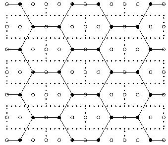
Figure 1: The two-dimensional honeycomb lattice. Solid circles denote the nodes in the lattice, open circles show the unused nodes in the underlying rectangular grid. The dotted lines indicate the unit cells, each of which contains one left- and one right-facing node.

2 A two-dimensional honeycomb lattice

2.1 Geometry of the lattice

We consider the nodes of the hexagonal honeycomb lattice as lying on a subset of a rectangular lattice. First, we introduce orthonormal basis vectors $B=\{\textbf{i},\textbf{j}\}$, where $\textbf{i}=[1,0]^{T}$ and $\textbf{j}=[0,1]^{T}$. The position of the $(m,n)$ node of the rectangular lattice is $m\textbf{i}+hn\textbf{j}$, with $h=\sqrt{3}$ so that the resulting hexagons are regular. In order to specify the honeycomb lattice, we retain only those nodes $(m,n)$ for which $m+n$ is an even integer and omit $m=6p+1$, $n=$ odd and $m=6p+4,n=$ even. In Figure 1 the filled circles denote the nodes retained in the honeycomb lattice which satisfy these relations, and the open circles show all the remaining nodes in the underlying rectangular lattice.

Figure 2: Enlarged view of the honeycomb lattice

To derive governing equations of this lattice we introduce vectors ${\bf e}_{i}=[2,0]^{T}=2{\bf i}$, ${\bf e}_{j}=[-1,h]^{T}=h{\bf j}-{\bf i}$ and ${\bf e}_{k}=[1,h]^{T}={\bf i}+h{\bf j}$, as shown on the right hand side of Figure 2, to describe the two configurations by which nodes are connected to nearest neighbours. The honeycomb lattice is composed of two distinct arrangements of connecting nearest neighbour nodes, shown in Figure 3. We refer to Arrangement 1 as left-facing nodes, since they are connected to a nearest neighbour horizontally to the left. Arrangement 2 will be referred to as right-facing nodes. When looking at Figure 3 we note that each node is connected to three nodes of the opposite arrangement.

Figure 3: Labelling of the nodes in the lattice.

2.2 Derivation of the governing equations

In the application we consider here, at every node there is a nonlinear capacitor, and between adjacent nodes, a linear inductor. We denote the voltage across the capacitor $(m,n)$ by $V_{m,n}$ and the total charge stored on this capacitor by $Q_{m,n}$. Finally, the current in the direction of the vector ${\bf e}_{i}$, through the inductor immediately to the right of $(m,n)$ is denoted by $I_{m,n}$, and $J_{m,n}$ and $K_{m,n}$ represent currents in the direction of the vectors ${\bf e}_{j}$ and ${\bf e}_{k}$, respectively. This configuration is illustrated in Figure 2, which shows an enlarged view of the lattice with the relevant currents indicated.

We derive separate governing equations for the two arrangements of nodes, and only later aim to reconcile the two into a single description. Our aim is to find equations for the variable, $Q_{m,n}$ at each node of the lattice. To enable equations to be derived, we need to make the distinction between left- and right-facing nodes. We use $\widehat{Q}_{m,n}$ for left-facing nodes, that is, arrangement 1 in Figure 3(a), and $\bar{Q}_{m,n}$ for right-facing nodes, namely arrangement 2 in Figure 3(b). We use $Q_{m,n}$ for a general node, in practice, this will be either one of the left-facing ($\widehat{Q}_{m,n}$) or the right-facing ($\bar{Q}_{m,n}$) nodes. A derivation from Kirchoff’s laws has been given in [8]. Here we simply quote the Hamiltonian

$$\widetilde{H} = \!\!\!\sum_{{{m,n;s.t.}\atop{\bar{P}_{m,n}{\rm exists}}}}\!\!\!\mbox{$\frac{1}{2}$}(\bar{P}_{m,n}\!-\!\widehat{P}_{m\!+\!2,n})^{2}+\mbox{$\frac{1}{2}$}(\bar{P}_{m,n}\!-\!\widehat{P}_{m\!-\!1,n\!+\!1})^{2}+\mbox{$\frac{1}{2}$}(\bar{P}_{m,n}\!-\!\widehat{P}_{m\!-\!1,n\!-\!1})^{2}$$ (1)

$$\qquad\qquad+\Upsilon(\bar{Q}_{m,n})+\Upsilon(\widehat{Q}_{m\!+\!2,n}),$$

and note that $P_{m,n}$ and $Q_{m,n}$ are the conjugate momentum and displacement variables of the system. The charge-voltage relationship is given by $V(Q_{m,n})=\Upsilon^{\prime}(Q_{m,n})$ where we assume the potential $\Upsilon(Q_{m,n})$ has the form $\Upsilon(Q)=\mbox{$\frac{1}{2}$}Q^{2}+\mbox{$\frac{1}{3}$}aQ^{3}+\mbox{$\frac{1}{4}$}bQ^{4}$. Since our analysis is based on small amplitude nonlinear expansions, we assume that there is a Taylor series of $\Upsilon(Q)$; we do not consider potentials of the form $\Upsilon(Q)\sim Q^{\nu}$ with $\nu<2$. In Section 4.3 we use the Hamiltonian (1) to find the energy of small amplitude breathers.

The lattice equations are obtained by eliminating $P_{m,n}$ from the equations

$$\frac{dQ_{m,n}}{dt}=\frac{\partial H}{\partial P_{m,n}},\qquad\frac{dP_{m,n}}{dt}=-\frac{\partial H}{\partial Q_{m,n}}=-\Upsilon^{\prime}(Q_{m,n}).$$ (2)

Thus, for left-facing nodes we have

$$\frac{d^{2}\widehat{Q}_{m,n}}{dt^{2}} = \bar{Q}_{m-2,n}+\bar{Q}_{m+1,n-1}+\bar{Q}_{m+1,n+1}-3\widehat{Q}_{m,n}$$ (3)

$$+a\bar{Q}_{m-2,n}^{2}+a\bar{Q}_{m+1,n-1}^{2}+a\bar{Q}_{m+1,n+1}^{2}-3a\widehat{Q}_{m,n}^{2}$$

$$+b\bar{Q}_{m-2,n}^{3}+b\bar{Q}_{m+1,n-1}^{3}+b\bar{Q}_{m+1,n+1}^{3}-3b\widehat{Q}_{m,n}^{3},$$

where $m,n\in{\rm Z\!\!Z}$, $\widehat{Q}_{m,n}$ represents the charge at left-facing nodes and $\bar{Q}_{m,n}$ represents the charge at right-facing nodes. The right-facing nodes in arrangement 2 are governed by

$$\frac{d^{2}\bar{Q}_{m,n}}{dt^{2}} = \widehat{Q}_{m+2,n}+\widehat{Q}_{m-1,n+1}+\widehat{Q}_{m-1,n-1}-3\bar{Q}_{m,n}$$ (4)

$$+a\widehat{Q}_{m+2,n}^{2}+a\widehat{Q}_{m-1,n+1}^{2}+a\widehat{Q}_{m-1,n-1}^{2}-3a\bar{Q}_{m,n}^{2}$$

$$+b\widehat{Q}_{m+2,n}^{3}+b\widehat{Q}_{m-1,n+1}^{3}+b\widehat{Q}_{m-1,n-1}^{3}-3b\bar{Q}_{m,n}^{3}.$$

3 General theory

3.1 Asymptotic analysis

We now aim to find an approximate analytic solution to the equations (3) and (4) by applying the method of multiple scales. We first rescale the current variables $m,n$ and $t$, introducing the new variables

$$X=\varepsilon m,\qquad Y=\varepsilon hn,\qquad\tau=\varepsilon t,\qquad{\rm and}\qquad T=\varepsilon^{2}t,$$ (5)

with $\varepsilon\ll 1$ being the amplitude of the breather, the variables $X,Y$ will be treated as continuous real variables.

We require different ansatzes for the right- and left-facing nodes, therefore we analyse each type of node individually using (3) and (4). For right-facing nodes we seek solutions of the form

$$\bar{Q}_{m,n}(t) = \ {\varepsilon}{\rm e}^{i\psi}F(X,Y,\tau,T)+{\varepsilon}^{2}\left[G_{0}(X,Y,\tau,T)+{\rm e}^{i\psi}G_{1}(X,Y,\tau,T)\right.$$ (6)

$$\left.+{\rm e}^{2i\psi}G_{2}(X,Y,\tau,T)\right]+{\varepsilon}^{3}\left[H_{0}(X,Y,\tau,T)+{\rm e}^{i\psi}H_{1}(X,Y,\tau,T)\right.$$

$$\left.+{\rm e}^{2i\psi}H_{2}(X,Y,\tau,T)+e^{3i\psi}H_{3}(X,Y,\tau,T)\right]+...+c.c.,$$

where the phase of the carrier wave $\psi$ is given by $\psi=km+lhn+\omega t$, where ${\bf k}=[k,l]^{T}$ is the wavevector and $\omega({\bf k})$ is its temporal frequency. Similarly, for left-facing nodes we seek solutions of the form

$$\widehat{Q}_{m,n}(t) = {\varepsilon}e^{i\psi}P+{\varepsilon}^{2}\left[Q_{0}+{\rm e}^{i\psi}Q_{1}+{\rm e}^{2i\psi}Q_{2}\right]$$ (7)

$$+{\varepsilon}^{3}\left[R_{0}+{\rm e}^{i\psi}R_{1}+{\rm e}^{2i\psi}R_{2}+{\rm e}^{3i\psi}R_{3}\right]+...+c.c.,$$

where $P,Q_{j},R_{j}$ are all functions of $(X,Y,\tau,T)$.

After substituting the ansatzes (6) and (7), into the relevant right- and left-facing lattice equations (3) and (4), we equate the coefficients of each harmonic frequency at each order of $\varepsilon$ to find two sets of equations, which we analyse in order below. We use the slightly unusual notation ${\cal O}(\varepsilon^{p}{\rm e}^{iq\psi})$ to mean those terms of ${\cal O}(\varepsilon^{p})$ which have the coefficient ${\rm e}^{iq\psi}$, that is, we neglect those terms which have ${\rm e}^{ir\psi}$ with $r\neq q$.

Since our main calculations are only going as far as ${\cal O}(\varepsilon^{3})$ and ${\cal O}(\varepsilon^{4}{\rm e}^{0i\psi})$, the variables (5) are sufficient for our analysis. At higher orders of $\varepsilon$, we would have to include longer space scales, given by $\widetilde{X}=\varepsilon^{2}m$ and $\widetilde{Y}=\varepsilon^{2}hn$, however, these make little difference to the shape of the breather, as shown in [31].

3.2 ${\cal O}(\varepsilon{\rm e}^{i\psi})$ - the dispersion relation

The first order we investigate is $\cal{O}(\varepsilon{\rm e}^{i\psi})$, whence we obtain

$${\bf M}\left(\begin{array}[]{c}F\\ P\end{array}\right)=\left(\begin{array}[]{cc}3-\omega^{2}&-\beta\\ -\beta^{*}&3-\omega^{2}\end{array}\right)\left(\begin{array}[]{c}F\\ P\end{array}\right)=\bf{0},$$ (8)

where

$$\beta=e^{2ik}+e^{-ik-ilh}+e^{-ik+ilh},$$ (9)

and $\beta^{*}$ is its complex conjugate. We write $\beta=|\beta|{\rm e}^{-i\theta}$, the magnitude being

$$|\beta|=\sqrt{3+2\cos(2lh)+2\cos(3k+lh)+2\cos(3k-lh)}.$$ (10)

We are interested in solutions where $({{F}\atop{P}})\neq\bf{0}$, equation (8) is thus an eigenvalue problem. We require the determinant of the matrix to be zero, which gives the dispersion relation

$$\omega^{2}=3\pm\sqrt{3+2\cos(2lh)+2\cos(3k+lh)+2\cos(3k-lh)}.$$ (11)

The dispersion relation describes the dependence of the temporal frequency of the wave on the wavenumbers $(k,l)$.

The negative square root in (11) leads to an ‘acoustic’ branch, or surface in $(k,l,\omega)$ space with lower frequencies, which we denote by $\omega_{ac}=\sqrt{3-|\beta|}$; and we have $\omega_{ac}\rightarrow 0$ as $k,l\rightarrow 0$. The surface corresponding to the positive root in (11), which clearly has larger values of $\omega$, we denote by $\omega_{opt}=\sqrt{3+|\beta|}$, and we describe this surface as the ‘optical’ branch. The acoustic branch accounts for frequencies in the range $0\leq\omega\leq\sqrt{3}$, whilst the optical branch satisfies $\sqrt{3}\leq\omega\leq\sqrt{6}$.

The plot of $\omega$ against $k$ and $l$ along with the contour plot is shown in Figure 4. We have the dispersion relation (11) for the two coupled systems (3) and (4). We consider $k$ and $l$ such that $(k,l)\in T^{2}=[0,2\pi]\times[0,2\pi/h]$ because $\omega$ is periodic in both $k$ and $l$, with period $2\pi$ in the $k$-direction and period $2\pi/h$ in $l$-direction.

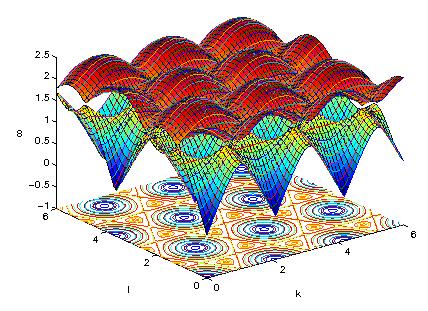
Figure 4: Plot of $\omega$(k), (in colour in online version).

The locations in $(k,l)$ space of the minima of $\omega_{ac}$ and the maxima of $\omega_{opt}$ coincide are seen in Figure 4 as the circles in the centres of the hexagonal shapes in the contour plot. These points are at $(0,0)$, $(2\pi/3,0)$, $(0,2\pi/h)$, $(2\pi/3,2\pi/h)$ and $(\pi/3,\pi/h)$ etc. Points where the two surfaces meet are also evident in Figure 4 as the centres of the triangles surrounding the hexagonal shapes, at these points where $\omega=\sqrt{3}$. The $\omega(k,l)$ dispersion surfaces have cusp-like singularities at these points, which can be denoted by $\bf{k}_{1}$,…,$\bf{k}_{6}$, where

$$\begin{array}[]{rclcrcl}\textbf{k}_{1}&=&[\pi/3,\pi/3h]^{T},&&\textbf{k}_{2}&=&[\pi,\pi/3h]^{T},\\ \textbf{k}_{3}&=&[0,2\pi/3h]^{T},&&\textbf{k}_{4}&=&[0,4\pi/3h]^{T},\\ \textbf{k}_{5}&=&[2\pi/3,2\pi/3h]^{T},&&\textbf{k}_{6}&=&[2\pi/3,4\pi/3h]^{T}.\end{array}$$ (12)

By comparing (11) with (10), we observe that these points occur where $\beta=0$. In graphene, these wavevectors are known as Dirac points [27]. Figure 4 also illustrates the hexagonal symmetry of the lattice. Figure 5 shows the magnitude and argument of $\beta$ as function of $(k,l)$. Note the presence of sizable plateaus where arg$(\beta)\approx 0,\pm 2\pi/3$.

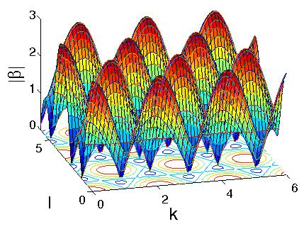
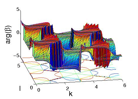
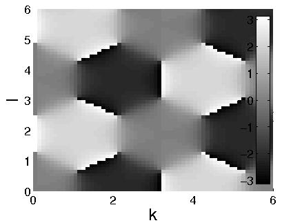
Figure 5: Left: plot of $|\beta|$; centre: plot of arg$(\beta)$, (both in colour in online version); right: greyscale plot of arg$(\beta)$, showing large regions where arg$(\beta)\approx 0,\pm 2\pi/3$.

However, equation (8) remains unsolved. Since det$({\bf M})$=0, solutions can be written as $P=CF$, where, for $\omega_{ac}$ and $\omega_{opt}$, we have

$$C_{ac}=\frac{\beta^{*}}{|\beta|}={\rm e}^{i\theta},\qquad C_{opt}=-C_{ac}=-{\rm e}^{i\theta},$$ (13)

respectively, the latter expression arising from $\beta=\Gamma{\rm e}^{-i\theta}$. These expressions for $C_{ac}$, $C_{opt}$ will be used in later calculations, where we find expressions for the functions $G_{2}$, $G_{1}$, $G_{0}$, $Q_{2}$, $Q_{1}$ and $Q_{0},$ in terms of $F$.

3.3 ${\cal O}(\varepsilon^{2}{\rm e}^{0i\psi})$: relationship between $G_{0}$ and $Q_{0}$

At ${\cal O}(\varepsilon^{2}{\rm e}^{0i\psi})$, we obtain the same equation from both (3) and (4), which are the equations for $\widehat{Q}_{m,n}$ and for $\overline{Q}_{m,n}$.

$$G_{0}+G_{0}^{*}+2a|F|^{2}=Q_{0}+Q_{0}^{*}+2a|P|^{2}.$$ (14)

Note that from the ansatz, $Im(G_{0})$ is irrelevant, since only the combination $G_{0}+G_{0}^{*}$ ever appears in our equations. Hence, we assume $Im(G_{0})=0$, and only consider the real parts, that is, $G_{0}=G_{0}^{*}$. Since $P=CF$ with $|C|=1$, we have $|F|^{2}=|P|^{2}$ in (14), and $G_{0}=Q_{0}$, but this quantity is not yet determined.

3.4 ${\cal O}(\varepsilon^{2}{\rm e}^{2i\psi})$: expressions for $G_{2}$ and $Q_{2}$

As previously mentioned, we aim to express all the variables $G_{0},G_{1},G_{2},Q_{0},Q_{1}$ and $Q_{2}$ in terms of $F$. At $\cal{O}$ $(\varepsilon^{2}e^{2i\psi})$ by substituting the ansatzes (6)–(7) into (3)–(4), we obtain

$$(3-4\omega^{2})G_{2}-\gamma Q_{2} = \gamma aP^{2}-3aF^{2},$$ (15)

$$(3-4\omega^{2})Q_{2}-\gamma^{*}G_{2} = \gamma^{*}aF^{2}-3aP^{2},$$ (16)

where $\gamma^{*}$ is the complex conjugate of $\gamma$ and

$$\gamma=e^{4ik}+e^{-2ik+2ilh}+e^{-2ik-2ilh}.$$ (17)

Note that if we think of $\beta$ and $\gamma$ as being functions of $(k,l)$, they are related by $\gamma(k,l)=\beta(2k,2l)$, compare (9) and (17). Solving the linear system (15)–(16) for $G_{2}$ and $Q_{2}$ as functions of $F$, we find

$$\left(\begin{array}[]{c}G_{2}\\ Q_{2}\end{array}\right)=\frac{aCF^{2}}{(3-4\omega^{2})^{2}-|\gamma|^{2}}\left(\begin{array}[]{c}(|\gamma|^{2}-9+12\omega^{2})C^{*}-4\omega^{2}\gamma C\\ (|\gamma|^{2}-9+12\omega^{2})C-4\omega^{2}\gamma^{*}C^{*}\end{array}\right).$$ (18)

Whilst the bottom term in the vector is the complex conjugate of the top, we do not have $Q_{2}=G_{2}^{*}$ since the the term $CF^{2}$ common to both is not necessarily real. We return to the expressions (18) in Section 5.

3.5 ${\cal O}(\varepsilon^{2}{\rm e}^{i\psi})$: the velocity profile

We now consider the governing equations at ${\cal O}(\varepsilon^{2}{\rm e}^{i\psi})$, which can be written as

$$\textbf{M}\left(\begin{array}[]{c}G_{1}\\ Q_{1}\end{array}\right)=\left(\begin{array}[]{cc}-2i{\omega}F_{\tau}-i\beta_{k}P_{X}-i\beta_{l}P_{Y}\\ -2i{\omega}P_{\tau}-i\beta_{k}^{*}F_{X}-i\beta_{l}^{*}F_{Y}\end{array}\right),$$ (19)

where M is the matrix given in (8), and $\beta_{k}$, $\beta_{l}$ are the partial derivatives of $\beta$ with respect to $k$, $l$ respectively, namely

$$\beta_{k}=2i{\rm e}^{2ik}-i{\rm e}^{-ik-ilh}-i{\rm e}^{-ik+ilh},\qquad\beta_{l}=ih{\rm e}^{-ik+ilh}-ih{\rm e}^{-ik-ilh}.$$ (20)

Since det$({\bf M})=0$, an equation such as (19), which we write as ${\bf M}({{G_{1}}\atop{Q_{1}}})={\bf d}$, either has no solutions, or a whole family of solutions for $(G_{1},Q_{1})^{T}$. According to the Fredholm alternative, the existence of solutions depends on ${\bf d}$. Solutions exist only if the rhs of (19), namely ${\bf d}$, is in the range of the matrix ${\bf M}$, which is given by

$${\rm Range}_{ac} = K\left(\begin{array}[]{c}-\beta\\ |\beta|\end{array}\right)=K\left(\begin{array}[]{c}-{\rm e}^{-i\theta}\\ 1\end{array}\right),$$ (25)

$${\rm Range}_{opt} = K\left(\begin{array}[]{c}\beta\\ |\beta|\end{array}\right)=K\left(\begin{array}[]{c}{\rm e}^{-i\theta}\\ 1\end{array}\right).$$ (30)

Since normals to these directions are given by

$${\bf n}_{ac}=\left(\begin{array}[]{c}{\rm e}^{i\theta}\\ 1\end{array}\right),\qquad{\bf n}_{opt}=\left(\begin{array}[]{c}-{\rm e}^{i\theta}\\ 1\end{array}\right),$$ (31)

the condition that ${\bf d}\in$Range implies ${\bf n.d}=0$. Note that in both the optical and the acoustic cases, (31) implies ${\bf n}=({{C}\atop{1}})$.

We also recall that the leading order quantities, $P$ and $F$ are related by $P=CF$, where both $C$ and ${\bf n}=({{C}\atop{1}})$ have different expressions for the acoustic and optical cases, given by (13). Using $P=CF$ and ${\bf n.d}=0$ we obtain the equation

$$0=4\omega F_{\tau}+(\beta_{k}C+\beta_{k}^{*}C^{*})F_{X}+(\beta_{l}C+\beta_{l}^{*}C^{*})F_{Y}.$$ (32)

This equation implies that $F$ (and hence $P$ as well) is a travelling wave. We write

$$F(X,Y,\tau,T)\equiv F(Z,W,T),\quad{\rm where}\;\;\;Z=X-u\tau,\quad W=Y-v\tau,$$ (33)

the horizontal and vertical velocity components are found to be

$$u = \frac{\beta_{k}C+\beta_{k}^{*}C^{*}}{4\omega}=\frac{-3\sin(3k)\cos(lh)}{\omega|\beta|},$$ (34)

$$v = \frac{\beta_{l}C+\beta_{l}^{*}C^{*}}{4\omega}=\frac{-h\sin(lh)(\cos(3k)+2\cos(lh))}{\omega|\beta|}.$$ (35)

As expected from the standard theory of waves [33] these are simply the derivatives of the frequency with respect to the wavenumber, $u=\partial\omega/\partial k$, $v=\partial\omega/\partial l$. Since we have different expressions for $\omega_{ac}$ and $\omega_{opt}$, equations (34)–(35) also generates different formulae for $u_{ac}$ and $u_{opt}$ (and $v_{ac}$ and $v_{opt}$). Figure 6 shows plots of the horizontal and vertical components of the velocity as functions of the wavenumbers $(k,l)$. Note that at the Dirac points, where $\beta=0$, the singularity is removable since the numerators in (34)–(35) are also zero.

The overall speed, $c$, is given by

$$c = \sqrt{u^{2}+v^{2}}=\frac{h}{\omega|\beta|}\sqrt{\sin^{2}(lh)[\cos(3k)+2\cos(lh)]^{2}+3\sin^{2}(3k)\cos^{2}(lh)},$$

which is plotted in figure 7. Whilst the above calculations, (34)–(LABEL:eqn:avevelocity), are for the acoustic mode, similar calculations for the optical mode produce similar results. All these plots show periodic behaviour, however, the hexagonal symmetry of the system only becomes clear in the total speed, the plots of the velocities $u,v$ have a more complicated, although complimentary form. The velocities $u,v$ both show sensitive dependence on wave vector $(k,l)$. At the wavevectors $\textbf{k}_{1}$,…,$\textbf{k}_{2}$, found in (12), both the components of velocity are zero.

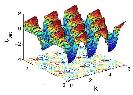
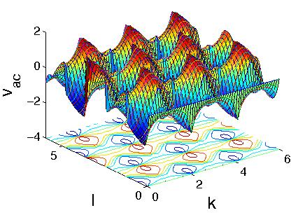
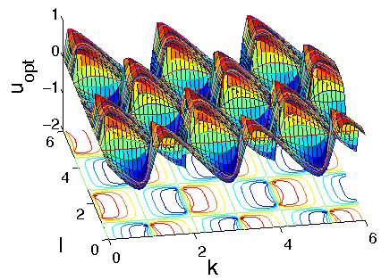
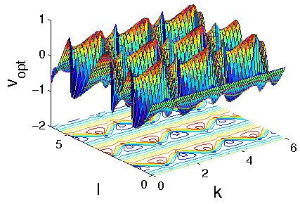
Figure 6: Plot of the horizontal ($u$, on the left) and vertical ($v$, on the right) components of velocity, both as functions of the wavenumbers $k$, $l$; upper row, acoustic mode; lower row, optical mode, (in colour in online version).

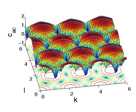
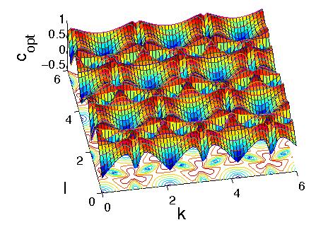
Figure 7: Plot of the total speed as a function of the wavenumbers $(k,l)$; left, acoustic case, right, optical mode, (in colour in online version).

The above calculation gives the condition on the rhs of (19) for solutions to exist. However, the quantities $G_{1}$, $Q_{1}$ remain unknown. The solutions of (19) are degenerate, and the one-parameter family of solutions may be written as

$$\left(\begin{array}[]{c}G_{1}//Q_{1}\end{array}\right)=\left(\begin{array}[]{c}\overline{G}_{1}+\widehat{G}_{1}//C\overline{G}_{1}\end{array}\right),$$ (37)

for arbitrary $\overline{G}_{1}$. The two equations for $\widehat{G}_{1}$ from (19) are then identical, and are solved by

$$\widehat{G}_{1} = \frac{-is}{2|\beta|}\left[(\beta_{k}C-\beta_{k}^{*}C^{*})F_{Z}+(\beta_{l}C-\beta_{l}^{*}C^{*})F_{W}\right],\quad s=\left\{\begin{array}[]{lll}+1&&{\rm acoustic,}\\ -1&&{\rm optical.}\end{array}\right.$$ (40)

Writing this as $\widehat{G}_{1}=\widehat{u}F_{Z}+\widehat{v}F_{W}$, we have

$$\widehat{u}=\frac{2}{|\beta|^{2}}\left[\cos(3k)\cos(lh)-\cos(2lh)\right],\qquad\widehat{v}=\frac{2h}{|\beta|^{2}}\sin(3k)\sin(lh).$$ (42)

Whilst, this leaves $\overline{G}_{1}$ undetermined, the quantity $\widehat{G}_{1}$ describes a small difference in the evolution of the left- and right-handed nodes of the honeycomb lattice.

3.6 ${\cal O}(\varepsilon^{3}{\rm e}^{0i\psi})$: corrections to the slow mode

At ${\cal O}(\varepsilon^{3}{\rm e}^{0i\psi})$, we obtain the equation

$$0=3H_{0}-3R_{0}+3a(F^{*}G_{1}+FG_{1}^{*})-3a(P^{*}Q_{1}+PQ_{1}^{*}),$$ (43)

from the substitution of (6)–(7) into both (3) and (3). We are only interested in determining the leading order terms $\varepsilon F$, $\varepsilon P$, which require the ${\cal O}(\varepsilon^{2})$ terms $G_{0},Q_{0}$, so we do not pursue the determination of $H_{0},R_{0}$, which are ${\cal O}(\varepsilon^{3})$ correction terms and provide only a small difference between the right-facing and left-facing nodes.

3.7 ${\cal O}(\varepsilon^{4}{\rm e}^{0i\psi})$: expressions for $G_{0}$ and $Q_{0}$

In determining $G_{0}$ and $Q_{0}$, in Section 3.3 we found a single relationship at $\cal{O}$ $(\varepsilon^{2}e^{0})$, namely $G_{0}=Q_{0}$. At ${\cal O}(\varepsilon^{3}e^{0})$, we again obtained a single equation; we now move on to consider ${\cal O}(\varepsilon^{4}e^{0})$. Noting that $G_{0}=Q_{0}$ and $G_{0}^{*}=G_{0}$, $|F|^{2}=|P|^{2}$, and consequent results, such as $|G_{2}|^{2}=|Q_{2}|^{2}$, allows significant simplification. Furthermore, the ${\cal O}(\varepsilon^{3}{\rm e}^{i\psi})$ equations analysed below in section 3.8, have the same form as those in Section 3.5, namely, $H_{1},R_{1}$ satisfy a system of the form ${\bf M}({{H_{1}}\atop{R_{1}}})=({{A}\atop{B}})$ for some $A,B$ where ${\bf M}$ is singular. Hence we write the solution for $H_{1},R_{1}$ as $({{H_{1}}\atop{R_{1}}})=({{\overline{H}}\atop{C\overline{H}}})+({{\widehat{H}}\atop{0}})$. Ultimately we obtain the equation for $G_{0}$ as

$$G_{0\tau\tau}=3\nabla^{2}(G_{0}+a|F|^{2})-3a(|\widehat{G}|^{2}+\widehat{G}^{*}\overline{G}+\widehat{G}\overline{G}^{*}+F^{*}\widehat{H}+F\widehat{H}^{*}).$$ (44)

In general, we cannot solve (44) to find $G_{0}$ and $Q_{0}$, but there are two special cases when we can do so. In the cases considered later, either $\widehat{H}=0$ or it is not relevant to our calculations. We also choose $\overline{G}=-\mbox{$\frac{1}{2}$}\widehat{G}$ with (LABEL:hatG1), so that (44) can be simplified to $G_{0,\tau\tau}=3\nabla^{2}(G_{0}+a|F|^{2})$, which is similar to the previously derived results for the square and hexagonal lattices, see equations (2.23) of [7] and (2.23) of [8].

The first special case, analysed in Section 4, is when the interaction potential is symmetric, that is, $V(Q_{m,n})=V(-Q_{m,n})$. Under this assumption, the quadratic coefficient of the force, $a$, is zero, leading to $G_{0}=Q_{0}=0$ as the solution of (44). In this case, we also have $G_{2}=Q_{2}=0$. This means that the system is governed by equations (45)–(47) given below, which can be reduced to a single NLS equation.

In Section 5, we consider the second case, $\omega=\omega_{max}$ where $\omega_{max}$ represents the maxima of $\omega$. In this case the breather is stationary, since (34)–(35) yield $u=0$ and $v=0$, then the system as a whole has no $\tau$-dependence, that is, $P_{\tau\tau}=F_{\tau\tau}=0$. In this case, $G_{0},Q_{0}$ also have no $\tau$-dependence, and so equation (44) reduces to $G_{0}=Q_{0}=-a|F|^{2}$. This solution can be substituted into equations (45)–(47) given below which again can be reduced to a single NLS equation.

3.8 Nonlinear Schrödinger equation

The final equation we need to investigate comes from terms of ${\cal O}(\varepsilon^{3}{\rm e}^{i\psi})$ which yield

$${\bf M}\left(\begin{array}[]{c}H_{1}\\ R_{1}\end{array}\right)=\left(\begin{array}[]{c}A\\ B\end{array}\right),$$ (45)

where the matrix ${\bf M}$ is identical to that in (8), and the rhs components are given by

$$A = -2iwG_{1\tau}-i\beta_{k}Q_{1,X}-i\beta_{l}Q_{1,Y}-2iwF_{T}-F_{\tau\tau}$$ (46)

$$+\mbox{$\frac{1}{2}$}P_{XX}(4{\rm e}^{2ik}+{\rm e}^{-ik+ilh}+{\rm e}^{-ik-ilh})+hP_{XY}({\rm e}^{-ik-ilh}-{\rm e}^{-ik+ilh})$$

$$+\mbox{$\frac{3}{2}$}P_{YY}({\rm e}^{-ik+ilh}+{\rm e}^{-ik-ilh})+3\beta b|P|^{2}P-9b|F|^{2}F$$

$$+2a[\beta(PQ_{0}+PQ_{0}^{*}+P^{*}Q_{2})-3(FG_{0}+FG_{0}^{*}+F^{*}G_{2})],$$

$$B = -2iwQ_{1\tau}-i\beta^{*}_{k}G_{1,X}-i\beta^{*}_{l}G_{1,Y}-2iwP_{T}-P_{\tau\tau}$$ (47)

$$+\mbox{$\frac{1}{2}$}F_{XX}(4{\rm e}^{-2ik}+{\rm e}^{ik-ilh}+{\rm e}^{ik+ilh})+hF_{XY}({\rm e}^{ik+ilh}-{\rm e}^{ik-ilh})$$

$$+\mbox{$\frac{3}{2}$}F_{YY}({\rm e}^{ik-ilh}+{\rm e}^{ik+ilh})+3\beta^{*}b|F|^{2}F-9b|P|^{2}P$$

$$+2a[\beta(FG_{0}+FG_{0}^{*}+F^{*}G_{2})-3(PQ_{0}+PQ_{0}^{*}+P^{*}Q_{2})].$$

As in the case of the equations at ${\cal O}(\varepsilon^{2}{\rm e}^{i\psi})$, in order for this system of equations to have solutions, there is the consistency condition ${\bf n}.({{A}\atop{B}})=0$ that must be satisfied.

An equation for $F(Z,W,T)$ can be obtained from (45)–(47) by the following procedure:
.   (i) calculating the consistency condition ${\bf n}.({{A}\atop{B}})=0$, that is, $CA+B=0$,
.   (ii) substitute in expressions for $G_{2}$, $Q_{2}$, $G_{0}$, $Q_{0}$,
.   (iii) making the substitution $P=CF$,
.   (iv) transforming to travelling wave coordinates by (33).
However, in general, this equation will still be coupled to $G_{0}$, through (44); and carrying out this procedure in general leads to extremely lengthy expressions.

3.9 Summary

We have derived a multiple scales asymptotic expansion for envelope solutions of the scalar two-dimensional honeycomb lattice. After finding the usual expressions for the frequency, and group velocity, we have found a coupled system of PDEs for the shape of the envelope given by (44) and (45)–(47). Whilst we cannot, in general, solve this resulting system of equations, there are two special cases in which the system reduces to a single NLS equation. The general case shares some similarities with the Davey-Stewartson system of equations [11] obtained in fluid mechanics. The remainder of this paper is not directed to a general analysis of equations (44) and (45)–(47), rather we consider two special cases in more detail.

These two cases are considered in more detail in Sections 4 and 5 respectively, and in both cases the procedure (i)–(iv) leads to substantially simpler expressions than the general case. In both special cases we find additional criteria which, if not satisfied, mean the the lattice cannot support breather solutions.

4 The symmetric potential ($a=0$) and moving breathers

In this Section we consider the simplified case where $a=0$ in (3) and (4) so that $V(-\phi)=V(\phi)$ and $V^{\prime}(-\phi)=-V^{\prime}(\phi)$. In section 3.4, whilst equation (18) remains valid, we recover $G_{2}=Q_{2}=0$, that is, there is no generation of second harmonics. Furthermore, from Section 3.7 we gain $G_{0}=0=Q_{0}$, which satisfies the relationship $G_{0}=Q_{0}$ from Section 3.3. This means that there is no ‘slow’ mode, which is independent of $t$ (corresponding to $\omega=0$), and the localised mode evolves only on the slower $\tau,T$ timescales.

4.1 ${\cal O}(\varepsilon^{3}{\rm e}^{i\psi})$ - derivation of NLS

We now apply the procedure (i)–(iv) from Section 3.8 and so simplify the NLS-like system (19)–(47). Taking $G_{1}$, $Q_{1}$ as given by (37) with $\overline{G}=-\mbox{$\frac{1}{2}$}\widehat{G}$ and using $P=CF$ to evaluate ${\bf n}.({{A}\atop{B}})=0$, we obtain a single equation for $F$, namely

$$0 = -4iwF_{T}-2F_{\tau\tau}+\mbox{$\frac{1}{2}$}F_{XX}\left[C(4{\rm e}^{2ik}+{\rm e}^{-ik+ilh}+{\rm e}^{-ik-ilh})\right.$$ (48)

$$\left.+C^{*}(4{\rm e}^{-2ik}+{\rm e}^{ik-ilh}+{\rm e}^{ik+ilh})\right]$$

$$+hF_{XY}\left[C({\rm e}^{-ik-ilh}-{\rm e}^{-ik+ilh})+C^{*}({\rm e}^{ik+ilh}-{\rm e}^{ik-ilh})\right]$$

$$+\mbox{$\frac{3}{2}$}F_{YY}\left[C({\rm e}^{-ik+ilh}+{\rm e}^{-ik-ilh})+C^{*}({\rm e}^{ik-ilh}+{\rm e}^{ik+ilh})\right]$$

$$+3b|F|^{2}F(\beta C+\beta^{*}C^{*}-6).$$

Thus we have completed stages (i)–(iii) of the procedure from Section 3.8. In stage (iv) we eliminate the $\tau$-derivative terms using the travelling wave substitution $F(X,Y,\tau,T)=F(Z,W,T)$ with $u$ and $v$ representing the horizontal and vertical components of velocity found in (34)–(35). Using $F_{\tau\tau}=u^{2}F_{ZZ}+2uvF_{ZW}+v^{2}F_{WW}$, we rewrite (48) as

$$4iwF_{T} = D_{Z}F_{ZZ}+D_{W}F_{WW}+D_{M}F_{WZ}+3b|F|^{2}F(\beta C+\beta^{*}C^{*}-6),$$ (49)

where

$$\Delta_{Z} \!=\! \frac{2}{|\beta|}\left[4\cos(2lh)+5\cos(lh)\cos(3k)\right],\qquad\Delta_{M}=\frac{4h}{|\beta|}\sin(3k)\sin(lh),$$

$$\Delta_{W} \!=\! \frac{6}{|\beta|}\cos(lh)\left[\cos(3k)+2\cos(lh)\right],$$ (50)

$$\begin{array}[]{rclcrcl}D_{Z,ac}&=&\Delta_{Z}-2u_{ac}^{2}-|\beta|\widehat{u}^{2},&&D_{Z,opt}&=&-\Delta_{Z}-2u_{opt}^{2}+|\beta|\widehat{u}^{2},\\ D_{W,ac}&=&\Delta_{W}-2v_{ac}^{2}-|\beta|\widehat{v}^{2},&&D_{W,opt}&=&-\Delta_{W}-2v_{opt}^{2}+|\beta|\widehat{v}^{2},\\ D_{M,ac}&=&-\Delta_{M}-4u_{ac}v_{ac}-|\beta|\widehat{u}^{2},&&D_{M,opt}&=&\Delta_{M}-4u_{opt}v_{opt}+2|\beta|\widehat{u}\widehat{v}.\end{array}$$ (54)

(55)

Hence, from the governing equations (3)–(4), we have found (49), which is an NLS equation in 2+1 dimensions.

4.2 The elliptic NLS equation

To make further progress towards understanding the form of possible solutions of the system (49)–(55), we make the substitution

$$\zeta=\lambda Z,\qquad\xi=W-\frac{D_{M}Z}{2D_{Z}},$$ (56)

to remove the mixed derivative term. This transformation yields

$$4iwF_{T}=D_{Z}\left(\lambda^{2}F_{\zeta\zeta}+\frac{(4D_{W}D_{Z}-D_{M}^{2})}{4D_{Z}^{2}}F_{\xi\xi}\right)+3b|F|^{2}F(\beta C+\beta^{*}C^{*}-6).$$ (57)

The NLS equation in 2+1 dimensions has two forms depending on whether the second-differential operator part of the equation is elliptic or hyperbolic. We are only interested in elliptic systems (where the coefficients of $F_{\xi\xi}$ and $F_{\zeta\zeta}$ have have the same sign) as our aim is to find solutions which are localised in both spatial dimensions. We therefore define the ellipticity as

$${\cal E}(k,l)=4D_{W}D_{Z}-D_{M}^{2},\qquad\lambda=\frac{\sqrt{{\cal E}}}{2D_{Z}},$$ (58)

where expressions for $D_{W}$, $D_{Z}$ and $D_{M}$ are given in (50)–(55). Since we have two expressions for $C$, one for the acoustic mode and the other for the optical mode, as given in (13), we have different expressions for $D_{Z}$, $D_{W}$, $D_{M}$ in the two cases, and two expressions for the ellipticity, ${\cal E}_{ac}$ and ${\cal E}_{opt}$.

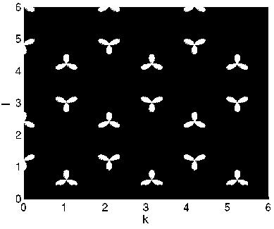
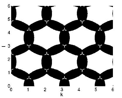
Figure 8: Left: plots of the region where the function ${\cal E}_{ac}(k,l)>0$, showing this to be negative almost everywhere (dark areas), only positive in small areas near the Dirac points (marked in white); right: plot of the region where ${\cal E}_{opt}(k,l)$ is positive (white), showing large areas, around maxima of the frequency $\omega_{opt}$, (eg $(k,l)=(0,0)$) and small areas near the Dirac points.

In Figure 8 we plot the sign of the ellipticity functions ${\cal E}(k,l)$ from (58) for the acoustic and optical cases. In the acoustic case, ${\cal E}_{ac}\leq 0$ for almost all $(k,l)$, there being small trefoil-shaped areas of positive ellipticity near the Dirac points. However, for the optical case, there is a wide range of wavenumbers where ${\cal E}_{opt}>0$, as shown by the white hexagonal areas in the right panel of Figure 8. Note that the optical case also shows small trefoil-shaped areas of positive ellipticity near the Dirac points. Breathers corresponding to these wavenumbers are expected to be unstable as their frequencies will coincide with those of linear waves. Whilst the dispersion relation in this diatomic system does not have a gap – the frequency spectrum $\omega(k,l)$) includes all values from zero to $\omega_{{\rm max}}=\sqrt{3}$, the form of the breathers near the Dirac points are expected to be similar to those of gap solitons in other diatomic systems, where the dispersion relation has gaps. One-dimensional FPU problems have been studied by Livi et al. [21] and James & Noble [17]. As in one-dimensional diatomic systems, the breathers corresponding to the optical domain including $(k,l)=(0,0)$ have frequencies which lie above the optical band, and so are expected to be long-lived.

We now focus the optical case, where $C=C_{opt}=-{\rm e}^{i\theta}$, and (57) simplifies to

$$4i\omega F_{T}=\lambda^{2}D_{Z}\nabla^{2}_{(\xi,\zeta)}F-6b(3+|\beta|)|F|^{2}F.$$ (59)

In order for bright breathers to exist, there is a second criterion to be satisfied, namely that the coefficients of the nonlinear term and the spatial derivative must have the same sign. Since the nonlinearity is negative, we require $D_{Z}<0$. For the optical mode, this condition is satisfied for all $(k,l)$.

4.3 Asymptotic estimates for breather energy

The total electrical energy in the honeycomb lattice is conserved. This quantity is related to the Hamiltonian (1) by $E=\widetilde{H}/C_{0}$. Thus, upto quadratic order,

$$H=C_{0}E = \mbox{$\frac{1}{2}$}\sum_{m,n}\widehat{Q}_{m+2,n}^{2}+\overline{Q}_{m,n}^{2}+(\overline{P}_{m,n}-\widehat{P}_{m+2,n})^{2}+(\overline{P}_{m,n}-\widehat{P}_{m-1,n-1})^{2}$$ (60)

$$\qquad+(\overline{P}_{m,n}-\widehat{P}_{m-1,n+1})^{2}.$$

Now our aim is to work out an expression for energy at leading order in $\varepsilon$, given our solution for $\widehat{Q}$, $\overline{Q}$ in terms of $F$. Since we are only interested in leading order approximation to the energy, the dependence of the solution for $F$ given by (68) on $T$ can be ignored, as the dependence on $\omega$ dominates. However, in passing we note that from (68) that the combined frequency of the breather mode is given by

$$\Omega=\omega+\frac{3b\varepsilon^{2}A^{2}(3+|\beta|)}{4\omega},$$ (61)

and so, in the optical case, the frequency lies above the frequency of linear waves. From (6)–(7) we find

$$\overline{Q}_{m,n} = 2\varepsilon A\phi(r)\cos(km+lhn+\omega t),$$

$$\widehat{Q}_{m,n} = -2\varepsilon A\phi(r)\cos(km+lhn+\omega t+\theta),$$ (62)

where $r$ is given by the argument of $\phi$ in (68), and using $P=CF=-{\rm e}^{i\theta}F$ since we are considering optical modes. For both left- and right-facing nodes, $\widehat{Q}_{m,n}$ and $\overline{Q}_{m,n}$, we have ${\rm d}^{2}Q/{\rm d}t^{2}=-\omega^{2}Q$, and ${\rm d}P/{\rm d}t=-Q$; hence, at leading order, ${\rm d}Q/{\rm d}t=\omega^{2}P$ and

$$\overline{P}_{m,n} = -\frac{2\varepsilon A}{\omega}\phi(r)\sin(km+lhn+\omega t),$$

$$\widehat{P}_{m,n} = \frac{2\varepsilon A}{\omega}\phi(r)\sin(km+lhn+\omega t+\theta).$$ (63)

The equation for the energy is given by (60), here we show the calculation of the onsite ($\widehat{Q}_{m,n}$, $\overline{Q}_{m,n}$) part of this, the calculation of the interaction energy (due to $\overline{P}_{m,n}$, $\widehat{P}_{m,n}$) can be found in a similar way and gives an identical final expression.

We replace the double sum over $(m,n)$ in (60) by an integral over $(X,Y)$-space using (5), and transform into an integral over $(Z,W)$-space using (33). The Jacobian required to then make the transformation from $(Z,W)$ to $(\xi,\eta)$ coordinates using (56) is $\left|\frac{\partial(\xi,\eta)}{\partial(Z,W)}\right|=\lambda$. Hence

$$2C_{0}E \!=\sum_{{{m,n\ \rm{s.t.}}\atop{\overline{Q}_{m,n}\rm{exists}}}}\overline{Q}_{m,n}^{2}+\widehat{Q}_{m+2,n}^{2}=\int\int 4A^{2}\phi^{2}\frac{{\rm d}Z{\rm d}W}{h}=\frac{2\pi I{\cal E}}{3bh(3+|\beta|)},$$ (64)

where $I:=\int_{0}^{\infty}r\phi^{2}(r)\,{\rm d}r$. The final stages use $r=(A/\lambda)\sqrt{(\xi^{2}+\zeta^{2})3b(3+|\beta|)/(-D_{z})}$ and (58). The above calculation makes use of the result $\sum_{m,n}\phi^{2}(r)\cos(km+lhn+\omega t)=0$ since $r$ is slowly varying in $m,n$.

From equation (64), we note that to leading order, the energy of the breather is independent of the breather amplitude, $A$. Thus, no matter how small the breather amplitude, there is a minimum energy required to create it. The reason for this threshhold energy is that as the amplitude reduces, the width of the breather increases, in such a way that the total energy remains constant. This property confirms the observations of Flach et al. in [15].

However, the threshold energy is dependent on the wavenumbers $k$ and $l$, therefore moving breathers have different threshold energies. Figure 9 shows that the energy threshold is locally maximised at $k=l=0$, that is, for static breathers. Moving breathers require less energy to form. An alternative viewpoint is that as breathers lose energy, they start moving, and accelerate, to the maximum speed, where the ellipticity constraint is only just satisfied. It is also clear from (64) that the energy is closely related to the ellipticity constraint. Finally, we note that the breathers predicted near the Dirac points, which have frequencies lying in the linear spectrum, have much higher energies than the out-of phase optical breathers whose frequencies lie above the top of the linear spectrum.

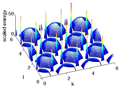
Figure 9: Plot of $-\lambda D_{Z}/(3+|\beta|)$ against $(k,l)$, this being the ($k,l$)-dependent part of the breather energy $E(k,l)$ (64), (in colour in online version).

5 Static breathers in an asymmetric potential

In this Section we examine the more general case for which $a\neq 0$ in (3) and (4). Recall that at the end of Section 3 we obtained a system of two coupled equations for $G_{0}$ and $F$, namely (44) and the equation that can be derived by following the procedure (i)–(iv) in Section 3.8. It is only possible to reduce this system to a single solvable equation when $a=0$ (as analysed above in Section 4) and when $G_{0}$ is independent of $\tau$, which we discuss in this section.

The only example where the system becomes independent of $\tau$ is the case $k=l=0$, on the optical branch. Under these conditions, we have, from (9), (11), (13), (20), (34), (35), (33), (42)

$$\beta=3,\quad\theta=0,\quad\omega_{opt}=\sqrt{6},\quad C=-1,\quad\beta_{k}=\beta_{l}=0,\quad u=v=c=0,$$

$$Z\equiv X,\quad W\equiv Y,\quad\widehat{u}=\widehat{v}=0.$$ (65)

Since $u=v=0$, in this case, the breather is stationary; in addition, from (18), we find ($\gamma=3$ and) $G_{2}=Q_{2}=0$. Assuming $G_{0}$ is independent of $\tau$, equation (44) can be solved by $G_{0}=Q_{0}=-a|F|^{2}$, enabling us to perform stage (ii) of the process outlined in Section 3.8.

Now we turn to deriving the NLS equation. From stage (i) in Section 3.8, and since $C=-1$, we form the equation $A=B$ from (46)–(47). Since $P=-F$, stage (iii) of the calculation leads to

$$2i\sqrt{6}F_{T}+3(F_{XX}+F_{YY})+6(3b-4a^{2})|F|^{2}F=0.$$ (66)

For bright breather solutions to exist, we require the coefficients of the nonlinearity and the spatial diffusion terms to have same signs, that is, $b>\mbox{$\frac{4}{3}$}a^{2}$. In place of (61), the breather’s frequency is now given by $\Omega=\sqrt{6}+3\varepsilon^{2}A^{2}(3b-4a^{2})/2\sqrt{6}$, which still lies above the top of the phonon band.

5.1 ${\cal O}(\varepsilon^{3}{\rm e}^{3i\psi})$: expression for the third harmonic

As noted above, the second harmonic terms, $G_{2}$ and $Q_{2}$ are both zero for the case of stationary breathers, that is the optical mode with $k=l=0$. Hence we extend the expansion of Section 3 to consider the terms at ${\cal O}(\varepsilon^{3}{\rm e}^{3i\psi})$ to see if third harmonic terms are generated. At ${\cal O}(\varepsilon^{3}{\rm e}^{3i\psi})$, we obtain similar equations to those of Section 3.4, more specifically we obtain

$$-9\omega^{2}H_{3} = ({\rm e}^{6ik}+{\rm e}^{-3ik+3ilh}+{\rm e}^{-3ik-3ilh})(R_{3}+bP^{3}+2aPQ_{2})-3H_{3}$$

$$-3bF^{3}-6aFG_{2},$$

$$-9\omega^{2}R_{3} = ({\rm e}^{-6ik}+{\rm e}^{3ik-3ilh}+{\rm e}^{3ik+3ilh})(H_{3}+bF^{3}+2aFG_{2})-3R_{3}$$ (67)

$$-3bP^{3}-6aPQ_{2}.$$

These are the equations for general $k,l$; however, for stationary breathers we are only concerned with $k=l=0$, in which case $Q_{2}=G_{2}=0$, $\omega=\sqrt{6}$ and $P=-F$, hence we obtain the solution $H_{3}=\mbox{$\frac{1}{8}$}bF^{3}$, $R_{3}=-\mbox{$\frac{1}{8}$}bF^{3}$. Thus we find that the honeycomb lattice generates third harmonics but not second harmonics in the stationary breather.

5.2 Comparison with other lattice geometries

In earlier papers [7, 8] we have carried out similar calculations on the square and hexagonal lattices, where the derivations are considerably simpler. In all cases we have $G_{0}=-a|F|^{2}$; however, other properties of the lattices differ, depending on the geometries concerned. In Table 1 we compare the results of the honeycomb lattice analysed here with corresponding results for the square and hexagonal lattices analysed earlier.

Property  $\backslash$  Geometry	Square [7]	Hexagonal [8]	Honeycomb
Second harmonic	$G_{2}=0$	$G_{2}=\mbox{$\frac{1}{3}$}aF^{2}$	$G_{2}=Q_{2}=0$
Third harmonic	$H_{3}=\mbox{$\frac{1}{8}$}bF^{3}$	$H_{3}=0$	$H_{3}=-R_{3}=\mbox{$\frac{1}{8}$}bF^{3}$
Inequality relating nonlin coeff	$b>\mbox{$\frac{4}{3}$}a^{2}$	$b>\frac{10}{9}a^{2}$	$b>\frac{4}{3}a^{2}$

Table 1: Table summarising various properties of the different lattice geometries.

The absence of any second harmonic is a property shared with the square lattice. Whilst the hexagonal lattice generates no third harmonic, it does generate a second harmonic. Furthermore, the inequality relating the coefficients of nonlinear terms is identical for the honeycomb lattice and the square lattice, whilst different for the hexagonal. The possibly surprising result from this table is that, at least as far as stationary breathers are concerned, the honeycomb lattice has more in common with the square lattice than the hexagonal lattice.

5.3 Stability of the breather

The solution for $F$ is a one-parameter family, which we parametrise by the amplitude, $A$, as

$$F=A\exp\left(\frac{3ibA^{2}T(3+|\beta|)}{4\omega}\right)\phi\left(\frac{A}{\lambda}\sqrt{\frac{3b(3+|\beta|)(\xi^{2}+\zeta^{2})}{-D_{Z}}}\right),$$ (68)

where $\phi(r)$ is the function which solves the elliptic problem $\nabla^{2}\phi=\phi-\phi^{3}$in two dimensions. This elliptic problem is known to have solutions, and the cylindrically-symmetric solution we write as $\phi(r)$. Solutions such as (68) are known as Townes soliton solutions [10] of the 2D NLS. These solutions are known to be unstable in the two-dimensional NLS, with subcritical initial conditions suffering from dispersion, leading to the amplitude converging to zero everywhere through the initial data spreading out; whilst supercritical initial conditions blow up, with the energy being focused to a single point, where the amplitude diverges. However, arbitrarily small structural perturbations to (59) can stabilize the Townes soliton. For example, results proven by Davydova et al. [12] for the equation

$$iF_{T}+D\nabla^{2}F+B|F|^{2}F+P\nabla^{4}F+K|F|^{4}F=0,$$ (69)

demonstrate the stability of a localised breather mode if $BD>0$ and $PK>0$. Clearly the presence of a higher derivative terms can mollify the blow-up singularity, whilst higher order nonlinearities can also help stabilise the soliton, as discussed by Kuznetsov [19].

If we pursue higher order correction terms, for example, from ${\cal O}(\varepsilon^{5}{\rm e}^{i\psi})$ terms, then terms such as $\nabla^{4}F$ and $|F|^{4}F$ occur, which may stabilise the Townes soliton provided their coefficients have the correct combinations of signs. However, such an expansion also yields terms of the form $\nabla^{2}(|F|^{2}F)$, $|F|^{2}\nabla^{2}F$ and $F^{2}\nabla^{2}F^{*}$, and the effect of such structural perturbations of (59) has, to our knowledge, not yet been determined. Fibich and Papanicolaou [13, 14] have also addressed this problem, though their results do not yet extend to these nonlinear derivative terms.

To illustrate this, let us consider the case of stationary breathers on a symmetric lattice, that is, we take the nearest-neighbour restoring force to be $V^{\prime}(\phi)=\phi+b\phi^{3}+g\phi^{5}$ (that is, $a=0$ and no quartic nonlinearity). We analyse the special case given by $k=l=0$, so that $u=v=0$, $G_{0}=Q_{0}=Q_{2}=G_{2}=0$. Note that we also have $\widehat{u}=\widehat{v}=0$ so that $\widehat{G}=0$, $H_{0}=R_{0}$ and we can take $\overline{G}=0$ so that $G_{1}=Q_{1}=0=H_{0}=R_{0}=0$. Hence, in place of the ansatzes (6)–(7), used earlier, we use the simplified forms

$$\overline{Q}=\varepsilon{\rm e}^{i\psi}F+\varepsilon^{3}{\rm e}^{3i\psi}H_{3}+\varepsilon^{5}\sum_{j=1}^{5}{\rm e}^{ij\psi}J_{j}, \widehat{Q}=\varepsilon{\rm e}^{i\psi}P+\varepsilon^{3}{\rm e}^{3i\psi}R_{3}+\varepsilon^{5}\sum_{j=1}^{5}{\rm e}^{ij\psi}U_{j},$$

with $H_{3}=\mbox{$\frac{1}{8}$}bF^{3}$, and $R_{3}=-\mbox{$\frac{1}{8}$}bF^{3}$ as derived in Section 5.1. Our aim is to calculate the form of the higher-order terms, namely those at ${\cal O}(\varepsilon^{4}{\rm e}^{i\psi})$ and ${\cal O}(\varepsilon^{4}{\rm e}^{i\psi})$.

Combining the results from ${\cal O}(\varepsilon{\rm e}^{i\psi})$, ${\cal O}(\varepsilon^{3}{\rm e}^{i\psi})$, ${\cal O}(\varepsilon^{5}{\rm e}^{i\psi})$, we obtain the governing equations

$$(3\!-\!\omega^{2})\varepsilon F+\varepsilon^{5}J_{1})-3(\varepsilon P+\varepsilon^{5}U_{1})$$ (71)

$$= -2i\omega\varepsilon^{3}F_{T}+3\varepsilon^{3}\nabla^{2}P+9b\varepsilon^{3}(|P|^{2}P-|F|^{2}F)-\varepsilon^{5}F_{TT}$$

$$-2i\omega\varepsilon^{5}F_{\widetilde{T}}+\varepsilon^{4}(P_{XXX}-3P_{XYY})+\mbox{$\frac{3}{4}$}\varepsilon^{5}\nabla^{4}P+6\varepsilon^{5}\nabla.\widetilde{\nabla}P$$

$$+3b\varepsilon^{5}\nabla^{2}(|P|^{2}P)+\varepsilon^{5}(30g+\mbox{$\frac{9}{8}$}b)(|P|^{4}P-|F|^{4}F),$$

$$-3(\varepsilon F+\varepsilon^{5}J_{1})+(3\!-\!\omega^{2})(\varepsilon P+\varepsilon^{5}U_{1})$$ (72)

$$= -2i\omega\varepsilon^{3}P_{T}+3\varepsilon^{3}\nabla^{2}F+9b\varepsilon^{3}9(|F|^{2}F-|P|^{2}P)-\varepsilon^{5}P_{TT}$$

$$-2i\varepsilon^{5}\omega P_{\widetilde{T}}+\varepsilon^{4}(-F_{XXX}+3F_{XYY})+\mbox{$\frac{3}{4}$}\varepsilon^{5}\nabla^{4}F+6\varepsilon^{5}\nabla.\widetilde{\nabla}F$$

$$+3b\varepsilon^{5}\nabla^{2}(|F|^{2}F)+\varepsilon^{5}(30g+\mbox{$\frac{9}{8}$}b)(|F|^{4}F-|P|^{4}P).$$

Here, in addition to the long scales defined in (5), we have introduced even longer time and length scales given by $\widetilde{T}=\varepsilon^{4}t$, $\widetilde{X}=\varepsilon^{3}m$, and $\widetilde{Y}=\varepsilon^{3}hm$, and $\widetilde{\nabla}$ is the corresponding vector derivative with respect to $\widetilde{X}$ and $\widetilde{Y}$.

Since $\omega=\sqrt{6}$, the right-hand-sides of (71)–(72) must be equal. Combining this with the relation $P=-F$ leads to

$$0 = 2i\sqrt{6}(F_{T}+\varepsilon^{2}F_{\widetilde{T}})+3\nabla^{2}F+18b|F|^{2}F$$

$$+\varepsilon^{2}\left[F_{TT}+\mbox{$\frac{3}{4}$}\nabla^{4}F+6\nabla.\widetilde{\nabla}F+3b\nabla^{2}(|F|^{2}F)+(60g+\mbox{$\frac{9}{4}$}b^{2})|F|^{4}F\right],$$

since the third-derivative terms cancel. Whilst these terms generate nonzero solutions for $J_{1},U_{1}$, such contributions do not concern us here, where our aim is to determine the properties of $F$. The effect of the $F_{\widetilde{T}}$ term is to change the timescale slightly, and the $\nabla.\widetilde{\nabla}F$ term rescales the space scale $X$, hence we will neglect these terms.

Applying $2i\omega\partial_{T}$ to the leading order form of (5.3), which is (66) in the case $a=0$, yields

$$0=8F_{TT}+3\nabla^{4}F+108b^{2}|F|^{4}F+18b(\nabla^{2}(|F|^{2}F)+2|F|^{2}\nabla^{2}F-F^{2}\nabla^{2}F^{*}),$$ (74)

which we use to eliminate $F_{TT}$ from (5.3), to find the final governing equation

$$0 = 2i\sqrt{6}F_{T}+3\nabla^{2}F+18b|F|^{2}F+\mbox{$\frac{3}{8}$}\varepsilon^{2}\nabla^{4}F+(60g-\mbox{$\frac{45}{4}$}b^{2})\varepsilon^{2}|F|^{4}F$$ (75)

$$+\mbox{$\frac{3}{4}$}b\varepsilon^{2}\nabla^{2}(|F|^{2}F)+\mbox{$\frac{9}{4}$}b\varepsilon^{2}F^{2}\nabla^{2}F^{*}-\mbox{$\frac{9}{2}$}b\varepsilon^{2}|F|^{2}\nabla^{2}F.$$

As the last three terms do not appear in (69), we cannot formally determine the stability properties of the system. However, if we were to simply ignore the last three terms, (69) suggests that if $g>\mbox{$\frac{3}{16}$}b^{2}$ (and $b>0$) then the combined influence of the fifth-order nonlinearities and fourth order derivatives stabilise the breather. Since we expect that the second derivatives of cubic nonlinearities can be bound by some combination of fifth order nonlinearities and fourth order derivatives of $F$, it is reasonable to assume that for sufficiently large $g$, the breather will be stable.

6 Conclusions

We have investigated the properties of discrete breathers on a two-dimensional honeycomb lattice. After applying Kirchoff’s laws to the electrical lattice, we derived a governing set of equations for the case of nonlinear capacitors at nodes, and nodes being connected by linear inductors. Using multiple scales asymptotic methods, we reduced the governing equations to a single NLS equation from which we can determine the properties and conditions under which small-amplitude breathers may exist. There are two cases in which an NLS equation can be obtained. We analysed each case in more detail in Sections 4 and 5.

The analysis of the honeycomb is more complicated than either the square or the triangular lattices, due to the necessity of treating the two types of node, which means that a diatomic analysis must be carried out. This leads to extra complications at the level of determining the evolution of the ‘slow mode’ at ${\cal O}(\varepsilon^{4}{\rm e}^{0})$. Part of the extra complexity is that in order to derive the leading order $F$ and $P$ terms in (6) and (7), it is necessary to simultaneously find the first correction terms $G_{1}$ and $Q_{1}$.

The first special case we considered (§4) was that of a symmetric potential in which the terms $G_{0}$, $Q_{0}$, $Q_{2}$ and $G_{2}$ are all zero. From this we were able to obtain an ellipticity condition, for the wavenumbers $(k,l)$, to ensure we obtained solutions which were localised in both spatial directions. A minimum threshold energy to create breathers was also found. This confirmed the observations of Flach et al. [15]. The ellipticity condition, breather energy and dispersion relation, obtained in Sections 3.2 and 4, were plotted. The breather energy is maximised for these stationary breathers. For other wave vectors, moving breathers are created, with lower energies.

The second case we analysed was the case of asymmetric potentials. Here we only considered the specific wavenumber $k=l=0$, and the optical branch which guarantees stationary breathers. However, this enabled us to describe the behaviour of a range of nonlinearity parameters ($a,b$) for which stationary breathers may exist. We find no second harmonic term in the expansion in this case, but there is a third harmonic. These properties show a close similarity between the square lattice and the honeycomb, quite distinct from the hexagonal lattice.

It is natural to consider the relationship between the honeycomb system studied here and a one-dimensional systems. We note that the two-dimensional systems studied previously [7, 8] both had a dispersion relation with a single branch that described modes with optical and acoustic characters, as in one-dimensional (monatomic) systems. However, in one-dimensional diatomic systems, the dispersion relation has two branches, one optical and one acoustic. Such systems have been studied by Livi et al. [21] and James & Noble [17], amongst others. In the latter paper, the authors derive the dispersion relation, showing it to have two branches: an optical and an acoustic form, as in the honeycomb lattice. However, in the one-dimensional diatomic lattice, the two branches are distinct, and do not meet at Dirac points; rather, there is a gap between the two branches, in which breathers may exist with frequencies which are not coincident with any linear wave. In the honeycomb lattice, the two branches meet at the Dirac points, and so there is no gap. However, from Figure 8 we see that the honeycomb lattice still supports breather solutions near the Dirac points. Whilst it would be interesting to investigate these solutions further, we expect them to be unstable, since their frequencies coincide with those of linear waves, allowing energy interchange with phonons which could lead to the breather’s decay. In contrast, we now consider the larger white regions in Figure 8 (right), corresponding to wavenumbers for which optical breathers exist. We expect these breathers to have frequencies above the top of the optical band, and so will have no linear wave with the same frequency. These waves, however, may still be unstable, due to other effects, such as the breather’s motion over lattice sites being resonant with linear modes. Such losses may still allow the breather to travel long distances before decaying, and so be relevant in applications such as the explanation of tracks in mica via quodons as suggested by Russell and Eilbeck [29, 28].

In this paper we have only looked at a scalar-valued quantities at each node that is, only one degree of freedom. In future works we aim to analyse the stability of these breather solutions, and find approximate solutions to the vector-valued honeycomb lattice similar to the lattices Marin et al. studied in [24].

Acknowledgements

We are grateful to Hadi Susanto for useful conversations.

References

References

- [1]
- [2] MJ Ablowitz and Y Zhu. Nonlinear waves in shallow honeycomb lattices. SIAM J. Appl. Math., 72, 240–260, (2012).
- [3] O Bahat-Treidel, O Peleg, M Segev and H Buljan. Breakdown of Dirac dynamics in honeycomb lattices due to nonlinear interactions. Phys. Rev. A, 82, 013830, (2010).
- [4] J Bajar and JAD Wattis. in preparation (2013).
- [5] D Bonart, AP Mayer, and U Schröder. Anharmonic localised surface vibrations in a scalar model, Phys. Rev. B. 51, 13739 (1995).
- [6] VM Burlakov, SA Kiselev, and VN Pyrkov. Computer simulation of intrinsic localized modes in one-dimensional and two-dimensional anharmonic lattices, Phys. Rev. B 42, 4921 (1990).
- [7] IA Butt and JAD Wattis. Discrete breathers in a two-dimensional Fermi-Pasta-Ulam lattice. J Phys A: Math Gen, 39, 4955, (2006).
- [8] IA Butt and JAD Wattis. Discrete breathers in a hexagonal two-dimensional Fermi-Pasta-Ulam lattice, J Phys A: Math Theor, 40, 1239, (2007).
- [9] AP Chetverikov, W Ebeling and MG Velarde. Localized nonlinear, soliton-like waves in two-dimensional anharmonic lattices. Wave Motion 48, 753–760, (2011)
- [10] RY Chiao, E Garmine and CH Townes. Self-trapping of optical beams Phys. Rev. Lett. 13, 479 (1964).
- [11] A Davey, K Stewartson. On three dimensional packets of surface waves. Proc. R. Soc. A 338, 101–110 (1974).
- [12] TA Davydova, AI Yakimenko and YA Zaliznyak. Two-dimensional solitons and vortices in normal and anomalous dispersive media. Phys. Rev. E, 67, 026402, (2003).
- [13] G Fibich and G Papanicolaou. A modulation method for self-focusing in the perturbed critical nonlinear Schrödinger equation. Phys. Lett. A, 239, 167, (1998) .
- [14] G Fibich & G Papanicolaou. Self-focusing in the perturbed and unperturbed nonlinear Schrödinger equation in critical dimension SIAM J. Appl. Math., 60, 183, (1999).
- [15] S Flach, K Kladko and RS MacKay. Energy thresholds for discrete breathers in one-,two-, and three-dimensional lattices, Phys. Rev. Lett. 78, 1207, (1997).
- [16] S Flach, K Kladko and CR Willis. Localised excitations in two-dimensional Hamiltonian lattices Phys Rev E, 50, 2293, (1994).
- [17] G James and P Noble. Breathers on diatomic Fermi-Pasta-Ulam lattices. Physica D, 196, 124–171, (2004)
- [18] PG Kevrekidis, BA Malomed and YuB Gaididei. Solitons in triangular and honeycomb dynamical lattices with the cubic nonlinearity. Phys Rev E, 66, 016609, (2002)
- [19] EA Kuznetsov, AM Rubenchik and VE Zakharov. Soliton stability in plasmas and hydrodynamics. Phys. Rep., 142, 103, (1986).
- [20] A Leonard, C Chong, PG Kevrekedis and C Daraio. Traveling waves in 2D hexagonal granular crystal lattices. arXiv.org/nlin.PS/1305.0171
- [21] R Livi, M Spicci, RS MacKay. Breathers on a diatomic FPU chain. Nonlinearity, 10, 1421–1434, (1997)
- [22] RS MacKay and J-A Sepulchre. Effective Hamiltonian for travelling discrete breathers, J. Phys. A.: Math.Gen. 35, 3958 (2002).
- [23] RS MacKay and S Aubry. Proof of existence of breathers for time-reversible or Hamiltonian networks of weakly coupled oscillators, Nonlinearity 7, 1623 (1994).
- [24] JL Marin, JC Eilbeck and FM Russell. Localised moving breathers in a 2D hexagonal lattice, Phys. Lett. A. 248, 225 (1998).
- [25] JL Marin, JC Eilbeck and FM Russell. Breathers in cuprate-like lattices, Phys Lett A, 281, 21, (2001).
- [26] MI Molina and YS Kivshar. Discrete and surface solitons in photonic graphene nanoribbons. Optics Letters, 35, 2895, (2010).
- [27] O Pegel, G Bartal, B Freedman, O Manela, M Segev and DN Christodoulides. Conical diffraction and gap solitons in honeycomb photonic lattices. Phys Rev Lett, 98, 103901, (2007).
- [28] FM Russell. Indentification and selection criteria for charged lepton tracks in mica, Nucl. Tracks Radiat. Meas., 15, 41 (1998).
- [29] FM Russell and JC Eilbeck. Evidence for moving breathers in a layered crystal insulator at 300K. Europhys. Lett. 78, 1005–, (2007).
- [30] S Takeno. Localized modes in the long-time behavior of anharmonic lattices, J. Phys. Soc. Japan. 59, 1571 (1990).
- [31] JAD Wattis. Stationary breather modes of generalized nonlinear Klein-Gordon lattices. J. Phys. A; Math. Gen., 31, 3301–3323, (1998).
- [32] X Yi, JAD Wattis, H Susanto, L Cummings. Discrete breathers in a two-dimensional spring-mass lattice. J Phys A; Math Theor, 42, 355207, (26pp), (2009).
- [33] GB Whitham. Linear and Nonlinear Waves. Wiley, New York, (1974).