Effective field theories on solitons of generic shapes

Abstract

A class of effective field theories for moduli or collective coordinates on solitons of generic shapes is constructed. As an illustration, we consider effective field theories living on solitons in the O(4) non-linear sigma model with higher-derivative terms.

1 Introduction

Effective field theory is one of the most useful tools available to date. Even the standard model, although renormalizable in its present formulation, may also be just an effective theory of Nature where possible supersymmetric and/or grand unified extensions have been integrated out. For particles of accessible energies, we can neglect gravity and consider particles on flat space as a(n extremely) good approximation. This is just a consequence of the separation of scales between the particle mass and energy versus the scale of gravity, i.e. the Planck mass. Light fields do not only exist in all of spacetime but are sometimes confined to certain subspaces. For solitons hosting moduli, there is again a situation where separation of scales can be exploited; namely the mass of the soliton versus massless or light moduli. Effective field theories for moduli have been constructed for many kinds of solitons, but very often only in cases where the soliton has a simple, flat or straight shape. As examples, the effective actions for monopole moduli [1], domain-wall moduli [2, 3, 4, 5] and for orientational moduli of non-Abelian strings [6, 4, 5, 7] have been constructed. When solitons are particle-like such as monopoles this can describe the low-energy dynamics of the solitons in a compact way as geodesics of moduli spaces [1], while for solitons being extended objects such as domain walls or vortices, this describes field theories on their world-volume, as in the case of D-branes in string theory or more general branes. Solitons can, however, generically possess much more complicated shapes.

In this Letter we construct a first attempt of effective field theories in principle applicable to solitons of generic shapes and apply it to a class of models possessing soliton solutions of flat, spherical, cylindrical and toroidal shapes.

2 General considerations

Here we will consider a generalized framework where we expand a set of fields in eigenmodes as [2]

$$\Phi^{a}=\sum_{n}\mathcal{M}_{n}(\mathbf{e}_{\alpha})\zeta_{n}^{a}(\mathbf{e}_{i}),$$ (1)

where $\zeta_{n}$ are eigenfunctions, $\mathcal{M}_{n}$ are moduli fields, while $\mathbf{e}_{\alpha}$ and $\mathbf{e}_{i}$ are sets of vectors in transverse (world-volume) dimensions ($\alpha=0,1,\ldots t$) and codimensions ($i=t+1,\ldots t+c$), respectively, of a soliton of a generic shape; see Fig. 1. For simplicity we consider only flat space in this Letter and we have made a decomposition of directions (locally) as $\mathbb{R}^{d,1}=\mathbb{R}^{t,1}\times\mathbb{R}^{c}$, where the $d=c+t$ spatial dimensions are split into $c$ codimensions and $t$ transverse dimensions.

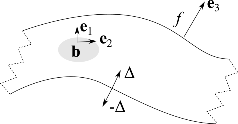
Figure 1: Sketch of a generic soliton profile in direction $\mathbf{e}_{3}$. The moduli $\mathbf{b}$ live on the manifold spanned by the host soliton. The integration over the codimension is done only over a finite range $[-\Delta,\Delta]$, allowing for a generic shape of the host soliton.

The kinetic term in the underlying theory will give rise to a kinetic term for the moduli as

$$\int_{\mathbf{e}_{i}}|\nabla_{\mu}\Phi|^{2}\supset|\nabla_{\mathbf{e}_{\alpha}}\mathcal{M}_{n}|^{2}\int_{\mathbf{e}_{i}}|\zeta_{n}|^{2}\propto\frac{1}{M^{c}}|\nabla_{\mathbf{e}_{\alpha}}\mathcal{M}_{n}|^{2},$$ (2)

where $M$ is a characteristic mass of the soliton system and $\mu$ are all spacetime indices. For higher-order derivative terms, one similarly obtains e.g.,

$$\int_{\mathbf{e}_{i}}|\nabla_{\mu}\Phi|^{2}|\nabla_{\nu}\Phi|^{2}\supset|\nabla_{\mathbf{e}_{\alpha}}\mathcal{M}_{n}|^{2}\int_{\mathbf{e}_{i}}\left|\nabla_{\mathbf{e}_{i}}\zeta_{m}\right|^{2}|\zeta_{n}|^{2}$$

$$\quad\propto\frac{1}{M^{c-2}}|\nabla_{\mathbf{e}_{\alpha}}\mathcal{M}_{n}|^{2}.$$ (3)

Notice the relative enhancement of this term compared to that of (2). The higher-order term induces an enhanced kinetic term in the low-energy effective theory living on the soliton.

However, the lower-order term also induces other terms in the low-energy effective theory, which will be of higher-order. These induced terms are of a different kind as they are higher-order corrections coming from integrating out massive modes propagating on the soliton. Let us consider the kinetic term, which would induce something like

$$\frac{1}{M^{c+2}}|\nabla_{\mathbf{\alpha}}\mathcal{M}_{n}|^{2}|\nabla_{\mathbf{\alpha^{\prime}}}\mathcal{M}_{n^{\prime}}|^{2}.$$ (4)

This higher-order correction in the effective theory is naturally suppressed by (2 powers of) the soliton scale. Whether this term will be comparable to the higher-order terms in the theory before we take the low-energy limit on the soliton depends on the theory and the parameters.

In this Letter, we consider the higher-order terms to be numerically significant and work in the limit of very high soliton mass, where we safely can neglect the higher-order corrections coming from lower-order terms.

Let us comment on integrating out the host soliton. We assume that the soliton is extended in the directions spanned by $\{\mathbf{e}_{i}\}$ which is taken to be orthogonal to $\{\mathbf{e}_{\alpha}\}$. However, integrating over all the subspace spanned by $\{\mathbf{e}_{i}\}$ may be problematic; but for physical reasons we need only integrate over the major energy peak of the soliton solution (say in the range $[-\Delta,\Delta]$) on which the moduli live and thus neglect the long tales that the soliton may possess; see fig. 1. We do this for physically capturing the low-energy effective theory on the soliton and in a way that we can still use the decomposition of the transverse and world-volume coordinates locally.

Finally, we need to assess the quality of the approximation we are making, since we are taking into account corrections proportional to powers of the soliton mass coming from higher-order terms. The approximation we are making is a separation of scales between the mass of the host soliton and the energies of the moduli in the effective action living on the world-volume. The higher-order terms, if they have non-negligible coefficients, induce lower-order terms in the low-energy effective theory on the soliton which are enhanced by a factor of $(M/m)^{\delta d}$ (where $\delta d$ is the difference in dimension between the higher-order term and the lower-order term while $m$ is the typical scale of the moduli). On the other hand, as mentioned above, the lower-order terms also induce higher-order correction terms which come about from integrating out massive modes propagating along the soliton. These terms are, however, suppressed by a factor of $(m/M)^{2}$ (or higher). It has also been assumed all along that the derivatives in the low-energy effective theory are not too large. As long as the ratio $m/M$ is sufficiently small, we can use just the leading-order low-energy effective theory.

Higher-order corrections coming from the lower-order terms, as mentioned above, can however be calculated systematically [7], but we will not consider them in this Letter; i.e., here we present only the leading-order effective action.

3 Non-linear sigma model

To illustrate our framework more explicitly, we will now specialize the considerations presented above to an O(4)-sigma model with higher-derivative terms in $3+1$ flat dimensions, which has scalar fields, $n^{a}$, of an O(4) vector, with $a=1,\ldots,4$ and Lagrangian density

$$\mathcal{L}=-m^{4}V+c_{2}m^{2}\mathcal{L}_{2}+c_{4}\mathcal{L}_{4}+\frac{c_{6}}{m^{2}}\mathcal{L}_{6}+\cdots$$ (5)

where $\mathcal{L}_{n}$ is the Lagrangian density containing the $n$-th order derivative terms

$$-\mathcal{L}_{2} =\frac{1}{2}\partial_{\mu}\mathbf{n}\cdot\partial^{\mu}\mathbf{n},$$ (6)

$$-\mathcal{L}_{4} =\frac{1}{4}\big{(}\partial_{\mu}\mathbf{n}\cdot\partial^{\mu}\mathbf{n}\big{)}^{2}-\frac{1}{4}\big{(}\partial_{\mu}\mathbf{n}\cdot\partial_{\nu}\mathbf{n}\big{)}^{2},$$ (7)

$$\mathcal{L}_{6} =\mathcal{B}_{\mu}\mathcal{B}^{\mu},\quad\mathcal{B}^{\mu}=\frac{1}{6}\epsilon^{\mu\nu\rho\sigma}\epsilon^{abcd}\partial_{\nu}n^{a}\partial_{\rho}n^{b}\partial_{\sigma}n^{c}n^{d},$$ (8)

and $\mathcal{B}^{\mu}$ is the baryon current. Finally, an appropriate potential should be chosen for the soliton under study. There still remains a choice to be made, i.e. the codimension of the soliton under consideration. Since we consider $\mathbb{R}^{3,1}$ here, there are only two non-trivial cases: a codimension-one soliton like a domain wall or a codimension-two soliton like a vortex. We will study each in turn in the following.

3.1 Codimension-one case

We will now consider the soliton of the type which is described by a codimension-one field $\zeta(\mathbf{e}_{3})$ and two moduli $\mathcal{M}_{1,2}(\mathbf{e}_{1},\mathbf{e}_{2})$, where the condensate field is a function of the direction spanned by the vector $\mathbf{e}_{3}$ only and the moduli are functions of two orthogonal directions $\mathbf{e}_{1}$ and $\mathbf{e}_{2}$. For concreteness we will parametrize the non-linear sigma-model field, $\mathbf{n}$, as

$$\mathbf{n}=\{\mathbf{b}\sin f,\cos f\},$$ (9)

where $\mathbf{b}$ are scalar fields of a unit 3-vector ($\mathbf{b}\cdot\mathbf{b}=1$) describing two moduli and is a function only of the orthogonal directions to the field $f$, i.e. $\mathbf{b}(\mathbf{e}_{1},\mathbf{e}_{2})$. The domain solution also possesses a position modulus, which we will not take into account in this Letter. Taking the Lagrangian densities (6-8) one-by-one, choosing the potential

$$m^{2}V=-\frac{1}{2}m_{3}^{2}n_{3}^{2}+\frac{1}{2}M^{2}(1-n_{4}^{2}),$$ (10)

and integrating over the codimension spanned by $\mathbf{e}_{3}$, we get

$$-\mathcal{L}_{2}^{\rm eff} =\frac{a_{2,0}^{\alpha\alpha^{\prime}}}{M}\partial_{\alpha}\mathbf{b}\cdot\partial_{\alpha^{\prime}}\mathbf{b},\quad m^{2}V^{\rm eff}=-\frac{a_{2,0}m_{3}^{2}}{M}b_{3}^{2},$$

$$-\mathcal{L}_{4}^{\rm eff} =a_{2,2}^{\alpha\alpha^{\prime}}M\,\partial_{\alpha}\mathbf{b}\cdot\partial_{\alpha^{\prime}}\mathbf{b}$$

$$\phantom{=}+\frac{a_{4,0}^{\alpha\alpha^{\prime}\beta\beta^{\prime}}}{2M}\big{(}\partial_{\alpha}\mathbf{b}\times\partial_{\beta}\mathbf{b}\big{)}\cdot\big{(}\partial_{\alpha^{\prime}}\mathbf{b}\times\partial_{\beta^{\prime}}\mathbf{b}\big{)},$$

$$-\mathcal{L}_{6}^{\rm eff} =a_{4,2}^{\alpha\alpha^{\prime}\beta\beta^{\prime}}M\big{(}\partial_{\alpha}\mathbf{b}\times\partial_{\beta}\mathbf{b}\big{)}\cdot\big{(}\partial_{\alpha^{\prime}}\mathbf{b}\times\partial_{\beta^{\prime}}\mathbf{b}\big{)},$$ (11)

where we have defined the dimensionless constants as follows

$$a_{k,\ell}^{\alpha_{1}{\alpha_{1}}^{\prime}\ldots\alpha_{n}{\alpha_{n}}^{\prime}}\equiv$$

$$\frac{M}{2}\int_{\mathbf{e}_{3}}\sqrt{\det h}\;\sin^{k}f\left(\frac{\partial_{\mathbf{e}_{3}}f}{M}\right)^{\ell}h^{\alpha_{1}{\alpha_{1}}^{\prime}}\cdots h^{\alpha_{n}{\alpha_{n}}^{\prime}},$$ (12)

where $h^{\alpha\alpha^{\prime}}$ is the inverse induced metric on the surface of the host soliton. Note that to leading order which we consider here, the induced metric is diagonal.

The least surprising result is the kinetic term giving back the kinetic term for the moduli with the normalization constant of the effective Lagrangian being $1/M$. The Skyrme term gives also back a Skyrme term for the moduli, but in addition it induces again a kinetic term for the moduli, however enhanced by a factor of $M^{2}$. Finally and perhaps most interestingly, the sixth-order derivative term induces only the (baby-)Skyrme term for the moduli and nothing else.

Putting the pieces together, we have

$$-\mathcal{L}^{\rm eff}=\left(\frac{c_{2}a_{2,0}^{\alpha\alpha^{\prime}}m}{M}+\frac{c_{4}a_{2,2}^{\alpha\alpha^{\prime}}M}{m}\right)m\;\partial_{\alpha}\mathbf{b}\cdot\partial_{\alpha^{\prime}}\mathbf{b}$$

$$+\left(\frac{c_{4}a_{4,0}^{\alpha\alpha^{\prime}\beta\beta^{\prime}}m}{2M}+\frac{c_{6}a_{4,2}^{\alpha\alpha^{\prime}\beta\beta^{\prime}}M}{m}\right)$$

$$\times\frac{1}{m}\big{(}\partial_{\alpha}\mathbf{b}\times\partial_{\beta}\mathbf{b}\big{)}\cdot\big{(}\partial_{\alpha^{\prime}}\mathbf{b}\times\partial_{\beta^{\prime}}\mathbf{b}\big{)}-\frac{a_{2,0}m_{3}^{2}m^{2}}{M}b_{3}^{2}.$$ (13)

There are now three mass scales in the game: the domain wall mass $M$, the length scale of the sector that has generated the kinetic terms, $m$, and finally the mass term for the moduli $m_{3}$. Symmetry breaking requires that $m_{3}\ll M$; this is also needed in order for the scales of the moduli to be much smaller than that of the host soliton. The total energy of the domain wall is $E_{\rm DW}=2\sqrt{c_{2}}Mm^{2}A$, where $A$ is the area of the domain wall and the thickness of the domain wall is $L_{\rm DW}=1/M$. Hence in order for the moduli to be really localized, we need $M$ larger than the other scales in the problem, in particular $M\gg m$ (or more precisely $\sqrt{c_{6}}M\gg\sqrt{c_{4}}m$). In this limit, we can neglect the first term in each parenthesis of (13).

Let us comment on the higher-order corrections from the lower-order terms due to integration out of massive modes. The kinetic term will induce higher-order corrections of order $(m^{2}/M^{3})$, which in our regime of parameters will be small compared to the leading-order terms that we have given here, which are of orders $1/M$ and $M/m^{2}$, respectively. As long as the ratio $m/M$ is sufficiently small, our leading-order low-energy effective theory on the soliton is a good approximation.

Let us further comment on leaving out the position moduli from the low-energy effective action. The position moduli are first of all not as interesting as the orientational moduli, in the physical context we have in mind here. Second, once the host soliton is curved, the position moduli acquire a mass of the order of the curvature scale and are thus subleading with respect to the orientational part. Let us however remark that the higher-order corrections coming from the kinetic term generically induce a mixing term between the position and orientation moduli at the fourth order in derivatives. These higher-order corrections can, however, be systematically calculated using the approach of Ref. [7].

The domain wall can host a so-called baby-Skyrmion [8], which can be identified with a Skyrmion [9] in the bulk [10, 11] (lower dimensional analogues of this correspondence can be found in Ref. [12].)

Using a scaling argument [13], we can estimate the size of the baby-Skyrmion on the flat domain wall as $1/L\sim\sqrt{m_{3}/M}m$, and as $M\gg m_{3}$ it is always relatively large in units of $1/m$ (this estimate holds also for vanishing $c_{4}$).

If $c_{6}$ is very small or vanishes, the size estimate of the baby-Skyrmion on the flat domain wall in the large-$M$ limit becomes $1/L\sim\sqrt{m_{3}m}$, and so is independent of the thickness of the host domain wall.

3.1.1 Example 1: flat domain wall

The sine-Gordon kink is an exact solution to the equations of motion derived from the Lagrangian density (5) with the field parametrization (9)

$$f=2\arctan\exp(\pm Mx/\sqrt{c_{2}}).$$ (14)

This solution is exact when the moduli, $\mathbf{b}$ are (any) constants. Due to separation of scales, we can still use this soliton shape as a good approximation even when the moduli do possess dynamics. The full solutions have been obtained in Ref. [11].

A vast simplification in this example is that the induced metric is just the flat metric, so the effective Lagrangian coefficients, $a$, do not depend on the Greek indices. We can thus evaluate the coefficients in the effective Lagrangian

$$a_{k,\ell} =\frac{1}{2}c_{2}^{(1-\ell)/2}\int_{-\Delta M/\sqrt{c_{2}}}^{\Delta M/\sqrt{c_{2}}}dy\;{\rm sech}^{k+\ell}y.$$ (15)

If we define, $a_{k+\ell}\equiv a_{k,\ell}\,c_{2}^{(\ell-1)/2}$, we have

$$a_{k+\ell} =\frac{1}{2}\sinh y\left.{}_{2}F_{1}\left(\frac{1}{2},\frac{1+k+\ell}{2},\frac{3}{2},-\sinh^{2}y\right)\right|_{-\frac{\Delta M}{\sqrt{c_{2}}}}^{\frac{\Delta M}{\sqrt{c_{2}}}},$$

where ${}_{2}F_{1}$ is a hypergeometric function. If we take the limit of $\Delta M\to\infty$, the constants are $a_{2}=1$, $a_{4}=2/3$, and $a_{6}=8/15$. $a_{2n}=\sqrt{\pi}\,\Gamma(n)/\Gamma(n+1/2)$, with $n\in\mathbb{Z}_{>0}$ a positive integer, takes value in $(0,1]$ and is monotonically decreasing with $n$. For the flat domain wall case, we can finally write down the effective Lagrangian density

$$-\mathcal{L}^{\rm eff} =\left(\frac{c_{2}^{\frac{3}{2}}a_{2}m}{M}+\frac{c_{4}a_{4}M}{\sqrt{c_{2}}m}\right)m\big{(}\partial_{\alpha}\mathbf{b}\big{)}^{2}$$

$$+\left(\frac{\sqrt{c_{2}}c_{4}a_{4}m}{2M}+\frac{c_{6}a_{6}M}{\sqrt{c_{2}}m}\right)\frac{1}{m}\big{(}\partial_{\alpha}\mathbf{b}\times\partial_{\beta}\mathbf{b}\big{)}^{2}$$

$$-\frac{\sqrt{c_{2}}a_{2}m^{2}m_{3}^{2}}{M}b_{3}^{2},$$ (16)

where the world-volume directions are $\{\mathbf{e}_{\alpha}\}=\{y,z\}$.

3.1.2 Example 2: spherical domain wall

This is the first non-flat example. Let us begin with a word of caution. Our construction focuses on the effective description of the moduli on a soliton of a given shape. It does not guaranty stability or even existence of the host soliton. These questions are a separate issue and should be addressed carefully and independently. A further issue is that not all topological sectors of the moduli are available in the effective theory. In this case of a spherical domain wall; the moduli have to live in the topological charge-one sector. Full solutions have been constructed in the literature [14].

Here we will simply assume the form of the spherical domain wall with size $R$ and construct the effective theory that would live on such an object. $R$ will however be a function of the parameters in the theory as it is actually determined dynamically. The induced inverse metric is $\{h^{rr},h^{\theta\theta},h^{\phi\phi}\}=\{1,R^{2}/r^{2},R^{2}/r^{2}\sin^{2}\theta\}$, and $\sqrt{\det h}=(r/R)^{2}\sin\theta$, where we have rescaled the induced metric so that it is dimensionless. The constants of the effective Lagrangian can be determined from (12). Finally, we can write the effective Lagrangian in this case

$$- \mathcal{L}^{\rm eff}=m\sin\theta\left[c_{2}mR\tilde{a}_{2,0,0}+\frac{c_{4}}{mR}\tilde{a}_{2,2,0}\right]$$

$$\phantom{=+}\times\left((\partial_{\theta}\mathbf{b})^{2}+\frac{1}{\sin^{2}\theta}(\partial_{\phi}\mathbf{b})^{2}\right)$$

$$\phantom{=}+\frac{m}{\sin\theta}\left[\frac{c_{4}}{mR}\tilde{a}_{4,0,-2}+\frac{2c_{6}}{(mR)^{3}}\tilde{a}_{4,2,-2}\right]$$

$$\phantom{=+}\times\big{(}\partial_{\theta}\mathbf{b}\times\partial_{\phi}\mathbf{b}\big{)}^{2}-(mR)^{2}Rm_{3}^{2}\sin\theta\tilde{a}_{2,0,2}b_{3}^{2},$$ (17)

where the integration measure now is simply $d\theta d\phi$ and the following dimensionless constants have been defined

$$\tilde{a}_{k,\ell,n}\equiv\frac{1}{2}\int dy\;y^{n}\sin^{k}f(y)(\partial_{y}f)^{\ell},\quad y\equiv\frac{r}{R}.$$ (18)

In this example we will not contemplate taking any limits, as the system is somewhat complicated. The size of the sphere, $R$, is dynamically determined and is a function of the other parameters in the theory, e.g. $c_{2},c_{4},c_{6},m,M$ and so on.

3.2 Codimension-two case

The final type of soliton we will consider is of codimension two and is described by two fields, $f(\mathbf{e}_{2},\mathbf{e}_{3})$, $g(\mathbf{e}_{2},\mathbf{e}_{3})$ and a single modulus $\mathcal{M}(\mathbf{e}_{1})$, where the modulus lives in a single dimension only (plus time). We will parametrize the non-linear sigma-model field, $\mathbf{n}$, as

$$\mathbf{n}=\{\sin f\cos g,\sin f\sin g,\mathbf{b}\cos f\},$$ (19)

where $\mathbf{b}$ are scalar fields of a unit 2-vector ($\mathbf{b}\cdot\mathbf{b}=1$) describing an $S^{1}$ modulus and is a function orthogonal to both the fields of the host soliton $f,g$, i.e. $\mathbf{b}(\mathbf{e}_{1})$. We take again the Lagrangian densities (6-8), choose the potential

$$m^{2}V=-\frac{1}{2}m_{3}^{2}n_{3}^{p_{3}}+m^{2}V_{\rm vortex},$$ (20)

where $p_{3}=1,2$ and integrate over the codimensions $\mathbf{e}_{2}$ and $\mathbf{e}_{3}$ to obtain

$$-\mathcal{L}_{2}^{\rm eff} =\frac{a_{2,0,0}^{\alpha\alpha^{\prime}}}{M^{2}}\partial_{\alpha}\mathbf{b}\cdot\partial_{\alpha^{\prime}}\mathbf{b},$$ (21)

$$-\mathcal{L}_{4}^{\rm eff} =a_{2,1,0}^{\alpha\alpha^{\prime}}\;\partial_{\alpha}\mathbf{b}\cdot\partial_{\alpha^{\prime}}\mathbf{b},$$ (22)

$$-\mathcal{L}_{6}^{\rm eff} =2a_{2,0,2}^{\alpha\alpha^{\prime}}M^{2}\;\partial_{\alpha}\mathbf{b}\cdot\partial_{\alpha^{\prime}}\mathbf{b},$$ (23)

$$m^{2}V^{\rm eff} =-\frac{a_{p_{3},0,0}m_{3}^{2}}{M^{2}}b_{1}^{p_{3}},$$ (24)

which are all Lagrangians for a free (massive) theory for the modulus. The non-trivial part however is the content of the coefficients

$$a_{p,k,\ell}^{\alpha_{1}{\alpha_{1}}^{\prime}\ldots\alpha_{n}{\alpha_{n}}^{\prime}}\equiv\frac{M^{2-2k-2\ell}}{2}$$

$$\times\int_{\mathbf{e}_{2},\mathbf{e}_{3}}\sqrt{\det h}\;\cos^{p}f\left[(\nabla_{\mathbf{e}_{i}}f)^{2}+\sin^{2}f(\nabla_{\mathbf{e}_{i}}g)^{2}\right]^{k}$$

$$\phantom{\times\int_{\mathbf{e}_{2},\mathbf{e}_{3}}\ }\times\left[\sin f\epsilon^{ij}\nabla_{\mathbf{e}_{i}}f\nabla_{\mathbf{e}_{j}}g\right]^{\ell}h^{\alpha_{1}{\alpha_{1}}^{\prime}}\cdots h^{\alpha_{n}{\alpha_{n}}^{\prime}}.$$ (25)

Let us first put together the pieces of the effective Lagrangian density

$$-\mathcal{L}^{\rm eff} =\left(\frac{c_{2}a_{2,0,0}^{\alpha\alpha^{\prime}}m^{2}}{M^{2}}+c_{4}a_{2,1,0}^{\alpha\alpha^{\prime}}+\frac{2c_{6}a_{2,0,2}^{\alpha\alpha^{\prime}}M^{2}}{m^{2}}\right)$$

$$\phantom{=+\ }\times\partial_{\alpha}\mathbf{b}\cdot\partial_{\alpha^{\prime}}\mathbf{b}-\frac{a_{p_{3},0,0}m^{2}m_{3}^{2}}{M^{2}}b_{1}^{p_{3}}.$$ (26)

The first term (21) gives just a kinetic term for the modulus with a standard prefactor, while the second term (22) gives the kinetic term but with a relative enhancement by a factor proportional to the kinetic energy of the host soliton. Finally, and perhaps most interestingly, the last term (23) gives again a kinetic term for the modulus, but with a prefactor proportional to the baby-Skyrmion charge of the orthogonal $S^{2}$ to the $S^{1}$ where the modulus lives. For some host solitons, this charge may vanish of course.

Let us again comment on the higher-order corrections from the lower-order terms due to integration out of massive modes. The first correction will be a fourth-order term and thus it will not compete with any terms given here.

3.2.1 Example 3: straight vortex

In the straight vortex case, we consider a non-trivial soliton in the fields $f,g$ and the $S^{1}$ modulus extending in the $z$ direction. For this we can choose the potential

$$m^{2}V_{\rm vortex}=\frac{1}{2}M^{2}(n_{1}^{2}+n_{2}^{2})(n_{3}^{2}+n_{4}^{2}),$$ (27)

and the coefficients can easily be evaluated. For the straight vortex the only metric-component entering the coefficient is $h^{zz}=1$ which is trivial and the integrals can be carried out numerically in cylindrical coordinates using $\det h=\rho^{2}$ and the polar derivatives, i.e. $(\nabla f)^{2}=f_{\rho}^{2}+f_{\theta}^{2}/\rho^{2}$. The effective Lagrangian density thus reads

$$-\mathcal{L}^{\rm eff} =\left(\frac{c_{2}a_{2,0,0}m^{2}}{M^{2}}+c_{4}a_{2,1,0}+\frac{2c_{6}a_{2,0,2}M^{2}}{m^{2}}\right)(\partial_{z}\mathbf{b})^{2}$$

$$\phantom{=}-\frac{a_{p_{3},0,0}m^{2}m_{3}^{2}}{M^{2}}b_{1}^{p_{3}}.$$ (28)

This effective theory possesses sine-Gordon kinks. For instance, for $p_{3}=1$ a baby-Skyrmion string extended in the $z$ direction can bear sine-Gordon kinks in terms of its twisted $S^{1}$ modulus and each of these kinks can be interpreted in the full 3-dimensional theory as Skyrmions. Setting $p_{3}=2$ results in half-kinks which correspond in the full 3-dimensional theory to half-Skyrmions (possessing half the baryon charge of that of a Skyrmion).

The final example is to compactify the vortex on a circle to obtain a vorton [15, 16]. In this case, the effective Lagrangian is basically the same as the above one, with the kinetic term replaced by $(\partial_{\theta}\mathbf{b})^{2}$ and of course different, but straightforward to compute, coefficients $a$. In this case, the twisting of the modulus implies that only full Skyrmions exist (and thus no half-Skyrmions).

4 Discussion

We have developed a basic framework for calculating effective actions on, in principle, generic solitons. The advantage of this approach is the simplified theories for the types of objects a host soliton can host. The disadvantage is that stability and existence should be carefully examined separately. In this work we did not consider the translational type of moduli, which is related with the shape itself of the soliton as this is a somewhat more complicated problem; we thus leave this part for future developments. Needless to say, one can calculate higher-order classical corrections to these effective actions and finally one may consider also quantum corrections etc. A different generalization that would be interesting to consider for GUT-scale solitons is to take the curvature of spacetime into account; this can be seen as the next-level geometric backreaction.

Acknowledgments

The work of MN is supported in part by Grant-in-Aid for Scientific Research (No. 25400268) and by the “Topological Quantum Phenomena” Grant-in-Aid for Scientific Research on Innovative Areas (No. 25103720) from the Ministry of Education, Culture, Sports, Science and Technology (MEXT) of Japan. SBG thanks Keio University for hospitality where this work was carried out. SBG also thanks the Recruitment Program of High-end Foreign Experts for support.

References

- [1] N. S. Manton, Phys. Lett. B 110, 54 (1982); M. F. Atiyah and N. J. Hitchin, Phys. Lett. A 107, 21 (1985); G. W. Gibbons and N. S. Manton, Phys. Lett. B 356, 32 (1995) [hep-th/9506052].
- [2] B. Chibisov and M. A. Shifman, Phys. Rev. D 56, 7990 (1997) [Erratum-ibid. D 58, 109901 (1998)] [hep-th/9706141].
- [3] Y. Isozumi, M. Nitta, K. Ohashi and N. Sakai, Phys. Rev. Lett. 93, 161601 (2004) [hep-th/0404198]; Phys. Rev. D 70, 125014 (2004) [hep-th/0405194].
- [4] M. Eto, Y. Isozumi, M. Nitta, K. Ohashi and N. Sakai, J. Phys. A 39, R315 (2006) [hep-th/0602170].
- [5] M. Eto, Y. Isozumi, M. Nitta, K. Ohashi and N. Sakai, Phys. Rev. D 73, 125008 (2006) [hep-th/0602289].
- [6] A. Hanany and D. Tong, JHEP 0307, 037 (2003) [hep-th/0306150]; R. Auzzi, S. Bolognesi, J. Evslin, K. Konishi and A. Yung, Nucl. Phys. B 673, 187 (2003) [hep-th/0307287]; M. Shifman and A. Yung, Phys. Rev. D 70, 045004 (2004) [hep-th/0403149]; A. Hanany and D. Tong, JHEP 0404, 066 (2004) [hep-th/0403158]; Y. Isozumi, M. Nitta, K. Ohashi and N. Sakai, Phys. Rev. D 71, 065018 (2005) [hep-th/0405129]; A. Gorsky, M. Shifman and A. Yung, Phys. Rev. D 71, 045010 (2005) [hep-th/0412082]; M. Eto, Y. Isozumi, M. Nitta, K. Ohashi and N. Sakai, Phys. Rev. Lett. 96, 161601 (2006) [hep-th/0511088]; M. Eto, K. Konishi, G. Marmorini, M. Nitta, K. Ohashi, W. Vinci and N. Yokoi, Phys. Rev. D 74, 065021 (2006) [hep-th/0607070]; S. B. Gudnason, Y. Jiang and K. Konishi, JHEP 1008, 012 (2010) [arXiv:1007.2116 [hep-th]].
- [7] T. Fujimori, G. Marmorini, M. Nitta, K. Ohashi and N. Sakai, Phys. Rev. D 82, 065005 (2010) [arXiv:1002.4580 [hep-th]]. M. Eto, T. Fujimori, M. Nitta, K. Ohashi and N. Sakai, Prog. Theor. Phys. 128, 67 (2012) [arXiv:1204.0773 [hep-th]];
- [8] B. M. A. Piette, B. J. Schroers and W. J. Zakrzewski, Z. Phys. C 65, 165 (1995) [arXiv:hep-th/9406160]; Nucl. Phys. B 439, 205 (1995) [arXiv:hep-ph/9410256].
- [9] T. H. R. Skyrme, Proc. Roy. Soc. Lond. A 260, 127 (1961); Nucl. Phys. 31, 556 (1962).
- [10] M. Nitta, Phys. Rev. D 87, 025013 (2013) [arXiv:1210.2233 [hep-th]]; Nucl. Phys. B 872, 62 (2013) [arXiv:1211.4916 [hep-th]].
- [11] S. B. Gudnason and M. Nitta, Phys. Rev. D 89, 085022 (2014) [arXiv:1403.1245 [hep-th]].
- [12] J. Garaud and E. Babaev, Phys. Rev. B 86, 060514 (2012) [arXiv:1201.2946 [cond-mat.supr-con]]; M. Nitta, Phys. Rev. D 86, 125004 (2012) [arXiv:1207.6958 [hep-th]]. M. Kobayashi and M. Nitta, Phys. Rev. D 87, 085003 (2013) [arXiv:1302.0989 [hep-th]]; P. Jennings and P. Sutcliffe, J. Phys. A 46, 465401 (2013) [arXiv:1305.2869 [hep-th]].
- [13] G. H. Derrick, J. Math. Phys. 5, 1252 (1964).
- [14] S. B. Gudnason and M. Nitta, Phys. Rev. D 89, 025012 (2014) [arXiv:1311.4454 [hep-th]].
- [15] R. L. Davis and E. P. S. Shellard, Phys. Lett. B 209, 485 (1988); Nucl. Phys. B 323, 209 (1989); E. Radu and M. S. Volkov, Phys. Rept. 468, 101 (2008) [arXiv:0804.1357 [hep-th]].
- [16] J. Garaud, E. Radu and M. S. Volkov, Phys. Rev. Lett. 111, 171602 (2013) [arXiv:1303.3044 [hep-th]].