An Efficient Dimer Method with Preconditioning and Linesearch

Abstract.

The dimer method is a Hessian-free algorithm for computing saddle points. We augment the method with a linesearch mechanism for automatic step size selection as well as preconditioning capabilities. We prove local linear convergence. A series of numerical tests demonstrate significant performance gains.

1. Introduction

The problem of determining saddle points on high dimensional surfaces has received a great deal of attention from the chemical physics community over the past few decades. These surfaces arise, in particular, as potential energies of molecules or materials. The local minima of such functions describe stable atomistic configurations, while saddle points provide information about the transition rates between minima in the harmonic approximation of transition state theory. Independently, they are useful for mapping the energy landscape and are used to inform accelerated MD type schemes such as hyperdynamics [24, 22] or kinetic Monte Carlo (KMC) [25].

While the problem of determining the minima of such an energy function is well known in the numerical analysis community, the problem of locating saddles point has received little attention. Saddle search algorithms can be broadly categorised into two groups.

The first group has been called ‘chain of states’ methods. A chain of ‘images’ are placed on the energy surface, often the two end points of the chain are placed at two different local minima, for which the connecting saddle is being sought. The chain is then ‘relaxed’ by some dynamics for which the mininum energy path (MEP) is (thought to be) an attractor. Two archetypical methods of this class are the nudged elastic band (NEB) method [11] and the string method [26, 27].

The second group of methods for finding the saddle have been called ‘walker’ methods. Here a single ‘image’ moves from its initial point (sometimes, but not obligatorily, a local minimum) until it becomes sufficiently close to a saddle point. The first method to work in this framework was Rational Function Optimization (RFO) and later its derivative, the Partitioned RFO (PRFO)[7, 21, 3]. Here, the full eigenstructure of the Hessian is explicitly calculated and then one or more eigenvalues are manually shifted. In particular, if the minimum eigenvalue is shifted in the correct manner, and a Newton step is applied using the resultant modified Hessian, then the walker moves uphill in the direction corresponding to the lowest eigenvector and downhill in all other directions. If the Hessian is expensive to calculate, or even unavailable, it can be approximated as the computation proceeds by any variety of techniques, for example the symmetric rank-one approximation [18]. Of course any useful Hessian approximation should necessarily have the flexibility to be indefinite. Other walker type techniques are satisfied with computing the lowest eigenpair only. One such technique is the Activation Relaxation Technique (ART) nouveau [16, 15, 17, 6]. The original ART method used an ascent step not along the minimum eigenvector, but along a line drawn between the image and a known local minimum [4, 5]. In ART nouveau this is replaced by the minimum eigenpair which is calculated by means of the Lanczos [13] method.

The technique which forms the basis of the present paper, is the dimer method [9, 10]. In this method a pair of ‘walkers’ is placed on the energy surface and aligned with the minimum eigenvector (irrespective of the sign of the corresponding eigenvalue) by minimizing the sum of the energies at the two end points. This can be thought of as the computation of the minimal eigenvalue using a finite difference approximation to the Hessian matrix. In practice this ‘rotation step’ is not converged to great precision. More advanced modifications can be used to improve walker search directions, e.g., an L-BFGS [14] scaling, rather than just using a default steepest descent type scheme [12].

In the only rigorous analysis of the dimer method that we are aware of Zhang and Du [28] prove local convergence of a variation where the ‘dimer length’ (the separation distance between the two walkers) shrinks to zero. In that work the dimer evolution is treated as a dynamical system, and the stability of different types of equilibria is investigated.

In the present paper we present three new results:

1. We augment the dimer method with preconditioning capabilities to improve its efficiency for ill-conditioned problems, in particular with an eye to high-dimensional molecular energy landscapes. This modification is based on the elementary observation that the dimer method can be formulated with respect to an arbitrary inner product. (The $\ell^{2}$-inner product was previously used exclusively.)

2. We introduce a linesearch procedure. To that end, the main difficulty is the absence of a merit function for saddles. Instead, we proposed a local merit function, which we minimise at each dimer iteration using traditional linesearch strategies from optimisation, and which is updated between steps.

3. We present a variation of the analysis of Zhang and Du [28] that demonstrates that it is unnecessary to shrink the dimer length, $h$, to zero. Indeed, shrinking $h$ can cause severe numerical difficulties due to round-off. We prove that, if it is kept fixed, then the dimer walkers converge to a point that lies within $O(h^{2})$ of a saddle. We also extend this analysis to incorporate preconditioning and linesearch.

Concerning (2), it would of course be preferable to construct a global merit function as this would provide a path towards constructing a globally convergent scheme. Indeed, our (non-trivial) generalisation of the convergence analysis to the linesearch variant of the dimer method only yields local results, and we even present counterexamples to global convergence.

The paper is organised as follows: having established preliminary concepts, we describe two variants of the basic dimer method, and establish their local convergence, in §2. A linesearch enhancement is proposed, and its local convergence behaviour is analysed, in §3. Numerical experiments illustrating the advantages of the linesearch are given in §4. We conclude in §5. Full details of our analysis are given in Appendix A.

2. Local Convergence of the Dimer Method

2.1. Preliminaries

Let $X$ be a Hilbert space with norm $\|x\|$ and inner product $x\cdot y$. We write $x\perp y$ if $x\cdot y=0$. $I:X\to X$ denotes the identity. For $x,y\in X$, $x\otimes y:X\to X$ denotes the operator defined by $(x\otimes y)z=(y\cdot z)x$.

Given two real functions $f$ and $g$ defined in some neighbourhood $\mathcal{N}$ of the origin, we say that $f(x)=O(g(x))$ as $x\rightarrow 0$ if $|f(x)|\leq C|g(x)|$ for some constant $C>0$ and all $x\in\mathcal{N}$.

For a bounded linear operator $A\in L(X)$ we denote its spectrum by $\sigma(A)$. We say that $(\lambda,v)\in\mathbb{R}\times X$ is an eigenpair if $Av=\lambda v$. If $(\lambda,v)$ is an eigenpair and $\lambda=\inf\sigma(A)$, then we call it a minimal eigenpair. We say that $A$ has index-1 saddle structure if there exists a unique minimal eigenpair $(\lambda,v)$ with $\lambda<0$ and $A$ is positive definite in $\{v\}^{\perp}$.

If $F:X\to\mathbb{R}$ is Fréchet differentiable at a point $x$ then we denote its gradient by $\nabla F(x)$, i.e.,

$$\nabla F(x)\cdot y=\lim_{t\to 0}t^{-1}(F(x+ty)-F(x)).$$

(Note that $\nabla F(x)$ is the Riesz representation of the first variation $\delta F(x)\in X^{*}$.) Similarly, if $F:X\to X$ is Fréchet differentiable at $x$, then $\nabla F(x)\in L(X)$ is a bounded linear operator satisfying $\nabla F(x)u=\lim_{t\to 0}t^{-1}(F(x+tu)-F(x))$. In particular, if $F:X\to\mathbb{R}$, then the Hessian $\nabla^{2}F(x)\in L(X)$ (rather than $\nabla^{2}F(x):X\to X^{*}$). Higher derivatives are defined analogously, but we shall avoid their explicit use as much as possible.

We say that $x_{*}$ is an index-1 saddle of $E$ if

$$\nabla E(x_{*})=0\quad\text{and}\quad\nabla^{2}E(x_{*})\text{ has index-1 saddle structure.}$$ (1)

With slight abuse of notation, we shall also call $(x_{*},v_{*},\lambda_{*})$ an index-1 saddle if $x_{*}$ is an index-1 saddle and $(v_{*},\lambda_{*})$ the associated minimal eigenpair.

Given a dimer length $h$ and a vector $v\in S_{1}:=\{u\in X\,|\,\|u\|=1\}$, we define

$$\mathcal{E}_{h}(x,v) :={\textstyle\frac{1}{2}}\big{(}E(x+hv)+E(x-hv)\big{)}\quad\text{and}$$

$$E_{h}(x) :=\inf_{v\in S_{1}}\mathcal{E}_{h}(x,v).$$

If $\#\arg\min_{v\in S_{1}}\mathcal{E}_{h}(x,v)=1$, then we also define

$$V(x):=\arg\min_{v\in S_{1}}\mathcal{E}_{h}(x,v)$$

and we can then write $E_{h}(x)=\mathcal{E}_{h}(x,V(x))$.

Finally, we observe that

$$\nabla_{x}\mathcal{E}_{h}(x,v) ={\textstyle\frac{1}{2}}\big{(}\nabla E(x+hv)+\nabla E(x-hv)\big{)}=\nabla E(x)+O(h^{2}),$$ (2)

$$\nabla_{x}^{2}\mathcal{E}_{h}(x,v) ={\textstyle\frac{1}{2}}\big{(}\nabla^{2}E(x+hv)+\nabla^{2}E(x-hv)\big{)}=\nabla^{2}E(x)+O(h^{2}),$$ (3)

$$\nabla_{v}\mathcal{E}_{h}(x,v) ={\textstyle\frac{h}{2}}\big{(}\nabla E(x+hv)-\nabla E(x-hv)\big{)}=h^{2}\nabla^{2}E(x)v+O(h^{4})\quad\mbox{and}$$ (4)

$$\nabla^{2}_{v}\mathcal{E}_{h}(x,v) ={\textstyle\frac{h^{2}}{2}}\big{(}\nabla^{2}E(x+hv)+\nabla^{2}E(x-hv)\big{)}=h^{2}\nabla^{2}E(x)+O(h^{4}),,$$ (5)

$$\nabla_{x}\nabla_{v}\mathcal{E}_{h}(x,v) =h^{2}\nabla^{3}E(x)\cdot v+O(h^{4}).$$ (6)

where we note that these errors are uniform whenever $x$ remains in a bounded set. For future reference, we define the discrete Hessian operator

$$H_{h}(x;v):=h^{-2}\nabla_{v}\mathcal{E}_{h}(x,v).$$ (7)

2.2. Two basic dimer variants

We now make precise two basic variants of the dimer method. The first algorithm is a variation of the original dimer method [9, 20], alternating steps in the position ($x_{k}$) and direction ($s_{k}$) variables, but employs a modification proposed by [28]. Indeed, the following algorithm can be thought of as [28] with $\lambda$ ($h$ in our case) taken to be constant instead of $h\to 0$ as $k\to\infty$.

Algorithm 1

• Choose $x_{0},v_{0}\in X$ with $\|v_{0}\|=1$, $h>0$ and step lengths $(\alpha_{k})_{k\in\mathbb{N}},(\beta_{k})_{k\in\mathbb{N}}$.

• For $n=0,1,2,\dots$ do

• $s_{k}:=-(I-v_{k}\otimes v_{k})h^{-2}\nabla_{v}\mathcal{E}_{h}(x_{k},v_{k})$

• $v_{k+1}:=\cos(\|s_{k}\|\beta_{k})v_{k}+\sin(\|s_{k}\|\beta_{k})\frac{s_{k}}{\|s_{k}\|}$

• $x_{k+1}:=x_{k}-\alpha_{k}(I-2v_{k}\otimes v_{k})\nabla_{x}\mathcal{E}_{h}(x_{k},v_{k})$.

Our second variant of the dimer method that we consider is closer in spirit to the class of walking methods which employ the minimal eigenpair. These include Rational Function Optimization (RFO) [7, 21, 3], which uses either an exact or approximate Hessian directly, or the Activation Relaxation Technique nouveau (ART Nouveau)[16, 15, 17], which uses the Lanczos method to find the minimal eigenvector. This modification of the dimer method can also be motivated by observations in [20] that undertaking more accurate rotation steps may lead to fewer iterations. As an idealised variant of this idea we consider a dimer algorithm where, at each iteration, an exact rotation $v$ is computed.

Algorithm 2

• Choose $x_{0}\in X,h>0,(\alpha_{k})_{k\in\mathbb{N}}$.

• For $k=0,1,2,\dots$ do

• $v_{k}\in\arg\min_{\|v\|=1}\mathcal{E}_{h}(x_{k},v)$

• $x_{k+1}=x_{k}-\alpha_{k}(I-2v_{k}\otimes v_{k})\nabla_{x}\mathcal{E}_{h}(x_{k},v_{k})$

Remark 1. 1. Algorithm 1 is clearly well-defined. Algorithm 2 is well-defined if ${\rm dim}(X)<\infty$, however, step (2) in Algorithm 2 is not necessarily well-defined in Hilbert space. We shall show in Theorem 2.4(b) that this step is well-defined if the starting guess is close to a saddle point. In practice, the minimisation with respect to $v$ may only be performed to within a specified tolerance (see §3.2).

2. Both Algorithm 1 and Algorithm 2 may be rewritten such that a step in the position variable $x$ is performed by employing the gradient $\nabla E(x)$ instead of the averaged gradient $\nabla_{x}\mathcal{E}_{h}(x_{k},v_{k})$. For the sake of uniformity and simplicity of presentation we do not explicitly consider these as well.

However, we note that (1) all our results can be extended to these variants, and (2) it seems to us that this has minor effects on the accuracy and efficiency of the algorithms, with the exception that it requires additional gradient evaluations.

Instead, it might be advisable to “post-process” the dimer Algorithms 1 and 2 using such a modified scheme. Namely, we shall prove that Algorithms 1 and 2 converge to a point $(x_{h},v_{h})$ that is $O(h^{2})$ close to an index-1 saddle. Post-processing would then yield the exact saddle point.

3. A natural variant of step (4) of Algorithm 1 is to replace it with

$$x_{k+1}:=x_{k}-\alpha_{k}(I-2v_{k+1}\otimes v_{k+1})\nabla_{x}\mathcal{E}_{h}(x_{k},v_{k+1}).$$

We have observed that, in practise, this does not change the number of iterations required to reach a specified residual, but that it doubles the number of force (gradient) evaluations. Note that with the formulation we use, $\nabla_{v}\mathcal{E}_{h}(x_{k},v_{k})={\textstyle\frac{1}{2}}(\nabla E(x_{k}+hv_{k})-\nabla E(x_{k}-hv_{k}))$, and $\nabla_{x}\mathcal{E}_{h}(x_{k},v_{k})={\textstyle\frac{1}{2}}(\nabla E(x_{k}+hv_{k})+\nabla E(x_{k}+hv_{k}))$ and therefore only two force evaluations $\nabla E(x_{k}\pm hv_{k})$ are required. The variant proposed in item 2. of the present remark would require three force evaluations in each step. ∎

2.3. The dimer saddle

Our first observation is that the dimer method (in both variants we consider) approximates the Hessian by a finite difference and the gradient by an average. Therefore, the dimer iterates ($x_{k},v_{k}$) with fixed dimer length $h$ cannot in general converge to a saddle but only to a critical point $(x_{h},v_{h})$ near a saddle, satisfying

$$\nabla_{x}\mathcal{E}_{h}(x_{h},v_{h})=0\;\;\mbox{and}\;\;(I-v_{h}\otimes v_{h})\nabla_{v}\mathcal{E}_{h}(x_{h},v_{h})=0.$$ (8)

The existence (and local uniqueness) of such critical points is established in the following result.

Proposition 2. Let $(x_{*},v_{*},\lambda_{*})$ be an index-1 saddle, then there exists $h_{0}>0$ such that, for all $h\leq h_{0}$, there exist $x_{h},v_{h}\in X$, $\lambda_{h}\in\mathbb{R}$ and a constant $C$, such that

$$\begin{split}\nabla_{x}\mathcal{E}_{h}(x_{h},v_{h})\equiv\hskip 5.69054pt{\textstyle\frac{1}{2}}\big{(}\nabla E(x_{h}+hv_{h})+\nabla E(x_{h}-hv_{h})\big{)}&=0,\\ {\textstyle\frac{1}{h^{2}}}\nabla_{v}\mathcal{E}_{h}(x_{h},v_{h})\equiv{\textstyle\frac{1}{2h}}\big{(}\nabla E(x_{h}+hv_{h})-\nabla E(x_{h}-hv_{h})\big{)}&=\lambda_{h}v_{h},\\ {\textstyle\frac{1}{2}}\|v_{h}\|^{2}&={\textstyle\frac{1}{2}}.\end{split}$$ (9)

and moreover

$$\|x_{h}-x_{*}\|+\|v_{h}-v_{*}\|+|\lambda_{h}-\lambda_{*}|\leq Ch^{2}.$$ (10)

Idea of proof.

The result is a consequence of the inverse function theorem. Comparing (9) with the exact saddle $(x_{*},v_{*},\lambda_{*})$ a Taylor expansion shows that the residual is of order $O(h^{2})$. Similarly, the linearisation can be shown to be $O(h^{2})$ close (in operator norm) to the linearisation of the exact saddle system $\nabla E(x_{*})=0,\nabla^{2}E(x_{*})v_{*}=\lambda_{*}v_{*},\|v_{*}\|=1$. The linearisation of the latter is an isomorphism by the assumption that $x_{*}$ is an index-1 saddle. The complete proof is given in A.1. ∎

We shall refer to a triple $(x_{h},v_{h},\lambda_{h})\in X\times X\times\mathbb{R}$ that satisfies (9) as a dimer saddle.

2.4. Local convergence

We now state local convergence results for the two dimer variants formulated in Algorithm 1 and Algorithm 2. The main observation is that Algorithm 1 need not converge monotonically, but that Algorithm 2 is in fact contractive.

Theorem 3. Let $x_{*}$ be an index-1 saddle with minimal eigenpair $(\lambda_{*},v_{*})$. Then there exists a radius $r$, a maximal dimer length $h_{0}$ and maximal step sizes $\bar{\alpha}$ and $\bar{\beta}$ (independent of one another) as well as a dimer saddle $(x_{h},v_{h},\lambda_{h})$ satisfying (9) such that the following hold for all $h\leq h_{0}$:

• Let $x_{0}\in B_{r}(x_{*}),v_{0}\in B_{r}(v_{*}),\sup_{k}\alpha_{k}\leq\bar{\alpha},\sup\beta_{k}\leq\bar{\alpha},\inf_{k}\alpha_{k}>0,\inf\beta_{k}>0$, and let $(x_{k},v_{k})$ be the iterates generated by Algorithm 1, then there exist $C>0,\eta\in(0,1)$ such that

  $$\|x_{k}-x_{h}\|+\|v_{k}-v_{h}\|\leq C\eta^{k}\big{(}\|x_{0}-x_{h}\|+\|v_{0}-v_{h}\|\big{)}.$$ (11)

• Let $x_{0}\in B_{r}(x_{*}),h\leq h_{0},\sup_{k}\alpha_{k}\leq\bar{\alpha},\inf_{k}\alpha_{k}>0$, then Algorithm 2 is well-defined (i.e., step (2) has a unique solution) and there exists $\eta\in(0,1)$ such that

  $$\|x_{k+1}-x_{h}\|\leq\eta\|x_{k}-x_{h}\|\qquad\text{for all $k\geq 0$.}$$ (12)

  Moreover, there exists a constant $C$ such that $\|v_{k}-v_{h}\|\leq C\|x_{k}-x_{h}\|$.

Idea of proof.

(a) The proof of case (a) is a modification of the proofs of [28, Thm. 2.1 and Thm. 3.1]. Upon linearisation of the updates about the exact saddle $(x_{*},v_{*})$, the updates can be re-written as

$$\left(\begin{matrix}x_{k+1}-x_{h}\\ v_{k+1}-v_{h}\end{matrix}\right) =\left[I-\left(\begin{matrix}\alpha_{k}A&0\\ \beta_{k}B&\beta_{k}C\end{matrix}\right)\right]\left(\begin{matrix}x_{k}-x_{h}\\ v_{k}-v_{h}\end{matrix}\right)+O\big{(}(\alpha_{k}+\beta_{k})(h^{2}+r_{k})r_{k}\big{)},$$ (13)

where $r_{k}^{2}=\|x_{k}-x_{h}\|^{2}+\|v_{k}-v_{h}\|^{2}$,

$$A=(I-2v_{*}\otimes v_{*})\nabla^{2}E(x_{*}),\qquad C=(I-v_{*}\otimes v_{*})\nabla^{2}E(x_{*})-\lambda_{*}I,$$ (14)

and $B$ is a bounded linear operator (the precise form is not important).

Clearly, $A,C$ are both symmetric and positive definite, hence the spectrum of ${\bf A}=(\alpha A,0;\beta B,\beta C)$ is strictly positive. If we chose $\alpha_{k}\equiv\alpha,\beta_{k}\equiv\beta$ constant, then (11) follows from standard stability results for dynamical systems. The (straightforward) generalisation, together with complete proof of (13) are given in §A.2

(b) We first note that step (2) of Algorithm 2 is well-defined due to the fact that $\nabla^{2}E(x)$ has index-1 structure for all $x\in B_{r}(x_{*})$, if $r$ is chosen sufficiently small. In this case an implicit function argument guarantees the existence of a unique solution $v_{k}=V(x_{k})$. This is made precise in Lemma A.3.

In the same lemma we also show that $\nabla^{2}E_{h}(x)=\nabla^{2}E(x)+O(h^{2})$ for all $x\in B_{r}(x_{*})$. This allows us to linearize step (3) in Algorithm 2 to obtain

$$x_{k+1}-x_{h}=\big{(}I-\alpha_{k}A\big{)}(x_{k}-x_{h})+O(r_{k}^{2}+h^{2}+\alpha_{k}^{2})r_{k},$$

where, again, $A=(I-2v_{*}\otimes v_{*})\nabla^{2}E(x_{*})$ and $r_{k}=\|x_{k}-x_{h}\|$. Since $A$ is positive definite the result follows easily. The complete proof is given in §A.3. ∎

3. A Dimer Algorithm with Linesearch

3.1. Motivation: a local merit function

Let $x_{*}\in X$ be an index-1 saddle with minimal eigenpair $(v_{*},\lambda_{*})$, and consider the modified energy functional

$$F(x):=E(x)+\frac{\kappa}{2}\big{(}v_{*}\cdot(x-x_{*})\big{)}^{2}.$$

Then, $\nabla F(x_{*})=0$ and $\nabla^{2}F(x_{*})=(I+\kappa v_{*}\otimes v_{*})\nabla^{2}E(x_{*})$, which is positive definite if and only if $\kappa>-\lambda_{*}$. For this choice, it follows that $x_{*}$ is a strict local minimizer of $F$.

The dimer variant of this observation is that, if $(x_{h},v_{h},\lambda_{h})$ is a dimer saddle point (cf. Theorem 2.3) and we define a modified energy functional

$$F_{h}(x):=\mathcal{E}_{h}(x,v_{h})+\frac{\kappa}{2}\big{(}v_{h}\cdot(x-x_{h})\big{)}^{2},$$

then choosing $\kappa>-\lambda_{*}$ and $h$ sufficiently small again guarantees that $x_{h}$ becomes a local minimizer of $F_{h}$. We can make this precise (and generalise) as follows.

Lemma 4. Let $x_{0}\in X$ such that $\nabla^{2}E(x_{0})$ has index-1 saddle structure with minimal eigenpair $(V(x_{0}),\lambda)$ and $\mu>0$ such that $y\cdot(\nabla^{2}E(x_{0})y)\geq\mu\|y\|^{2}$ for $y\in\{V(x_{0})\}^{\perp}$. Fix $r,h_{0}>0$.

Let $0<h\leq h_{0},v_{0}\in X,\|v_{0}\|=1,g_{0}\in X$ and

$$F_{0}(x):=\mathcal{E}_{h}(x,v_{0})+g_{0}\cdot(x-x_{0})+{\textstyle\frac{\kappa}{2}}\big{(}v_{0}\cdot(x-x_{0})\big{)}^{2},$$

then there exists $C=C(x_{0},r,h_{0})$ such that, for all $x\in B_{r}(x_{0}),h<h_{0},y\in X$,

$$y\cdot(\nabla^{2}F_{0}(x)y)\geq\Big{(}\min\big{(}\mu,\kappa+\lambda\big{)}-C\big{(}h^{2}+\|v_{0}-V(x_{0})\|+\|x-x_{0}\|\big{)}\Big{)}\|y\|^{2}.$$

Proof.

For $x=x_{0}$, we compute $\nabla^{2}F_{0}(x_{0})=\nabla^{2}E(x_{0})+O(h^{2})+\kappa v_{0}\otimes v_{0}$. Then, the result follows readily from the observation that

$$(v_{0}\cdot y)^{2} =(v\cdot y)^{2}+((v_{0}-v)\cdot y)((v_{0}+v)\cdot y)$$

$$\geq(v\cdot y)^{2}-2\|v_{0}-v\|\|y\|^{2}.$$

For general $x$, the result follows from local Lipschitz continuity of $\nabla^{2}E$. ∎

To complete the definition of $F_{0}$ we must specify $g_{0},\kappa$. The strategy is to choose it in such a way that minimising $F_{0}$ will lead to an improved approximation for $x$.

From the inverse function theorem it follows that there exists $\tilde{x}=x_{*}+O(h^{2})=x_{h}+O(h^{2})$ such that $\nabla_{x}\mathcal{E}_{h}(\tilde{x},v_{0})=0$ (we will make this precise below), and Lemma 3.1 allows us to assume that it is in fact a local minimiser of $F_{0}$. When minimising $F_{0}$, we therefore hope to obtain a point “close to” $\tilde{x}$. To test this, we evaluate the residual at $x=\tilde{x}$,

$$\nabla F_{0}(\tilde{x}) =\nabla_{x}\mathcal{E}_{h}(\tilde{x},v_{0})+g_{0}+\kappa(v_{0}\otimes v_{0})(\tilde{x}-x_{0})$$

$$\approx g_{0}+\kappa(v_{0}\otimes v_{0})\nabla_{x}^{2}\mathcal{E}_{h}(x_{0},v_{0})^{-1}\big{(}\nabla_{x}\mathcal{E}_{h}(\tilde{x},v_{0})-\nabla_{x}\mathcal{E}_{h}(x_{0},v_{0})\big{)}$$

$$\approx g_{0}-{\textstyle\frac{\kappa}{\lambda_{0}}}(v_{0}\otimes v_{0})\nabla_{x}\mathcal{E}_{h}(x_{0},v_{0}),$$

where $\lambda_{0}=H_{h}(x_{0};v_{0})\cdot v_{0}$. This leads to the choice

$$g_{0}:=\frac{\kappa}{\lambda_{0}}(v_{0}\otimes v_{0})\nabla_{x}\mathcal{E}_{h}(x_{0},v_{0}).$$

Note in particular, that the steepest descent direction for $F_{0}$ at $x_{0}$ is

$$-\nabla F_{0}(x_{0})=\big{(}I+{\textstyle\frac{\kappa}{\lambda_{0}}}(v_{0}\otimes v_{0})\big{)}\nabla_{x}\mathcal{E}_{h}(x_{0},v_{0}).$$

For the special choice $\kappa=-2\lambda_{0}$, this yields the standard dimer search direction.

3.2. Dimer algorithm with linesearch

Given an iterate $x_{k}$, $v_{k}$ and $\lambda_{k}:=v_{k}\cdot H_{h}(x_{k};v_{k})$, we define the auxiliary functional $F_{k}\in C^{4}(X)$,

$$F_{k}(x) :=\mathcal{E}_{h}(x,v_{k})-2\big{[}(v_{k}\otimes v_{k})\nabla_{x}\mathcal{E}_{h}(x_{k},v_{k})\big{]}\cdot(x-x_{k})-\lambda_{k}\big{\|}(v_{k}\otimes v_{k})(x-x_{k})\big{\|}^{2}$$ (15)

$$\,\,=\mathcal{E}_{h}(x,v_{k})-2\big{(}(v_{k}\cdot\nabla_{x}\mathcal{E}_{h}(x_{k},v_{k})\big{)}\cdot\big{(}v_{k}\cdot(x-x_{k})\big{)}-\lambda_{k}\big{(}v_{k}\cdot(x-x_{k})\big{)}^{2},$$

motivated by the discussion in §3.1. Instead of locally minimising $F_{k}$ we only perform a minimisation step in the steepest descent direction, using a standard linesearch procedure augmented with the following sanity check: For a trial $x^{\rm t}=x_{k}-\alpha\nabla F_{k}(x_{k})$ we require that $v_{k}$ is still a reasonable dimer orientation for $x^{\rm t}$ by checking the residual $\|(I-v_{k}\otimes v_{k})H_{h}(x^{\rm t};v_{k})\|$. If this residual falls above a certain tolerance then we reject the step and reduce the step size.

Algorithm 3:

1. Input: $x_{0},v_{-1},h$
   Parameters: $\beta_{-1},\alpha_{0},\alpha_{\rm max}>0,\Theta\in(0,1),\Psi>1$

2. For $k=0,1,2,\dots$ do

3. %% Rotation %%

4. $[v_{k},\beta_{k}]:={\bf Rotation}[x_{k},v_{k-1},\beta_{k-1}]$

5. %% Translation %%

6. $p:=-\nabla F_{k}(x_{k})$

7. $\alpha:=\min(\alpha_{\rm max},2\alpha_{k-1})$

8. While ($F_{k}(x_{k}+\alpha p)>F_{k}(x_{k})-\Theta\alpha\|p\|^{2}$)
   .             or ($\|(I-v_{k}\otimes v_{k})H_{h}(x_{k}+\alpha p;v_{k})\|>\Psi\|\nabla_{x}\mathcal{E}_{h}(x_{k},v_{k-1})\|$) do

9. $\alpha:=\alpha/2$

10. $x_{k+1}:=x_{k}+\alpha p$; $\alpha_{k}:=\alpha$

It remains to specify step (3) of Algorithm 3. Any method computing an update $v_{k}$ satisfying $\|(I-v_{k}\otimes v_{k})H_{h}(x_{k};v_{k})\|\leq{\rm TOL}$, for given TOL, is suitable; we prescribe the tolerance ${\rm TOL}=\|\nabla_{x}\mathcal{E}_{h}(x_{k},v_{k-1})\|$ so long as this isn’t too large. A basic choice of method is the following projected steepest descent algorithm.

Rotation:

1. Input: $x,v,\beta$
   Parameters: ${\rm TOL}=\min(\|\nabla_{x}\mathcal{E}_{h}(x,v)\|,{\rm TOL}_{v}^{\rm hi})$, $\beta_{\rm max}$, $\Theta$

2. While $\|(I-v\otimes v)H_{h}(x;v)\|>{\rm TOL}$ do

3. $s:=-(I-v\otimes v)H_{h}(x;v)$

4. $r:=\|s\|;\quad\beta:=\min(\beta_{\rm max},2\beta)$

5. $v_{\beta}:=\cos(\beta r)v+\sin(\beta r){\textstyle\frac{s}{r}}$

6. While $\mathcal{E}_{h}(x,v_{\beta})>\mathcal{E}_{h}(x,v)-\Theta\beta\|s\|^{2}$ do

7. $\beta:=\beta/2$

8. $v:=v_{\beta}$

9. Output: $v,\beta$

Proposition 5. Algorithm 3 is well-defined in that the rotation step (3) as well as the linesearch loop (6, 7) both terminate after a finite number of iterations, the latter provided that $\nabla_{x}\mathcal{E}_{h}(x_{k},v_{k})\neq 0$.

Proof.

The Rotation Algorithm employed in step (3) of Algorithm 3 terminates for any starting guess due to the fact that it is a steepest descent algorithm on a Stiefel manifold (the unit sphere) with a backtracking linesearch employing the Armijo condition [23]. Convergence of this iteration to a critical point is well known [1, Chap.4]. The loop (6,7) terminates after a finite number of iterations [19] since $p$ is a descent direction for $F_{k}\in C^{4}$, that is, $F_{k}(x_{k}+\alpha p)=F_{k}(x_{k})-\alpha\|p\|^{2}+O(\alpha^{2})$. ∎

Remark 6. 1. In practise, the algorithm terminates, once the entire dimer saddle residual reaches a prescribed tolerance, i.e., $\|\nabla_{x}\mathcal{E}_{h}(x_{k},v_{k})\|\leq{\rm TOL}^{x}$ in addition to $\|(I-v_{k}\otimes v_{k})H_{h}(x_{k};v_{k})\|\leq\|\nabla_{x}\mathcal{E}_{h}(x_{k},v_{k})\|$.

2. The two basic backtracking linesearch loops (5)–(8) and (11)–(12) can (and should) be replaced with more effective linesearch routines in practise, in particular choosing more effective starting guesses and using polynomial interpolation to compute linesearch steps. However, the discussion in §3.3 indicates that a Wolfe-type termination criterion might be inappropriate. ∎

3.3. Failure of global convergence

The modifications of the original dimer algorithms that we have in Algorithm 3 would, in the case of optimisation, yield a globally convergent scheme. Unfortunately, this is not the case in the saddle search case. To see this, consider a one-dimensional double-well example,

$$E(x)={\textstyle\frac{1}{4}}(1-x^{2})^{2}={\textstyle\frac{1}{4}}x^{4}-{\textstyle\frac{1}{2}}x^{2}+{\textstyle\frac{1}{4}};$$ (16)

cf. Figure 1(a). There are only two possible (equivalent) dimer orientation $v=\pm 1$, and therefore the rotation steps in Algorithm 3 are ignored. We always take $v=1$ without loss of generality. The translation search direction at step $k$ is always given by $p=-(1-2)\nabla_{x}\mathcal{E}_{h}(x_{k},1)=\nabla_{x}\mathcal{E}_{h}(x_{k},1)$, i.e., an ascent direction.

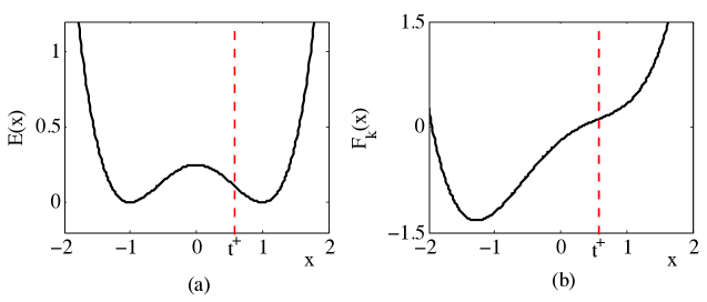
Figure 1. (a) Double-well energy defined in (16). (b) The auxiliary functional $F_{k}(x)$ with $x_{k}=t^{+}_{h}$; cf. §3.3. The second turning point $t^{-}_{h}=-t^{+}_{h}$ is an admissible descent step for $F_{k}$, hence the dimer method can potentially cycle.

It is easy to see that $x_{*}=0$ is an index-1 saddle (i.e., a maximum), and that there are two turning points $t^{\pm}=\pm 3^{-1/2}$. Thus, there exist “discrete turning points” $t^{\pm}_{h}=\pm 3^{-1/2}+O(h^{2})$ such that $\lambda(t^{\pm}_{h})=0$, where $\lambda(x)=H_{h}(x;1)\cdot 1={\textstyle\frac{1}{2h^{2}}}(E^{\prime}(x+h)-E^{\prime}(x-h))$.

Suppose that we have an iterate $x_{k}=t^{+}_{h}$, then the translation search direction is $p^{+}=\nabla_{x}\mathcal{E}_{h}(t^{+}_{h},1)<0$. Since $\mathcal{E}_{h}(t^{-}_{h})=\mathcal{E}_{h}(t^{+}_{h})$ it follows that

$$F_{k}(t^{-}_{h})=\mathcal{E}_{h}(t^{-}_{h})-2p^{+}(t^{-}_{h}-t^{+}_{h})<\mathcal{E}_{h}(t^{-}_{h})=F_{k}(t^{+}_{h}).$$

Thus, for $\Theta$ sufficiently small, the update $x_{k+1}=t^{-}_{h}$ satisfies all the conditions for termination of the loop (11)–(12) in Algorithm 3. See also Figure 1 (b), where $F_{k}$ is visualised.

We therefore conclude that our newly proposed variant of the dimer algorithm does not excluded cycling behaviour. We also remark that the example is not exclusively one-dimensional, but that analogous constructions can be readily made in any dimension.

3.4. Local convergence

We now establish a local convergence rate.

Theorem 7. Let $(x_{*},v_{*},\lambda_{*})$ be an index-1 saddle, let $(x_{h},v_{h},\lambda_{h})$ denote the dimer saddle associated with $(x_{*},v_{*},\lambda_{*})$ (cf. Theorem 2.3) and let $x_{k},v_{k}$ be the iterates generated by the Linesearch Dimer Algorithm. Then there exist $r,h_{0},C>0$ and $\gamma\in(0,1)$ such that, for $x_{0}\in B_{r}(x_{*})$, $v_{-1}\in B_{r}(v_{*})\cap S_{X}$ and $h\leq h_{0}$, one of the following alternatives are true:

• If $\nabla_{x}\mathcal{E}_{h}(x_{k},v_{k-1})=0$ for some $k\in\mathbb{N}$, then $\|x_{k}-x_{h}\|\leq Ch^{2}$.

• If $\nabla_{x}\mathcal{E}_{h}(x_{k},v_{k-1})\neq 0$ for all $k\in\mathbb{N}$, then

  $$\|x_{k}-x_{h}\|+\|v_{k}-v_{h}\|\leq C\gamma^{k}\big{(}\|x_{0}-x_{h}\|+h^{2}\|v_{-1}-v_{h}\|\big{)},$$ (17)

Sketch of proof.

Case (i) merely serves to exclude an unlikely situation, in which the Rotation algorithm is ill-defined. We do not discuss this case here, but treat it in §A.5.1. In the following assume Case (ii).

Let $r_{k}=\|x_{k}-x_{h}\|$ and $s_{k}:=\|v_{k}-v_{h}\|$.

0. We recall basic contraction results for Armijo-based linesearch methods both in a general Hilbert space and for iterates constrained to lie on the unit sphere in §A.4.

1. As a first proper step we establish that, under the termination criterion $\|(1-v_{k}\otimes v_{k})H_{h}(x_{k};v_{k})\|\leq\|\nabla_{x}\mathcal{E}_{h}(x_{k},v_{k-1})\|$ for the rotation step, it follows that $\|v_{k}-v_{h}\|\lesssim r_{k}+h^{2}s_{k-1}$. This is proven in Lemma A.5 and Lemma A.5.

2. Next, we use this result to establish that there exists a local minimizer $y_{k}$ of $F_{k}$ satisfying $\|y_{k}-x_{h}\|\lesssim r_{k}^{2}+h^{2}r_{k}+h^{4}s_{k-1}$. This is established in Lemma A.5.

3. The linesearch procedure and the upper bound on the step length ensure that the step of $x_{k}$ to $x_{k+1}$ contracts towards $y_{k}$, that is, $\|x_{k+1}-y_{k}\|_{*}\leq\gamma_{*}\|x_{k}-y_{k}\|_{*}$ for some $\gamma_{*}\in(0,1)$ and $\|\cdot\|_{*}$ the energy norm induced by $(I-2v_{*}\otimes v_{*})\nabla^{2}E(x_{*})\approx\nabla^{2}F_{k}(y_{k})$. This is obtained in Lemma A.5.

4. The three preceding steps can then be combined to establish that, for $r_{0},s_{-1},h$ sufficiently small, there exists a constant $\gamma_{3}\in(\gamma_{*},1)$ such that

$$r_{k+1}^{*}+h^{2}s_{k}\leq\gamma_{3}(r_{k}^{*}+h^{2}s_{k-1}),$$

where $r_{k}^{*}:=\|x_{k}-x_{h}\|_{*}$. This contraction result readily implies the result of the theorem.

The complete proof is given in §A.5. ∎

4. Numerical Tests

4.1. Remarks on the implementation

Here, we remark on how preconditioning is implemented and on some further details of our implementation that slightly deviate from the theoretical formulations of Algorithms 1 and 3.

In all cases the underlying space is $X=\mathbb{R}^{N}$ for some $N\in\mathbb{N}$. The main deviation from Algorithms 1 and 3 is that we admit general Euclidean norms and inner products that may change from one step to another,

$$\|u\|=\sqrt{u^{T}M_{k}u},\qquad\text{and}\qquad u\cdot v=u^{T}M_{k}v,$$

where $M_{k}$ is symmetric and positive definite. That is, our implementation is a variable metric variant.

Let $E\in C^{4}(X)=C^{4}(\mathbb{R}^{N})$, and let $\nabla^{\prime}$ denote the standard gradient and $\otimes^{\prime}$ the standard tensor product (i.e., the gradient and tensor products with respect to the $\ell^{2}$-norm), then the gradient and tensor products in step $k$ become

$$\nabla E(x)=M_{k}^{-1}\nabla^{\prime}E(x),\quad\text{and}\quad(v\otimes v)\nabla E(x)=(v\otimes^{\prime}v)\nabla^{\prime}E(x).$$

The variable metric variant of Algorithm 1, augmented with a termination criterion, is given below. For the purposes of the numerical testing we call this the simple dimer method, it is effectively a forward Euler ODE integrator for the dimer dynamics. (Note also that here the rotation step is performed by a simple descent step followed by a projection, rather than a step on the manifold.)

Algorithm 1${}^{\mbox{\tiny vm}}$:

1. Input: $x_{0},v_{0}\in X$, $h>0$,$\alpha,\beta>0$,${\rm TOL}^{x},{\rm TOL}^{v}>0$; $k:=0$;

2. While $\|M_{k}^{-1/2}\nabla_{x}^{\prime}\mathcal{E}_{h}(x_{k},v_{k})\|_{\ell^{2}}>{\rm TOL}^{x}$
   .                    or $\|(M_{k}^{-1/2}-M_{k}^{1/2}v_{k}\otimes^{\prime}v_{k})h^{-2}\nabla_{v}^{\prime}\mathcal{E}_{h}(x_{k},v_{k})\|_{\ell^{2}}>{\rm TOL}^{v}$    do

3. %% Metric %%

4. Compute a spd matrix $M_{k}\in\mathbb{R}^{N\times N}$;

5. $v_{k}:=v_{k}/\|M_{k}^{1/2}v_{k}\|$;

6. $v_{k+1}:=v_{k}-\beta(M_{k}^{-1}-v_{k}\otimes v_{k})h^{-2}\nabla_{v}^{\prime}\mathcal{E}_{h}(x_{k},v_{k})$

7. $x_{k+1}:=x_{k}-\alpha(M_{k}^{-1}-2v_{k}\otimes v_{k})\nabla_{x}^{\prime}\mathcal{E}_{h}(x_{k},v_{k})$.

8. $k:=k+1$

Remark 8. In our experiments we observe that the rotation residual decreases more quickly than the translation residual, hence the convergence criteria could be based on the translation residual only, without affecting the results. ∎

Remark 9. Our analysis of both the Simple Dimer Algorithm and of the Linesearch Dimer Algorithm is readily extended to their variable metric variants, provided that the metric $M_{k}$ at iterate $k$ is a smooth function of the state, i.e., $M_{k}={\bf M}(x_{k},v_{k})$, where ${\bf M}\in C^{2}(B_{r}(x_{*})\times S_{X};L(X))$, for some $r>0$. This is the case in all examples that we consider below. A more general convergence theory, e.g., employing quasi-Newton type hessian updates requires additional work. ∎

Analogous modifications are made to Algorithm 3. The auxiliary functional $F_{k}$ now reads

$$F_{k}(x) =\mathcal{E}_{h}(x;v_{k})-2\big{(}v_{k}^{T}\nabla_{x}^{\prime}\mathcal{E}_{h}(x_{k},v_{k})\big{)}\big{(}v_{k}^{T}M_{k}(x-x_{k})\big{)}+\lambda_{k}\big{(}v_{k}^{T}M_{k}(x-x_{k})\big{)}^{2},$$

$$\lambda_{k} =h^{-2}v_{k}^{T}\nabla_{v}^{\prime}\mathcal{E}_{h}(x_{k},v_{k}),$$

$$\nabla_{x}^{\prime}\mathcal{E}_{h}(x,v) ={\textstyle\frac{1}{2}}\big{(}\nabla^{\prime}E(x+hv)+\nabla^{\prime}E(x-hv)\big{)},$$

$$\nabla_{v}^{\prime}\mathcal{E}_{h}(x,v) ={\textstyle\frac{h}{2}}\big{(}\nabla^{\prime}E(x+hv)-\nabla^{\prime}E(x-hv)\big{)},$$

where we recall that $\nabla^{\prime}$ denotes the standard gradient (i.e., the gradient with respect to the $\ell^{2}$-norm).

Algorithm 3${}^{\mbox{\tiny vm}}$:

1. Input: $x_{0},v_{0}\in X$, $h>0$,${\rm TOL}^{x},{\rm TOL}^{v}>0$; $k:=0$;

2. While $\|M_{k}^{-1/2}\nabla_{x}^{\prime}\mathcal{E}_{h}(x_{k},v_{k})\|_{\ell^{2}}>{\rm TOL}^{x}$

3. %% Metric %%

4. Compute a spd matrix $M_{k}\in\mathbb{R}^{N\times N}$;

5. $v_{k}^{\prime}:=v_{k}/\|M_{k}^{1/2}v_{k-1}\|$;

6. %% Rotation %%

7. $v_{k+1}:=\text{\bf Rotation (VM)}[x_{k},v_{k}^{\prime},\beta,M_{k}]$

8. %% Translation %%

9. $p_{M}:=-(M_{k}^{-1}-2v_{k+1}\otimes v_{k+1})\nabla_{x}^{\prime}\mathcal{E}_{h}(x_{k};v_{k+1})$

10. $\alpha:=\min(\alpha_{\rm max},2\alpha)$

11. While ($F_{k}(x_{k}+\alpha p_{M})>F_{k}(x_{k})-\Theta\alpha p_{M}^{T}M_{k}p_{M}$)
    .             or ($\|M_{k}^{1/2}(M_{k}^{-1}-v_{k+1}\otimes v_{k+1})h^{-2}\nabla_{v}^{\prime}\mathcal{E}_{h}(x_{k}+\alpha p_{M};v_{k+1})\|_{\ell^{2}}>$
    .                   $\Psi\|M_{k}^{1/2}(M_{k}^{-1}-v_{k+1}\otimes v_{k+1})h^{-2}\nabla_{v}^{\prime}\mathcal{E}_{h}(x_{k};v_{k+1})\|_{\ell^{2}}$) do

12. $\alpha:=\alpha/2$

13. $x_{k+1}:=x_{k}+\alpha p_{M}$.

14. $k:=k+1$

Rotation${}^{\mbox{\tiny vm}}$:

1. Input: $x,v,\beta,M_{k}$
   Parameters: ${\rm TOL}=\max(\|M_{k}^{-1/2}\nabla_{x}^{\prime}\mathcal{E}_{h}(x,v)\|_{\ell^{2}},{\rm TOL}^{v}$), $\Theta\in(0,1)$, $\beta_{\rm max}$;

2. While $\|M_{k}^{1/2}(M_{k}^{-1}-v\otimes v)h^{-2}\nabla_{v}^{\prime}\mathcal{E}_{h}(x;v)\|>{\rm TOL}$ do

3. $s:=-(M_{k}^{-1}-v\otimes v)h^{-2}\nabla_{v}^{\prime}\mathcal{E}_{h}(x;v)$

4. $t:=\|M_{k}^{1/2}s\|_{\ell^{2}}$; $\beta:=\min(\beta_{\rm max},2\beta)$

5. $v_{\beta}:=\cos(t\beta)v+\sin(t\beta)t^{-1}s$

6. While $\mathcal{E}_{h}(x,v_{\beta})>\mathcal{E}_{h}(x,v)-\Theta\beta t^{2}$ do

7. $\beta:=\beta/2$

8. $v:=v_{\beta}$

9. Output: $v,\beta$

Remark 10. An additional (optional) modification that can give significant performance gains is to employ a different heuristic for the initial guess of $\alpha$ in Step (7) of Algorithm 3${}^{\mbox{\tiny vm}}$: With $p_{M,k}:=-(M_{k}^{-1}-2v_{k}\otimes v_{k})\nabla_{x}^{\prime}\mathcal{E}_{h}(x_{k};v_{k})$ and $p_{I,k}:=-(I-2v_{k}\otimes v_{k})\nabla_{x}^{\prime}\mathcal{E}_{h}(x_{k},v_{k})$ let, for $k\geq 2$, $\gamma_{k}:=(p_{M,k-1}\cdot^{\prime}p_{I,k-1})/(p_{M,k}\cdot^{\prime}p_{I,k})$, then for $k\geq 2$ we replace Step (7) with

$$\alpha:=\min\big{(}\mathrm{avg}(\gamma_{\max(2,k-4)},\ldots,\gamma_{k}),2\alpha,\alpha_{\rm max})$$

An analogous modification can be made for the rotation algorithm. ∎

In all numerical tests we use the following parameters: $h=10^{-3}$, $\Theta=\sqrt{0.1}$, ${\rm TOL}^{x}=10^{-5}$, ${\rm TOL}^{v}=10^{-1}$, $\alpha_{\rm max}=1$ and $\Psi=100$. We briefly discuss these choices:

• $h$ should be small enough such that the dimer saddle is sufficiently close to the true saddle (with respect to the length scales of the given problem), while large enough that numerical robustness does not become a problem for the rotation. In all our tests, $h=10^{-3}$ was a good compromise.

• $\Theta$ should be sufficiently large (though, $\leq 1/2$) to ensure that the linesearch method finds steps which give a large decrease in dimer energy. It is often chosen much smaller than our choice of $\Theta=\sqrt{0.1}$ to immediately accept steps that make some progress. Our experience is that, with preconditioned search direction, our more stringent choice gives better performance.

• The choice of ${\rm TOL}^{x}$ simply controls the desired level of convergence to the dimer saddle.

• The parameter ${\rm TOL}^{v}$ should be chosen as weakly as possible such that either algorithm converges to the saddle. In Algorithm 3${}^{\mbox{\tiny vm}}$ rotations are performed such that the rotation residual is at least as good as the translation residual until it moves below this value. Subsequent translations may increase the rotation residual such that further applications of the rotation algorithm are needed. In practise this means that the rotation algorithm is performed at every iteration of Algorithm 3’ for the first few steps, then only sporadically or not at all once the rotation residual reaches ${\rm TOL}^{v}$. The use of this parameter then decreases the overall number of gradient evaluations needed to find the dimer saddle, by only performing the rotation as necessary.

• The maximum step $\alpha_{\rm max}$ should principally be chosen such that the dimer cannot translate into non-physical regimes for the given problem.

• The parameter $\Psi$ should be chosen $>1$ and restricts the translation step from moving the dimer to a point where it becomes too badly orientated. In our numerical tests this parameter is set sufficiently large that this termination criteria for the translation never occurs (the translation always terminates by finding a sufficient decrease in the auxiliary functional $F_{k}$).

Remark 11. We observe during numerical testing that the rotation component of the linesearch dimer is somewhat vulnerable to rounding error in the objective function $E$. As the dimer becomes increasingly well orientated, $\nabla E$ becomes almost orthogonal to the dimer orientation and any small rotation may result in a zero change (to numerical precision) in the dimer energy. In the numerical examples presented in this section, this never occurs since we use a relatively high value for ${\rm TOL}^{v}$, that is the rotation is only ever weakly converged. In our examples this is sufficient for the the dimer to converge to the saddle. If a stronger level of converge were required, another technique should be used to improve the rotation residual further, such as changing to a gradient based method or simply making fixed steps. ∎

4.2. Test 1: A simple 2D example

Our first example is taken from [28]. We equip $X=\mathbb{R}^{2}$ with the standard Euclidean inner product. The energy function is given by $E(x,y)=(x^{2}-1)^{2}+y^{2}$, which has two simple symmetric minima at $(\pm 1,0)$ and a unique index-1 saddle at $(0,0)$. The energy function is given graphically in Figure 2.

Figure 3 shows the $x$-residual $\|\nabla_{x}\mathcal{E}_{h}(x,v)\|$ plotted against the number of function evaluations and the number of iterations.

The performance of the linesearch dimer is compared with a simple dimer method with different step sizes. Evidently a good choice of step is important. If a poor choice is made the algorithm may perform poorly or diverge. The linesearch dimer method requires a certain amount of overhead versus a simple dimer with well chosen step sizes. We can see in Figure 3 that the linesearch dimer may find a solution in fewer dimer iterations than the best fixed step tested (indicating that it found better steps), but using more gradient evaluations.

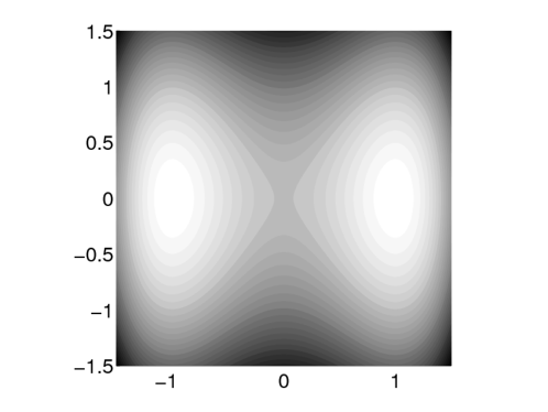
Figure 2. Energy function for Test 1 with 2 symmetric minima and a unique index-1 saddle

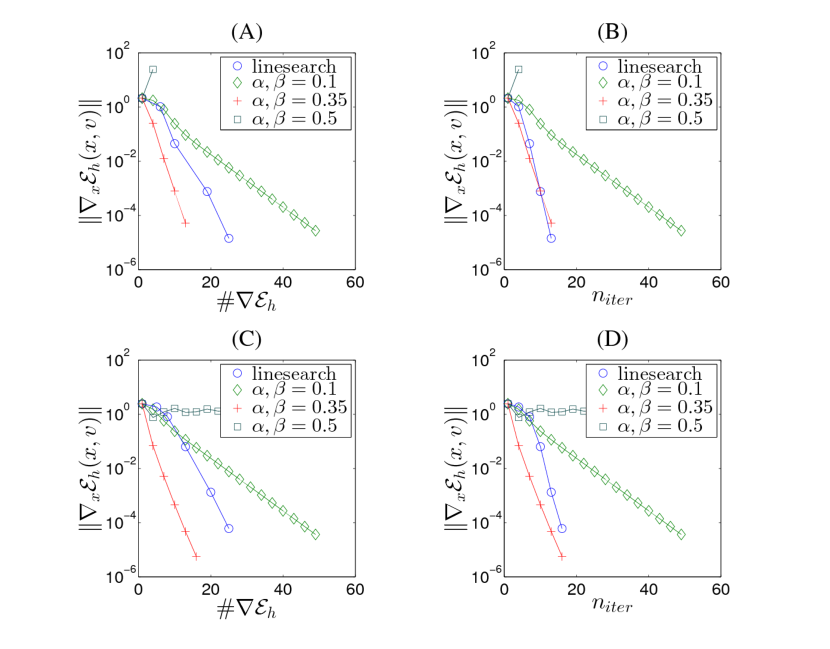
Figure 3. Convergence of the dimer to the saddle in a simple 2D example (Test 1).(A,B) The $\ell_{2}$ norm of the $x$ gradient versus the number of force evaluations and the number of dimer iteration where the initial dimer state is $x=[0.2,1],v=[1,1]$. In this case the choice $\alpha,\beta=0.5$ diverges immediately. (C,D) The $\ell_{2}$ norm of the $x$ gradient versus the number of force evaluations and the number of dimer iterations where the initial dimer state is $x=[0.2,1],v=[1,1]$.

4.3. Test 2: Vacancy Diffusion

Our second test case is a standard example from molecular physics. A single atom is removed from a 2D lattice and a neighbouring atom is moved partway into the gap. Atoms within a certain radius of the vacancy are allowed to move, while those beyond that radius are fixed. This configuration is illustrated in Figure 4(A).

The energy function is given by the simple Morse potential,

$$E(\{x_{i}\})=\sum_{i,j}V(\|x_{i}-x_{j}\|_{2}),\qquad V(r)=e^{-2a(r-1)}-2e^{-a(r-1)},$$ (18)

with stiffness parameter $a=4$.

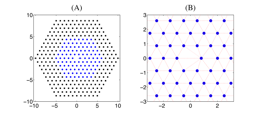
Figure 4. Initial configuration of the atoms in the vacancy diffusion problem (Test 2) . Black squares are fixed atoms while blue circles are atoms which move freely. (A) The initial dimer orientation is selected so that the translated atom has an orientation along the $y=0$ direction, and is zero for all other atoms. (B) The Delaunay $\mathcal{T}_{k}$ triangulation used for the connectivity norm.

This test case demonstrates the importance of selecting the correct norm for high-dimensional problems. The experiment is run both using the generic $\ell_{2}$ norm (no preconditioner), as well as a ‘connectivity’ norm. Such a norm can be defined based on the Delaunay triangulation of the atomistic positions (Figure 4(B))

$$\langle M_{k}u,u\rangle=\int|\nabla I_{\mathcal{T}_{k}}u|^{2},$$

where $\mathcal{T}_{k}$ is the triangulation depicted in the figure and $I_{\mathcal{T}_{k}}$ the associated nodal interpolant.

Figure 5 demonstrates the convergence to the saddle with different numbers of free atoms $nA$ (giving different dimensionality of the system) in the two norms for the linesearch dimer.

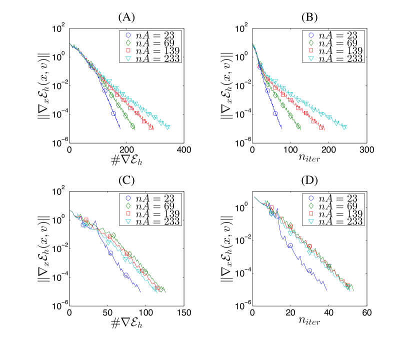
Figure 5. Convergence of the linesearch dimer to the saddle in the vacancy diffusion problem (Test 2) with (A),(C) the $\ell_{2}$ norm and (B),(D) connectivity norm versus the number of force evaluations and dimer iterations for increasing numbers of free atoms.

We can also observe the benefit of the linesearch vs a simple dimer scheme when using the connectivity norm (Figure 6). The linesearch dimer selects very efficient stepsizes with no a-priori information, while the simple dimer method might exhibit either slow convergence, or no convergence, if the fixed steps are poorly chosen.

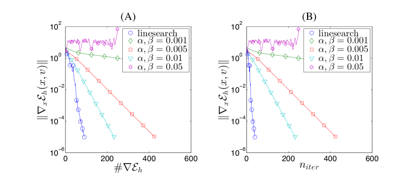
Figure 6. Convergence of the linesearch dimer vs the simple dimer method for Test 2 some choice of the of simple dimer step sizes with $nA=69$ using the connectivity norm.

4.4. Test 3: A Phase Field Example

Our final example is based on a simple phase field model where the global energy is given by,

$$E(u)=\int_{\Omega}\frac{\epsilon}{2}\left|\nabla u\right|^{2}+\frac{1}{2\epsilon}(u^{2}-1)^{2}.$$ (19)

In our test $\Omega$ is the unit square, and the boundary conditions are,

$$u(x)=\left\{\begin{array}[]{rl}-1,&x_{1}\in\{0,1\}\\ 1,&x_{2}\in\{0,1\}.\end{array}\right.$$ (20)

There are 2 minima of such an energy, these are given in Figure 7(A),(B). The saddle between these two minima is given in Figure 7(C).

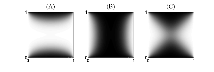
Figure 7. Minima (A,B) and saddle point (C) of the phase field problem (Test 3) with $\epsilon=1/10$. The shading is linearly interpolated between white(-1) and black(1).

A possible choice for a preconditioner for this system is a stabilized Laplacian,

$$P=\epsilon\Delta+\frac{1}{\epsilon}I.$$ (21)

In order to compute either a minimum or a saddle point for such a system we triangulate the domain into a variable number of elements, thereby creating a discrete system of variable dimensionality. In our tests we take the initial dimer point as a small random perturbation of one of the local minima, and the initial dimer orientation is the metric inverted against a vector of ones.

In Figure 8 we demonstrate the necessity of using a preconditioner to solve this problem using the simple dimer method. When using the preconditioner (21), the algorithm performs well when the step size is chosen appropriately. We observe the expected behaviour, that there exists an optimal step size where convergence is fastest, and beyond that step size the dimer diverges. In fact we observe that the stabilized Laplacian metric is so effective, that the optimal step size seems very close to the unit step. If the $\ell_{2}$ norm (identity preconditioner) is used then for all step sizes tested the dimer diverges, indicating that at best a very small step would need to be chosen for convergence.

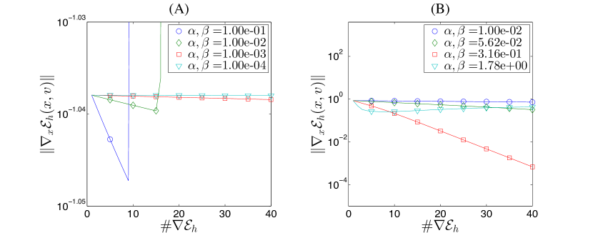
Figure 8. Convergence of the simple dimer to the saddle in the phase field problem (Test 3) with (A) the $\ell_{2}$ metric and (B) the stabilized Laplacian metric where $\epsilon=1/10$ for a triangulation with 3485 degrees of freedom.

In Figure 9 we demonstrate that the used of the scaled Laplacian metric for different system sizes. We observe that the use of this metric gives almost perfect scale invariance.

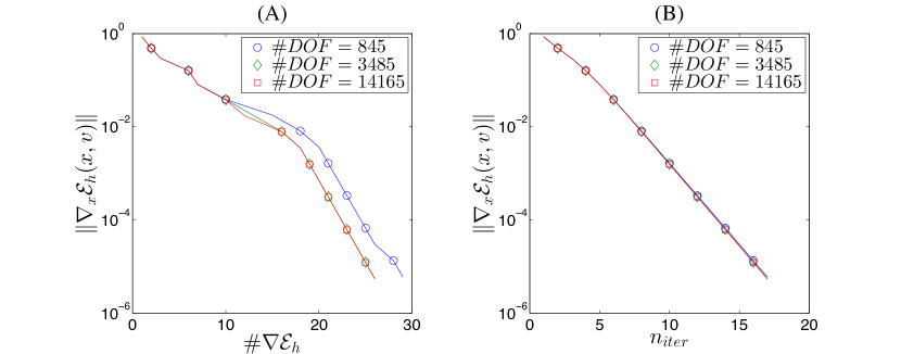
Figure 9. Convergence of the linesearch dimer to the saddle in the phase field problem (Test 3) with the stabilized Laplacian metric and triangulations of varying coarseness.

In Figure 10 we give the results of applying the simple and linesearch dimers with varying $\epsilon$; the coarseness of the discretization in each experiment is chosen such that $\Delta x\approx\epsilon/5$. In some of these cases the linesearch dimer fails due to rounding error. Specifically, due to rounding error in the naive implementation of the energy function (simple summation over the elements), the translation step fails to find a sufficient decrease in the dimer energy, the step size selected shrinks to zero (to rounding error) and the method stagnates. In order to correct this a more robust method of evaluating the energy or a more advanced optimization algorithm should be implemented which can either choose better linesearch directions or more robustly deal with numerically zero energy changes.

We also observe, in the case $\epsilon=1/30$ that the rate of convergence of even the simple dimer changes once the residual moves below a certain value. We are unable to give a satisfactory explanation for this effect, but speculate that the singularity in the boundary condition (which excludes admissible $H^{1}$-states) might be the case. (In particular, we observed that this behaviour is independent of the mesh coarseness and of the dimer length.)

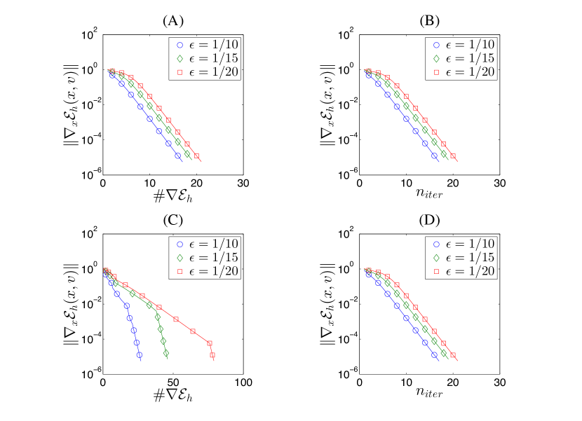
Figure 10. Convergence to the saddle in the phase field problem (Test 3) using the stabilized Laplacian metric with (A),(B) the simple dimer with unit step length and (C),(D) the linesearch dimer for a triangulation with 2405,9805,22205 degrees of freedom for the respective choices of $\epsilon$.

5. Conclusions

We have described a dimer method for finding a saddle point in which the dimer length $h$ is not required to shrink to zero, but which converges to a point that lies within $O(h^{2})$ of a saddle. We have enhanced this algorithm with a lineasearch to improve its robustness, and use the observation that the dimer method may be formulated and applied in a general Hilbert space to allow preconditioning that improves the method’s efficiency. The linesearch uses a local merit function. Unfortunately our particular merit function may not lead to global convergence of the iterates, and it is an open question as to whether there is another merit function that ensures global convergence. We have illustrated the positive effects of our algorithms on three realistic examples.

Appendix A Proofs

A.1. Proof of Proposition 2.3

We prove the result using the inverse function theorem. We write (9) as $F(x_{h},v_{h},\lambda_{h})=0$ and show that $\|F(x_{*},v_{*},\lambda_{*})\|\leq Ch^{2}$ and that $\nabla F(x_{*},v_{*},\lambda_{*})$ is an isomorphism with bounds independent of $h$. The inverse function theorem then yields the stated result.

Residual estimate. Let the residual components be

$$r_{x} :=F_{x}(x_{*},v_{*},\lambda_{*})={\textstyle\frac{1}{2}}\big{(}\nabla E(x_{*}+hv_{*})+\nabla E(x_{*}-hv_{*})\big{)},$$

$$r_{v} :=F_{v}(x_{*},v_{*},\lambda_{*})={\textstyle\frac{1}{2h}}(\nabla E(x_{*}+hv_{*})-\nabla E(x_{*}-hv_{*}))-\lambda_{*}v_{*},$$

$$r_{\lambda} :=F_{\lambda}(x_{*},v_{*},\lambda_{*})={\textstyle\frac{1}{2}}(\|v_{*}\|^{2}-1).$$

Then,

$$r_{x} =\nabla E(x_{*})+{\textstyle\frac{1}{2}}\nabla^{2}E(x_{*})(hv_{*}-hv_{*})+O(h^{2})=O(h^{2}),$$

$$r_{v} =\nabla^{2}E(x_{*})v_{*}-\lambda_{*}v_{*}+{\textstyle\frac{1}{h}}\big{(}\nabla^{3}E(x_{*})[hv_{*}\otimes hv_{*}-hv_{*}\otimes hv_{*}]+O(h^{2})=O(h^{2}),$$

$$r_{\lambda} =0.$$

Thus, $\|F(x_{*},v_{*},\lambda_{*})\|\leq Ch^{2}$.

Stability. $\nabla F(x_{*},v_{*},\lambda_{*})$ can be written in the form

$$\nabla F(x_{*},v_{*},\lambda_{*}) =\left[\begin{matrix}\frac{\nabla^{2}E(x_{*}+hv_{*})+\nabla^{2}E(x_{*}-hv_{*})}{2}&h\frac{\nabla^{2}E(x_{*}+hv_{*})-\nabla^{2}E(x_{*}-hv_{*})}{2}&0\\ \frac{\nabla^{2}E(x_{*}+hv_{*})-\nabla^{2}E(x_{*}-hv_{*})}{2h}&\frac{\nabla^{2}E(x_{*}+hv_{*})+\nabla^{2}E(x_{*}-hv_{*})}{2}-\lambda_{*}I&v_{*}\\ 0&v_{*}^{T}&0\end{matrix}\right]$$

$$=\left[\begin{matrix}\nabla^{2}E(x_{*})&0&0\\ \nabla^{3}E(x_{*})\cdot v_{*}&\nabla^{2}E(x_{*})-\lambda_{*}I&v_{*}\\ 0&v_{*}^{T}&0\end{matrix}\right]+O(h^{2})=:{\bf A}+O(h^{2}).$$

where we used (3), (4) and (6). By assumption, $\nabla^{2}E(x_{*})$ is an isomorphism on $X$. Since, also by assumption, $\lambda_{*}$ is a simple eigenvalue, the block

$$\left[\begin{matrix}\nabla^{2}E(x_{*})-\lambda_{*}I&v_{*}\\ v_{*}^{T}&0\end{matrix}\right]$$ (22)

is an isomorphism on $X\times\mathbb{R}$ as well. Thus, ${\bf A}$ is an isomorphism on $X\times X\times\mathbb{R}$ and consequently, for all $h$ sufficiently small, $\nabla F(x_{*},v_{*},\lambda_{*})=A+O(h^{2})$ is also an isomorphism, with a uniform bound on its inverse.

Thus, the inverse function theorem shows that there exist a radius $r_{0}>0$ and a dimer length $h_{0}>0$, such that, for $h\leq h_{0}$, there exists a unique solution $(x_{h},v_{h},\lambda_{h})$ to (9) in a ball of radius $r_{0}$ about $(x_{*},v_{*},\lambda_{*})$, satisfying the estimate (10).

A.2. Proof of Theorem 2.4 (a)

Fix $r$ and $h_{0}$ sufficiently small so that Theorem 2.3 applies. Let $e_{k}:=x_{k}-x_{h},f_{k}:=v_{k}-v_{h}$ and $r_{k}:=\sqrt{\|e_{k}\|^{2}+\|f_{k}\|^{2}}$, so that trivially $\|e_{k}\|\leq r_{k}$ and $\|f_{k}\|\leq r_{k}$.

Lemma 12. Let $p:=-(I-2v_{k}\otimes v_{k})\nabla_{x}\mathcal{E}(x_{k},v_{k})$ and $s:=-(I-v_{k}\otimes v_{k})H_{h}(x_{k};v_{k})$, then, under the assumptions of Theorem 2.4,

$$p =-Ae_{k}+O(r_{k}^{2}+h^{2}r_{k}),\qquad\text{and}$$ (23)

$$s =-Be_{k}-Cf_{k}+O(r_{k}^{2}+h^{2}r_{k}),$$ (24)

where the operators $A$ and $C$ are defined in (14) and $B$ is a bounded linear operator.

Proof.

To prove (23) we first note the following identities which are easy to establish:

$$\nabla_{x}\mathcal{E}_{h}(x,v) =\nabla E(x)+O(h^{2}),$$

$$\nabla_{x}\mathcal{E}_{h}(x_{k},v_{k})-\nabla_{x}\mathcal{E}_{h}(x_{h},v_{h}) =O(r_{k}),$$

$$v_{k}\otimes v_{k}-v_{h}\otimes v_{h} =O(r_{k}),$$

$$\nabla_{x}^{2}\mathcal{E}_{h}(x_{h},v_{h}) =\nabla^{2}E(x_{h})+O(h^{2})=\nabla^{2}E(x_{*})+O(h^{2})$$

$$\nabla_{x}\nabla_{v}\mathcal{E}_{h}(x_{h},v_{h}) ={\textstyle\frac{1}{2}}\big{(}\nabla^{2}E(x_{h}+hv_{h})-\nabla^{2}E(x_{h}-hv_{h})\big{)}=O(h^{2}).$$ (25)

Using these identities, we can expand

$$p =-(I-2v_{k}\otimes v_{k})\big{(}\nabla_{x}\mathcal{E}_{h}(x_{k},v_{k})-\nabla_{x}\mathcal{E}_{h}(x_{h},v_{h})\big{)},$$

$$=-(I-2v_{h}\otimes v_{h})\big{(}\nabla_{x}^{2}\mathcal{E}_{h}(x_{h},v_{h})e_{k}+\nabla_{x}\nabla_{v}\mathcal{E}_{h}(x_{h},v_{h})f_{k}\big{)}+O(r_{k}^{2})$$

$$=-(I-2v_{h}\otimes v_{h})\nabla^{2}E(x_{h})e_{k}+O(r_{k}^{2}+h^{2}r_{k})$$

$$=-(I-2v_{*}\otimes v_{*})\nabla^{2}E(x_{*})e_{k}+O(r_{k}^{2}+h^{2}r_{k})$$

$$=-Ae_{k}+O(r_{k}^{2}+h^{2}r_{k}).$$

To prove (24), we first note that, with $\|v\|=1$,

$$H_{h}(x;v) =\mathchoice{{\vbox{\hbox{$\textstyle-$ }}\kern-7.83337pt}}{{\vbox{\hbox{$\scriptstyle-$ }}\kern-5.90005pt}}{{\vbox{\hbox{$\scriptscriptstyle-$ }}\kern-4.75003pt}}{{\vbox{\hbox{$\scriptscriptstyle-$ }}\kern-4.25003pt}}\!\int_{-1}^{1}\nabla^{2}E(x+thv)\,{\rm d}t\,v=\nabla^{2}E(x)v+O(h^{2}),$$

$$H_{h}(x_{h};v_{h}) =\nabla^{2}E(x_{h})v_{h}+O(h^{2})=\nabla^{2}E(x_{*})v_{*}+O(h^{2}),$$

$$H_{h}(x_{k};v_{k})-H_{h}(x_{h};v_{h}) =\mathchoice{{\vbox{\hbox{$\textstyle-$ }}\kern-7.83337pt}}{{\vbox{\hbox{$\scriptstyle-$ }}\kern-5.90005pt}}{{\vbox{\hbox{$\scriptscriptstyle-$ }}\kern-4.75003pt}}{{\vbox{\hbox{$\scriptscriptstyle-$ }}\kern-4.25003pt}}\!\int_{-1}^{1}\Big{(}\nabla^{2}E(x_{k}+thv_{k})-\nabla^{2}E(x_{h}+thv_{h})\Big{)}\,{\rm d}t\,v_{k}$$

$$\qquad\qquad+\mathchoice{{\vbox{\hbox{$\textstyle-$ }}\kern-7.83337pt}}{{\vbox{\hbox{$\scriptstyle-$ }}\kern-5.90005pt}}{{\vbox{\hbox{$\scriptscriptstyle-$ }}\kern-4.75003pt}}{{\vbox{\hbox{$\scriptscriptstyle-$ }}\kern-4.25003pt}}\!\int_{-1}^{1}\nabla^{2}E(x_{h}+thv_{h})\,{\rm d}t(v_{k}-v_{h})$$

$$=\mathchoice{{\vbox{\hbox{$\textstyle-$ }}\kern-7.83337pt}}{{\vbox{\hbox{$\scriptstyle-$ }}\kern-5.90005pt}}{{\vbox{\hbox{$\scriptscriptstyle-$ }}\kern-4.75003pt}}{{\vbox{\hbox{$\scriptscriptstyle-$ }}\kern-4.25003pt}}\!\int_{-1}^{1}\Big{(}\nabla^{3}E(x_{h}+thv_{h})\big{[}(x_{k}-x_{h})+th(v_{k}-v_{h})\big{]}\,{\rm d}tv_{h}$$

$$\qquad\qquad+\nabla^{2}E(x_{*})(v_{k}-v_{h})+O(r_{k}^{2}+h^{2}r_{k})$$

$$=(\nabla^{3}E(x_{*})v_{*})e_{k}+\nabla^{2}E(x_{*})f_{k}+O(h^{2}r_{k}+r_{k}^{2}),$$

where we interpret $\nabla^{3}E(x)\cdot v\in L(X)$ via the action $w\cdot((\nabla^{3}E(x)\cdot v)z)=\lim_{t\to 0}t^{-1}w\cdot((\nabla^{2}E(x+tv)-\nabla^{2}E(x))z)$. Finally, we also have

$$(v_{k}\otimes v_{k}-v_{h}\otimes v_{h})H_{h}(x_{h};v_{h}) =(v_{k}\otimes v_{k}-v_{h}\otimes v_{h})\nabla^{2}E(x_{*})v_{*}+O(h^{2}r_{k})$$

$$=\lambda_{*}(v_{k}\otimes v_{k}-v_{h}\otimes v_{h})v_{*}+O(h^{2}r_{k})$$

$$=\lambda_{*}(v_{k}\otimes v_{k}-v_{h}\otimes v_{h})v_{h}+O(h^{2}r_{k})$$

$$=\lambda_{*}(v_{k}-v_{h})+\lambda_{*}v_{k}((v_{k}-v_{h})\cdot v_{h})+O(h^{2}r_{k})$$

$$=\lambda_{*}f_{k}+O(r_{k}^{2}+h^{2}r_{k}).$$

In the very last line we also used the fact that $v_{k}\cdot v_{h}-1={\textstyle\frac{1}{2}}\|v_{k}-v_{h}\|^{2}$.

Using these identities, we can compute

$$s =-(I-v_{k}\otimes v_{k})H_{h}(x_{k};v_{k})$$

$$=(I-v_{h}\otimes v_{h})H_{h}(x_{h};v_{h})-(I-v_{k}\otimes v_{k})H_{h}(x_{k};v_{k})$$

$$=-(I-v_{k}\otimes v_{k})\big{(}H_{h}(x_{k};v_{k})-H_{h}(x_{h};v_{h})\big{)}+(v_{k}\otimes v_{k}-v_{h}\otimes v_{h})H_{h}(x_{h};v_{h})$$

$$=-(I-v_{k}\otimes v_{k})\big{(}(\nabla^{3}E(x_{*})v_{*})e_{k}+\nabla^{2}E(x_{*})f_{k}\big{)}+O(h^{2}r_{k}+r_{k}^{2})$$

$$\qquad\qquad+\lambda_{*}f_{k}+O(r_{k}^{2}+h^{2}r_{k})$$

$$=:-Be_{k}+\big{[}\lambda_{*}I-(I-v_{*}\otimes v_{*})\nabla^{2}E(x_{*})\big{]}f_{k}+O(r_{k}^{2}+h^{2}r_{k})$$

$$=-Be_{k}-Cf_{k}+O(r_{k}^{2}+h^{2}r_{k}).\qed$$

From Lemma A.2 it follows in particular that $s=O(r_{k})$. Hence, Taylor expansions of sine and cosine in the identity

$$v_{k+1}=\cos\big{(}\|s\|\beta_{k})v_{k}+\sin(\|s\|\beta_{k}){\textstyle\frac{s}{\|s\|}},$$

yield

$$f_{k+1}=f_{k}+\beta_{k}s+O(\beta_{k}^{2}s_{k}^{2})$$

Using Lemma A.2, the identity $e_{k+1}=e_{k}+\alpha_{k}p$, and the fact that $\beta_{k}$ is bounded, we therefore obtain identity (13) in the proof outline.

Upon defining

$${\bf A}_{k}:=\left(\begin{matrix}\alpha_{k}A&0\\ \beta_{k}B&\beta_{k}C\end{matrix}\right)\quad\text{and}\quad{\bf e}_{k}=\left(\begin{matrix}e_{k}\\ f_{k}\end{matrix}\right)$$

(13) reads

$${\bf e}_{k+1}=(I-{\bf A}_{k}){\bf e}_{k}+{\bf t}_{k},$$ (26)

where

$$\|{\bf t}_{k}\|\leq C_{\rm t}(\alpha_{k}+\beta_{k})(h^{2}+r_{k})r_{k}.$$

Due to the fact that $A$ is symmetric and positive definite, it follows that, for $\bar{\alpha},\bar{\beta}$ chosen sufficiently small and $\underline{\alpha}=\inf_{k}\alpha_{k},\underline{\beta}=\inf_{k}\beta_{k}>0$, the spectrum of $I-{\bf A}_{k}$ is real and belongs to $[0,1-\epsilon]$ for some $\epsilon>0$, that depends on $\underline{\alpha},\underline{\beta}$. This will be crucial later in the proof.

Lemma 13. Let ${\bf P}_{n,k}:=\prod_{i=n}^{k}(I-{\bf A}_{i})$, for $0\leq n\leq k$, then there exist constants $C_{1}>1,\mu\in(0,1)$ such that

$$\|{\bf P}_{n,k}\|\leq C_{1}\mu^{k-n+1}.$$ (27)

Proof.

We assume, without loss of generality, that $n=0$. First, we note that the diagonal blocks

$$A_{k}:=[{\bf P}_{0,k}]_{xx}=\prod_{i=0}^{k}(I-\alpha_{k}A),\quad\text{and}\quad C_{k}:=[{\bf P}_{0,k}]_{vv}=\prod_{i=0}^{k}(I-\beta_{k}C),$$

and it is easy to see that, for $\underline{\alpha}\leq\alpha_{i}\leq\bar{\alpha},\underline{\beta}\leq\beta_{i}\leq\bar{\beta}$ chosen sufficiently small, that

$$\|A_{k}\|\leq\bar{\mu}^{k}\qquad\text{and}\qquad\|C_{k}\|\leq\bar{\mu}^{k}.$$ (28)

where $\bar{\mu}:=\max\big{(}1-\underline{\alpha}\inf\sigma(A),1-\underline{\beta}\inf\sigma(C)\big{)}\in(0,1)$.

Since the off-diagonal block $[{\bf P}_{0,k}]_{xv}=0$, it remains to estimate the off-diagonal block $B_{k}:=[{\bf P}_{0,k}]_{vx}$. We use induction over $k$. Let $C_{*}:=\bar{\mu}^{-1}\underline{\beta}\|B\|$ and suppose that

$$\|B_{k}\|\leq C_{*}k\bar{\mu}^{k}.$$ (29)

Then, using

$$B_{k+1}=-\beta_{k+1}BA_{k}+(I-\beta_{k+1}C)B_{k},$$

as well as $\|I-\beta_{k+1}C\|\leq\bar{\mu}$ we can estimate

$$\|B_{k+1}\|\leq\underline{\beta}\|B\|\bar{\mu}^{k}+\bar{\mu}C_{*}k\bar{\mu}^{k}=C_{*}(k+1)\bar{\mu}^{k+1},$$

which establishes the induction since the result is true by definition of $C_{*}$ when $k=0$.

Now pick $\tau>1$ so that $\mu:=\tau\bar{\mu}<1$. Then (28) give that $\|A_{k}\|\leq\mu^{k}$ and $\|C_{k}\|\leq\mu^{k}$, while it follows from (29) and by maximizing $x\tau^{-x}$ that

$$\|B_{k}\|\leq C_{*}(k/\tau^{k})\mu^{k}\leq(C_{*}/\tau\ln\tau)\mu^{k}.$$

The result now follows from the inequality

$$\|{\bf P}_{0,k}\|\leq\big{(}\|[{\bf P}_{0,k}]_{xx}\|^{2}+\|[{\bf P}_{0,k}]_{vx}\|^{2}+\|[{\bf P}_{0,k}]_{vv}\|^{2}\big{)}^{1/2},$$

and by defining $C_{1}:=\mu^{-1}\sqrt{2+(C_{*}/\tau\ln\tau)^{2}}$.

∎

It is straightforward to prove that

$${\bf e}_{k+1}={\bf P}_{0,k}{\bf e}_{0}+{\bf t}_{k}+{\bf P}_{k,k}{\bf t}_{k-1}+{\bf P}_{k-1,k}{\bf t}_{k-2}+\dots+{\bf P}_{1,k}{\bf t}_{0},$$

which implies

$$\|{\bf e}_{k+1}\|\leq C_{1}\mu^{k+1}\|{\bf e}_{0}\|+\sum_{i=0}^{k}C_{1}\mu^{i}\|{\bf t}_{k-i}\|,$$

that is,

$$r_{k+1}\leq C_{2}\bigg{(}\mu^{k+1}r_{0}+\sum_{i=0}^{k}\mu^{i+1}(r_{k-i}+h^{2})r_{k-i}\bigg{)},$$ (30)

for some $C_{2}\geq C_{1}$.

We make another induction hypothesis that,

$$r_{i}\leq C_{3}\gamma^{i}r_{0},$$ (31)

where $\gamma\in(\mu,1)$ and $C_{3}>C_{2}$ are arbitrary. The statement (31) is clearly true for $i=0$. Assume now that it holds for $i=0,\dots,k$, then (30), and using $\mu/\gamma<1$ yields

$$r_{k+1} \leq C_{2}\gamma^{k+1}r_{0}\bigg{(}\big{(}{\textstyle\frac{\mu}{\gamma}}\big{)}^{k+1}+\sum_{i=0}^{k}\big{(}{\textstyle\frac{\mu}{\gamma}}\big{)}^{i+1}\Big{(}C_{3}\gamma^{k-i}r_{0}+h^{2}\Big{)}C_{3}\bigg{)}$$

$$\leq C_{2}\gamma^{k+1}r_{0}\bigg{(}1+\frac{C_{3}^{2}r_{0}+C_{3}h^{2}}{1-\mu/\gamma}\bigg{)}.$$

Since $C_{3}>C_{2}$, upon choosing $r_{0},h$ sufficiently small, we can achieve that

$$C_{2}\bigg{(}1+\frac{C_{3}^{2}r_{0}+C_{3}h^{2}}{1-\mu/\gamma}\bigg{)}\leq C_{3},$$

hence (31) holds also for $i=k+1$. This completes the proof of (31) and hence of Theorem 2.4 (a).

A.3. Proof of Theorem 2.4 (b)

We begin with a basic auxiliary result.

Lemma 14. Let $(x_{*},v_{*},\lambda_{*})$ be an index-1 saddle and $\mu_{*}:=\inf_{\|w\|=1,w\perp v_{*}}(\nabla^{2}E(x_{*})w)\cdot w>0$. Then, there exists $r>0$ and $h_{0}>0$ (chosen independently of one another) such that the following hold:

• If $x\in B_{r}(x_{*})$ then $\nabla^{2}E(x)$ has index-1 saddle structure and, if $(\lambda,v)$ is the smallest eigenpair of $\nabla^{2}E(x)$, then $\lambda\leq\lambda_{*}/2$ and $(\nabla^{2}E(x)w)\cdot w\geq\mu_{*}/2\|w\|^{2}$ for $w\perp v$.

• $V(x)$ is well-defined for all $x\in B_{r}(x_{*})$ and $h\in(0,h_{0}]$, and $x\mapsto V(x)\in C^{1}(B_{r}(x_{*}))$.

• $E_{h}\in C^{4}(B_{r}(x_{*}))$ with

  $$\nabla E_{h}(x)=\nabla_{x}\mathcal{E}_{h}(x,V(x)) ={\textstyle\frac{1}{2}}\big{(}\nabla E(x+hV(x))+\nabla E(x-hV(x))\big{)},\quad\text{and}$$

  $$\|\nabla^{2}E_{h}(x)-\nabla^{2}E(x)\| \leq C_{0}h^{2}$$

  for $x\in B_{r}(x_{*})$, where $C_{0}$ is independent of $x,h$.

• Let $x\in B_{r}(x_{*})$ and let $(\lambda,v)$ be the minimal eigenpair of $\nabla^{2}E_{h}(x)$, then $\|v-V(x)\|\leq Ch^{2}$, where $C$ is independent of $x,h$.

Proof.

For $r$ sufficiently small, the statement (i) is an obvious consequence of $x_{*}$ being an index-1 saddle and $\nabla^{2}E$ locally Lipschitz continuous (which follows since $E\in C^{4}(X)$).

The statement (ii) is proven similarly as Proposition 2.3, provided $h_{0}$ is chosen sufficiently small (depending on $\lambda_{*},\mu_{*}$ and on derivatives of $E$ in $B_{2r}(x_{*})$). The $C^{1}$-dependence of $V(x)$ on $x$ is a consequence of the implicit function theorem.

The statement (iii) follows from an elementary Taylor expansion.

Finally, (iv) follows again from (iii) and an argument analogous to Proposition 2.3. ∎

To complete the proof of Theorem 2.4(b) we first note that, according to Lemma A.3(ii), Step (2) of Algorithm 2 is indeed well-defined, provided that we can ensure that the iterates never leave a neighbourhood of $x_{h}$ and hence of $x_{*}$. This will be established.

Fix $r,h_{0}$ sufficiently small so that Theorem 2.3 and Lemma A.3 apply. Let $e_{k}:=x_{k}-x_{h}$ and $r_{k}:=\|e_{k}\|$. Let $s:=-(I-2v_{k}\otimes v_{k})\nabla E_{h}(x_{k})$ be the search direction and $\alpha_{k}>0$ the step size, then

$$e_{k+1}=e_{k}+\alpha_{k}s$$

Applying Lemma A.3(iii) we can expand

$$\nabla E_{h}(x_{k}) =\nabla E_{h}(x_{k})-\nabla E_{h}(x_{h})=\nabla^{2}\mathcal{E}_{h}(x_{h})e_{k}+O(r_{k}^{2})=\nabla^{2}E(x_{*})e_{k}+O(h^{2}r_{k}+r_{k}^{2}).$$

Arguing similarly as in the proof of part (a),

$$e_{k+1} =e_{k}-\alpha_{k}(I-2v_{k}\otimes v_{k})\nabla^{2}E(x_{*})e_{k}+O(h^{2}r_{k})$$

$$=e_{k}-\alpha_{k}(I-2v_{*}\otimes v_{*})\nabla^{2}E(x_{*})e_{k}+O\big{(}h^{2}r_{k}+r_{k}^{2}\big{)}$$

$$=(I-\alpha_{k}A)e_{k}+O\big{(}h^{2}r_{k}+r_{k}^{2}\big{)}.$$

For $\bar{\alpha}$ sufficiently small it is straightforward to see that $\|I-\alpha_{k}A\|\leq 1-\alpha_{k}\epsilon\leq 1-\underline{\alpha}\epsilon=:\gamma$, where $\epsilon>0$ and $\gamma\in(0,1)$, and we therefore obtain

$$r_{k+1}\leq(\gamma+C_{1}h^{2}+C_{2}r_{k})r_{k}.$$

Clearly, for $h_{0}$ and $r_{0}$ chosen sufficiently small we obtain a contraction, that is, $r_{k+1}\leq\gamma^{\prime}r_{k}$ for some $\gamma^{\prime}\in(\gamma,1)$.

This completes the proof of Theorem 2.4(b).

A.4. Contraction of steepest descent with linesearch

In the section following this one, we will use statements about the steepest descent method with backtracking that we suspect must be well known. Since we have been unable to find precisely the versions we require, we give both below, the latter with a full proof.

Lemma 15. Let $X$ be a Hilbert space, $F\in C^{3}(X)$, and $x_{*}\in X$ with $\nabla F(x_{*})=0$ and $\nabla^{2}F(x_{*})$ positive definite, i.e., $u\cdot(\nabla^{2}F(x_{*})u)\geq\mu\|u\|^{2}$ for $\mu>0$. Let $\|u\|_{*}^{2}:=u\cdot(\nabla^{2}F(x_{*})u)$. Further, let $\bar{\alpha}>\underline{\alpha}>0$, $\Theta\in(0,1)$.

Then, there exists $r>0$ and $\gamma\in(0,1)$, depending only on $\underline{\alpha},\bar{\alpha},\mu,\|\nabla^{j}F(x)\|$ for $x\in B_{1}(x_{*})$, such that, for all $\alpha\in[\underline{\alpha},\bar{\alpha}]$ and for all $x\in B_{r}(x_{*})$ satisfying the Armijo condition

$$F(x-\alpha\nabla F(x))\leq F(x)-\Theta\alpha\|\nabla F(x)\|^{2},$$

we have

$$\big{\|}[x-\alpha\nabla F(x)]-x_{*}\big{\|}_{*}\leq\gamma\|x-x_{*}\|_{*}.$$

Proof.

The proof is a simplified version of the proof of Lemma A.4 below. ∎

We now generalize the foregoing result to steepest descent on the unit sphere. Convergence results for many methods on manifolds are given by [1, Chap.4]. See specifically [1, Thm.4.5.6] and [2].

Lemma 16. Let $X$ be a Hilbert space, $S_{X}:=\{u\in X\,|\,\|u\|=1\}$, $P_{v}:=v\otimes v$ and $P_{v}^{\prime}:=I-P_{v}$ for $v\in S_{X}$. Let $F\in C^{3}(X)$,

$$g(v):=P_{v}^{\prime}\nabla F(v)\qquad\text{and}\qquad H(v):=P_{v}^{\prime}\nabla^{2}F(v)P_{v}^{\prime}-\big{(}\nabla F(v)\cdot v\big{)}I.$$

We assume that there exists $v_{*}\in S_{X}$ and $\mu>0$ such that

$$g(v_{*})=0\qquad\text{and}\qquad u\cdot\big{(}H(v_{*})u\big{)}\geq\mu\|u\|^{2}\quad\forall u\in X.$$ (32)

Let $\|u\|_{*}:=\sqrt{u\cdot(H(v_{*})u)}$.

Let $\bar{\alpha}>0$, $\Theta\in(0,1)$, and for $v\in S_{X}$ and $\alpha\in\mathbb{R}$, denote

$$v_{\alpha}:=\cos\big{(}\alpha\|g(v)\|\big{)}v-\sin\big{(}\alpha\|g(v)\|\big{)}\frac{g(v)}{\|g(v)\|}.$$

Then, there exists $r>0$ such that, for all $v\in B_{r}(v_{*})\cap S_{X}$ and $\alpha\in(0,\bar{\alpha}]$ satisfying the Armijo condition

$$F(v_{\alpha})\leq F(v)-\Theta\alpha\|g(v)\|^{2},$$

there exists a constant $\gamma(\alpha)\in[0,1)$ such that

$$\big{\|}v_{\alpha}-v_{*}\big{\|}_{*}\leq\gamma(\alpha)\|v-v_{*}\|_{*}.$$

The contraction factor $\gamma(\alpha)$ depends on $\alpha,\mu$ and on $\|\nabla^{j}F(x)\|,x\in B_{1}(v_{*})$. Moreover, for any $\underline{\alpha}\in(0,\bar{\alpha}]$, $\sup_{\alpha\in[\underline{\alpha},\bar{\alpha}]}\gamma(\alpha)<1$.

Proof.

We first note that $\|\cdot\|_{*}$ is an equivalent norm, that is, there exists a constant $C_{*}=\|H(v_{*})\|$ such that

$$\sqrt{\mu}\|u-u^{\prime}\|\leq\|u-u^{\prime}\|_{*}\leq C_{*}\|u-u^{\prime}\|\qquad\forall u,u^{\prime}\in X.$$ (33)

Step 1: Expansions. There exists a constant $C_{L}$ such that, for all $v,w\in S_{X}$,

$$\big{\|}g(v)-g(w)\big{\|} \leq C_{L}\|v-w\|,\quad\text{and}$$ (34)

$$\big{\|}\nabla^{2}F(v)-\nabla^{2}F(w)\big{\|} \leq C_{L}\|v-w\|.$$ (35)

since $F\in C^{3}(X)$ and $S_{X}$ is bounded. For $v\in S_{X}$ the identity

$$v_{*}\cdot(v-v_{*})=-{\textstyle\frac{1}{2}}\|v-v_{*}\|^{2}$$ (36)

and $g(v_{*})=0$ yields

$$\nabla F(v_{*})\cdot(v-v_{*})=\nabla F(v_{*})\cdot\big{(}(v_{*}\otimes v_{*})(v-v_{*})\big{)}=\big{(}-{\textstyle\frac{1}{2}}\nabla F(v_{*})\cdot v_{*}\big{)}\|v-v_{*}\|^{2},$$ (37)

and therefore,

$$F(v) -F(v_{*})=\nabla F(v_{*})\cdot(v-v_{*})+\bigg{(}\int_{0}^{1}(1-t)\nabla^{2}F((1-t)v_{*}+tv)\,{\rm d}t(v-v_{*})\bigg{)}\cdot(v-v_{*})$$

$$={\textstyle\frac{1}{2}}(v-v_{*})\cdot\big{(}\bar{H}_{v}(v-v_{*})\big{)}+{\textstyle\frac{1}{2}}(v-v_{*})\cdot\big{(}\big{[}\nabla^{2}F(v_{*})-\big{(}\nabla F(v_{*})\cdot v_{*}\big{)}I\big{]}\big{(}v-v_{*})\big{)},$$ (38)

where

$$\bar{H}_{v}:=2\int_{0}^{1}(1-t)[\nabla^{2}F((1-t)v_{*}+tv)-\nabla^{2}F(v_{*})]\,{\rm d}t.$$

But

$$(v-v_{*})\cdot\Big{(}\nabla^{2}F(v_{*})(v-v_{*})\Big{)}=(v-v_{*})\cdot\Big{(}P_{v_{*}}^{\prime}\nabla^{2}F(v_{*})P_{v_{*}}^{\prime}(v-v_{*})\Big{)}+O(\|v-v_{*}\|^{3}).$$

since $(v_{*}\otimes v_{*})(v-v_{*})=O(\|v-v_{*}\|^{2})$, and thus we obtain from (35) and (38) that

$${\textstyle\frac{1}{2}}\|v-v_{*}\|_{*}^{2}-C_{1}\|v-v_{*}\|^{3}\leq F(v)-F(v_{*})\leq{\textstyle\frac{1}{2}}\|v-v_{*}\|_{*}^{2}+C_{1}\|v-v_{*}\|^{3},$$ (39)

for some constant $C_{1}$ that depends on $C_{L}$.

Step 2: Bound on descent step. The Lipschitz bound (34) implies that, for all $v\in S_{X}$,

$$\|v_{\alpha}-v_{*}\| \leq\|v-v_{*}\|+\big{|}1-\cos(\alpha\|g(v)\|)\big{|}+\big{|}\sin(\alpha\|g(v)\|)\big{|}$$

$$\leq\|v-v_{*}\|+{\textstyle\frac{1}{2}}(\alpha\|g(v)\|)^{2}+\alpha\|g(v)\|$$

$$\leq\|v-v_{*}\|+{\textstyle\frac{1}{2}}\alpha^{2}C_{L}^{2}\|v-v_{*}\|^{2}+\alpha C_{L}\|v-v_{*}\|$$

$$\leq\big{(}1+\alpha^{2}C_{L}^{2}+\alpha C_{L}\big{)}\|v-v_{*}\|$$

$$=:c_{3}(\alpha)\|v-v_{*}\|,$$

as $|1-\cos\theta|\leq{\textstyle\frac{1}{2}}\theta^{2}$ and $|\sin\theta|\leq\theta$ for $\theta\geq 0$, and $\|v-v_{*}\|\leq 2$. In particular, for $r>0$

$$\|v_{\alpha}-v_{*}\|\leq c_{3}(\bar{\alpha})r\qquad\forall v\in B_{r}(v_{*})\cap S_{X}.$$ (40)

Step 3. Bound on gradient. To obtain an error estimate from the Armijo condition, we must bound $\|g(v)\|^{2}$ below. We write $v_{t}:=(1-t)v_{*}+tv$, then

$$g(v) =g(v)-g(v_{*})$$

$$=\int_{0}^{1}\frac{{\rm d}}{\,{\rm d}t}\Big{(}(I-v_{t}\otimes v_{t})\nabla F(v_{t})\Big{)}\,{\rm d}t$$ (41)

$$=\int_{0}^{1}\Big{(}(I-v_{t}\otimes v_{t})\nabla^{2}F(v_{t})(v-v_{*})-\big{(}(v-v_{*})\otimes v_{t}+v_{t}\otimes(v-v_{*})\big{)}\nabla F(v_{t})\Big{)}\,{\rm d}t$$

$$=(I-v_{*}\otimes v_{*})\nabla^{2}F(v_{*})(v-v_{*})$$ (42)

$$\qquad-\big{(}(v-v_{*})\otimes v_{*}+v_{*}\otimes(v-v_{*})\big{)}\nabla F(v_{*})+O(\|v-v_{*}\|^{2})$$

$$=H(v_{*})(v-v_{*})+(I-v_{*}\otimes v_{*})\nabla^{2}F(v_{*})(v_{*}\otimes v_{*})(v-v_{*})$$

$$\qquad-\big{(}\nabla F(v_{*})\cdot(v-v_{*})\big{)}v_{*}+O(\|v-v_{*}\|^{2})$$

$$=H(v_{*})(v-v_{*})+O(\|v-v_{*}\|^{2}),$$ (43)

where we used (36) and (37) in the last step.

Thus, for some constant $C_{2}$ that depends only on $C_{L}$, and for $v\in B_{r}(v_{*})\cap S_{X}$, with $r\leq r_{1}$ and $r_{1}$ chosen sufficiently small, we obtain

$$\|g(v)\|^{2} \geq\|H(v_{*})(v-v_{*})\|^{2}-C_{2}\|v-v_{*}\|^{3}$$

$$\geq\mu\|H(v_{*})^{1/2}(v-v_{*})\|^{2}-C_{2}\|v-v_{*}\|^{3}$$

$$\geq\big{(}\mu-C_{2}\mu^{-1}r\big{)}\|v-v_{*}\|_{*}^{2}$$

$$\geq{\textstyle\frac{\mu}{2}}\|v-v_{*}\|_{*}^{2}$$ (44)

using (32) and (33).

Step 4. Short steps. For $\alpha$ sufficiently small, the Armijo condition is in fact not needed, and we can proceed without it. From the definition of $v_{\alpha}$ and Taylor’s theorem we obtain, for $\alpha\leq\bar{\alpha}$

$$v_{\alpha}-v=\alpha g(v)+O(\alpha^{2}\|g(v)\|^{2})$$

and hence using (43)

$$v_{\alpha}-v_{*}=\big{[}I-\alpha H(v_{*})\big{]}(v-v_{*})+O(\alpha\|v-v_{*}\|^{2})$$

Taking the inner product with $H(v_{*})(v_{\alpha}-v_{*})$, there exists a constant $c_{4}$ that depends only on the derivatives $F$ in $B_{1}(v_{*})$ such that

$$\|v_{\alpha}-v_{*}\|_{*}^{2}\leq(v-v_{*})\cdot\Big{(}H(v_{*})\big{[}I-\alpha H(v_{*})\big{]}\Big{)}(v-v_{*})+c_{4}r\alpha\|v-v_{*}\|_{*}^{2}.$$

The eigenvalues of $H(v_{*})\big{[}I-\alpha H(v_{*})\big{]}\psi=\tau H(v_{*})\psi$ are precisely $\tau=1-\alpha\lambda$ for $\lambda\in\sigma(H(v_{*}))$. Let $\hat{\alpha}>0$ such that $\tau\in[0,1)$ for all $\alpha\leq\hat{\alpha}$. Then, the largest eigenvalue is given by $1-\alpha\mu$ and we obtain that, for $\alpha\leq\hat{\alpha}$,

$$\|v_{\alpha}-v_{*}\|_{*}^{2}\leq(1-\alpha\mu+c_{4}\alpha r)\|v-v_{*}\|_{*}^{2}.$$

Choosing $r\leq r_{2}\leq r_{1}$ sufficiently small, with the new restrictions depending only on $\mu$ and $c_{4}$, and using the bound $\sqrt{1-\theta}\leq 1-{\textstyle\frac{1}{2}}\theta$ for $\theta\in[0,1]$, we obtain that

$$\|v_{\alpha}-v_{*}\|_{*}\leq(1-\alpha{\textstyle\frac{\mu}{4}})\|v-v_{*}\|_{*}.$$

This completes the proof of the Lemma, for the case $\alpha\leq\hat{\alpha}$.

Step 4. Long steps. Let $\alpha\in[\hat{\alpha},\bar{\alpha}]$, $r\leq r_{1}$, $v\in B_{r}(v_{*})\cap S_{X}$, $c_{3}\equiv c_{3}(\bar{\alpha})$, and $v_{\alpha}$ satisfying the Armijo condition, then (33), (39), (40) and (44) imply

$$\big{(}{\textstyle\frac{1}{2}}-C_{1}\mu^{-1}c_{3}r\big{)}\|v_{\alpha}-v_{*}\|_{*}^{2} \leq F(v_{\alpha})-F(v_{*})$$

$$\leq F(v)-F(v_{*})-\Theta\alpha\|g(v)\|^{2}$$

$$\leq\big{(}{\textstyle\frac{1}{2}}+C_{1}\mu^{-1}r-\Theta\hat{\alpha}{\textstyle\frac{\mu}{2}}\big{)}\|v-v_{*}\|_{*}^{2}\,,$$

that is,

$$\|v_{\alpha}-v_{*}\|_{*}\leq\bigg{(}\frac{1+2C_{1}\mu^{-1}r-\Theta\hat{\alpha}\mu}{1-2C_{1}\mu^{-1}c_{3}r}\bigg{)}^{1/2}\|v-v_{*}\|_{*}.$$

Thus, choosing $r\leq r_{1}$, sufficiently small, we obtain again the desired contraction. ∎

A.5. Proof of Theorem 3.4, Case (ii)

Throughout this proof, we fix an index-1 saddle $(x_{*},v_{*},\lambda_{*})$, and assume that $h_{0}$ is small enough so that Proposition 2.3 ensures the existence of a dimer saddle $(x_{h},v_{h},\lambda_{h})$ in an $O(h^{2})$ neighbourhood of $(x_{*},v_{*},\lambda_{*})$.

Until we state otherwise (namely, in §A.5.1) we assume that $\nabla_{x}\mathcal{E}_{h}(x_{k},v_{k-1})\neq 0$ for all $k$. In particular, the Linesearch Dimer Algorithm is then well-defined and produces a sequence of iterates $(x_{k},v_{k})_{k\in\mathbb{N}}$. The alternative, Case (i), is treated in §A.5.1.

The first step is an error bound on $v_{k}-v_{h}$ in terms of $x_{k}-x_{h}$ and the residual of $v_{k}$.

Lemma 17. There exist $r,h_{0},C_{1}>0$ such that, for $h\in(0,h_{0}]$, $x\in B_{r}(x_{*})$ and $v\in B_{r}(v_{*})$ with $\|v\|=1$, we have

$$\|v-v_{h}\|\leq{\textstyle\frac{1}{2}}C_{1}\big{(}\|x-x_{h}\|+\big{\|}(I-v\otimes v)H_{h}(x;v)\big{\|}\big{)}.$$

Proof.

Let $\lambda:=H_{h}(x;v)\cdot v$, then

$$\begin{split}H_{h}(x_{h};v)&=\lambda v+s,\\ {\textstyle\frac{1}{2}}\|v\|^{2}&={\textstyle\frac{1}{2}},\end{split}$$ (45)

where

$$s=\big{(}H_{h}(x_{h};v)-H_{h}(x;v)\big{)}+(I-v\otimes v)H_{h}(x;v).$$

Since $v_{h}$ solves (45) with $s=0$, and since

$$\|s\|\leq C_{2}\big{(}\|x-x_{h}\|+\|(I-v\otimes v)H_{h}(x;v)\|\big{)},$$

the stated result follows from the Lipschitz continuity of $H_{h}(\cdot;v)$ and an application of the inverse function theorem, in a similar spirit as the proof in §A.1. ∎

Next, we present a result ensuring that the rotation step of Algorithm 3 not only terminates but also produces a new dimer orientation $v_{k}$ which remains in a small neighbourhood of the “exact” orientation $v_{h}$.

Lemma 18. There exist $r,h_{0},C_{2}>0,C_{3}\geq 1$ such that, if $h\in(0,h_{0}]$, $x_{k}\in B_{r}(x_{*})$, $v_{k-1}\in B_{C_{3}r}(v_{*})$, $\|v_{k-1}\|=1$, then Step (3) of Algorithm 3 terminates with outputs $v_{k}\in B_{C_{3}r}(v_{*})$, $\|v_{k}\|=1$, $\beta_{k}>0$, satisfing

$$\|v_{k}-v_{h}\| \leq C_{2}\big{(}\|x_{k}-x_{h}\|+h^{2}\|v_{k-1}-v_{h}\|\big{)}.$$ (46)

Proof.

Let $G(v):=h^{-2}(\mathcal{E}_{h}(x_{k};v)-\mathcal{E}_{h}(x_{k};V(x_{k})))$, then each step of the Rotation Algorithm is a steepest descent step of $G$ on the manifold $S_{X}:=\{\|v\|=1\}$. We need to ensure that these iterations do not “escape” from the minimiser.

Lemma A.4 (with $F(v)=G(v)$ and $v_{*}\equiv V(x_{k})$) implies that each such step is a contraction towards $V(x_{k})$ with respect to the norm $\|\cdot\|_{H}$ induced by the operator

$$H:=(I-V\otimes V)\nabla^{2}G(V)(I-V\otimes V)-(\nabla G(V)\cdot V)I,$$

where $V\equiv V(x_{k})$; provided that $r$ is sufficiently small and $H$ is positive definite.

To see that the latter is indeed true, we recall from (4) and (5) that

$$\nabla G(V(x_{k})) =\nabla^{2}E(x_{k})V(x_{k})+O(h^{2})\quad\mbox{and}\quad\nabla^{2}G(V(x_{k}))=\nabla^{2}E(x_{k})+O(h^{2})$$

and from Proposition 2.3 and Lemma A.3 that

$$V(x_{k})=v_{*}+O(h^{2}+r),$$ (47)

and hence,

$$H =(I-v_{*}\otimes v_{*})\nabla^{2}E(x_{*})(I-v_{*}\otimes v_{*})-\big{(}(\nabla^{2}E(x_{*})v_{*})\cdot v_{*}\big{)}I+O(h^{2}+r)$$

$$=(I-v_{*}\otimes v_{*})\nabla^{2}E(x_{*})-\lambda_{*}I+O(h^{2}+r).$$

Since $(x_{*},v_{*},\lambda_{*})$ is an index-1 saddle, $(I-v_{*}\otimes v_{*})\nabla^{2}E(x_{*})$ is positive definite in $\{v_{*}\}^{\perp}$, and $\lambda_{*}<0$. Thus, for $h,r$ sufficiently small, $H$ is positive definite as required.

From Lemma A.4, it follows that all iterates $v^{(j)}_{k}$ of the Rotation Algorithm satisfy $\|v^{(j)}_{k}-V(x_{k})\|_{H}\leq\|v_{k-1}-V(x_{k})\|_{H}$. Since the eigenvalues of $H$ are uniformly bounded below and above, the norms $\|\cdot\|_{H},\|\cdot\|$ are equivalent, and hence in particular

$$\|v_{k}-V(x_{k})\|\leq C_{7}\|v_{k-1}-V(x_{k})\|\leq C_{7}(\|v_{k-1}-v_{*}\|+\|V(x_{k})-v_{*}\|)=O(h^{2}+r)$$

for some constant $C_{7}>0$, since $v_{k-1}\in B_{C_{3}r}(v_{*})$ and using (47). Combining this with (47) and choosing $h_{0}^{2}\leq r$, we deduce that the Rotation Algorithm terminates with an iterate $v_{k}$ such that

$$\|v_{*}-v_{k}\|\leq\|v_{*}-V(x_{k})\|+\|v_{k}-V(x_{k})\|\leq C_{4}r$$

for some constant that depends only on $r$ but is independent of $v_{k-1}$ and remains bounded as $r\to 0$.

At termination the Rotation Algorithm guarantees the estimate

$$\big{\|}(I-v_{k}\otimes v_{k})H_{h}(x_{k};v_{k})\big{\|}\leq\|\nabla_{x}\mathcal{E}_{h}(x_{k},v_{k-1})\|.$$

We set $x^{t}=(1-t)x_{h}+tx_{k}$, $v^{t}=v_{h}+tv_{k-1}$ and expand

$$\big{\|}\nabla_{x}\mathcal{E}_{h}(x_{k},v_{k-1})\big{\|} =\bigg{\|}\int_{0}^{1}\Big{(}\nabla_{x}^{2}\mathcal{E}_{h}(x^{t},v^{t})(x_{k}-x_{h})+\nabla_{v}\nabla_{x}\mathcal{E}_{h}(x^{t},v^{t})(v_{k-1}-v_{h})\Big{)}\,{\rm d}t\bigg{\|}$$

$$\leq C_{2}^{\prime}\big{(}\|x_{k}-x_{h}\|+h^{2}\|v_{k-1}-v_{h}\|\big{)}.$$

Combined with Lemma A.5 this yields the estimate (46).

The statement that $v_{k}\in B_{C_{3}r}(v_{*})$ (instead of only $B_{C_{4}r}(v_{*})$) is an immediate consequence of (46) by ensuring that $C_{3}\geq C_{2}+C_{3}h^{2}+C^{\prime}h^{4}$, where $\|v_{h}-v_{*}\|\leq C^{\prime}h^{2}$ for all $h\leq h_{0}$ from Proposition 2.3. While there is an interdependence between $C_{3}$ and $C_{2}$, for $r$ and $h_{0}$ sufficiently small, this is clearly achievable. ∎

We now establish the existence of a minimiser of the auxiliary functional $F_{k}$ under the conditions ensured by the rotation step of Algorithm 3.

Lemma 19. Under the conditions of Lemma A.5, possibly after choosing a smaller $r,h_{0}$, there exists a constant $C_{4}>0$, such that the functional $F_{k}$ defined in (15) has a unique minimiser $y_{k}\in B_{r}(x_{*})$ satisfying

$$\|y_{k}-x_{h}\|\leq C_{4}(r_{k}^{2}+h^{2}r_{k}+h^{4}s_{k-1}).$$ (48)

Proof.

We begin by estimating the residual

$$\nabla F_{k}(x_{h}) =\nabla_{x}\mathcal{E}_{h}(x_{h},v_{k})-2(\nabla_{x}\mathcal{E}_{h}(x_{k},v_{k})\cdot v_{k})v_{k}+2\lambda_{k}((x_{k}-x_{h})\cdot v_{k})v_{k},$$

where $\lambda_{k}=H_{h}(x_{k};v_{k})\cdot v_{k}$. We consider each constituent term in this expression in turn; we expand about $(x_{h},v_{h})$, and use the identities (7), (9) and (25) This gives

$$v_{k} =v_{h}+O(s_{k})$$

$$\nabla_{x}\mathcal{E}_{h}(x_{h},v_{k}) =\nabla_{x}\nabla_{v}\mathcal{E}_{h}(x_{h},v_{h})(v_{k}-v_{h})+O(s_{k}^{2})$$

$$\nabla_{x}\mathcal{E}_{h}(x_{k},v_{k}) =\nabla_{x}^{2}\mathcal{E}_{h}(x_{h},v_{h})(x_{k}-x_{h})+\nabla_{x}\nabla_{v}\mathcal{E}_{h}(x_{h},v_{h})(v_{k}-v_{h})+O(r_{k}^{2})+O(s_{k}^{2})$$

$$=\nabla_{x}^{2}\mathcal{E}_{h}(x_{h},v_{h})(x_{k}-x_{h})+O(h^{2}s_{k})+O(r_{k}^{2})+O(s_{k}^{2}),$$

$$\nabla_{x}\mathcal{E}_{h}(x_{k},v_{k})\cdot v_{k}v_{k} =(\nabla_{x}^{2}\mathcal{E}_{h}(x_{h},v_{h})(x_{k}-x_{h})+\nabla_{x}\nabla_{v}\mathcal{E}_{h}(x_{h},v_{h})(v_{k}-v_{h}))\cdot v_{h}v_{h}$$

$$\qquad+O(r_{k}^{2})+O(s_{k}^{2})+O(r_{k}s_{k})$$

$$=\nabla_{x}^{2}\mathcal{E}_{h}(x_{h},v_{h})(x_{k}-x_{h})\cdot v_{h}v_{h}+O(h^{2}s_{k})+O(r_{k}^{2})+O(s_{k}^{2})+O(r_{k}s_{k})$$

$$H_{h}(x_{k};v_{k}) =H_{h}(x_{h};v_{h})+O(r_{k})+O(s_{k})$$

$$\lambda_{k} =\lambda_{h}+v_{k}\cdot H_{h}(x_{k};v_{k})-v_{h}\cdot H_{h}(x_{h};v_{h})=\lambda_{h}+O(r_{k})+O(s_{k})$$

$$\lambda_{k}((x_{k}-x_{h})\cdot v_{k})v_{k} =(\lambda_{h}+O(r_{k})+O(s_{k}))((x_{k}-x_{h})\cdot v_{k})v_{k}$$

$$=\lambda_{h}((x_{k}-x_{h})\cdot v_{h})v_{h}+O(r_{k}^{2})+O(r_{k}s_{k}).$$

Thus since (10) and our assumption that $v_{k-1}\in B_{C_{3}r}(v_{*})$ ensure that $s_{k-1}=O(1+h_{0}^{2})$, while (46) implies that $s_{k}=O(r_{k})+O(h^{2}s_{k-1})$, we combine the above to obtain

$$\nabla F_{k}(x_{h}) =-2\big{[}(\nabla_{x}^{2}\mathcal{E}_{h}(x_{h},v_{h})(x_{k}-x_{h}))\cdot v_{h}\big{]}v_{h}+2\lambda_{h}((x_{k}-x_{h})\cdot v_{h})v_{h}$$

$$\qquad+O\big{(}r_{k}^{2}+h^{2}r_{k}+h^{4}s_{k-1}\big{)},$$

Next, we note that, by definition of $\mathcal{E}_{h}$, $\nabla_{x}^{2}\mathcal{E}_{h}(x_{h},v_{h})v_{h}=\nabla^{2}E(x_{h})v_{h}+O(h^{2})$, and thus from (4) that $\nabla_{x}^{2}\mathcal{E}_{h}(x_{h},v_{h})v_{h}=H_{h}(x_{h};v_{h})+O(h^{2})$. Hence applying (9),

$$\nabla F_{k}(x_{h}) =\big{[}-2H_{h}(x_{h};v_{h})\cdot(x_{k}-x_{h})+2\lambda_{h}(x_{k}-x_{h})\cdot v_{h}\big{]}v_{h}+O\big{(}r_{k}^{2}+h^{2}r_{k}+h^{4}s_{k-1}\big{)}$$

$$=O\big{(}r_{k}^{2}+h^{2}r_{k}+h^{4}s_{k-1}\big{)}.$$ (49)

Finally, we observe that $\nabla^{2}F_{k}(x_{h})$ is positive definite, since

$$\nabla^{2}F_{k}(x_{h}) =\nabla_{x}^{2}\mathcal{E}_{h}(x_{h},v_{k})-2\lambda_{k}v_{k}\otimes v_{k}$$

$$=\nabla_{x}^{2}\mathcal{E}_{h}(x_{h},v_{h})-2\lambda_{h}v_{h}\otimes v_{h}+O(r_{k})$$

$$=\nabla^{2}E(x_{*})-2\lambda_{*}v_{*}\otimes v_{*}+O(h^{2}+r_{k}),$$ (50)

which immediately implies that, for $r,h_{0}$ sufficiently small, $\nabla^{2}F_{k}(x_{h})$ is an isomorphism with uniformly bounded inverse.

Thus an application of the inverse function theorem to $\nabla F_{k}$ at $y_{k}$ using (49) yields the stated result. ∎

We now turn towards analysing the linesearch for $x$. Recall the definition of the energy norm $\|u\|_{*}:=\sqrt{u\cdot((I-2v_{*}\otimes v_{*})\nabla^{2}E(x_{*})u)}$, which is equivalent to $\|\cdot\|$. In particular,

$$\mu^{1/2}\|u\|\leq\|u\|_{*}\leq\|\nabla^{2}E(x_{*})\|\|u\|\quad\mbox{where}\quad\mu:=\min(-\lambda_{*},\mu_{*})>0.$$ (51)

Lemma 20. There exists $r,h_{0},\underline{\alpha}\in(0,\alpha_{0}]$ and $\gamma_{*}\in(0,1)$, such that, if $h\in(0,h_{0}]$, $x_{k}\in B_{r}(x_{*}),v_{k}\in B_{C_{3}r}(v_{*})$ and $\alpha_{k-1}\geq\underline{\alpha}$, then

$$\alpha_{k}\geq\underline{\alpha}\qquad\text{and}\qquad\|x_{k+1}-y_{k}\|_{*}\leq\gamma_{*}\|x_{k}-y_{k}\|_{*},$$

where $y_{k}$ is the minimiser of $F_{k}$ established in Lemma A.5.

Proof.

We begin by noting that, for any $r>0$, the norms $\|\nabla^{2}F_{k}(x)\|$ are uniformly bounded among all choices of $x_{k}\in B_{r}(x_{*})$, $x\in B_{r+1}(x_{*})$. This is straightforward to establish.

Therefore, there exists $\underline{\alpha}>0$ such that, for $x_{k}\in B_{r}(x_{*})$ and for any $\alpha\in(0,2\underline{\alpha}]$, the conditions in Step (6) of Algorithm 3 are met (this includes an Armijo condition for $F_{k}$) since $\nabla F_{k}$ is Lipschitz in a neighbourhood of $x_{k}$ [8, Thm.2.1]. It is no restriction of generality to require $\underline{\alpha}\leq\alpha_{0}$. In particular, $\alpha_{k}\geq\underline{\alpha}$.

For $r,h_{0}$ sufficiently small, we have $y_{k}\in B_{r}(x_{*})$ as well. Upon choosing $r$ sufficiently small, $u\cdot(\nabla^{2}F_{k}(y)u)\geq\mu/2\|u\|^{2}$ for all $u\in X$, $y\in B_{r}(x_{*})$. Thus, we can apply Lemma A.4 (with $x_{*}\equiv y_{k}$) to deduce that, for $r$ sufficiently small, the step $x_{k+1}=x_{k}-\alpha_{k}\nabla F(x_{k})$ is a contraction with a constant $\gamma_{1}$ that is independent of $x_{k},v_{k}$. That is,

$$(x_{k+1}-y_{k})\cdot\big{[}\nabla^{2}F_{k}(y_{k})(x_{k+1}-y_{k})\big{]}\leq\gamma_{1}^{2}(x_{k}-y_{k})\cdot\big{[}\nabla^{2}F_{k}(y_{k})(x_{k}-y_{k})\big{]},$$

Recalling from (48) and (50) that $\nabla^{2}F_{k}(y_{k})=(I-2v_{*}\otimes v_{*})\nabla^{2}E(x_{*})+O(r+h^{2})$ we find that, for $r,h_{0}$ sufficiently small,

$$\|x_{k+1}-y_{k}\|_{*}\leq\gamma_{*}\|x_{k}-y_{k}\|_{*},$$ (52)

where $\gamma_{*}\in[\gamma_{1},1)$, again independent of $x_{k},v_{k}$, but depending on $r,h_{0}$. ∎

We have now assembled all prerequisites required to complete the proof of Theorem 3.4.

Inspired by Lemma A.5, our aim is to prove that, for $r$ sufficiently small, there exists $\gamma\in(0,1)$ such that, for all $j\geq 0$,

$$r_{j}^{*}+h^{2}s_{j-1}\leq\gamma^{j}(r_{0}^{*}+h^{2}s_{-1})=:\gamma^{j}t_{0},$$ (53)

where $\gamma:={\textstyle\frac{1}{2}}(\gamma_{*}+1)$, $r_{k}^{*}:=\|x_{k}-x_{h}\|_{*}$ and $s_{k}:=\|v_{k}-v_{h}\|$.

A consequence of (53) would be that there exists a constant $c$ such that $\|x_{j}-x_{*}\|\leq cr=:\hat{r}$. Thus, under the assumptions of the Theorem, let $r,h_{0}$ be chosen sufficiently small so that Proposition 2.3, and Lemmas A.5, A.5, A.5 and A.5 apply with $r$ replaced by $\hat{r}$.

We now begin the induction argument adding to (53) the conditions that

$$v_{j-1}\in B_{C_{3}r}(v_{*})\qquad\text{and}\qquad\alpha_{j}\geq\underline{\alpha},$$ (54)

where $C_{3}\geq 1$ is the constant from Lemma A.5 and $\underline{\alpha}$ the constant from Lemma A.5. Clearly (53) and (54) hold for $j=0$. Suppose that they hold for $j=0,\dots,k$, where $k\geq 0$.

The choice of $r$ implies that $x_{k}\in B_{r}(x_{*})$ again, and Lemma A.5 implies that $v_{k}\in B_{C_{3}r}(v_{*})$. Thus, the first condition in (54) is established for $j=k+1$.

Applying Lemma A.5 we obtain the second condition in (54) for $j=k+1$, and in addition that

$$\|x_{k+1}-y_{k}\|_{*}\leq\gamma_{*}\|x_{k}-y_{k}\|_{*},$$

where $y_{k}$ is the minimiser of $F_{k}$ established in Lemma A.5. Using (52), the fact that $\gamma_{*}<1$ and Lemma A.5 we therefore deduce that there exists a constant $C_{5}$ which depends on $C_{4}$ and on the norm-equivalence between $\|\cdot\|$ and $\|\cdot\|_{*}$, such that

$$\|x_{k+1}-x_{h}\|_{*} \leq\|x_{k+1}-y_{k}\|_{*}+\|y_{k}-x_{h}\|_{*}$$

$$\leq\gamma_{*}\|x_{k}-y_{k}\|_{*}+\|y_{k}-x_{h}\|_{*}$$

$$\leq\gamma_{*}\|x_{k}-x_{h}\|_{*}+2\|y_{k}-x_{h}\|_{*}$$

$$\leq(\gamma_{*}+C_{5}h^{2}+C_{5}r_{k})\|x_{k}-x_{h}\|_{*}+C_{5}h^{4}\|v_{k-1}-v_{h}\|.$$

Adding $h^{2}\|v_{k}-v_{h}\|$ to both sides of the inequality and applying (46) and (51) we thus obtain

$$r_{k+1}^{*}+h^{2}s_{k} \leq(\gamma_{*}+C_{5}h^{2}+C_{5}r_{k})r_{k}^{*}+h^{2}s_{k}+C_{5}h^{4}s_{k-1}$$

$$\leq\big{(}\gamma_{*}+C_{5}h^{2}+\mu^{-1/2}C_{2}h^{2}+C_{5}(c+1)r\big{)}r_{k}^{*}+(C_{5}+C_{2})h^{4}s_{k-1}.$$

Recalling that $\gamma={\textstyle\frac{1}{2}}(\gamma_{*}+1)$, choosing $h_{0},r$ sufficiently small, we obtain that

$$r_{k+1}^{*}+h^{2}s_{k}\leq\gamma(r_{k}^{*}+h^{2}s_{k-1}).$$

This establishes (53) for $j=k+1$ and thus completes the induction argument.

In summary, we have proven that (53) and (54) hold for all $j\geq 0$. As a first consequence, we obtain that $r_{k}:=\|x_{k}-x_{h}\|\leq\mu^{-1/2}\|\nabla^{2}E(x_{*})\|\gamma^{k}(r_{0}+h^{2}s_{-1})$ using (51), which in particular establishes the first part of (17).

To obtain a convergence rate for $v_{k}$ we combine (46) and (53), to obtain

$$\|v_{k}-v_{h}\|\leq C_{6}(r_{k}^{*}+h^{2}s_{k-1})\leq C_{6}\gamma^{k}t_{0}\leq C_{6}\|\nabla^{2}E(x_{*})\|\gamma^{k}(r_{0}+h^{2}s_{-1}),$$

for a constant $C_{6}$. Choosing $C=2\max(C_{6},\mu^{-1/2})\|\nabla^{2}E(x_{*})\|$ completes the proof of Theorem 3.4.

A.5.1. Proof of Case (i)

The proof of Case (ii) establishes that, for as long as we have $\nabla_{x}\mathcal{E}_{h}(x_{k},v_{k-1})\neq 0$, the iterates are well-defined and $\|x_{k}-x_{h}\|+\|v_{k}-v_{h}\|\leq Cr$ for some suitable constant $C$. We now drop this assumption and instead suppose that, at the $\ell$th iterate, $\nabla_{x}\mathcal{E}_{h}(x_{\ell},v_{\ell-1})=0$. In this case, we can apply the following lemma.

Lemma 21. Let $(x_{*},v_{*},\lambda_{*})$ be an index-1 saddle, then there exist $r,h_{0},C>0$ such that, for all $h\in(0,h_{0}]$ and for all $v\in S_{X}$, there exists a unique $x_{h,v}\in B_{r}(x_{*})$ such that $\nabla_{x}\mathcal{E}_{h}(x_{h,v},v)=0$. Moreover, $\|x_{h,v}-x_{h}\|\leq Ch^{2}$.

Proof.

This is an immediate corollary of (2) and the inverse function theorem. ∎

Since $\|x_{\ell}-x_{h}\|\leq Cr$, Lemma A.5.1 implies that, in fact $\|x_{\ell}-x_{h}\|\leq C^{\prime}h^{2}$ for some other constants $C^{\prime}$, provided that $r,h$ are chosen sufficiently small.

This concludes the proof of Theorem 3.4, Case (i).

References

- [1] P.-A. Absil, R. Mahony, and R. Sepulchre. Optimization Algorithms on Matrix Manifolds. Princeton University Press, Princeton, USA, 2008.
- [2] P.-A. Absil, R. Mahony, and J. Trumpf. An extrinsic look at the Riemannian Hessian. In F. Nielsen and F. Barbaresco, editors, Geometric Science of Information, number 8005 in Lecture Notes in Computer Science, pages 361–368, Heidelberg, Berlin, New York, 2013. Springer Verlag.
- [3] A. Banerjee, N. Adams, J. Simons, and R. Shepard. Search for stationary points on surfaces. The Journal of Physical Chemistry, 89:52–57, 1985.
- [4] G.T. Barkema and N. Mousseau. Event-based relaxation of continuous disordered systems. Physical Review Letters, 77:4358, 1996.
- [5] G.T. Barkema and N. Mousseau. The activation-relation technique: an efficient algorithm for sampling energy landscapes. Computational Materials Science, 20(3–4):285–292, 2001.
- [6] E. Cances, F. Legoll, M.C. Marinica, K. Minoukadeh, and F. Willaime. Some improvements of the activation-relaxation technique method for finding transition pathways on potential energy surfaces. The Journal of Chemical Physics, 130(114711), 2009.
- [7] C.J. Cerjan and W.H. Miller. On finding transition states. Journal of Chemical Physics, 75:2800, 1981.
- [8] N. I. M. Gould and S. Leyffer. An introduction to algorithms for nonlinear optimization. In A. W. Craig, J. F. Blowey and T. Shardlow, editors, Frontiers in Numerical Analysis (Durham 2002), pages 109–197, Heidelberg, Berlin, New York, 2003. Springer Verlag.
- [9] G. Henkelman and H. Jónsson. A dimer method for finding saddle points on high dimensional potential surfaces using only first derivatives. Journal of Chemical Physics, 111(5):7010–7022, 1999.
- [10] A. Heyden, A. T. Bell, and F. J. Keil. Efficient methods for finding transition states in chemical reactions: Comparison of improved dimer method and partitioned rational function optimization method. Journal of Chemical Physics, 123(224101), 2005.
- [11] H. Jónsson, G. Mills, and K. W. Jacobsen. Nudged elastic band for finding minimum energy paths of transitions. In G. Ciccotti B. J. Berne and D. F. Coker, editors, Classical and quantum dynamics in condensed phase simulations, volume 385. World Scientific, 1998.
- [12] J. Kästner and P. Sherwood. Superlinearly converging dimer method for transition state search. The Journal of Chemical Physics, 128(014106), 2008.
- [13] C. Lanczos. An iteration method for the solution of the eigenvalue problem of linear differential and integral operators. Journal of research of the National Bureau of Standards B, 45:225–280, 1950.
- [14] D. Liu and J. Nocedal. On the limited memory BFGS method for large scale optimization. Mathematical Programming, Series B, 45(3):503–528, 1989.
- [15] E. Machado-Charry, L.K. Beland, D. Caliste, Luigi Genovese, T. Deutsch, N. Mousseau, and P. Pochet. Optimized energy landscape exploration using the ab initio based activation-relaxation technique. Journal of Chemical Physics, 135(034102), 2011.
- [16] M.C. Marinica, F. Willaime, and N. Mousseau. Energy landscape of small clusters of self-interstitial dumbbells in iron. Physical Review B, 83(094119), 2011.
- [17] N. Mousseau, L.K. Beland, P. Brommer, J.F. Joly, F. El-Mellouhi, E. Machado-Charry, M.C. Marinica, and P. Pochet. The activation-relaxation technique: Art nouveau and kinetic art. Journal of Atomic, Molecular and Optical Phsyics, 2012(952278), 2012.
- [18] B. A. Murtagh and R. W. H. Sargent. Computational experience with quadratically convergent minimisation methods. The Computer Journal, 13:185–194, 1970.
- [19] J. Nocedal and S. J. Wright. Numerical Optimization. Springer, 1999.
- [20] R. A. Olsen, G. J. Kroes, G. Henkelman, A. Arnaldsson, and H. Jónsson. Comparison of methods for finding saddle points without knowledge of the final states. Journal of Chemical Physics, 121:9776, 2004.
- [21] J. Simons, P. Joergensen, H. Taylor, and J. Ozment. Walking on potential energy surfaces. The Journal of Physical Chemistry, 87:2745–2753, 1983.
- [22] B. P. Uberuaga, F. Montalenti, T. C. Germann, and A. F. Voter. Accelerated molecular dynamics methods. In S. Yip, editor, Handbook of Materials Modelling, Part A- Methods, page 629. Springer, 2005.
- [23] A. E. Perekatov V. S. Mikhalevich, N. N. Redkovskii. Methods of minimization of functions on a sphere and their applications. Cybernetics and Systems Analysis, 23(6):721–730, 1987.
- [24] A. F. Voter. Accelerated molecular dynamics of infrequent events. Physical Review Letters, 78(3908), 1997.
- [25] A. F. Voter. Introduction to the kinetic Monte Carlo method. In K. E. Sickafus, E. A. Kotomin, and B. P. Uberuaga, editors, Radiation Effects in Solids, volume 235 of NATO Science Series, pages 1–23. Springer Netherlands, 2007.
- [26] E. Weinan, W. Ren, and E. Vanden-Eijnden. String method for the study of rare events. Physical Review B, 66(052301), 2002.
- [27] E. Weinan, W. Ren, and E. Vanden-Eijnden. Simplified and improved string method for computing the minimum energy path in barrier-crossing events. Journal of Chemical Physics, 126(164103), 2007.
- [28] J. Zhang and Q. Du. Shrinking dimer dynamics and its applications to saddle point search. SIAM Journal of Numerical Analysis, 50(4):1899–1921, 2012.