Monitoring quantum transport: Backaction and measurement correlations

Abstract

We investigate a tunnel contact coupled to a double quantum dot (DQD) and employed as charge monitor for the latter. We consider both the classical limit and the quantum regime. In the classical case, we derive measurement correlations from conditional probabilities, which yields quantitative statements about the parameter regime in which the detection scheme works well. Moreover, we demonstrate that not only the DQD occupation but also the corresponding current may strongly correlate with the detector current. The quantum mechanical solution, obtained with a Bloch-Redfield master equation, shows that the backaction of the measurement tends to localize the DQD electrons and, thus, significantly reduces the DQD current. Moreover, it provides the effective parameters of the classical treatment. It turns out that already the classical description is adequate for most operating regimes.

I Introduction

The conductance of a quantum point contact can be influenced significantly by the capacitive interaction with a close-by electron. In this way it can act as detector for the charge state of a quantum dot in its vicinity. After an early proof of principle,FieldPRL1993a such a charge detector became a standard element in quantum dot design. Its practical use is to monitor single-electron tunneling through a quantum dot GustavssonPRL2006a ; FujisawaScience2006a ; FrickePRB2007a ; IhnSSC2009a ; GuttingerPRB2011a and to measure charging diagrams with high precision.TaubertRSI2011a Alternative detector concepts based on shifting a level across the Fermi energy of a lead WisemanPRB2001a or tuning a DQD into and out of resonance KreisbeckPRB2010a have been proposed as well. On the formal level, the measurement quality of such charge detection can be expressed by the correlation between the detector current and the dot occupation.KohlerEPJB2013a

In contrast to a single quantum dot, a DQD with strong inter-dot coupling possesses delocalized electron states which suffer from decoherence when their charge distribution is probed. Such measurement backaction has been investigated theoretically for the readout of charge qubits WisemanPRB2001a ; GiladPRL2006a ; AshhabPRA2009a ; KreisbeckPRB2010a and the adiabatic passage of electrons.RechPRL2011a Typically a charge detector is strongly biased and, thus, entails non-equilibrium noise to the system to which it couples. In this way it can induce pump currents KhrapaiPRL2006a ; HusseinPRB2012a and phonon-assisted tunneling.TaubertPRL2008a This complex interplay between measurement, decoherence, and non-equilibrium dynamics raises interest in correlations between the detector currents, the charge, and the current in a DQD.

In this work, we study a quantum point contact in the tunnel regime acting as charge monitor for a DQD, as is sketched in Fig. 1. Focusing on the correlations between the detector current and DQD observables, we reveal under which conditions the former correlates with both the charge and the current of the DQD. In Sec. II, we introduce a full quantum mechanical model for the DQD and the detector. For the specific calculations, we follow two different paths: First, in Sec. III we consider the classical limit in which inter-dot tunneling is fully incoherent. Hence, correlation functions can be expressed in terms of conditional probabilities. For a full quantum mechanical treatment, we employ in Sec. IV a Bloch-Redfield master equation, which allows us to identify genuine quantum features such as decoherence and measurement backaction. Comparing both limits provides the effective parameters and the limitations of the classical description.

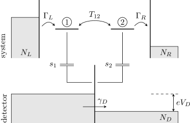
Figure 1: Quantum point contact in the tunnel regime acting as charge monitor for an undetuned but biased DQD. Electrons on the latter increase the tunnel barrier and, thus, reduce the detector current.

II Double quantum dot coupled to a charge detector

Our setup consists of a DQD formed by two single-level quantum dots in contact with electron source and drain. Since double occupation of the DQD is inhibited by Coulomb repulsion, spin effects play a minor role and will be ignored. This setup is described by the Hamiltonian $H_{\text{DQD}}+H_{\text{DQD,leads}}$, where

$$H_{\text{DQD}}=T_{12}(c_{1}^{\dagger}c_{2}+c_{2}^{\dagger}c_{1})$$ (1)

models the DQD with vanishing onsite energies, tunnel coupling $T_{12}$, and the fermionic operators $c_{\ell}$, where $\ell=1,2$. For ease of notation we use units with $e=\hbar=1$ and consider particle currents. We assume a large Coulomb repulsion such that at most one electron can reside on the DQD, which means that the only energetically accessible states are the empty state $|0\rangle$ and the single-electron states $|\ell\rangle$. The coupling to the electron source and drain is given by

$$H_{\text{DQD,leads}}=\sum_{q,\alpha}V_{q\alpha}(c_{\ell_{\alpha}}^{\dagger}c_{q\alpha}+c_{q\alpha}^{\dagger}c_{\ell_{\alpha}})+\sum_{q,\alpha}\epsilon_{q}N_{q\alpha},$$ (2)

where $c_{q\alpha}^{\dagger}$ are the fermionic creation operators for an electron in mode $q$ of lead $\alpha=L,R$ with the energy $\epsilon_{q}$. The mapping $\ell_{\alpha}$ takes the values $\ell_{L}=1$ and $\ell_{R}=2$, respectively. Tunneling between the DQD and the leads is determined by the spectral densities $\Gamma_{\alpha}(\epsilon)=(2\pi/\hbar)\sum_{q}|V_{q\alpha}|^{2}\delta(\epsilon-\epsilon_{q})\equiv\Gamma_{\alpha}$ which we assume within a wideband limit energy independent.

We restrict ourselves to a fully symmetric DQD with equal barrier capacitances. Then according to the Ramo-Shockley theorem,ShockleyJAP1938a ; BlanterPR2000a the displacement currents in the double dot circuit are such that the experimentally measured current is the average of the currents through the left and the right tunnel barrier, i.e., $I=\frac{1}{2}I_{L}-\frac{1}{2}I_{R}$. Its noise spectrum defined below depends on the charge fluctuations of the DQD and readsBlanterPR2000a ; MozyrskyPRB2002a ; MozyrskyPRB2002b

$$C_{II}(\omega)=\frac{1}{2}C_{I_{L}I_{L}}(\omega)+\frac{1}{2}C_{I_{R}I_{R}}(\omega)-\frac{\omega^{2}}{4}C_{NN}(\omega).$$ (3)

The charge detector is formed by a tunnel contact, see Fig. 1, and modeled by the Hamiltonian $H_{D}=\sum_{k}\epsilon_{k}c_{k}^{\dagger}c_{k}+\sum_{k^{\prime}}\epsilon_{k^{\prime}}c_{k^{\prime}}^{\dagger}c_{k^{\prime}}$ with the fermionic creation operators of the left and the right lead, $c_{k}^{\dagger}$ and $c_{k^{\prime}}^{\dagger}$, respectively. The tunnel coupling between the leads depends on the DQD occupation and readsGurvitzPRB1997a ; BraggioJSM2009a ; GolubevPRB2011a

$$H_{D}^{\text{tun}}=(1-s_{1}N_{1}-s_{2}N_{2})\sum_{kk^{\prime}}t_{kk^{\prime}}(c_{k}^{\dagger}c_{k^{\prime}}+c_{k^{\prime}}^{\dagger}c_{k}),$$ (4)

where $t_{kk^{\prime}}$ denotes the tunnel matrix elements which we replace in a continuum limit by the conductance $G(\epsilon,\epsilon^{\prime})=2\pi\sum_{kk^{\prime}}|t_{kk^{\prime}}|^{2}\delta(\epsilon-\epsilon_{k})\delta(\epsilon-\epsilon_{k^{\prime}})\equiv G_{D}$ in units of $e^{2}/h$, which is also assumed energy independent. The number operators $N_{\ell}$ in the prefactor reflect the fact that an electron on the DQD increases the potential barrier of the QPC and, thus, reduces the tunnel amplitudes. The strength of this reduction depends on the interaction with the DQD which is quantified by the dimensionless parameters $s_{1}$ and $s_{2}$. For consistency, it must obey $s_{1}N_{1}+s_{2}N_{2}\leq 1$ for all DQD occupations considered.

III DQD in the classical limit

Within a classical approximation, we assume that the inter-dot tunneling is small such that $H_{\text{DQD}}$ practically commutes with the occupation operators $N_{\ell}$. Then the DQD dynamics can be neglected for the computation of the tunnel rates. Thus, we can adopt the golden-rule treatment of Ref. Ingold1992a, by which we obtain that an electron in state $k$ of the left lead may tunnel to state $k^{\prime}$ of the right lead with probability $(2\pi/\hbar)|t_{kk^{\prime}}|^{2}\delta(\epsilon_{k}-\epsilon_{k^{\prime}})(1-s_{1}N_{1}-s_{2}N_{2})^{2}$. Expressing the probability for the initial many-body state in terms of Fermi functions and integrating over $\epsilon_{k}$ and $\epsilon_{k^{\prime}}$, we obtain that for $N_{1}=N_{2}=0$ the QPC current can be described by a Poisson process with a rate $\gamma_{0}=G_{D}|V_{D}|$ proportional to the bias voltage applied to the detector, $V_{D}$. Ingold1992a ; BlanterPR2000a If an electron resides on the DQD, Coulomb repulsion reduces the tunnel rates according to $\gamma_{0}\to\gamma\equiv\gamma_{0}(1-\tilde{s}_{1}N_{1}-\tilde{s}_{2}N_{2})$, where $\tilde{s}_{\ell}=s_{\ell}(2-s_{\ell})$ reflects the detector sensitivities.KohlerEPJB2013a

Subsuming these two cases, we can conclude that the QPC tunnel process inherits an additional randomness from the DQD occupation. In more technical terms, the Poisson process turns into a Cox process with a rate

$$\gamma=\gamma_{0}(1-\tilde{s}_{1}N_{1}-\tilde{s}_{2}N_{2})$$ (5)

which depends on the transport process of the DQD. Thus, the average current through the detector, $\langle j\rangle$, can be expressed in terms of the DQD occupations. While the same is true for the detector-DQD correlations, auto-correlations of the detector current contain also a (white) shot noise contribution, such that the power spectrum becomes BouzasAMM2006a

$$C_{jj}(\omega)=\langle j\rangle+\gamma_{0}^{2}\sum_{\ell,\ell^{\prime}=L,R}\tilde{s}_{\ell}\tilde{s}_{\ell^{\prime}}C_{N_{\ell}N_{\ell^{\prime}}}(\omega).$$ (6)

For an explicit derivation of the shot noise term, see Ref. MozyrskyPRB2002b, . The fluctuations of the detector current are characterized by the frequency-dependent Fano factor $F(\omega)=C_{jj}(\omega)/\langle j\rangle$. In consistency with Ref. KohlerEPJB2013a, , we find that good measurement correlations are accompanied by $F(\omega)\gg 1$, see Fig. 2(a) and discussion below.

III.1 Master equation for uni-directional transport

We consider a DQD with large bias such that electrons can enter exclusively from the left lead with tunnel rate $\Gamma_{L}$, while leaving to the right lead with tunnel rate $\Gamma_{R}$. For our numerical study, we focus on a symmetric situation with $\Gamma_{L}=\Gamma_{R}\equiv\Gamma$. Moreover, if the onsite energies of both dots are equal as well, inter-dot tunneling is direction independent with a rate $\Gamma_{12}\ll\Gamma$. The restriction to small rates ensures that inter-dot tunneling is incoherent and, thus, consistent with the classical description.

If at most one electron can reside in the DQD, we have to take into account the states $0$, $1$, and $2$, referring to an empty DQD and one electron in the left or the right dot, respectively. Then the corresponding occupation probabilities obey the master equation $\dot{P}=\mathcal{M}P$, with

$$\mathcal{M}=\begin{pmatrix}-\Gamma_{L}&0&\Gamma_{R}\\ \Gamma_{L}&-\Gamma_{12}&\Gamma_{12}\\ 0&\Gamma_{12}&-\Gamma_{12}-\Gamma_{R}\end{pmatrix},$$ (7)

and $P=(P_{0},P_{1},P_{2})^{\mathsf{T}}$, where $\mathsf{T}$ denotes transposition and $\ell=0,1,2$ labels the charge states of the DQD. $P^{\text{st}}$ denotes with $\mathcal{M}P^{\text{st}}=0$ the stationary solution of the master equation. Our central quantity for the computation of correlation functions is the conditional probability

$$P(\ell,t|\ell^{\prime},t^{\prime})=[e^{\mathcal{M}(t-t^{\prime})}]_{\ell\ell^{\prime}},$$ (8)

for the DQD being in state $\ell$ at time $t$ provided that it was in state $\ell^{\prime}$ at the earlier time $t^{\prime}<t$. It is equivalent to the propagator of the master equationRisken1989a and obeys $P(\ell,t+dt|\ell^{\prime},t)=\delta_{\ell\ell^{\prime}}+\mathcal{M}_{\ell\ell^{\prime}}dt$.

III.2 DQD-detector correlations

The correlation of any DQD variable $X$ with the detector current $j$ can be obtained from the stochastic part of the rate $\gamma$ given by Eq. (5) and reads

$$C_{jX}=-\gamma_{0}(\tilde{s}_{1}C_{N_{1}X}+\tilde{s}_{2}C_{N_{2}X}).$$ (9)

Since we are interested in the degree of correlation rather than in absolute values, we focus on the normalized correlation at a given measurement frequency $\omega$ which we define as

$$r_{ab}(\omega)=\frac{C_{ab}(\omega)}{\sqrt{C_{aa}(\omega)\,C_{bb}(\omega)}}\,.$$ (10)

Its absolute value is a figure of merit for the detection quality and in the ideal case is of order unity. In turn, for $|r_{jX}|\ll 1$, the detector current is practically independent of $X$.

In order to quantify the detection of the charge in dot $\ell=1,2$, we consider the correlation coefficient $r_{jN_{\ell}}$. According to Eqs. (6) and (9), it can be expressed in terms of the DQD correlation functions of the populations which in the time domain read

$$C_{N_{\ell}N_{\ell^{\prime}}}(t-t^{\prime})=\langle N_{\ell}(t)N_{\ell^{\prime}}(t^{\prime})\rangle-\langle N_{\ell}\rangle\langle N_{\ell^{\prime}}\rangle.$$ (11)

Since $N_{\ell}$ can assume only the values 0 and 1, the first term on the right-hand side is given by the joint probability $P(\ell,t;\ell^{\prime},t^{\prime})$ for the DQD being in the states $\ell$ and $\ell^{\prime}$ at the respective times. Bayes’ theorem relates this joint probability in the stationary limit to $P^{\text{st}}$ and the conditional probability (8) so that we obtain for $t\geq t^{\prime}$ the expression

$$C_{N_{\ell}N_{\ell^{\prime}}}(t-t^{\prime})=P(\ell,t|\ell^{\prime}t^{\prime})P_{\ell^{\prime}}^{\text{st}}-P_{\ell}^{\text{st}}P_{\ell^{\prime}}^{\text{st}},$$ (12)

while the opposite time ordering $t<t^{\prime}$ follows by relabeling.

In order to obtain the correlation of the detector current with the DQD currents, we use Eq. (9) to write the detector current in terms of the DQD occupations and obtain $\langle N_{1}(t)I_{R}(t^{\prime})\rangle$, as well as similar expressions with other combination of the indices $1$, $2$ and $L$, $R$. Following Refs. KorotkovPRB1994a, ; KohlerEPJB2013a, we define the differential $dN_{R}(t)=I_{R}(t)dt$ which describes the change of the charge state in the right dot by a current flow to the leads. Then we express the probabilities of all trajectories that contribute to $\langle N_{1}(t)I_{R}(t^{\prime})\rangle dt=\langle N_{1}(t)dN_{R}(t^{\prime})\rangle$ by the conditional probability (8).

For $t^{\prime}<t$, the only contribution to the mentioned term stems from a trajectory starting at time $t^{\prime}$ with an electron on the right dot which leaves during the infinitesimal time $dt$ to the right lead, such that the DQD will be in state $0$. At a later time $t$, the left lead must be occupied. For the opposite time ordering, the DQD starts at time $t^{\prime}$ in state $1$, propagates to state $2$ at time $t$, while then an electron leaves to the right dot during $dt$. The joint probability for these events reads

$$\langle dN_{R}(t)N_{1}(t^{\prime})\rangle$$

$$=\begin{cases}P(0,t+dt|2,t)P(2,t|1,t^{\prime})P_{1}^{\text{st}},&t>t^{\prime}\\ P(1,t^{\prime}|0,t)P(0,t+dt|2,t)P_{2}^{\text{st}},&t<t^{\prime}\end{cases}.$$ (13)

The auto-correlation function of the DQD current at the right barrier requires an initial occupation of state $2$ at $t^{\prime}$, tunneling to the right lead during $dt$, propagation from $0$ to $2$ during $t-t^{\prime}$, and finally electron tunneling to the right lead. This happens with probability

$$\begin{split}\langle dN_{R}(t)dN_{R}(t^{\prime})\rangle={}&P(0,t+dt|2,t)P(2,t|0,t^{\prime})\\ &\times P(0,t^{\prime}+dt|2,t^{\prime})P_{2}^{\text{st}},\end{split}$$ (14)

valid for $t^{\prime}<t$ while the opposite time ordering again follows by relabeling. At equal times, we have to add the shot noise contribution to obtain $C_{I_{R}I_{R}}(t-t^{\prime})=\langle dN_{R}(t)dN_{R}(t^{\prime})\rangle/dt^{2}+\langle I_{R}\rangle\delta(t-t^{\prime})$. A derivation of the shot noise in the spirit of the present calculation can be found in Ref. KorotkovPRB1994a, .

The correlation functions for all other possible combinations of the indices $L$ and $R$ can be obtained in the same way and are listed in Appendix A.

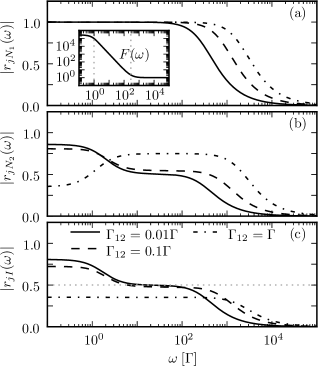
Figure 2: Classical frequency-dependent correlation coefficients between the detector current and (a) the occupation of the left dot, (b) the occupation of the right dot, and (c) the symmetrized current through the DQD for various inter-dot rates $\Gamma_{12}$. The detector is characterized by a bare rate $\gamma_{0}=10^{8}\Gamma$ and the sensitivities $\tilde{s}_{1}=0.2$ and $\tilde{s}_{2}=0$, i.e., it couples to only the left dot. The inset in panel (a) shows the frequency dependent Fano factor of the detector current for $\Gamma_{12}=0.01\>\Gamma$, where the dashed lines mark the crossover region between the plateaus. The horizontal line in panel (c) marks the upper limit $1/2$ discussed in the text.

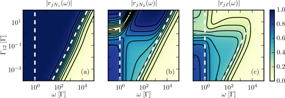
Figure 3: Classical correlation coefficients depicted in Fig. 2 as function of the frequency $\omega$ and the inter-dot rate $\Gamma_{12}$ while all other parameters are the same. The dashed lines at $\omega=\Gamma$ and at $\omega=\omega_{\text{max}}$ mark the crossover between the different regimes discussed in the text.

III.3 Numerical results

For the numerical evaluation of the correlation coefficients, we diagonalize the matrix (7) to obtain a bi-orthonormal set of left and right eigenvectors, $u_{i}^{\mathsf{T}}$ and $v_{i}$, as well as the eigenvalues $-\lambda_{i}$, so that $\exp(\mathcal{M}t)=\sum_{i}v_{i}u_{i}^{\mathsf{T}}e^{-\lambda_{i}t}$ for $t>0$. In doing so, we obtain for each correlation function a sum of decaying exponentials and a formal expression for the Fourier transformed of the propagator $P(\ell,t|\ell^{\prime},0)$. We restrict ourselves to a symmetric DQD with $\Gamma_{L}=\Gamma_{R}\equiv\Gamma$. Then the latter parameter determines the frequency scale of the DQD dynamics.

Investigating various correlation functions, we found that one has to distinguish three frequency regimes which can be characterized by the frequency-dependent Fano factor of the detector current derived in Appendix B and depicted in the inset of Fig. 2(a). First, if the measurement frequency is small, $\omega\lesssim\Gamma$, all correlation functions assume their zero-frequency value. Typically the detector Fano factor is several orders of magnitude above the shot noise level, where its precise value depends much on the coupling strengths $\tilde{s}_{1}$ and $\tilde{s}_{2}$. Such low measurement frequencies correspond to static DQD properties, i.e., time-averaged expectation values. The crossover to the high-frequency limit occurs at

$$\omega_{\text{max}}=(2\gamma_{0}\Gamma_{12})^{1/2}\max(\tilde{s}_{1},\tilde{s}_{2}),$$ (15)

which reflects the largest relevant frequency. For $\omega\gtrsim\omega_{\text{max}}$, the Fano factor assumes the Poissonian value $F(\omega)\approx 1$ while all DQD-detector correlations practically vanish. Thus, on such large frequency scales and on the corresponding short time scales, the detector cannot provide information about the DQD. The proportionality of the upper limit, $\omega_{\text{max}}\propto\gamma_{0}^{1/2}$, has also been found for detecting the charge of a single quantum dot.KohlerEPJB2013a In the intermediate regime, we find $F(\omega)\propto\omega^{-2}$. There the correlation coefficients provide information about the possibility of time-resolved measurement. This generic global behavior of the detector-DQD correlations relates the possibility of charge detection to the emergence of super-Poissonian detector noise. Physically, this reflects switching between two values of the detector current and the associated bunching of the electrons flowing through the detector.

III.3.1 Charge detection

Figures 2 and 3 show the correlations between the detector current $j$ and the DQD for the coupling to only the left quantum dot. Then for frequencies below $\omega_{\text{max}}$, the measurement correlation with the occupation of the left dot (panel a in both figures) assumes the ideal value $r_{jN_{1}}=1$. This indicates the possibility of time-resolved detection of the charge on the left dot, as long as the Fano factor stays significantly above the shot noise. Thus the time resolution of the present charge detection scheme is determined by Eq. (15).

Since an electron on the right quantum dot originates from the left lead, it must have occupied the left dot at some earlier stage. Then one naturally expects some remnant correlation between the occupations of both dots. As a consequence, the detector not only correlates with the dot to which it couples, but also with the other dot as can be appreciated in Figs. 2(b) and 3(b). In the regime of weak inter-dot tunneling, $\Gamma_{12}\lesssim\Gamma$, this correlation decays as a function of $\omega$ via an intermediate plateau limited by the crossover frequencies $\Gamma$ and $\omega_{\text{max}}$. For $\omega\lesssim\Gamma$, we find $r_{jN_{2}}\approx 0.8$, i.e., the average population of dot 2 can be noticed to some extent. In the intermediate regime, $\Gamma\lesssim\omega\lesssim\omega_{\text{max}}$, the correlation coefficient drops down to a value $1/2$. Interestingly enough, for a strong inter-dot rate $\Gamma_{12}\gtrsim\Gamma$, the intermediate plateau becomes larger than in the zero-frequency limit, but the correlation coefficient always stays clearly below unity.

In a realistic setup, a charge detector at a DQD is sensitive not only to the closer dot, but to some extent also to the other dot. This raises the question whether the influence of the latter affects the measurement quality. Being interested in time-resolved measurement, we focus on the intermediate frequency regime. Figure 4(a) shows the correlation coefficient of the detector current with the occupation of the left dot as a function of both sensitivities. It demonstrates that (almost) perfect correlation requires $\tilde{s}_{1}\gtrsim 2\tilde{s}_{2}$, i.e., the left dot must couple at least twice as strong as the right dot. An extreme case of very small correlation is found for $\tilde{s}_{2}\approx 2\tilde{s}_{1}$. There the behavior is even counter-intuitive since reducing further the coupling to the left dot increases the correlation. Finally, the correlation with the population of the right dot (not shown) behaves accordingly. It can be obtained by interchanging the labels 1 and 2, which is non-trivial since reflection symmetry is absent owing to the bias voltage applied to the DQD.

III.3.2 Current detection

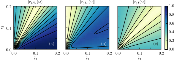
Figure 4: Classical correlation coefficients between the detector and (a) the occupation of the left dot, (b) the current through the left DQD barrier, and (c) the Ramo-Shockley current as a function of the detector sensitivities $\tilde{s}_{1}$ and $\tilde{s}_{2}$. The frequency $\omega=50\Gamma$ corresponds to the middle of the second plateau at which time-resolved measurement is possible. The inter-dot rate is $\Gamma_{12}=0.1\Gamma$, while all other parameters are as in Fig. 2.

Even though the detector couples to the charge degree of freedom, it has been employed to reconstruct the corresponding time-resolved current GustavssonPRL2006a ; FrickePRB2007a and its full-counting statistics.FlindtPNASUSA2009a A later theoretical investigation KohlerEPJB2013a revealed that nevertheless the correlation coefficient between the detector current and the measured current is significantly smaller than unity. Thus, knowledge about the transport mechanism must provides missing information.

Figure 4(b) depicts the correlation of the detector current with the current entering the DQD from the left lead at an intermediate measurement frequency. It assumes its maximum $r_{jI_{L}}\approx 0.8$ for $\tilde{s}_{1}\approx 2\tilde{s}_{2}$. Surprisingly, this value is slightly above the limit of $\sqrt{1/2}$ found for a detector coupled to a single quantum dot.KohlerEPJB2013a A remarkable difference to the single quantum dot is also found for the Ramo-Shockley current $I=\frac{1}{2}I_{L}-\frac{1}{2}I_{R}$ which for a symmetric single quantum dot is fully uncorrelated with the detector current.KohlerEPJB2013a Figure 4(c), by contrast, reveals that this is not the case for a DQD unless both dots couple equally strongly to the detector. If one coupling dominates, the correlation can be up to $r_{jI}=1/2$.

IV Quantum mechanical description

In order to obtain the quantum mechanical detector-DQD correlations, we employ a Bloch-Redfield master equation RedfieldIBMJRD1957a augmented by a counting variable BagretsPRB2003a that allows the computation of higher-order moments. Since this master equation is Markovian, one can compute two-time expectation values of system variables via the quantum regression theorem.LaxPR1963a ; LaxPR1967a ; Carmichael2002a In contrast to previous applications of this approach to quantum transport, EmaryPRB2007a ; MarcosNJP2010a ; UbbelohdeNC2012a the detector current operator is not a usual “electron jump term” between the system and a lead, which requires a generalization of the formalism. For the derivation we follow Ref. HusseinPRB2014a, .

IV.1 Bloch-Redfield master equation

We start from the full DQD-lead-detector Hamiltonian and separate it into the DQD contribution $H_{S}$ given by Eq. (1), the lead terms, and the tunneling from and to the four leads are involved. After transforming the Liouville-von Neumann equation for the total density operator into the interaction picture with respect to the local terms, we derive a master equation that captures the lead tunneling to second-order. Next, we multiply the full density operator with the $e^{i\bm{\chi}\bm{N}}$, where ${\bm{\chi}}=\{\chi_{L},\chi_{R},\chi_{D}\}$ contains the counting variables for the left and the right lead of the DQD and for the right lead of the detector, respectively. Notice that owing to charge conservation, one counting variable for the detector is sufficient. The vector $\bm{N}$ contains the corresponding lead electron numbers. By tracing out the leads, we obtain the master equation $\dot{\rho}=\mathcal{L}({\bm{\chi}})\rho$ with the generalized Liouvillian $\mathcal{L}({\bm{\chi}})\rho=-i[H_{S},\;\rho]+\mathcal{L}_{S}({\bm{\chi}})\rho+\mathcal{L}_{D}({\bm{\chi}})\rho$. The generalized density operator $\rho$ relates to the moment-generating function for the lead electrons as $\operatorname{tr}\rho=\langle e^{i\bm{\chi}\bm{N}}\rangle$. For DQD-lead tunneling in the large-bias limit, we find

$$\mathcal{L}_{S}({\bm{\chi}})\rho={} \Gamma_{L}\big{[}D(c^{\dagger}_{L})\rho+(e^{-i\chi_{L}}-1)c^{\dagger}_{L}\rho c_{L}\big{]}$$

$$+\Gamma_{R}\big{[}D(c_{R})\rho+(e^{i\chi_{R}}-1)c_{R}\rho c^{\dagger}_{R}\big{]}$$ (16)

with the Lindblad operator $D(x)\rho=x\rho x^{\dagger}-\{x^{\dagger}x,\;\rho\}/2$.

The tunnel Hamiltonian of the detector, Eq. (4), contains besides lead terms the system operator $X\equiv\openone-\sum_{\ell}s_{\ell}N_{\ell}$ which determines the generalized detector Liouvillian

$$\mathcal{L}_{D}(\bm{\chi})\rho={} Y_{-}(\bm{\chi})\rho X+X\rho Y_{+}(\bm{\chi})-XY_{-}\rho-\rho Y_{+}X,$$ (17)

where in the zero-temperature limit and for large bias voltage, $|V_{D}|>2|T_{12}|$,

$$Y_{\pm}(\bm{\chi}) =e^{i\chi_{D}\operatorname{sgn}V_{D}}\frac{G_{D}}{2}\big{(}|V_{D}|X\pm[H_{S},\;X]\big{)}.$$ (18)

The commutator in Eq. (18) is proportional to the inter-dot tunnel amplitude $T_{12}$ and, thus, can be neglected for large detector bias voltage, $|V_{D}|\gg 2|T_{12}|$. Therefore, we proceed with

$$\mathcal{L}_{D}(\bm{\chi})\rho={} \gamma_{0}\big{[}D(X)\rho+(e^{i\chi_{D}\operatorname{sgn}V_{D}}-1)X\rho X\big{]},$$ (19)

where $\gamma_{0}=G_{D}|V_{D}|$ is the tunnel rate of the detector in the absence of the DQD. For typical parameters GustavssonPRL2006a ; FrickePRB2007a ; IhnSSC2009a of $V_{D}=1\,\textrm{mV}$, $G_{D}\lesssim 0.1\,e^{2}/h$, DQD-lead rates $\Gamma$ of a few kHz, and inter-dot tunneling up to $T_{12}=100\,\mu\mathrm{eV}$, this corresponds to detector rates in the range of $10^{5}$–$10^{8}\,\Gamma$.

IV.2 Charge and current correlations

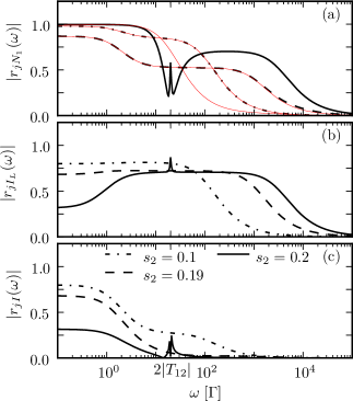
Figure 5: Quantum mechanical version of the correlation coefficients between the detector current and (a) the occupation of the left dot, (b) the current through the left DQD barrier, and (c) the symmetrized current through the DQD for various values of the sensitivity $s_{2}$ while $s_{1}=0.2$ is fixed. The inter-dot tunnel coupling is $T_{12}=10\Gamma$, while all other parameters are as in Fig. 2. The thin red lines in panel (a) show the corresponding classical correlation coefficients for $\Gamma_{12}$ determined by the quantum-to-classical mapping in Eq. (26).

Also here we characterize the measurement by normalized correlation coefficients defined in Eq. (10), but with the corresponding quantum mechanical expressions on the right-hand side. Thus, we have to compute auto-correlations and cross correlations of the DQD occupations and the detector current.

For the dot occupations, we define $C_{N_{\ell}N_{\ell^{\prime}}}$ as in Eq. (11). From the quantum regression theorem LaxPR1963a ; LaxPR1967a ; Carmichael2002a follows the frequency-dependent correlation function

$$C_{N_{\ell}N_{\ell^{\prime}}}(\omega)=\operatorname{tr}[N_{\ell}\mathcal{R}(-i\omega)N_{\ell^{\prime}}\rho_{\textrm{st}}+N_{\ell^{\prime}}\mathcal{R}(i\omega)\rho_{\textrm{st}}N_{\ell}].$$ (20)

In order to formally perform the Fourier transformation, we have introduced the pseudoresolvent $\mathcal{R}(z)=\mathcal{Q}(z-\mathcal{L})^{-1}\mathcal{Q}$ with $\mathcal{Q}=(\openone-\rho_{\textrm{st}}\operatorname{tr})$ the projector to the part of Liouville space orthogonal to the stationary state $\rho_{\textrm{st}}$ of the DQD.

In contrast to the classical case, our master equation formalism allows us to treat all currents on equal footing, namely by computing derivatives of the generalized Liouvillian $\mathcal{L}(\bm{\chi})$ with respect to the corresponding counting variable. Proceeding as in Refs. EmaryPRB2007a, ; MarcosNJP2010a, ; UbbelohdeNC2012a, , we find

$$C_{I_{\alpha}I_{\beta}}(\omega)=\langle\mathcal{W}_{\alpha\beta}\rangle+\langle\mathcal{W}_{\alpha}\mathcal{R}(-i\omega)\mathcal{W}_{\beta}\rangle+\langle\mathcal{W}_{\beta}\mathcal{R}(i\omega)\mathcal{W}_{\alpha}\rangle,$$ (21)

where $\alpha,\beta\in\{L,R,D\}$ label the leads. The superoperators $\mathcal{W}_{\alpha}=(\partial\mathcal{L}/\partial i\chi_{\alpha})|_{\bm{\chi}=\bm{0}}$ and $\mathcal{W}_{\alpha\beta}=(\partial^{2}\mathcal{L}/\partial i\chi_{\alpha}\partial i\chi_{\beta})|_{\bm{\chi}=\bm{0}}$ are Taylor coefficients of $\mathcal{L}(\bm{\chi})$, where the first order provides the average currents $I_{\alpha}=\langle\mathcal{W}_{\alpha}\rangle$. Formally, expression (21) follows by substituting in Eq. (20) the number operators by jump operators and adding the shot noise contribution $\langle\mathcal{W}_{\alpha\beta}\rangle$ which vanishes unless $\alpha=\beta$.

The frequency-dependent fluctuations (3) of the Ramo-Shockley current ShockleyJAP1938a ; BlanterPR2000a $I=\frac{1}{2}I_{L}-\frac{1}{2}I_{R}$ are linear combination of the above expressions. They can also be obtained directly from the generalized density operator by transforming the counting fields according to MarcosNJP2010a $\chi_{L}\to\chi_{A}+\chi_{T}/2$ and $\chi_{R}\to\chi_{A}-\chi_{T}/2$, where $\chi_{T}$ refers to the total current and $\chi_{A}$ accounts for temporary charge accumulation on the DQD. Notice that we follow the sign convention of Ref. JinNJP2013a, , where the currents are positive when electrons flow from the lead to the DQD.

For the cross correlations between currents and DQD occupations, we define the according expression

$$C_{I_{\alpha}N_{\ell}}(\omega)=\operatorname{tr}[N_{\ell}\mathcal{R}(-i\omega)\mathcal{W}_{\alpha}\rho_{\textrm{st}}+\mathcal{W}_{\alpha}\mathcal{R}(i\omega)\rho_{\textrm{st}}N_{\ell}].$$ (22)

Since we did not derive the latter correlation function in terms of a measurement procedure, it is an operationally defined quantity rather than an observable. For ease of notation we henceforth replace the subscript $I_{D}$ by $j$.

IV.3 Classical limit of the quantum master equation

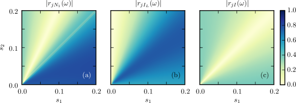
Figure 6: Quantum mechanical version of the correlation coefficients shown in Fig. 4 as a function of the detector sensitivities $s_{1}$ and $s_{2}$. The frequency is $\omega=50\Gamma$, the tunnel rate is $T_{12}=10\Gamma$, while all other parameters are as in Fig. 5. Notice that in the regime depicted, the classical and the quantum mechanical detector sensitivities relate as $s_{\ell}\approx\tilde{s}_{\ell}/2$.

The classical limit of the Bloch-Redfield equation can be obtained by eliminating the coherences between the left and the right quantum dot in the limit of small inter-dot tunneling $T_{12}$. This task is hampered by the fact that the natural basis of the Bloch-Redfield equation is given by the eigenstates of $H_{S}$ which, owing to the absence of a detuning, are always delocalized irrespective of how small $T_{12}$ is. However, there exists a way out based on the comparison of the average currents in both limits. While comparing the DQD currents yields an effective $\Gamma_{12}$ in terms of $T_{12}$, the detector current provides a relation between the coupling strengths of the quantum mechanical model, $s_{\ell}$, and the classical couplings $\tilde{s}_{\ell}$.

A straightforward computation of the stationary state of the classical master equation, see Eq. (7), yields the occupation numbers

$$\langle N_{1}\rangle =\frac{\Gamma_{L}(\Gamma_{R}+\Gamma_{12})}{\Gamma_{L}\Gamma_{R}+(2\Gamma_{L}+\Gamma_{R})\Gamma_{12}},$$ (23)

$$\langle N_{2}\rangle =\frac{\Gamma_{L}\Gamma_{12}}{\Gamma_{L}\Gamma_{R}+(2\Gamma_{L}+\Gamma_{R})\Gamma_{12}},$$ (24)

from which by use of $I_{\text{DQD}}^{\text{cl}}=\Gamma_{R}\langle N_{2}\rangle$ immediately follows

$$I_{\text{DQD}}^{\text{cl}} =\frac{\Gamma_{L}\Gamma_{R}\Gamma_{12}}{\Gamma_{L}\Gamma_{R}+(2\Gamma_{L}+\Gamma_{R})\Gamma_{12}}.$$ (25)

Comparison with the corresponding expression for the quantum master equation, $\langle\mathcal{W}_{R}\rangle$, provides the effective classical inter-dot rate

$$\Gamma_{12}=\frac{4|T_{12}|^{2}}{\Gamma_{R}+\gamma_{0}(s_{1}-s_{2})^{2}}.$$ (26)

Obviously, the DQD current assumes its maximum for $s_{1}=s_{2}$, while it becomes much smaller when the two couplings are different (notice that typically $\gamma_{0}\ggg\Gamma_{L,R}$). The reason for this current reduction is the fact that for $s_{1}\neq s_{2}$, the detector performs a position measurement of the DQD electrons. Therefore, it destroys the coherence between the left dot and the right dot and, thus, forces the electron into the corresponding eigenstates, which leads to localization. This localization is manifest in a current suppression which represents the main measurement backaction of the charge sensor to the DQD. In the limiting case $s_{1}=s_{2}$, the measured quantity is the total electron number of the DQD which commutes with $H_{S}$ and therefore does not affect the coherences. Below we will find that in a large part of parameter space, the classical treatment with $\Gamma_{12}$ given by Eq. (26) agrees very well with the full quantum mechanical solution.

For the detector current, we insert the populations (23) and (24) into Eq. (5) to obtain

$$j_{\text{cl}} =G_{D}V_{D}(1-\tilde{s}_{1}\langle N_{1}\rangle-\tilde{s}_{2}\langle N_{2}\rangle),$$ (27)

where the prefactor relates to the tunnel rate of the detector, $\gamma_{0}=G_{D}|V_{D}|$. Comparison with the quantum mechanical expression and using the above result for $\Gamma_{12}$ provides a relation between the classical and the quantum mechanical detector sensitivities,

$$\tilde{s}_{\ell}=s_{\ell}(2-s_{\ell}),$$ (28)

where for the small couplings considered in our numerical studies, $\tilde{s}_{\ell}\approx 2s_{\ell}$.

IV.4 Numerical results

We already discussed above that the presence of the detector causes backaction which reduces the effective inter-dot rate $\Gamma_{12}$. In particular, this rate becomes smaller with a larger difference between the two detector couplings, $|s_{1}-s_{2}|$. Consequently, we expect that the frequency $\omega_{\text{max}}$ beyond which all DQD-detector correlations vanish [see Eq. (15)] also depends on the coupling strength as well as on the bare detector rate $\gamma_{0}$. The quantum mechanical correlation coefficients for different values of $s_{2}$ depicted in Fig. 5 confirm this expectation.

IV.4.1 Charge detection

Figures 5(a) and 6(a) show the correlation coefficient between the occupation of the left quantum dot and the detector current. The former is compared with the classical result with the effective $\Gamma_{12}$ given by Eq. (26). We find that as long as the two couplings are different, the values obtained from the quantum-to-classical mapping are practically the same as those of the quantum case. A minor difference is visible at large frequencies for $s_{2}=0.19$. Only when both couplings are equal, the quantum mechanical solution becomes rather different and is beyond the classical approach. This corresponds to the situation discussed above in which the detector is sensitive to the total number of electrons on the DQD. Then the DQD-detector Hamiltonian commutes with $H_{S}$ and, thus, it measures a good quantum number.

This behavior is also found for the correlation for an intermediate frequency as a function of the couplings shown in Fig. 6(a). The main difference to the corresponding classical solution (not shown) is found in a narrow region at $s_{1}=s_{2}$. As in the classical case, fulfilling the condition for good charge detection at dot 1, $r_{jN_{1}}\approx 1$, requires $s_{1}\gtrsim 2s_{2}$.

IV.4.2 Current detection

Figure 5 also shows the correlation coefficients with the DQD current through the left barrier (panel b) and with the Ramo-Shockley current (panel c). Besides the global behavior already discussed for the correlation with the DQD occupations, we find for $s_{1}=s_{2}$ a sharp peak at a measurement frequency $2|T_{12}|$ which corresponds to the level splitting of the DQD. As soon as both couplings differ minimally, this peak vanishes. Since we consider $\gamma_{0}\ggg\Gamma$, a tiny difference of much less than one percent is already sufficient to suppress the peak. This demonstrates that the detector by and large destroys the quantum features of the DQD unless it couples to a good quantum number.

Panels b and c of Fig. 6 show the correlations of the detector and the DQD currents as a function of the sensitivities for an intermediate frequency. It confirms the predictions from the classical treatment (cf. the corresponding panels of Fig. 4). In particular, it shows that also quantum mechanically the current through the individual barriers may correlate strongly with the detector, while the Ramo-Shockley always correlates weakly.

V Conclusions

We have studied a tunnel contact employed as charge sensor for a strongly biased DQD such that electrons are detected while being transported. The central idea of this scheme is a capacitive coupling between the two subsystems by which electrons on the DQD reduce the transmission of the tunnel contact. We have characterized this measurement by correlation coefficients of the detector current and DQD observables both in the classical limit and within a full quantum mechanical approach. The comparison of these limits allowed us to investigate the backaction on the coherence of DQD electrons.

A key ingredient to the classical description is a phenomenological incoherent inter-dot transition rate that enters the master equation for the DQD populations. It determines the conditional probabilities of the DQD and, thus, the joint probabilities that enter the two-time correlations under investigation. This approach represents a generalization of the one used for calculating current-current correlations KorotkovPRB1994a and measurement correlations KohlerEPJB2013a for a single electron transistor.

The correlation coefficients studied provide a limiting frequency beyond which measurement is no longer possible and which determines the time-resolution of the detection scheme. This limit increases with the detector rate, the inter-dot rate, and the detector sensitivity. The possibility of charge detection depends also crucially on the ratio between the capacitive couplings to each dot: A charge on a particular dot can be monitored reliably only if it couples to the detector at least twice as strong as an electron on the other dot. With the time-resolved DQD populations at hand, one can reconstruct the corresponding time-dependent current, at least under the assumption of unidirectional transport. This is reflected by a significant, but not perfect correlation between the detector and the DQD currents. Rather surprisingly, it is slightly larger than for the corresponding setup with a single-electron transistor, despite the more complicated transport mechanism of the present case.

On the quantum mechanical level, we used a method based on a Bloch-Redfield master equation augmented by a counting field.EmaryPRB2007a ; MarcosNJP2010a In order to capture also the detector current, we generalized this method to the presence of “jump terms” that do not alter the DQD occupation, but describe the detector current. A main issue for such quantum mechanical position measurement is its backaction to the coherence of the measured system. In the present case it is manifest in an additional localization of the DQD electrons. On the one hand, this leads to a significant reduction of the DQD current, on the other hand, it pushes the system towards its classical limit. Indeed our quantitative analysis revealed that the classical description is adequate whenever the detector current correlates strongly with one of the DQD occupations. A natural expectation is that this tendency should be even stronger in the presence of couplings to external degrees of freedom such as the electronic circuitry or substrate phonons.

Even though we restricted ourselves to a narrow part of parameter space, we observed a rather rich behavior. Thus, a full understanding of the detection scheme may require to take further ingredients into account. Besides the already mentioned influence of external degrees of freedom, this could be a detuning which leads to additional localization.

Appendix A Conditional probabilities and correlation functions

In Sec. IV.2, we explicitly derived the correlation functions $C_{I_{R}N_{1}}$ and $C_{I_{R}I_{R}}$, see Eqs. (III.2) and (14). For completeness, we here sketch the derivation of all other expressions required for the evaluation of the correlation coefficients discussed in the main text.

As discussed above, correlations between DQD occupations and DQD current from lead $\alpha=L,R$ can be expressed by the differential $dN_{\alpha}=I_{\alpha}dt$ and joint probabilities. For the currents through the left and the right contact, we thus obtain

$$\langle I_{L}\rangle dt={} \langle dN_{L}(t)\rangle=P(1,t+dt|0,t)P_{0}^{\text{st}},$$ (29)

$$\langle I_{R}\rangle dt={} \langle dN_{R}(t)\rangle=P(0,t+dt|2,t)P_{2}^{\text{st}},$$ (30)

where we find in consistency with charge conservation $\langle I_{L}\rangle=\langle I_{R}\rangle$.

The two-time correlations follow from the conditional probability (8) and Bayes’ theorem which yields

$$\langle N_{1}(t)dN_{L}(t^{\prime})\rangle$$ (31)

$$=\begin{cases}P(1,t^{\prime}+dt|0,t^{\prime})P(0,t^{\prime}|1,t)P_{1}^{\text{st}},&t<t^{\prime}\\ P(1,t|1,t^{\prime}+dt)P(1,t^{\prime}+dt|0,t^{\prime})P_{0}^{\text{st}},&t>t^{\prime}\end{cases},$$

$$\langle N_{2}(t)dN_{L}(t^{\prime})\rangle$$ (32)

$$=\begin{cases}P(1,t^{\prime}+dt|0,t^{\prime})P(0,t^{\prime}|2,t)P_{2}^{\text{st}},&t<t^{\prime}\\ P(2,t|1,t^{\prime}+dt)P(1,t^{\prime}+dt|0,t^{\prime})P_{0}^{\text{st}},&t>t^{\prime}\end{cases},$$

$$\langle N_{2}(t)dN_{R}(t^{\prime})\rangle$$ (33)

$$=\begin{cases}P(0,t^{\prime}+dt|2,t^{\prime})P(2,t^{\prime}|2,t)P_{2}^{\text{st}},&t<t^{\prime}\\ P(2,t|0,t^{\prime}+dt)P(0,t^{\prime}+dt|2,t^{\prime})P_{2}^{\text{st}},&t>t^{\prime}\end{cases}.$$

Subtracting $\langle N_{\ell}\rangle\langle dN_{\ell^{\prime}}\rangle$ and dividing by $dt$ yields the desired occupation-current correlations.

Accordingly, the correlation function of the left DQD current can be expressed in terms of

$$\langle dN_{L}(t)dN_{L}(t^{\prime})\rangle$$ (34)

$$=P(1,t+dt|0,t)P(0,t|1,t^{\prime}+dt)P(1,t^{\prime}+dt|0,t^{\prime})P_{0}^{\text{st}}.$$

Notice that this expression provides the auto-correlation function $C_{I_{L}I_{L}}(t-t^{\prime})$ only for $t\neq t^{\prime}$, while for equal times, the shot noise contribution $\langle I_{L}\rangle\delta(t-t^{\prime})$ must be added. KorotkovPRB1994a

Appendix B Alternative solution of the classical model and Fano factor

The numerical method for computing the quantum mechanical correlation functions in Sec. III can be employed as well for the classical limit. The classical master equation is formally an equation of motion for the diagonal matrix elements of the density matrix in the localized basis. Since in the DQD Liouvillian the dissipative term that describes the influence of the detector, see Eq. (19), is also diagonal in this basis, we merely have to replace the augmented Liouvillian $\mathcal{L}(\bm{\chi})$ by

$$\mathcal{M}({\bm{\chi}})={} \mathcal{M}+\Gamma_{L}(e^{-i\chi_{1}}-1)\mathcal{J}_{L}+\Gamma_{R}(e^{i\chi_{2}}-1)\mathcal{J}_{R}$$

$$+\gamma_{0}(e^{i\chi_{D}\operatorname{sgn}V_{D}}-1)\mathcal{J}_{D}$$ (35)

with $\mathcal{M}$ as in Eq. (7) and the DQD-lead jump operators

$$\mathcal{J}_{L}=\begin{pmatrix}0&0&0\\ 1&0&0\\ 0&0&0\end{pmatrix},\qquad\mathcal{J}_{R}=\begin{pmatrix}0&0&1\\ 0&0&0\\ 0&0&0\end{pmatrix},$$ (36)

while the detector jump operator

$$\mathcal{J}_{D}=\begin{pmatrix}1&0&0\\ 0&1-\tilde{s}_{1}&0\\ 0&0&1-\tilde{s}_{2}\end{pmatrix}$$ (37)

follows from Eq. (19) by ignoring non-diagonal contributions. We have confirmed all results of Sec. III with this method.

This alternative method is rather convenient for obtaining an analytical expression for the detector Fano factor in the classical limit. For this purpose, we compute the pseudoresolvent of $\mathcal{M}$ so that we can directly evaluate the auto-correlation function of the detector, $C_{jj}(\omega)$. Thus, with the average current $\langle j\rangle$, we find the frequency-dependent Fano factor $F_{D}(\omega)=C_{jj}(\omega)/\langle j\rangle$. For $\Gamma_{L}=\Gamma_{R}\equiv\Gamma$ and small inter-dot rates $\Gamma_{12}\ll\Gamma$, it becomes

$$F_{D}(\omega) =1+\frac{2\gamma_{0}\Gamma_{12}}{\Gamma^{2}+\omega^{2}}\frac{\frac{3\Gamma^{2}+\omega^{2}}{\Gamma^{2}+\omega^{2}}\tilde{s}_{1}(\tilde{s}_{1}-\tilde{s}_{2})+\tilde{s}_{2}^{2}}{1-\tilde{s}_{1}}$$ (38)

and assumes rather large values in the zero-frequency limit $\omega\ll\Gamma$. For $\omega\gtrsim\Gamma$, we approximate the last factor in Eq. (38) by $\max(\tilde{s}_{1},\tilde{s}_{2})$ and obtain $F_{D}(\omega)=1+(\omega_{\textrm{max}}/\omega)^{2}$ with $\omega_{\textrm{max}}$ given by Eq. (15).

References

- (1) M. Field, C. G. Smith, M. Pepper, D. A. Ritchie, J. E. F. Frost, G. A. C. Jones, and D. G. Hasko, Phys. Rev. Lett. 70, 1311 (1993)
- (2) S. Gustavsson, R. Leturcq, B. Simovič, R. Schleser, T. Ihn, P. Studerus, K. Ensslin, D. C. Driscoll, and A. C. Gossard, Phys. Rev. Lett. 96, 076605 (2006)
- (3) T. Fujisawa, T. Hayashi, R. Tomita, and Y. Hirayama, Science 312, 1634 (2006)
- (4) C. Fricke, F. Hohls, W. Wegscheider, and R. J. Haug, Phys. Rev. B 76, 155307 (2007)
- (5) T. Ihn, S. Gustavsson, U. Gasser, B. Küng, T. Müller, R. Schleser, M. Sigrist, I. Shorubalko, R. Leturcq, and K. Ensslin, Sol. Stat. Comm. 149, 1419 (2009), fundamental Phenomena and Applications of Quantum Dots
- (6) J. Güttinger, J. Seif, C. Stampfer, A. Capelli, K. Ensslin, and T. Ihn, Phys. Rev. B 83, 165445 (2011)
- (7) D. Taubert, D. Schuh, W. Wegscheider, and S. Ludwig, Rev. Sci. Inst. 82, 123905 (2011)
- (8) H. M. Wiseman, D. W. Utami, H. B. Sun, G. J. Milburn, B. E. Kane, A. Dzurak, and R. G. Clark, Phys. Rev. B 63, 235308 (2001)
- (9) C. Kreisbeck, F. J. Kaiser, and S. Kohler, Phys. Rev. B 81, 125404 (2010)
- (10) S. Kohler, EPJ B 86, 1 (2013)
- (11) T. Gilad and S. A. Gurvitz, Phys. Rev. Lett. 97, 116806 (2006)
- (12) S. Ashhab, J. Q. You, and F. Nori, Phys. Rev. A 79, 032317 (2009)
- (13) J. Rech and S. Kehrein, Phys. Rev. Lett. 106, 136808 (2011)
- (14) V. S. Khrapai, S. Ludwig, J. P. Kotthaus, H. P. Tranitz, and W. Wegscheider, Phys. Rev. Lett. 97, 176803 (2006)
- (15) R. Hussein and S. Kohler, Phys. Rev. B 86, 115452 (2012)
- (16) D. Taubert, M. Pioro-Ladrière, D. Schröer, D. Harbusch, A. S. Sachrajda, and S. Ludwig, Phys. Rev. Lett. 100, 176805 (2008)
- (17) W. Shockley, J. App. Phys. 9, 635 (1938)
- (18) Y. Blanter and M. Büttiker, Phys. Rep. 336, 1 (2000)
- (19) D. Mozyrsky, L. Fedichkin, S. A. Gurvitz, and G. P. Berman, Phys. Rev. B 66, 161313 (2002)
- (20) D. Mozyrsky, S. Kogan, V. N. Gorshkov, and G. P. Berman, Phys. Rev. B 65, 245213 (2002)
- (21) S. A. Gurvitz, Phys. Rev. B 56, 15215 (1997)
- (22) A. Braggio, C. Flindt, and T. Novotný, J. Stat. Mech. 2009, P01048 (2009)
- (23) D. S. Golubev, Y. Utsumi, M. Marthaler, and G. Schön, Phys. Rev. B 84, 075323 (2011)
- (24) G.-L. Ingold and Yu. V. Nazarov, “Charge tunneling rates in ultrasmall junctions,” in Single Charge Tunneling, NATO ASI Series B, Vol. 294 (Plenum, New York, 1992) pp. 21–107
- (25) P. Bouzas, M. Valderrama, and A. Aguilera, App. Math. Modell. 30, 1021 (2006)
- (26) H. Risken, The Fokker-Planck Equation, 2nd ed., Springer Series in Synergetics, Vol. 18 (Springer, Berlin, 1989)
- (27) A. N. Korotkov, Phys. Rev. B 49, 10381 (1994)
- (28) C. Flindt, C. Fricke, F. Hohls, T. Novotný, K. Netočný, T. Brandes, and R. J. Haug, Proc. Natl. Acad. Sci. USA 106, 10116 (2009)
- (29) A. G. Redfield, IBM J. Res. Develop. 1, 19 (1957)
- (30) D. A. Bagrets and Yu. V. Nazarov, Phys. Rev. B 67, 085316 (2003)
- (31) M. Lax, Phys. Rev. 129, 2342 (1963)
- (32) M. Lax, Phys. Rev. 157, 213 (1967)
- (33) H. J. Carmichael, Statistical Methods in Quantum Optics 1 (Springer–Verlag, 2002)
- (34) C. Emary, D. Marcos, R. Aguado, and T. Brandes, Phys. Rev. B 76, 161404 (2007)
- (35) D. Marcos, C. Emary, T. Brandes, and R. Aguado, New J. Phys. 12, 123009 (2010)
- (36) N. Ubbelohde, C. Fricke, C. Flindt, F. Hohls, and R. J. Haug, Nat. Comm. 3, 612 (2012)
- (37) R. Hussein and S. Kohler, Phys. Rev. B 89, 205424 (2014)
- (38) J. Jin, M. Marthaler, P.-Q. Jin, D. Golubev, and G. Schön, New J. Phys. 15, 025044 (2013)