Collective dynamics of actomyosin cortex
endow cells with intrinsic mechanosensing properties

Abstract

Living cells adapt and respond actively to the mechanical properties of their environment. In addition to biochemical mechanotransduction, evidence exists for a myosin-dependent, purely mechanical sensitivity to the stiffness of the surroundings at the scale of the whole cell. Using a minimal model of the dynamics of actomyosin cortex, we show that the interplay of myosin power strokes with the rapidly remodelling actin network results in a regulation of force and cell shape that adapts to the stiffness of the environment. Instantaneous changes of the environment stiffness are found to trigger an intrinsic mechanical response of the actomyosin cortex. Cortical retrograde flow resulting from actin polymerisation at the edges is shown to be modulated by the stress resulting from myosin contractility, which in turn regulates the cell size in a force-dependent manner. The model describes the maximum force that cells can exert and the maximum speed at which they can contract, which are measured experimentally. These limiting cases are found to be associated with energy dissipation phenomena which are of the same nature as those taking place during the contraction of a whole muscle. This explains the fact that single nonmuscle cell and whole muscle contraction both follow a Hill-like force–velocity relationship.

When placed in different mechanical environments, living cells assume different shapes [1, 2, 3, 4, 5]. This behaviour is known to be strongly dependent on the contractile activity of the actomyosin network [6, 7, 8, 9, 10]. One of the cues driving the cell response to its environment is rigidity [11]. Cells are able to sense not only the local rigidity of the material they are in contact with [12], but also the one associated with distant cell-substrate contacts : that is, the amount of extra force needed in order to achieve a given displacement of microplates between which the cell is placed [13], Fig. 1(c), of an AFM cantilever [14, 15], or of elastic micropillars [16]. This cell-scale rigidity sensing is totally dependent on Myosin-II activity [13]. A working model of the molecular mechanisms at play in the actomyosin cortex is available [17], where myosin contraction, actin treadmilling and actin crosslinker turnover are the main ingredients. Phenomenological models [18, 19] of mechanosensing have been proposed, but could not bridge the gap between the molecular microstructure and this phenomenology. Here, we show that the collective dynamics of actin, actin crosslinkers and myosin molecular motors are sufficient to explain cell-scale rigidity sensing. The model derivation is analogous to the one of rubber elasticity of transiently crosslinked networks [20], with the addition of active crosslinkers, accounting for the myosin. It involves four parameters only: myosin contractile stress, speed of actin treadmilling, elastic modulus, and viscoelastic relaxation time of the cortex, which arises because of crosslinker unbinding. It allows quantitative predictions of the dynamics and statics of cell contraction depending on the external stiffness. The crucial dependence of this behaviour on the fact that crosslinkers have a short life time is reminiscent of the model of muscle contraction by A. F. Huxley [21], in which the force dependence of muscle contraction rate is explained by the fact that for lower muscle force and higher contraction speed, the number of myosin heads contributing to filament sliding decreases in favour of those resisting it transiently, before they unbind. While it is known that many molecules associated with actomyosin exhibit stress-dependent dynamics [22], collective effects alone can explain observations in both Huxley’s muscle contraction model and the present model. We have previously evidenced the similarity of single nonmuscle cell and muscle contraction rate [13]. In spite of very dissimilar organisation of actomyosin in muscles, where it forms well-ordered sarcomeres, and in nonmuscle cell cortex, where no large-scale patterning is observed, we show that corresponding mechanisms explain their similar motor properties. The collective dynamics we describe are consistent with the fact that the actin network behaves as a fluid at long times. We show how myosin activity can contract this fluid at a given rate that depends on external forces resisting cell contraction, arising e.g. from the stiffness of the environment. This, combined with actin protrusivity, results in both a sustained retrograde flow and a regulation of cell shape. In addition, this explains the elastic-like behaviour observed in cell-scale rigidity-sensing and justifies ad hoc models based on this observation [18].

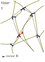
(a)

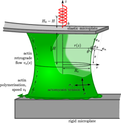
(b)

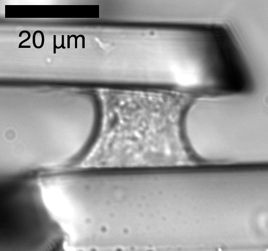
(c)

Figure 1: Model of the actomyosin behaviour and experimental setup. (1(a)) Sketch of a transiently crosslinked actin network with myosin bipolar filaments. Unbinding of a crosslinker releases elastic tension locally, the crosslinker will re-bind to the network, preserving its elastic properties, but after this loss of stored elastic energy. Myosin power-strokes have the effect of modifying the equilibrium length of the adjacent strands $\boldsymbol{{R}}$, this results in an increase of the tension (see Supplementary Discussion S2). (1(b)) Model of the mechanical components of the cell and microplate system. Microplates impose that the vertical force equilibrating the cortical tension is linked to the cell half-height $h$ with $F=2k(h_{0}-h)$. Tension along the actomyosin cortex (green surface) is anisotropic and has values $\sigma$ and $\sigma_{\perp}$ along directions $\boldsymbol{{e}}_{s}$ and $\boldsymbol{{e}}_{\phi}$. Actin treadmilling provides a boundary condition at the cell leading edge, the actin cortex undergoes a retrograde flow away from the plates. (1(c)) Transmission image of a cell and setup.

Results

Intrinsic rigidity sensing of actomyosin

The actin cortex of nonmuscle cells is a disordered network situated at the cell periphery. Actin filaments are crosslinked by proteins such as $\alpha$-actinin, however these crosslinkers experience a rapid turnover, of order $10$ s e.g. for $\alpha$-actinin [23], and actin itself has a scarcely longer turnover time [24]. The actin network is thus only transiently crosslinked. Following [20], we describe the behaviour of such a network by a rubber-like model. Up to the first order, this model leads to a stress-strain relationship of a Maxwell viscoelastic liquid in which the relaxation time is a characteristic unbinding time $\tau_{\alpha}$,

$$\tau_{\alpha}\stackrel{{\scriptstyle\triangledown}}{{\boldsymbol{\sigma}}}+\boldsymbol{\sigma}-2\tau_{\alpha}E\dot{\boldsymbol{{{{\varepsilon}}}}}=\boldsymbol{{0}},$$ (1)

where $\dot{\boldsymbol{{{{\varepsilon}}}}}$ is the rate-of-strain tensor and $\stackrel{{\scriptstyle\triangledown}}{{\boldsymbol{\sigma}}}$ the objective time-derivative of the stress tensor $\boldsymbol{\sigma}$, see Appendix S2. In the linear setting, $\boldsymbol{\sigma}=2E(\beta^{2}\left<\boldsymbol{{R}}\boldsymbol{{R}}\right>-\boldsymbol{I})$, where $E$ is the elastic modulus of the crosslinked actin network, $\beta$ is inversely proportional to the Kuhn length, and $\boldsymbol{{R}}$ is a basic element of this network, namely the strand vector spanning the distance between any two consecutive actin–actin bonds, Fig. 1(a). As long as these two bonds hold (for times much shorter than $\tau_{\alpha}$), this basic element behaves elastically, and the stress tensor $\boldsymbol{\sigma}$ grows in proportion with the strain. When a crosslinker unbinds, the filaments can slide somewhat relative to one another, and the elastic tension that was maintained via this crosslinker is relaxed: this corresponds to an effective friction, and happens at a typical rate $1/\tau_{\alpha}$. In sum, the actin network behaves like an elastic solid of modulus $E$ over a time shorter than $\tau_{\alpha}$, as crosslinkers remain in place during such a solicitation, and it has a viscous-like response for longer times with an effective viscosity $\tau_{\alpha}E$, since the network yields as crosslinkers unbind.

Such a viscoelastic liquid is unable to resist mechanical stresses [25]. However living cells are able to generate stress themselves [26] thanks to myosin bipolar filaments, which act as actin crosslinkers but are in addition able to move by one step length along one of the filaments they are bound to, using biochemical energy. Let us call $\alpha_{\text{myo}}$ the fraction of crosslinkers which are myosin filaments, and effectuate a power-stroke of step length $\ell$ at frequency $1/\tau_{\text{myo}}$. The power-stroke corresponds to a change of the binding location of the myosin head along the actin filament, and thus affects the length of the neighbouring strands $\boldsymbol{{R}}$, Fig. 1(a). Supplementary Eq. 4 includes the additional term that describes this myosin-driven evolution of the network configuration. When this equation is integrated to give the local macroscopic stress tensor $\boldsymbol{\sigma}$, this term results in a contractile stress $\boldsymbol{\Sigma}$ proportional to ${\tau_{\alpha}}E\alpha_{\text{myo}}(\ell\beta)^{2}/{\tau_{\text{myo}}}$ (see Appendix S2):

$$\tau_{\alpha}\stackrel{{\scriptstyle\triangledown}}{{\boldsymbol{\sigma}}}+\boldsymbol{\sigma}-2\tau_{\alpha}E\dot{\boldsymbol{{{{\varepsilon}}}}}=\boldsymbol{\Sigma}.$$ (2)

The three-parameter model obtained ($\tau_{\alpha}$, $E$, $\boldsymbol{\Sigma}$) is in line with early continuum models [27] and the active gel theory [28], however we do not supplement this active stress with an elastic stress, unlike previous models of mechanosensitive active gels [19, 16] where cells are treated as viscoelastic solids (Appendix S4). The interpretation of this equation is that the contractile stress $\boldsymbol{\Sigma}$ gives rise either to the build-up of a contractile tension $\boldsymbol{\sigma}$ (if clamped boundary conditions allow no strain) or a contractile strain rate $\boldsymbol{\Sigma}/(2\tau_{\alpha}E)$ (if free boundary conditions allow strain but not tension build-up, this is e.g. the case of super-precipitation in vitro [29]), or a combination of these.

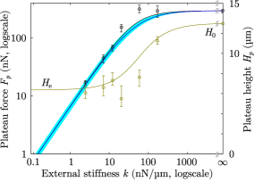
(a)

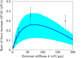
(b)

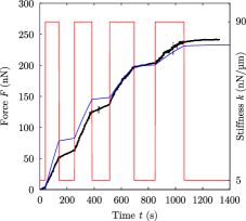
(c)

Figure 2: Predictive modelling of the stiffness-dependent cell mechanical response. (2(a)) The force and cell height at equilibrium are adapted to the stiffness of the environment up to a maximum force at high stiffness, and, for vanishing stiffness, there is a well defined equilibrium length $H_{e}$ (independent of microtubules, see Fig. S3). Circles, experimental results [13] for force (black) and height (green), black line, force predicted by the 3D model, green line, height predicted by the 3D model, blue curve and shaded area, force and confidence interval in the 1D model. Two out of the four parameters of the model adjusted in this plot, using the force at infinite stiffness and the height at zero stiffness. (2(b)) During the transient part of the experiment, the rate of loading of the cell is adapted to the stiffness of the environment. Boxes, experimental results [13], green curve and shaded area, force and confidence interval in the 1D model. One parameter of the model is fitted in this plot, the last one is adjusted on figure 4(a). (2(c)) Instantaneous adaptation to a change of the microplate stiffness $k$. Red line, stiffness imposed using a feedback loop, black dots, force measured [30], blue line, 1D model prediction of force, using the stiffness changes imposed in the experiment (red line), and the four parameters obtained in (2(a)) and (2(b)), without any further adjustment.

We then asked whether this simple rheological law for the actomyosin cortex could explain the behaviour of cells in our microplate experiments, Fig. 1(c). To do so, we investigated the equilibrium shape and force of a thin actomyosin cortex surrounding a liquid (the cytosol), in the three-dimensional geometry of the experimental setup in Fig. 1(b), Appendix S5. Surprisingly, the rigidity sensing property of cells is adequately recovered by this simple model: while a fixed maximum force is predicted above a certain critical stiffness $k_{c}=\Sigma S/H_{0}$ of the microplates, the actomyosin-generated force is proportional to $k<k_{c}$, Fig. 2(a). Here $H_{0}$ is the initial plate separation and $S$ is the section area of the actin network. Thus the contractile activity of myosin motors is enough to endow the viscoelastic liquid-like actin cortex with the spring-like response to the rigidity of its environment [31, 13], a property which was introduced phenomenologically in previous models [18]. In order to get a clear understanding of the mechanism through which this was possible, we simplified the geometry to a one-dimensional problem (Fig. 3(a)) and found that the spring-like behaviour of the contractile fluid was retained, Fig. 3(c) and Appendix S3. Indeed, for an environment (external spring) of stiffness $k$ beyond the critical value $k_{c}$, the contractile fluid is unable to strain beyond some plate deflection smaller than $H_{0}$, and equilibrium is reached as it exerts its maximal contractility $\Sigma$. For an external stiffness $k$ below the critical value, the tension $\sigma$ which is balanced by microplate force is smaller than $\Sigma$ for any admissible deflection. Thus there is a nonzero rate of contraction, $\dot{{{\varepsilon}}}<0$, as long as a maximal deflection is not reached, which is $H_{0}$ with the hypotheses done so far. The next section discusses actin polymerisation as limiting this deflection, thus setting an equilibrium cell size.

The force finally achieved is proportional to $k$ — just as a prestretched spring of stiffness $k_{c}$ would do (Fig. 3(b)), or, alternatively, just as cells do when exhibiting a mechanosensitive behaviour [18, 16] (Appendix S4). This is supported by our previous report [30] that, when the external spring stiffness is instantaneously changed in experiments, cells adapt their rate of force build-up $\mathrm{d}{F}/\mathrm{d}{t}$ to the new conditions within $0.1$ s. This observation was repeated using an AFM-based technique [14]. In [15], an overshoot of the rate adaptation, which relaxed to a long-term rate within $10$ s, was noted in addition to the initial instantaneous change of slope. While this instantaneity at the cell scale is not explained by mechanochemical regulation, this behaviour is fully accounted by the mechanical model proposed here (see Appendix S3.4, Fig. 2(b),2(c)). Thus, the actomyosin cortex is mechanosensitive by essence: its peculiar active viscoelastic nature, which arises from collective effects, provides a built-in system of adaptation to changes of the mechanical environment.

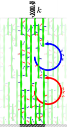
(a)

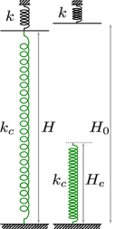
(b)

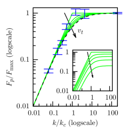
(c)

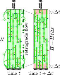
(d)

Figure 3: A one-dimensional simplification of the 3D-model preserves the essential mechanisms and results. (3(a)) Sketch of the one-dimensional model, crosslinkers and myosin unbind and rebind so that the bulk properties are constant. (3(b)) Spring model used elsewhere in the literature and to which the present model is compared. (3(c)) Equilibrium state of models and cells as a function of microplate stiffness $k$, normalised by critical stiffness $k_{c}$ and maximum force $F_{\mathop{max}\displaylimits}$ in each case. Dashes: tension of the spring model, green: tension calculated in the 1D model for different values of the speed of treadmilling $v_{\mathrm{t}}$, blue: experimental results plotted with $k_{c}=\Sigma/(H_{0}+4\tau_{\alpha}v_{\mathrm{t}})=41$ nN/$\mathrm{\upmu m}$ (no adjustment, see Supplementary Discussion S3.5). The stiffness-dependence of force in experiments is well-matched both by the spring model and the 1D model. Insert, tension calculated in the 1D model for different values of the speed of treadmilling $v_{\mathrm{t}}$, normalised by $F_{\mathop{max}\displaylimits}$ in the absence of treadmilling, $v_{\mathrm{t}}=0$: treadmilling reduces the force transmitted to the microplates. (3(d)) A dynamic equilibrium is attained when the retrograde flow exactly balances the speed of polymerisation at the boundaries, here sketched in the 1D model geometry.

Force-dependent regulation of cell size

In microplate experiments, cells are observed to spread laterally simultaneously as they deflect microplates. These two processes both affect the arc distance between the cell adhesions on each plate (Fig. S1). Cell spreading is known to be mediated by actin treadmilling [32, 33], which controls the extension of the lamellipodium [34]. An effect of treadmilling is that there is a net flow of filamentous actin from the lamellipodial region into the proximal part of the actomyosin cytoskeleton, between adhesions [35, 33], which persists even if the cell and its adhesions are immobile [17]. Thus the size of the cell is regulated by the combination of the myosin-driven contraction rate $-\dot{{{\varepsilon}}}$ of the cytoskeleton (the retrograde flow described above) and the speed $v_{\mathrm{t}}$ at which newly polymerised actin is incorporated into the cortex. This feature can be included in the model as a boundary condition, prescribing a difference $v_{\mathrm{t}}$ between the speed of the cell edge and the one of the actin cortex close to the edge (Appendix S3.2 and S5). We find that this reduces the maximum tension that the actomyosin network can develop, however the shape of the dependence versus the external stiffness $k$ is little altered (Fig. 3(c)). In particular, the force continues to be linearly dependent on $k$ for low stiffnesses, albeit with a reduced slope: this is a direct consequence of a mechanical regulation of cell height, which maintains the microplate deflection $H_{0}-H_{e}$ when $k$ varies, thus $F=k(H_{0}-H_{e})$ varies linearly with $k$ in this range.

Indeed, the equilibrium height of the cell is obtained in the classical situation when the polymerisation of actin at the cell edge is in balance with the retrograde flow which drives the actomyosin away from the cell edge (Fig. 3(d)). However, the interpretation here is not that polymerisation generates this flow, but that myosin contraction is at its origin, and that the equilibrium height is reached when the force balance between myosin contraction and external forces acting on the cell is such that retrograde flow exactly balances polymerisation speed. In the case when they do not balance, the cell edge will move at a speed which is the difference between the speed of polymerisation and the retrograde flow at the edge, until equilibrium is reached. In the case of our set-up, it is found that retrograde flow is initially faster than polymerisation, leading to a decrease of cell height, and, because of the resistance of the microplates to cell contraction, the tension $\sigma$ increases. In turn, this higher tension reduces the retrograde flow until it is exactly equal and opposite to the polymerisation speed. Treadmilling and myosin contraction thus work against one another, as has been noted for a long time [32] and is specifically described by Rossier et al. [17].

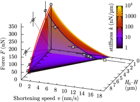
(a)

(b)

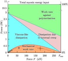
(c)

Figure 4: Liquid-like motor properties of cells. (4(a)) The rheological model leads to a Hill-type equation (3) which matches quantitatively the experimental data both during loading (blue curve at $H_{0}-H=1\mathrm{\upmu m}$: force-velocity in 1D model, boxes: experiments) and at equilibrium (surface intercept with $v=0$: 1D model, red curve: 3D model, circles: experiments). Dotted lines correspond to the force-distance relationship imposed by a given microplate stiffness $k$. Same parameters used as in Fig. 2. (4(b)) Sketch of (4(a)). (4(c)) Power usage in a microplate experiment as a function of the external load $F$: only a small part of the load-independent myosin power is being transmitted to the cell environment as mechanical power, the rest is dissipated internally or compensates the antagonistic role of polymerisation. Boxes, experimental results, to be compared to the dashed line, mechanical power at $H_{0}-H=1\tmspace+{.1667em}\mathrm{\upmu m}$, solid lines correspond to $H=H_{0}$. Same parameters used as in Fig. 2.

These phenomena regulate cell size. For low external force, myosin-driven retrograde flow is high as the tension that opposes it is small, and the balance between retrograde flow and polymerisation speed is obtained when the cell has significantly reduced its height, $H_{e}$ in Fig. 2(a). This height $H_{e}$ is thus a trade-off between the speed at which actin treadmilling produces new cortex $v_{\mathrm{t}}$ (Appendix S3) and the rate of myosin-generated contractile strain $1/\tau_{\rm c}=\Sigma/(2\tau_{\alpha}E)=\alpha_{\text{myo}}(\ell\beta)^{2}/(2\tau_{\text{myo}})$, which is itself the result of the frictional resistance of crosslinkers to myosin contraction. Indeed, in the one-dimensional toy problem, the equilibrium height of the system is $2\tau_{\rm c}v_{\mathrm{t}}$ for $k\ll k_{c}$, and thus the force developed by the external spring is $F=k(H_{0}-2\tau_{\rm c}v_{\mathrm{t}})$. In the three-dimensional full model of the cell cortex, this equilibrium height is slightly modified as a function of its geometry, but is still proportional to the product $\tau_{\rm c}v_{\mathrm{t}}$ (Appendix S5.3). This equilibrium height is reached when the treadmilling speed balances exactly the speed at which myosin in the bulk contracts the boundaries of the existing cortex, via a retrograde flow that involves the whole of the cortex but is maximum in distal regions (Fig. 3(d)). This type of competition between the protrusive contribution of actin polymerisation and the contractile contribution of myosin is of course noted in crawling cells [36], it is also observed in immobile cells where centripetal movement of actin monomers within filaments is noted even when adhesive structures are limited to a fixed location on a micropattern [17]. Thus, the cell-scale model and experiments allow to determine the speed of treadmilling, which is a molecular-scale quantity. We find $v_{\mathrm{t}}=6.5\pm 1.5$ nm/s in the 1D model, and $4$ nm/s for the 3D model, values which are in agreement with the literature [17], $4.3\pm 1.2$ nm/s. The 1D model also allows to obtain the relaxation time of the crosslinked actomyosin network, $\tau_{\alpha}=1186\pm 258$ s, consistent with elastic-like behaviour for frequencies higher than $10^{-3}$ Hz, the contractile characteristic time $\tau_{\rm c}=521\pm 57$ s, consistent with a $24$-minute completion of actin super-precipitation [29] and $\Sigma S=(2.0\pm 0.9)\cdot 10^{3}$ nN, see Appendix S3.6. These values fit both the plateau ($v=0$) force vs. stiffness experimental results, Fig. 2(a) and the dynamics of the experiments, Fig. 2(b). Without further adjustment, they also allow to predict the dynamical adaptation of the loading rate of a cell between microplates of variable stiffness [30], Fig. 2(c), and to plot the force–velocity–height phase-portrait of the experiments, Fig. 4(a).

From an energetic point of view, it may seem very inefficient to use up energy for these two active phenomena that counterbalance one another. However, in a great number of physiological functions such as cytokinesis and motility, either or both of actin polymerisation and myosin contraction are crucial. It is therefore highly interesting that, combined together, they provide a spring-like behaviour to the cell while preserving its fluid nature, endowing it with the same resilience to sudden mechanical aggression as the passive mechanisms developed by some organisms, such as urinary-tract bacteria [37] and insects [38].

Single cells have similar energetic expenses to muscles

These antagonistic behaviours of polymerisation and myosin contractility entail energy losses, which define a range of force and velocity over which the actomyosin cytoskeleton is effective. The study of the energetic efficiency of animal muscle contraction was pioneered by A. V. Hill [39], who determined a law relating force $F$ and speed of shortening $v$: $(F+a)(v+b)=c,$ where $a$, $b$ and $c$ are numerical values which depend on two values specific of a given muscle, namely a maximum force and a maximum speed, and a universal empirical constant. Hill’s law was then explained using a model based on the muscle molecular structure by A. F. Huxley [21]. Recently, we have shown that a law of the same form describes the shortening and force generation of cells in the present setup [13]. In particular, the maximum attainable force and velocity are due to energy losses. The model can shed light on the molecular origin of these losses, and leads to the quantitative force-velocity diagrams in Fig. 4(a),4(b). Indeed, in terms of $F$ and $v$, Eq. 2 yields (Appendix S3.5): $\displaystyle\left(\frac{F}{S}+E\right)\left(v+2v_{\mathrm{t}}+v_{\alpha}\right)$ $\displaystyle=(\Sigma+E)v_{\alpha}-\frac{H\dot{F}}{2S}.$ (3) Here $v_{\alpha}=H/(2\tau_{\alpha})$ interprets an internal creep velocity. The right-hand side corresponds to the source of power (minus the internal elastic energy storage term $H\dot{F}/2$), the left-hand side is the power usage (up to a constant, $Ev_{\alpha}$, added to both sides). The formal similarity of this law with Hill’s law for muscles is not a surprise when one compares the present model with Huxley’s model of striated muscle contraction. Indeed, the main components in both models are an elastic structure with transient attachments and an ATP-fuelled ‘pre-stretch’ of the basic elements of the systems which, upon release, generates either tension or contraction, or a combination of the two. Treadmilling $v_{\mathrm{t}}$ in our model superimposes an effect similar to the ones already present. It is easiest to understand this law in the extreme cases of zero speed or zero load, which correspond respectively to maximum contractile force and maximum contraction speed.

The case of zero load, $F=0$, corresponds to the highest velocity. In the case of muscle contraction, the fastest sliding of actin relative to myosin filaments is limited in Huxley’s model by the rate at which myosin heads detach after their stroke. This is because myosin heads which remain bound to actin will get entrained and exert an opposing force to the motion. This transient resistance is similar to friction. In our nonmuscle actomyosin model, crosslinkers also need to unbind so that the actomyosin network, which is elastic at short times, fluidises and flows. The velocity it reaches is thus a decreasing function of the relaxation time $\tau_{\alpha}$.

Zero speed, $v=0$, corresponds to microplates of infinite stiffness. If in addition protrusion via actin treadmilling is blocked, $v_{\mathrm{t}}=0$, there is no net deformation of the network (or sliding of the filaments in Huxley’s model), however energy is still being dissipated: indeed, myosin motors will still perform power strokes and generate tension in the network, but nearby crosslinkers and myosins themselves will also detach at the rate $1/\tau_{\alpha}$. This detachment will result in the local loss of the elastic energy that had been stored as tension of the network without resulting in a global deformation, corresponding to some internal creep. This time, the maximum force is an increasing function of relaxation time $\tau_{\alpha}$. In nonmuscle cells, actin treadmilling is still present when the cell edge is immobile [17], and reduces the maximum force that can be attained, because part of the myosin power will be used to contract this newly formed cortex.

In the intermediate regimes where neither $F$ nor $v$ are zero, the term $Fv$ corresponds to an actual mechanical work performed against the external load, Fig. 4(c). This work uses up the part of myosin energy that is not dissipated by internal creep, by effective friction or by working against the actin-driven edge protrusion.

Discussion

The model described here is based on a simple description of collective dynamics of actin and myosin that is consistent with observations at the protein scale [17], but does not include molecular sensitivity of the dynamics or actively driven reorganisation of the actomyosin cortex. We find that the linear rheological law that arises from this description allows to predict accurately the rigidity sensing experiments that we carry over two decades of external rigidity. The dynamics of cell pulling are also recovered, and we show that their similarity with the dynamics of muscle contraction [39] are due to the parallelism that exists between actomyosin dynamics in nonmuscle cells and the dynamics of thin and thick filaments in muscle [21]. Because the model is based on the collective dynamics of myosin and actin filaments, it allows to understand their role in rigidity sensing: myosin provides a contractile stress $\Sigma$ which will in turn generate traction forces at the cell–substrate contact area. In cases when $\Sigma$ is in excess to these traction forces (which resist cell contraction), a retrograde flow is generated, the cell contracts and deforms its environment. This retrograde flow is limited by the time needed by the actin network to fluidise (viscoelastic relaxation time $\tau_{\alpha}$), and is force-dependent. Retrograde flow also works against actin protrusion at the cell edge: we hypothesise that this antagonism regulates cell shape, and show in the case of our parallel microplates setup that this regulation of cell height determines the rigidity sensing features of cells. The existence of a deformation set-point had already been speculated on micropillar array experiments [31] and used as a hypothesis in modelling work [18], here we shed light on its relationship with molecular processes and retrograde flow. Because the deformation set-point is obtained as a balance between protrusion and contraction, it is versatile and is likely to be tuned by the many pathways known to affect either of these. Undoubtedly, it is a loss of energy for the cell to have such antagonistic mechanisms, which we quantify in Fig. 4(c). However, the total power of myosin action that we calculate for a single cell is of the order of $10$ fW, which is less than one thousandth of the total power involved in cell metabolism [40]. It is thus not surprising that this energy expense is not optimised in nonmuscle cells, as the evolutionary pressure on this cost can be deemed very low, while on the other hand the same structure confers to the cell its mechanical versatility and reactivity to abrupt mechanical challenges. In this, the cell may be likened to a wrestler ready to face a sudden struggle: the wrestler maintains a high muscle tone, having his own muscles work against one another. Maintaining this muscular tone is an expense of energy, but the benefit of resisting assaults widely exceeds this cost.

Materials and methods

Cell culture, fibronectin coating and drugs

Rat embryonic fibroblasts-52 (Ref52) line with YFP-paxillin, kindly provided by A. Bershadsky, Weizmann Institute, and C2-7 myogenic cell line, a subclone of the C2 line derived from the skeletal muscle of adult CH3 mice, kindly provided by D. Paulin and Z. Xue, Université Paris-Diderot, were cultured and prepared both using the procedure described in [13]. Glass microplates and, in the case of the experiment shown in Fig. 1(b), the glass coverslip at the bottom of the chamber were coated with $5\upmu$g/mL as described in [13]. In experiments described in Appendix S1 and Fig. S3, 1 $\upmu$M Colchicin was used.

Side-view experimental procedure

Ref52 or C2-7 cells were used in microplate experiments as described in [30] with the same equipment and reagents. Cells were then suspended in a temperature-controlled manipulation chamber filled with culture medium and fibronectin-coated microplates were brought in contact with a single cell as described in [13]. After a few seconds, the two microplates were simultaneously and smoothly lifted to 60 $\mathrm{\upmu m}$ from the chamber’s bottom to get the desired configuration of one cell adherent between two parallel plates. One of the plates was rigid, and the other could be used as a nanonewton force sensor [41]. By using flexible microplates of different stiffness values, we were able to characterise the effect of rigidity on force generation up to a stiffness of about $200$ nN/$\mathrm{\upmu m}$. In order to measure forces at an even higher stiffness, we used a flexible microplate of stiffness $\simeq 10$ nN/$\mathrm{\upmu m}$ but controlled the plate–to–plate distance using a feedback loop, maintaining it constant regardless of cell force and plate deflection [41, 30]. Concurrently, we visualised cell spreading under brightlight illumination at an angle perpendicular to the plane defined by the main axis of the two microplates. For conditions referred to as ‘low stiffness’, such experiments with $n=5$ Ref52 cells and $n=4$ C2-7 cells were analysed. For conditions referred to as ‘infinite stiffness’, again $n=5$ Ref52 cells and $n=4$ C2-7 cells were analysed. In both cases, the distribution of values obtained for the different cell types was not significantly different, see Fig. S4.

Bottom-view experimental procedure

Additionally, $n=4$ Ref52 cells were used in experiments using another experimental procedure allowing to image the adhesion complexes at one of the plates. The objective of the TIRF-equipped microscope (Olympus IX-71, with $488$ nm wavelength laser) was put in contact with the fibronectin-coated rigid glass plate at the bottom of the chamber. A fibronectin-coated flexible plate is put in contact with the cell after sedimentation. The deflection of the flexible plate is measured by imaging its tip with a custom-made microscope. The latter is composed of a computer-controlled light source, an optical tube (InfinitubeStandard, EdmundOptics), a long working-distance objective (20X, Mitutoyo), a prism which orients the beam in the direction of the flexible plate tip, and, eventually, a mirror that reflects back light towards the prism. Thus the flexible plate tip is imaged, through the objective and the optical tube, on a photo-sensitive detector (S3931, Hamamatsu). A feedback procedure is applied as in [13] in order to mimic an infinite stiffness of the flexible microplate.

Image analysis and geometric reconstruction

Images were treated with ImageJ software (National Institutes of Health, Bethesda, MD). For side-view experiments, 6 geometrical points were identified at each time position, corresponding to the 4 contact points of the cell surface with the microplates and to the 2 extremities of the cell ‘equator’, i.e. the mid-points where cell surface is perpendicular to microplates. Assuming a symmetry of revolution, these points define uniquely the cell equatorial radius $R_{c}$, the average radius at the plates $R_{p}$, the cell half-height $h$, and the average curvature of the cell surface $\kappa$ (average of the inverse of the radii of the circles shown in Fig. 1(a)). For bottom-view experiments, only the radius $R_{p}$ at the bottom plate can be acquired dynamically. The initial radius of cells when still spherical was measured using transmission image microscopy, it was used as the value $h_{0}$ and was found to be consistent with side-view measurements of $h_{0}$. In the case of infinite stiffness, we assumed that the curvature of fully spread cells viewed from the bottom behaved as the curvature of side-viewed cells, $\kappa h_{0}=0.90\pm 0.03$ ($n=9$). This allowed to estimate the fully-spread radius at the equator, $R_{c}$, and to use $n=13$ experiments for identifying data in the fully spread configuration for infinite stiffness.

Data analysis and model resolution

Microplate deflection time series were converted to force time series as described in [30]. Force data was then re-gridded onto the time positions of the microscopy images using the in-house open-source software DataMerge, based on the LOESS implementation of the GNU Scientific Library. Analytical calculations were assisted by the open-source computer algebra system Maxima. Numerical simulations of ordinary differential equations derived from the model were simulated using the GNU Octave scientific computing programming language for figure 2. Analytical implicit equations were plotted using the open-source Gnuplot software in figures 2(a), 3(c) and 4(a).

Acknowledgments

J.E. thanks especially John Hinch, Claude Verdier, Martial Balland, Karin John, Philippe Marmottant and Cyril Picard for fruitful discussions. J.E. wishes to acknowledge funding by Région Rhône-Alpes (Complex systems institute IXXI and Cible), ANR ”Transmig” and Tec21 (Investissements d’Avenir - grant agreement n° ANR-11-LABX-0030). The experimental work was supported in part by ANR funding (ANR-12-BSV5-0007-01, ”ImmunoMeca”).

Appendix

S1 Role of microtubules

It has been reported that in addition to the substrate, part (of order 13%) of the cortical tension could be balanced by the resistance to compression of microtubules [1]. We have thus controlled whether this was the case in our setup, in particular for low external stiffness, which corresponds to lower height of cells and thus are geometrically more likely to involve microtubule compression. The results, shown in Fig. S3, indicate that there is no such influence within experimental error. This allows us to neglect the role of microtubules compared to actomyosin tension and microplate resistance to bending in the modelling that follows.

S2 Model derivation

As stated in the text of the article, we are looking for the simplest model consistent with the fact that the actin plus crosslinkers network in vivo is not able to resist extensional stress in the long term. This is consistent with a dominant loss modulus at low frequencies in cell-scale rheological probing [2] and in vitro studies [29], and is linked with the fact that crosslinkers in vivo are transient with a short residence time [24]. Basic models of transiently crosslinked networks based on rubber-like models were first explored by Green and Tobolsky [3] and Yamamoto [20], and their nonlinear properties are still being investigated [4]. Their response, up to the first order, turns out to be the same as the one of polymer solutions, that is, their stress-strain relationship is governed by Maxwell constitutive Eq. 1,

$$\tau_{\alpha}\stackrel{{\scriptstyle\triangledown}}{{\boldsymbol{\sigma}}}+\boldsymbol{\sigma}-2\tau_{\alpha}E\dot{\boldsymbol{{{{\varepsilon}}}}}=0,$$

with ${\boldsymbol{\sigma}}=2E\left(\beta^{2}\left\langle\boldsymbol{{R}}\boldsymbol{{R}}\right\rangle-\boldsymbol{I}\right)$ ([5, p. 116], the parameter $\beta^{2}=3/(2N_{K}b_{K}^{2})$ is related to $b_{K}$ the length and $N_{K}$ the number of Kuhn steps between two crosslinks). Here the upper convected Maxwell tensor derivative $\stackrel{{\scriptstyle\triangledown}}{{\boldsymbol{\sigma}}}=\dot{\boldsymbol{\sigma}}-\boldsymbol{{\nabla}}\boldsymbol{{v}}^{\mathrm{T}}\boldsymbol{\sigma}-\boldsymbol{\sigma}\boldsymbol{{\nabla}}\boldsymbol{{v}}$ takes into account the affine stretching of the strand vectors $\boldsymbol{{R}}$, the basic units of the network, by the velocity gradient $\boldsymbol{{\nabla}}\boldsymbol{{v}}$. The difference is that, for polymer solutions, the time $\tau_{\alpha}$ is the ratio of solvent viscosity to polymer elasticity, because this is the characteristic time at which the polymers can deform relatively to an affine global deformation of their surroundings (the solvent, [5, p. 123]), while, in the case of transiently crosslinked networks, $\tau_{\alpha}$ is the characteristic unbinding time of the crosslinks. Thus, the product $\tau_{\alpha}E$ which has the dimension of a viscosity is only some apparent viscosity at the macroscopic scale, and corresponds in fact to an elastic energy dissipation at rate $1/\tau_{\alpha}$. If there is a large number of crosslinkers present along a single filament, there will not be a single relaxation time $\tau_{\alpha}$ but several [6]. In the present work, we choose to investigate the properties of the single-relaxation time model above because this allows to calculate analytically the model solution while retaining the essence of a long-time viscous-like and short-time elastic-like material.

A fraction $\alpha_{\text{myo}}$ of the crosslinkers considered are myosin bipolar filaments. In addition to their crosslinking role, they may effectuate a power-stroke at a frequency $1/\tau_{\text{myo}}$, which results in “sliding” the corresponding crosslinker by the myosin step length $\ell$. If $\psi(\boldsymbol{{\rho}})$ is the orientational distribution function [5], this appears as additional sink and source terms in the right hand side of the probability balance equation,

$$\frac{\partial\psi}{\partial t} +\nabla_{\boldsymbol{{\rho}}}\cdot\left(\dot{\boldsymbol{{R}}}\psi\right)$$

$$=\frac{\alpha_{\text{myo}}}{\tau_{\text{myo}}}\left(-\psi(\boldsymbol{{\rho}})+\frac{1}{2}\psi(\boldsymbol{{\rho}}-\ell\boldsymbol{{\rho}}/|\boldsymbol{{\rho}}|)+\frac{1}{2}\psi(\boldsymbol{{\rho}}+\ell\boldsymbol{{\rho}}/|\boldsymbol{{\rho}}|)\right)$$

$$\simeq\frac{\alpha_{\text{myo}}\ell^{2}}{2\tau_{\text{myo}}}\frac{\partial^{2}\psi}{\partial|\boldsymbol{{\rho}}|^{2}}$$ (4)

which, multiplied by $\boldsymbol{{\rho}}\boldsymbol{{\rho}}$ and integrated over all configurations, yields an additional term of contractility

$$\tau_{\alpha}\stackrel{{\scriptstyle\triangledown}}{{\boldsymbol{\sigma}}}+\boldsymbol{\sigma}-2\tau_{\alpha}E\dot{\boldsymbol{{{{\varepsilon}}}}}=\boldsymbol{\Sigma}=\Sigma\boldsymbol{A},$$

where $\Sigma=E\frac{\tau_{\alpha}}{\tau_{\text{myo}}}{\alpha_{\text{myo}}(\ell\beta)^{2}}$ is proportional to the myosin concentration and power-stroke frequency. The tensor $\boldsymbol{A}$ is the local orientation tensor of the actin fibres,

$$\boldsymbol{A}=\int_{\boldsymbol{{\rho}}}\frac{\boldsymbol{{\rho}}\boldsymbol{{\rho}}}{|\boldsymbol{{\rho}}|^{2}}\psi\,\mathrm{d}\boldsymbol{{\rho}}.$$

The ratio of the apparent viscosity $\tau_{\alpha}E$ and contractile stress $\Sigma$ provides us with another characteristic time, $\tau_{\rm c}=2\tau_{\alpha}E/\Sigma=2\tau_{\text{myo}}\alpha_{\text{myo}}^{-1}(\ell\beta)^{-2}$, which characterises the dynamics of shrinking of an actomyosin network in the absence of crosslinkers, as is the case in in vitro experiments [29].

Note that both characteristic times of crosslinker unbinding $\tau_{\alpha}$ and of myosin power-stroke $\tau_{\text{myo}}$ have been taken as constants, independent of the stress or strain they are submitted to. It is of course well established that there is a dependence of these parameters on stress and strain [7], which would introduce a nonlinearity in the model. An important, unsolved question is to determine whether these dependences are or not major players in the cell-scale mechanical behaviour of actomyosin, e.g. through a stress-driven ripping of crosslinks. As their effect is a nonlinear variation of the above model, the standard modelling procedure is to study the linear response first (with constant characteristics times), before considering the full nonlinear model. It is found in the sequel that the linear model is sufficient to reproduce the experimental data, that is, for our experiments, collective effects explain the observed behaviour by themselves. In these conditions, the effect of additional nonlinear terms could not be distinguished from this linear baseline, and were therefore not introduced in the present work.

The model obtained is thus the one of a viscoelastic liquid. This is in line with the seminal model by He and Dembo [27] who modelled the cytoskeleton as a viscous fluid and used it in numerical simulations of the cytokinesis. This is also similar to the actin dynamics part of the model used by [8] to simulate keratocyte migration. We provide above a microstructure-based derivation of this class of models, which allows us to interpret the dissipation in terms of molecular behaviours (see the discussion on Hill’s law, Appendix S3.5). This type of model, to the best of our knowledge, was never used to study mechanosensing behaviours of single cells. In the sequel (Appendix S4), we compare it to models that have been used to analyse cell-scale mechanosensing, but will first investigate its basic predictions.

S3 One-dimensional problem

S3.1 In the absence of treadmilling

In this section we investigate the behaviour of a material modelled by the constitutive law, Eq. 2, in a simplified, one-dimensional geometry described in Fig. 3(a). The actomyosin network is assumed to occupy an infinite cuboid between two horizontal plates, one of which is fixed and the vertical position of the other governed by a spring of stiffness $k/S$ (per unit area) and equilibrium distance with the other plate $H_{0}$. If the current distance between the plates is $H$, the force exerted by the top plate on the material is thus $F/S=k(H_{0}-H)/S$ per unit area.

We assume that the bulk forces acting on the actomyosin network (such as the friction with the cytosol) are negligible compared to the force developed by myosin contraction, this writes:

$$\boldsymbol{{\nabla}}\cdot\boldsymbol{\sigma}=\boldsymbol{{0}},$$ (5)

with the boundary condition $\boldsymbol{\sigma}\boldsymbol{{e}}_{z}=(F/S)\,\boldsymbol{{e}}_{z}$ at the upper plate; and corresponds to neglecting friction with the cytosolic fluid in the balance between the actomyosin stress and the force at the plates. By symmetry, only the vertical component $\sigma_{zz}$ of the stress tensor $\boldsymbol{\sigma}$ in the actomyosin material is nonzero, we denote it $\zeta$, from the above we have $\partial_{z}\zeta=0$ and thus the boundary condition imposes $\zeta=F/S=k(H_{0}-H)/S$ at every $z$, the stress is fully transmitted through the material.

On the other hand, the rate-of-strain tensor $\dot{\boldsymbol{{{{\varepsilon}}}}}$ is also limited to a vertical component $\dot{{{\varepsilon}}}=\dot{H}/H$. Using these equalities, the constitutive Eq. 2 describes the complete dynamics of the system. In particular, a permanent regime ($\dot{{{\varepsilon}}}$=0, $\dot{\zeta}=0$) is reached for

$$F_{p}=\zeta_{p}S =\frac{\Sigma S}{2}\left(\frac{k+k_{c}}{k_{c}}-\sqrt{\left(\frac{k+k_{c}}{k_{c}}\right)^{2}-\frac{4k}{k_{c}}}\right)$$

$$=\left\{\begin{array}[]{ll}kH_{0}&\text{if }k<k_{c},\\ \Sigma S&\text{else},\end{array}\right.$$ (8)

for $k<k_{c}$, with $k_{c}=\Sigma S/H_{0}$. The actomyosin model’s response is thus very close to the behaviour of a spring of stiffness $k_{c}$ and free length $0$, when put in series with an external spring of stiffness $k$: Indeed, the asymptotes are the same for $k\rightarrow 0$ and $k\rightarrow\infty$ (Fig. 3(c)), which is not obvious since in the permanent regime the model only includes viscous dissipation and contractility. We have thus shown that a contractile fluid behaves like a spring in these conditions.

Indeed, when the cell is pulling on a spring of stiffness $k$, the maximum deflection it can impose to the spring is $H_{0}$, e. g. the initial cell height and, consequently, the maximum height it can shorten. However, this maximum deflection is achieved only if the maximum force generated by the cell $\Sigma S$ is larger than the external spring force at maximum deflexion $kH_{0}$, in other words only if $k$ is lower than $k_{c}=\Sigma S/H_{0}$. In that case, the force reached is $kH_{0}$, thus proportional to $k$. In the other case $k>k_{c}$, the deflection is less than $H_{0}$ and is set by having an equal tension $\Sigma S$ in both the external equivalent spring $k$ and the cell.

S3.2 In the presence of treadmilling

We now introduce the fact that actin filaments in vivo are constantly being polymerised from one end (‘plus’ end) and depolymerised, mostly from the other (‘minus’ end), which results in the so-called treadmilling phenomenon [32]. Assuming that this treadmilling is at steady-state in the cell on average at the relevant time scale of our experiment, the effect of treadmilling in the bulk does not affect the modelling assumptions done in Appendix S2: the elastic modulus $E$ of the crosslinked network at any instant will have a constant average. However, at the boundary, some filaments will have their ‘plus’ end oriented towards the boundary and thus polymerisation of these will entail a net extension of the material (before stress equilibration, depending on the boundary conditions).

In the framework of our one dimensional toy problem, this introduces a drift between the deformation of the material and the displacement of the boundary, which can be expressed as:

$$\dot{H}=H\dot{{{\varepsilon}}}+2v_{\mathrm{t}}$$ (9)

with $v_{\mathrm{t}}=\ell_{\text{a}}/\tau_{\text{a}}$ the treadmilling speed, that is, the extra length added by a monomer polymerising divided by the characteristic time for an ATP-fuelled monomer addition. The factor $2$ is due to this effect taking place at both plates.

When injected into the constitutive model, this modifies the level of force (and height $H_{p}$) in the permanent regime:

$$F_{p}=\zeta_{p}S=\frac{\Sigma S}{2}\left(\frac{k+k_{c}}{k_{c}}-\sqrt{\left(\frac{k+k_{c}}{k_{c}}\right)^{2}-\frac{4k}{\Sigma S}(H_{0}-H_{e})}\right),$$ (10)

with a modified critical stiffness $k_{c}=\Sigma S/(H_{0}+H_{\alpha})$. Here $H_{\alpha}=4\tau_{\alpha}v_{\mathrm{t}}=4\tau_{\alpha}\ell_{\text{a}}/\tau_{\text{a}}$ is a characteristic elastic length of newly polymerised material. The critical stiffness $k_{c}$ is lowered in proportion with the corresponding relative increase of height. We have also introduced another new parameter, the length $H_{e}=2\tau_{\rm c}v_{\mathrm{t}}=4\frac{\tau_{\text{myo}}}{\tau_{\alpha}}\frac{\ell_{\text{a}}}{(\ell\beta)^{2}\alpha_{\text{myo}}}$. This length is discussed in the main text, it is a trade-off between the rate at which actin contracts under the effect of myosin, and the speed at which actin network expands by polymerisation at its edges. It defines the shortest height that the cell achieves in the 1D model, when the stiffness of the plates is vanishingly small: in that case, all of the work of myosins is spent in contracting the part of actin network newly polymerised.

For a low stiffness, this expression has for asymptote $F_{p}\sim k(H_{0}-H_{e})$, and for a large stiffness,

$$F_{p}\rightarrow\Sigma S\frac{H_{0}-H_{e}}{H_{0}+H_{\alpha}}$$ (11)

This does not change the qualitative spring-like response of the material, only the equilibrium length of the equivalent spring is not zero anymore but $H_{e}$. This means that as the device stiffness goes to zero, the height of the model meshwork will tend to $H_{e}=2\tau_{\rm c}v_{\mathrm{t}}$, which is a dynamic balance between the speed $2v_{\mathrm{t}}$ at which new material is added at the two boundaries (modelling polymerisation), and the rate $1/\tau_{\rm c}$ at which the existing material is contracted by the myosin motors. Inside this model material, even once the final length $H_{e}$ is reached and the boundaries are immobile, there remains a continuous centripetal flow (Fig. 1(b)) that is very reminiscent of the retrograde actin flow observed in both crawling [32] and immobile spread cells [17]. Exactly as in these cases, this is made possible by depolymerisation inside the model material. This is an additional source of energy dissipation in steady state, when the cell is apparently at equilibrium with constant length $H_{e}$ and force $F_{p}$.

S3.3 Dynamics

The above constitutive and force balance equations can be written in terms of one equation only with the tension as the unknown,

$$\frac{\partial\zeta}{\partial t}=\frac{\Sigma\left(k(H_{0}-H_{e})/S-\zeta\right)+\zeta\left(\zeta-k(H_{0}+H_{\alpha})\right)}{\tau_{\rm c}\Sigma+\tau_{\alpha}(\zeta+kH_{0}/S)}.$$ (12)

One can analyse the rate of tension increase when the system begins to pull and $\zeta$ is still much smaller than $\Sigma$, for a low stiffness $k\ll ES/H_{0}$,

$$\frac{\partial F}{\partial t}=\frac{k(H_{0}-H_{e})-F(t)}{\tau_{\rm c}}\sim\frac{F_{p}(k)-F(t)}{\tau_{\rm c}}.$$ (13)

And for high stiffness $k\gg ES/H_{0}$,

$$\frac{\partial F}{\partial t} =\frac{\Sigma S(H_{0}-H_{e})-F(t)(H_{0}+H_{\alpha)}}{\tau_{\alpha}H_{0}}$$ (14)

$$=\frac{(F_{p}(k)-F(t))\,(H_{0}+H_{\alpha})}{\tau_{\alpha}\,H_{0}}.$$ (15)

Experiments for very low values of the microplate stiffness $k$ allow to identify the parameters $\tau_{\rm c}$ and $v_{\mathrm{t}}$ of the model.

From $n=9$ experiments with $k\leq 1.6$ nN/$\mathrm{\upmu m}$, we find $2\tau_{\rm c}v_{\mathrm{t}}=H_{e}=6.6\pm 1.1\,\mathrm{\upmu m}$ and $H_{0}=13.2\pm 0.1\,\mathrm{\upmu m}$. This is consistent with the fact that $\partial F/(\partial k)=H_{0}-H_{e}=6.8\pm 0.4\,\mathrm{\upmu m}$ in [13]. Additionally, the maximum force attained $F_{p}$, the current force $F(t)$ and the rate of growth of this force ${\partial F}/{\partial t}$ allow to calculate $\tau_{\rm c}$ using Eq. 13, $\tau_{\rm c}=(F_{p}-F(t))({\partial F}/{\partial t})^{-1}=521\pm 57$ s. This yields $v_{\mathrm{t}}=6.5\pm 1.5$ nm/s, which is consistent with the literature [17] as stated in the main text.

S3.4 Response to a step-change of external stiffness

In [30], we are able to vary instantaneously (within $0.1$ s) the stiffness $k$ of the external spring, while ensuring that there is no instantaneous change of the force $F$ felt by the cell or of the microplate spacing $H$. In the modelling, this corresponds to an instantaneous change of both $k$ and $H_{0}$ at time $t^{*}$ such that $F$ and $H$ are continuous. We can thus write the following relations, ensured by the experimental setup:

$$k(t)=\left\{\begin{array}[]{l}\!k_{0}\text{, }t<t^{*},\\ \!k_{1}\text{, }t>t^{*},\end{array}\right.$$

$$\begin{array}[]{ccc}\!\!\!F(t)=F^{*}+\phi(t),&\!\!H(t)=H^{*}-\frac{\phi(t)}{k(t)},\end{array}$$

where $\phi(t)$ is the variation of force around the force at time $t^{*}$, $\phi(t^{*})=0$.

Changing only the stiffness in this manner ensures that the cell does not feel any step-change: indeed, force and geometry are preserved, the only change is the response of the microdevice to a variation of the force applied to it. The experimental result is that, despite the fact that none of the physical observables have been changed for the cell, its rate of loading ${\partial F}/{\partial t}$ of the device is instantaneously modified. In [30], it is found that, when going from a stiffness $k_{0}$ to a stiffness $k_{1}$, the new rate of loading matches the rate of loading that the same cell type exhibits in a constant stiffness $k=k_{1}$ experiment, at a time such that $F=F^{*}$. In [15], this experiment is repeated with another cell type and it is also found that the rate of loading is instantaneously changed. However, the value ${\partial F}/{\partial t}$ for $t\gtrsim t^{*}$ exhibits an overshoot: it is initially different from the value of the corresponding constant stiffness experiment, and exhibits a relaxation towards it.

We can rewrite Eq. 12 around $\zeta^{*}=F^{*}/S$, we find:

$$\frac{\partial F}{\partial t}(t^{*})=k(t)\frac{H^{*}(\Sigma S-F^{*})-H_{\alpha}F^{*}-H_{e}\Sigma S}{\tau_{\rm c}\Sigma S+\tau_{\alpha}(k(t)H^{*}+2F^{*})}.$$ (16)

The result is thus a step-function, whose value for $t\gtrsim t^{*}$ is exactly the rate of growth predicted by the model for a constant stiffness experiment with $k=k_{1}$. This corresponds to the experimental results in both [30] and [15], except for the overshoot found in the latter.

The step-change of the rate of loading can thus be explained by a purely intrinsic property of the cell’s cytoskeleton, as developed in the main text.

In [15], a model is proposed that accounts for a step-change and relaxation, as they observe experimentally. However this model has a limited validity around $t^{*}$ and breaks down at long times, predicting infinite force. Here, our model originally aiming at describing the long-time behaviour of the cell depending on stiffness predicts the main feature of the experiments (the step-change of the rate of loading), but not the overshoot found in one of the experiments. Our model however may produce this type of overshoot if more than a single relaxation time is used. This would correspond to replacing the spring $k_{1}$ in the model in [15] by our viscoelastic constitutive equation. This is found not to be necessary to explain the data studied here.

In Fig. 2(c), we give a numerical simulation result that corroborates the step-change of ${\partial F}/{\partial t}$ found in Eq. 16 and can be compared to an experimental curve without any parameter adjustment. The time-profile of the microplate effective stiffness is imposed to be the same in the numerical simulation as in the experiment. The profile of force increase obtained presents the same instantaneous change of slope as the stiffness is varied, and the overall profiles match quantitatively.

S3.5 Hill’s law

We examine the power dissipation predicted by the one-dimensional model between two boundaries. The boundaries move towards the sample at velocity $v$ (which is thus positive when the sample contracts) and feel a force $F$ exerted by the sample (positive in the direction of contraction).

Hill’s historical experiment [39] takes place at a constant level of force $F$. Our experiments, on the other hand, prescribe a relationship between $F$ and $v$ through the microplate stiffness, ${\partial F}/{\partial t}=-kv$. Both can scan the $F$–$v$ relationship by varying $F$ for the former or $k$ for the latter (in the case of [13], we needed to investigate this relationship for a fixed $H=H_{0}-\delta$ where $\delta$ is small), Fig. 4(a) and 4(b). The calculation below does not require to use either of these experimental ways to scan the $F$–$v$ relationship. It relies only on the material properties of the sample.

As above, the mechanical equilibrium of the sample imposes that the vertical component of the stress tensor $\zeta$ is equal to $F/S$. Also, the treadmilling produces a mismatch between the plate velocity $v=\dot{H}$ and the recoil of the existing network at the plate $-H\dot{{{\varepsilon}}}$, expressed by $v=-H\dot{{{\varepsilon}}}+2v_{\mathrm{t}}$ (see Eq. 9). These relations can be injected into the constitutive Eq. 2:

$$\tau_{\alpha}\left(\dot{F}-2\dot{{{\varepsilon}}}F\right)+F-2\tau_{\alpha}ES\dot{{{\varepsilon}}}=\Sigma S.$$

We recover a virtual work formulation by multiplying this by the velocity $H/(2\tau_{\alpha})$. Adding the constant $ESH/(2\tau_{\alpha})$ to both sides, this work can now be factorised in the manner of Hill’s law:

$$\left(\frac{F}{S}+E\right)\left(v+2v_{\mathrm{t}}+\frac{H}{2\tau_{\alpha}}\right) =(\Sigma+E)\frac{H}{2\tau_{\alpha}}-\frac{H}{2S}\dot{F}.$$ (17)

The meaning of some of these terms is explained in the main text.

In the case when the velocity $v$ is zero, the force generated is finite as calculated above, Eq. 11, which can also write:

$$\frac{F_{\max}}{S}=\Sigma\left(1-\frac{E+\Sigma}{\Sigma}\frac{2v_{\mathrm{t}}}{v_{\alpha}+2v_{\mathrm{t}}}\right)$$

Even if both $v$ and $v_{\mathrm{t}}$ are zero, and thus the actomyosin does not contract macroscopically ($\dot{{{\varepsilon}}}=0$), the force generated remains finite since it does work at a molecular scale. Actin polymerisation, by adding new material at the edges, introduces a ‘boundary creep’, which consumes additional work in conditions of fixed length ($v=0$).

As stated in the main text, apart from the polymerisation ‘boundary creep’, this is the same dissipative mechanism as in the model of muscle contraction by Huxley [21]. In this model, myosin ‘elastic tails’ are prestretched preferentially in one direction before binding the actin thin filament. When there is no net sliding ($v=0$), they eventually unbind without having had the opportunity to provide work, that is, they have conserved this level of stretching. Although this is not explicitly written in the 1957 paper, the prestretch that had been bestowed on the myosin ‘elastic tail’ is thus lost.

Zero force $F=0$ condition is a (theoretical) limit corresponding to zero-stiffness of the microplate. This is not attainable experimentally, as cells do not spread on both plates if their displacement does not generate any external force—which corresponds to the impossibility to apply any normal force to the plates. This effect probably has to do with the mechanism of force reinforcement of adhesions. In the model however, the limit can be studied, and yields a maximum velocity,

$$v_{\max}+2v_{\mathrm{t}}=\frac{\Sigma v_{\alpha}}{E}=\frac{H}{\tau_{\rm c}}.$$

This corresponds to the power injected by the myosin motors, divided by the elastic modulus of the crosslinked network (minus the treadmilling contribution): indeed, in this limit, the myosins work against the elasticity of the actomyosin itself. The maximum velocity is thus limited by the rate $\tau_{\alpha}$ at which the actin network fluidises thanks to the detachment of crosslinkers. In comparison to the case of muscles, actin treadmilling reduces the maximum speed of shortening by $2v_{\mathrm{t}}$, as the receding speed of the edge of the actin network must compensate for this speed of protrusion. Quantitatively, using the values obtained in Appendix S3.3, we predict $v_{\max}\simeq 12.3$ nm/s, this is very close to $v_{\max}=13$ nm/s published in [13].

Again, the dissipation here is of the same nature as for muscles in the model by Huxley: in his case, the only crosslinker between thin and thick filaments are myosin heads, and zero force is obtained at the finite velocity at which the work rate performed by pulling myosin heads is exactly balanced by the work rate needed to deform myosin heads that have not yet detached from the actin filament. They will eventually detach, thus dissipating at a fixed rate the elastic energy that has been transferred to them.

When neither $F$ nor $v$ are zero, there is a nonzero productive work performed on the plates. Because of the existence of maximum force and velocity, it is necessarily written

$$\frac{Fv}{F_{\max}v_{\max}}=r\left(1-\frac{F}{F_{\max}}-\frac{v}{v_{\max}}\right).$$

In both the experiments by A. V. Hill [39] and ours [13], $r$ is found to be mostly independent of $F$ and $v$, and $r\simeq 0.25$. In Huxley’s model of muscles, $r$ is a signature of the preferential pre-stretch of myosins that models the power-stroke, normalised by the detachment rate [21, 9]. In our model of cells, $2r\simeq\tau_{\rm c}/\tau_{\alpha}$ is the ratio of the characteristic times of contraction and of stress relaxation through crosslinker unbinding. This does not explain the coincidence of finding the same value of $r$ in both cells and muscles, however we note that this parameter has a similar signification in both models.

Specifically,

$$r =\frac{E}{\Sigma\left(1-\frac{E+\Sigma}{\Sigma}\frac{2v_{\mathrm{t}}}{v_{\alpha}+2v_{\mathrm{t}}}\right)}.$$ (18)

Thus in our case, Hill’s parameter $r$ is such that

$$\frac{E}{\Sigma}=\frac{\tau_{\rm c}}{2\tau_{\alpha}}\leq r\leq\frac{\tau_{\rm c}}{2\tau_{\alpha}}+\left(\frac{\tau_{\rm c}}{2\tau_{\alpha}}\right)^{2},$$ (19)

depending on $v_{\mathrm{t}}$.

Note that these equations can be applied to the actomyosin pushing against an obstacle, with $0\leq-F\leq ES$ and $0\leq-v\leq v_{\mathrm{t}}$.

S3.6 Quantitative analysis

Since $r\simeq 0.25$ in experiments [13], ${\tau_{\rm c}}/{\tau_{\alpha}}$ has to be in the range $0.4$ to $0.5$, thus since $\tau_{\rm c}=521\pm 57$ s, we have $\tau_{\alpha}=1186\pm 258$ s. In turn, using also $v_{\mathrm{t}}=6.5$ nm/s (see S3.3), we find $\Sigma S=F_{\max}(H_{0}+H_{\alpha})/(H_{0}-H_{e})=(2.0\pm 0.9)\cdot 10^{3}$ nN ($n=13$). Thus the four parameters of the 1D model, namely $\tau_{\alpha}$, $\tau_{\rm c}$, $v_{\mathrm{t}}$ and $\Sigma S$ are identified using only the average maximum force (equilibrium of infinite stiffness experiments), maximum velocity (dynamics of experiments with very low stiffness), and shortest height at equilibrium (experiments with very low stiffness), plus the shape of the Hill-type law (parameter $r$).

The other experimental data (stiffness-dependence of the force, Fig. 3(c); dynamics as the microplate stiffness is modified, Fig. 2(c); and values of $F(t)$ at $H_{0}-H=1\mathrm{\upmu m}$, Fig. 4(a)) are matched by the model without any adjustable parameter. E.g., the values found yield a critical stiffness $k_{c}=\Sigma S/(H_{0}+4\tau_{\alpha}v_{\mathrm{t}})=41$ nN/$\mathrm{\upmu m}$, which is consistent with the experimental results, Fig. 3(c).

Moreover, the values for $\tau_{\rm c}$, $\tau_{\alpha}$ and especially $v_{\mathrm{t}}$ are independently measurable and are consistent with the literature, see text.

S4 Comparison with other models featuring cell-scale mechanosensing

In [18, 10], the cell is modelled as a linear elastic body having an intrinsic equilibrium shape, and which is prestretched to some maximum strain, in our notation:

$$\boldsymbol{\sigma}=2E(\boldsymbol{{{{\varepsilon}}}}-\boldsymbol{{{{\varepsilon}}}}_{0}),$$

with $\boldsymbol{{{{\varepsilon}}}}_{0}$ an equilibrium shape that the cell would take in the absence of external stresses. They supplement this model with a phenomenological feedback on the elastic modulus, on the time scale of hours or days, which corresponds to the phenomenon of stress-fibre polarisation [11]. This long term effect is out of the scope of our model and experiments, thus our model compares to theirs before this feedback comes into play. In a one-dimensional setting, their model thus corresponds to the prestretched spring in Fig. 3(b), which yields a stiffness-dependence closely mimicking experimental data and our model predictions, Fig. 3(c). Our model in addition provides a microstructure basis for this qualitative behaviour and a quantitative reading of experiments, in particular the equilibrium shape $\boldsymbol{{{{\varepsilon}}}}_{0}$ and cell stiffness $k_{c}$ in [18] are explicited, respectively, as proportional to the product of a characteristic contraction time and the treadmilling speed, $\tau_{\rm c}v_{\mathrm{t}}$, and as the ratio of the myosin contractile stress and a length, $k_{c}=\Sigma S/(H_{0}+4\tau_{\alpha}v_{\mathrm{t}})$.

In [16], they introduce a model also in the framework of active gel theory. However, they resort to the stress-strain relationship of [18] so as to avoid to calculate the orientation tensor $Q_{ij}$ of the cytoskeleton and use a 1D linear elastic stress-strain relationship, their equation (S7) writes in our notation $\sigma=2E(H-H_{e})$.

In [19], they present a 1D visco-elastic solid model, combining their equations (2) and (5) writes in our notation:

$$\sigma=2E(H-H_{e})+2\eta\dot{H}.$$

with $H_{e}=l^{0}_{C}-F_{S}/k_{C}$ in their notation. To the difference to the previous models, the viscous term added in this model allows to study the dynamics of the cell shortening. However, the equilibrium shape in all three models is a static elastic balance between the environment resistance to deformation and a phenomenological internal elasticity, which corresponds to the spring model described in Fig. 3(b).

S5 Three dimensional problem

In this section, we present a full three-dimensional model of the cell mechanics as a contractile visco-elastic thin shell, obeying the rheological Eq. 2, and enclosing an incompressible cytosol. Forces are transmitted to the microplates at the contact line between the cell boundaries and the microplates.

S5.1 Geometry

It is seen from experimental observations that the cell boundaries connecting the plates are in most cases very well approximated by an arc of circle (Fig. 1(b), insert). This had already been shown in the case of cells spread on a microneedle array having reached a stationary shape [12], in the present setup we find that it is also true while the cell is spreading (Fig. 1(a)).

When observing cells from the side, we assume that the cell shape is cylindrical. This is supported by other experiments where cells are observed from the bottom in TIRF, Fig. 1(b). Thus, along the axis $z$ orthogonal to the microplates, whose location is parametrised as $z=\pm h$ where $h$ is the half-height of the cell, we can fit experimental results using the law:

$$r(z)=R_{c}+\frac{1}{\kappa}\left(1-\sqrt{1-(\kappa z)^{2}}\right),$$ (20)

where $R_{c}$ is the radius at the cell equator ($z=0$) and $\kappa$ the signed curvature in the vertical plane, Fig. 1(b). The curvature $\kappa$ evolves in time from a positive curvature ($t=10$ s in Fig. 1(a)) to a negative one ($t=120$ s and later in Fig. 1(a)).

To the physicist it may be a surprise that the cell shape is not well fitted by a minimal surface such as a catenoid. Indeed, although each boundary seen on Fig. 1(a) can be reasonably fitted with an hyperbolic cosine function, the asymptotes of these fits do not match: the cell shape is close to a “minimal” surface with a different weight on its curvatures, $\kappa\sigma+\kappa_{\perp}\sigma_{\perp}=0$, where $\kappa_{\perp}$ is the curvature in a plane orthogonal to the side view. In light of Laplace law, these weights can be interpreted as tensions of different magnitude in the longitudinal ($\boldsymbol{{e}}_{s}$ in Fig. 1(b)) and orthoradial ($\boldsymbol{{e}}_{\phi}=\boldsymbol{{e}}_{n}\times\boldsymbol{{e}}_{s}$) directions. The reason for these different tensions and details of this Laplace law are given in the next section. We cannot fit the cell shape with an analytical function matching this law, firstly because functions solving the corresponding differential equation have never been investigated and do not have the same properties as the hyperbolic cosine, secondly because the tensions $\sigma$ and $\sigma_{\perp}$ actually vary in some measure along the vertical direction.

From this we can calculate the volume of the cell through time. Here again, the physicist is surprised to find that the volume defined by Eq. 20 and the plate positions $z=\pm h$ is not a constant, Fig. S2. However, this volume is not the volume of the cell itself but the volume enclosed by the lateral cell boundaries: indeed, it is observed in side views of cells presenting such a large enclosed volume increase that the cell detaches from the microplates in the central region of the contact area (Fig. S2), forming a “pocket” between the cell membrane and the microplate, which has every reason to be filled by culture medium seeping between the adhesions seen in Fig. 1(b). Although it was not possible to track the volume of these pockets through time and compare it to the enclosed volume variations, we can estimate the energetic cost of the corresponding water flow: adhesions are more than 1 $\mu$m apart over 10 to 20 $\mu$m length between the periphery and the central region where medium pocket is being formed. Assuming a low estimate of $N>30$ passages of height 0.1 $\mu$m through which medium can flow from the periphery to the cell interior, we obtain that the pressure needed to drive the flow noted in Fig. S2 is about $10$ Pa, and that the power needed for this is of the order $10^{-17}$ W : that is, 2 orders of magnitude smaller than the actomyosin power transmitted to the microplate and measured in the experiments. The formation of such pockets is thus very plausible, and indeed is observed in most experiments when the force is large.

The data we present does not allow to check whether the totality of the change of apparent volume is due to this water seepage. Therefore, there may be also some volume variations due to a regulation of cell volume [13] superimposed to the one due to the formation of the pocket. While the accurate measurement of these variations would be important to understand the spreading dynamics of the cells in our setup, the model below does not require to assume volume conservation in order to predict the vertical deflection dynamics of the microplates.

S5.2 State of stress of the actin cortex in experiments

Experiments of single cell stretching [13] allow to track simultaneously the geometry and force generated by cells between two microplates with an arbitrary stiffness, see Fig. 1, Fig. S1 and S2. In order to check whether the rheological model developed above can explain the observed cell behaviour, we need first to calculate the state of stress within the actin cortex from the experimental observables.

Since it was shown in [13] that the force generation in these experiments is due to actomyosin contraction, we model the cells as an actomyosin surface (shell) surrounding an incompressible but passive cell body (cytosol, nucleus and non-cortical cytoskeleton), whose mechanical action is solely represented by a homogeneous internal pressure difference with the medium outside, $P=P_{\mathrm{cell}}-P_{\mathrm{medium}}$. Actomyosin being considered here as a thin structure, we perform here the calculations in terms of a surface tension $w\boldsymbol{\sigma}$, where $w$ is the thickness of the actomyosin cortex. $\boldsymbol{\sigma}$ is assumed to be a tensor tangential to the cortex and to have no variation across $w$.

Because inertia is irrelevant at this scale, the spring force $F=2k(h_{0}-h)$ of the microplate device needs to be balanced at any instant by the combination of the cell body pressure force and the tension force in the cell cortex,

$$F=2\pi R_{p}\,w\sigma\!\left|{}_{z=h}\right.-\pi R_{p}^{2}\,P.$$ (21)

Here, $R_{p}$ is the radius of the cell at a microplate, and $\sigma$ is the tension of the actomyosin cortex along the vertical direction. It is dependent on $z$, and corresponds to the component $\sigma$ along $\boldsymbol{{e}}_{s}\boldsymbol{{e}}_{s}$ of the stress tensor of the actomyosin tensor, Fig. 1(b). Because of the symmetry and of the assumption of a thin actomyosin cortex, this tensor can only have one other nonzero component, along the orthoradial direction, $\sigma_{\perp}\boldsymbol{{e}}_{\phi}\boldsymbol{{e}}_{\phi}$. Using curvilinear coordinates, we can show that the force balance in the $\boldsymbol{{e}}_{s}$ and $\boldsymbol{{e}}_{\phi}$ directions at any height $z$ writes,

$$0=P\boldsymbol{{e}}_{n}+\boldsymbol{{\nabla}}\cdot\boldsymbol{\sigma}=\left(\begin{array}[]{c}P-\kappa w\sigma-\frac{\sin\theta}{r}w\sigma_{\perp}\\ w\frac{\partial\sigma}{\partial s}+\frac{\cos\theta}{r}w\left(\sigma-\sigma_{\perp}\right)\end{array}\right)$$ (24)

where the first line is Laplace law written with different tensions in the vertical and orthoradial directions, and the second describes the equilibrium along direction $\boldsymbol{{e}}_{s}$.

In order to solve these equations, we need to specify the geometry of the actomyosin walls using Eq. 20. One can then use power series, and get $\sigma=\sigma^{0}+\sigma^{1}z^{2}$ and $\sigma_{\perp}=\sigma_{\perp}^{0}+\sigma_{\perp}^{1}z^{2}$ in a closed form depending on geometrical parameters ($h$, $R_{c}$, $\kappa$) and on the pressure difference $P$:

$$\sigma =\;\sigma^{0}\;+z^{2}\frac{\kappa}{2}\left(\sigma^{0}\left(\frac{1}{R_{c}}+{\kappa}\right)-\frac{P}{w}\right)$$ (25a)

$$\sigma_{\perp} =R_{c}(P/w-\kappa\sigma^{0})+z^{2}\kappa P/w\left(\kappa{R_{c}}-\frac{1}{2}\right)$$ (25b)

with

$$w\sigma^{0} =\frac{1}{2}R_{c}P+\frac{F}{2\pi R_{c}}$$

The presence of $P$ in these equations means that we cannot read directly the state of stress of the actin cortex from its geometry and the measurement of $F$. However, if we have e.g. an indication on the orthoradial stress $\sigma_{\perp}$, which is possible when the shape is stationary and thus no dissipation takes place in the orthoradial direction, then both $P$ and $\sigma$ can be determined. Note that in this section we have not made use of any assumption on the rheology of actomyosin, in particular we have not used the constitutive Eq. 2 yet: the experimental observations fitted by a geometry are sufficient to describe the state of stress in the cortex.

S5.3 Equilibrium height and force

We apply the rheological model Eq. 2 in order to predict the rate of strain ${\partial v_{s}}/{\partial s}$ in the actin cortex along $\boldsymbol{{e}}_{s}$, and obtain its value as a power series in $z$ and in function of $F_{p}$, the geometry and the model parameters $\tau_{\rm c}$, $\tau_{\alpha}$ and $\Sigma$. For this, we need to write the tensorial constitutive Eq. 2 in curvilinear coordinates, assuming that $\boldsymbol{A}=\boldsymbol{{e}}_{s}\boldsymbol{{e}}_{s}+\lambda\boldsymbol{{e}}_{\phi}\boldsymbol{{e}}_{\phi}$, i.e. that the contractile stress in the orthoradial direction $\boldsymbol{{e}}_{\phi}$ is a fraction $\lambda$ of the contractile stress orthogonal to the plates:

$$\tau_{\alpha}\left(\frac{\partial\sigma}{\partial t}+v_{s}\frac{\partial\sigma}{\partial s}-2\left(\frac{\partial v_{s}}{\partial s}+\kappa v_{n}\right)\sigma\right)+\sigma$$

$$-2\tau_{\alpha}E\left(\frac{\partial v_{s}}{\partial s}+\kappa v_{n}\right) =\Sigma,$$ (26a)

$$\tau_{\alpha}\left(\frac{\partial\sigma_{\perp}}{\partial t}-\frac{2}{r}\left({v_{s}}\cos\theta+v_{n}\sin\theta\right)\sigma_{\perp}\right)+\sigma_{\perp}$$

$$-\frac{2\tau_{\alpha}E}{r}\left({v_{s}}\cos\theta+v_{n}\sin\theta\right) =\lambda\Sigma.$$ (26b)

Let us consider a cell that has reached an equilibrium shape, such as the cell in Fig. S2 at time $t=2000$ s. The force plateaus at a value $F_{p}$, the curvature $\kappa$ has reached a stable negative value, and the equator length $2\pi R_{c}$ is steady. Thus $\dot{h}=0$, $\dot{R}_{c}=0$, $v_{n}=0$, and the force does not evolve either ($\dot{F}=0$ and hence $\frac{\partial\sigma}{\partial t}=0$), these constitutive equations simplify to:

$$\tau_{\alpha}v_{s}\frac{\partial\sigma}{\partial s}+\left(1-2\tau_{\alpha}\frac{\partial v_{s}}{\partial s}\right)\sigma-\tau_{\rm c}\Sigma\frac{\partial v_{s}}{\partial s} =\Sigma$$

$$\sigma_{\perp} =\lambda\Sigma$$

Using the force balance, Eq. 25, we can calculate $v_{s}(z)$ as a function of $F_{p}$ :

$$v_{s}= z\left(-\frac{\phi}{\tau_{\rm c}}+\frac{1-\phi}{2\tau_{\alpha}}\right)\!\left(1+\frac{\kappa z^{2}}{6R_{c}}\!\left(\kappa R_{c}+\frac{2\tau_{\alpha}+\tau_{\rm c}}{\tau_{\rm c}}\phi\right)\!\right)$$ (27)

where

$$\phi=\frac{2-R_{c}\kappa}{2-R_{c}\kappa+2\frac{\tau_{\alpha}}{\tau_{\rm c}}\left(\lambda+\frac{F_{p}}{\pi R_{c}\Sigma}\right)}\,\in\,(0,1]$$

This flow is the balance between a contractile term proportional to $1/\tau_{\rm c}$ and an extensional term in $1/(2\tau_{\alpha})$. In practice, it is always negative: it corresponds to a retrograde flow that vanishes at the cell’s equator for obvious symmetry reasons, and increases in magnitude with $z$. It is modulated by geometric factors, but also by the force $F_{p}$. This retrograde flow is present for all values of the external stiffness.

In order to reach an equilibrium we need the retrograde flow to compensate exactly the addition of new cortex through polymerisation at $z=h$, which means that

$$v_{s}(h_{p})=-v_{\mathrm{t}}.$$ (28)

Thus we have a relation for $h_{p}$ when the geometry is known in terms of $R_{c}$ and $\kappa$. When the force $F_{p}$ is low (in the case of vanishing $k$), there is an asymptote value $h_{e}$ for $h_{p}$ provided that it is much smaller than $R_{c}$, which is found to be the case. Experiments provide a redundant reading of $h_{e}$, since the force has to be $2k(h_{0}-h_{e})$ at low $k$ values. Thus we also have,

$$\lim_{k\rightarrow 0}\frac{\partial F_{p}}{\partial k}=2(h_{0}-h_{e}).$$

These consistently give $h_{e}/h_{0}=0.46\pm 0.06$. In Eq. 27, $h_{e}$ is proportional to $\tau_{\rm c}v_{\mathrm{t}}$ as in the 1D model, but is modulated both by the curvature (which is observed) and the contractility in the orthoradial direction, which cannot be accessed. Using the values $\tau_{\rm c}=521\pm 57$ s and $\tau_{\alpha}=1186\pm 258$ s obtained from the dynamics of the 1D model (see S3.3), it is found that the model can predict the cell behaviour only if the orthoradial contractility $\Sigma_{\perp}=\lambda\Sigma$ is significantly lower than $\Sigma$, $\lambda\lesssim 0.5$—else the pressure build-up in the cytosol prevents the cell from contracting. We thus take $\lambda=0.5$ and $v_{\mathrm{t}}=4$ nm/s which is close to the value found in 1D ($6.5\pm 1.5$) and in the literature ($4.3\pm 1.2$ nm/s, [17]).

There remains one last free parameter in the 3D model, the (surfacic) contractility $w\Sigma$. This can be assessed in the limit of infinite microplate stiffness $k$, we find $w\Sigma=15$ nN/$\mathrm{\upmu m}$. Using these values, the 3D model yields a plateau force very close to the one of the 1D model, see Fig. 2(a).

List of SI figures

• (1(a)) Light transmission image of a cell spreading on microplates with infinite stiffness $k$ seen from the side. The sequence of shapes assumed by the cell walls in the course of an experiment can be described by arcs of circles. (1(b)) TIRF visualisation of fluorescent paxillin in a cell spreading on microplates with infinite stiffness $k$ seen from the bottom. The spreading is isotropic, which supports the axial symmetry hypothesis. Adhesion zones are clearly apart from one another, along a circular region of interest we find $N\simeq 40$ adhesion zones separated by paxillin-free passages of average width $1.5\,\mathrm{\upmu m}$ (see Appendix S5.1).

• Time evolution of the force and geometry of a single cell spreading between microplates of intermediate stiffness $k=176$ nN/$\mathrm{\upmu m}$. Top, the force grows until it reaches a maximum value. Center, concurrently with the force increase, the cell spreads on the microplates, $R_{p}$ increases. The radius at the equator $R_{c}$ also increases after a transient decrease. Both stabilise when the force is maximal. As the cell deflects the microplates, its half-height $h$ decreases, however this decrease does not compensate the spreading in terms of (apparent) volume, and the volume $V$ enclosed by the lateral cell surfaces increases more than two-fold. Bottom, transmission images show that this apparent volume increase happens concurrently with the formation of ‘pockets’ (arrow heads) away from the peripheral cell adhesions (Fig. 1(b)) where the cell locally detaches from the microplate. See Appendix S5.1 for details.

• Microtubules have a negligible influence on stiffness-dependent force generation. Blue boxes, plateau force exerted by cells in microplate experiments in presence of 1 $\upmu$M Colchicine. Red crosses, control. See Appendix S1 for a discussion.

• Plateau force measured for two different cell types, Ref52 fibroblasts and C2-7 myoblasts. (A) Plateau force divided by external stiffness, $F/k$, in $nN/(nN/\mathrm{\upmu m})$, for $k<k_{c}$. Welch two-sample $t$-test cannot discriminate them, $p$-value $0.083>0.05$. (B) Plateau force for $k>k_{c}$, in $nN$ (includes both experiments with side- and bottom-view for Ref52 cells). Welch two-sample $t$-test cannot discriminate them, $p$-value $0.17>0.05$.

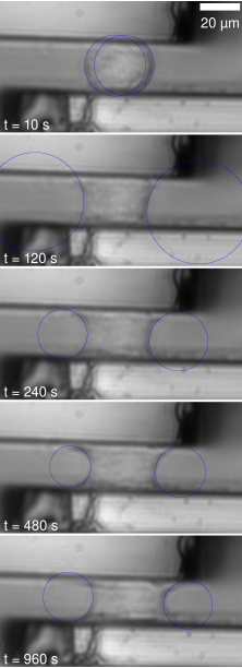
(a)

(b)

Supplementary Fig. S1:

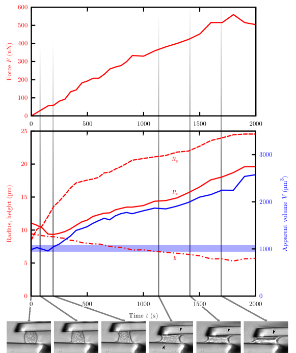
Supplementary Fig. S2:

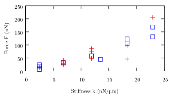
Supplementary Fig. S3:

Supplementary Fig. S4:

References

- [1] F. R. Turner and A. P. Mahowald. Scanning electron microscopy of drosophila melanogaster embryogenesis: II. Gastrulation and segmentation. Develop. Biol., 57:403–416, 1977.
- [2] A. Engler, Lucie Bacakova, C. Newman, A. Hategan, M. Griffin, and D. E. Discher. Substrate compliance versus ligand density in cell on gel responses. Biophys. J., 86:617–628, 2004.
- [3] T. Yeung, P. C. Georges, L. A. Flanagan, B. Marg, M. Ortiz, M. Funaki, N. Zahir, W. Ming, V. Weaver, and P. A. Janmey. Effects of substrate stiffness on cell morphology, cytoskeletal structure, and adhesion. Cell Motil. Cytoskeleton, 60:24–34, 2005.
- [4] A. Saez, M. Ghibaudo, A. Buguin, P. Silberzan, and B. Ladoux. Rigidity-driven growth and migration of epithelial cells on microstructured anisotropic substrates. Proc. Natl. Acad. Sci. USA, 104:8281–8286, 2007.
- [5] J. Zhong, J. B. Baquiran, N. Bonakdar, J. Lees, Y. Wooi Ching, E. Pugacheva, B. Fabry, and G. M. O’Neill. NEDD9 stabilizes focal adhesions, increases binding to the extra-cellular matrix and differentially effects 2D versus 3D cell migration. PLoS one, 7:e35058, 2012.
- [6] P. E. Young, A. M. Richman, A. S. Ketchum, and D. P. Kiehart. Morphogenesis in Drosophila requires nonmuscle myosin heavy chain function. Genes Dev., 7:29–41, 1993.
- [7] R. J. Pelham Jr. and Y. Wang. Cell locomotion and focal adhesions are regulated by substrate flexibility. Proc Natl Acad Sci USA, 94:13661–13665, 1997.
- [8] M. E. Chicurel, C. S. Chen, and D. E. Ingber. Cellular control lies in the balance of forces. Curr. Opin. Cell Biol., 10:232–239, 1998.
- [9] A. L. Zajac and D. E. Discher. Cell differentiation through tissue elasticity-coupled, myosin-driven remodeling. Curr. Opin. Cell Biol., 20:609–615, 2008.
- [10] Y. Cai, O. Rossier, N. C. Gauthier, N. Biais, M.-Antoine Fardin, X. Zhang, L. W. Miller, B. Ladoux, V. W. Cornish, and M. P. Sheetz. Cytoskeletal coherence requires myosin-IIA contractility. J. Cell Sci., 123:401–423, 2010.
- [11] D. E. Discher, P. Janmey, and Y. Wang. Tissue cells feel and respond to the stiffness of their substrate. Science, 310:1139–1143, 2005.
- [12] V. Vogel and M. Sheetz. Local force and geometry sensing regulate cell functions. Nat. Rev. Mol. Cell Biol., 7:265–275, 2006.
- [13] D. Mitrossilis, J. Fouchard, A. Guiroy, N. Desprat, N. Rodriguez, B. Fabry, and A. Asnacios. Single-cell response to stiffness exhibits muscle-like behavior. Proc. Natl. Acad. Sci. USA, 106:18243–18248, 2009.
- [14] K. D. Webster, A. Crow, and D. A. Fletcher. An afm-based stiffness clamp for dynamic control of rigidity. PLoS ONE, 6:e17807, 2011.
- [15] A. Crow, K. D. Webster, E. Hohlfeld, W. P. Ng, P. Geissler, and D. A. Fletcher. Contractile equilibration of single cells to step changes in extracellular stiffness. Biophys. J., 102:443–451, 2012.
- [16] L. Trichet, J. Le Digabel, R. J. Hawkins, S. R. K. Vedula, M. Gupta, C. Ribrault, P. Hersen, R. Voituriez, and B. Ladoux. Evidence of a large-scale mechanosensing mechanism for cellular adaptation to substrate stiffness. Proc. Natl. Acad. Sci. USA, 109:6933–6938, 2012.
- [17] O. M. Rossier, N. Gauthier, N. Biais, W. Vonnegut, M.-A. Fardin, P. Avigan, E. R. Heller, A. Mathur, S. Ghassemi, M. S. Koeckert, J. C. Hone, and M. P. Sheetz. Force generated by actomyosin contraction builds bridges between adhesive contacts. EMBO J., 29:1033–1044, 2010.
- [18] A. Zemel, F. Rehfeldt, A. E. X. Brown, D. E. Discher, and S. A. Safran. Optimal matrix rigidity for stress-fibre polarization in stem cells. Nature Phys., 6:468–473, 2010.
- [19] P. Marcq, N. Yoshinaga, and J. Prost. Rigidity sensing explained by active matter theory. Biophys. J., 101:L33–L35, 2011.
- [20] M. Yamamoto. The visco-elastic properties of network structure: I. General formalism. J. Phys. Soc. Jpn, 11:413–421, 1956.
- [21] A. F. Huxley. Muscle structure and theories of contraction. Prog. Biophys. Biophys. Chem., 7:255–318, 1957.
- [22] M. Kovács, K. Thirumurugan, P. J. Knight, and J. R. Sellers. Load-dependent mechanism of nonmuscle myosin 2. Proc. Natl. Acad. Sci. USA, 104:9994–9999, 2007.
- [23] S. Mukhina, Y. Wang, and M. Murata-Hori. -actinin is required for tightly regulated remodeling of the actin cortical network during cytokinesis. Dev. Cell, 13:554–565, 2007.
- [24] M. Fritzsche, A. Lewalle, T. Duke, K. Kruse, and G. Charras. Analysis of turnover dynamics of the submembranous actin cortex. Mol. Biol. Cell, 24:757–767, 2013.
- [25] A. Vaziri and A. Gopinath. Cell and biomolecular mechanics in silico. Nature Mater., 7:15–23, 2008.
- [26] A. K. Harris, P. Wild, and D. Stopak. Silicone rubber substrata: a new wrinkle in the study of cell locomotion. Science, 208:177–179, 1980.
- [27] X. He and M. Dembo. On the mechanics of the first cleavage division of the sea urchin egg. Exp. Cell Res., 233:252–273, 1997.
- [28] K. Kruse, J.F. Joanny, F. Jülicher, J. Prost, and K. Sekimoto. Generic theory of active polar gels: a paradigm for cytoskeletal dynamics. Eur. Phys. J. E, 16:5–16, 2005.
- [29] M. Soares e Silva, M. Depken, B. Stuhrmann, M. Korsten, F. C. MacKintosh, and G. H. Koenderink. Active multistage coarsening of actin networks driven by myosin motors. Proc. Natl. Acad. Sci. USA, 108:9408–9413, 2012.
- [30] D. Mitrossilis, J. Fouchard, D. Pereira, F. Postic, A. Richert, M. Saint-Jean, and A. Asnacios. Real-time single cell response to stiffness. Proc. Natl. Acad. Sci. USA, 107:16518–16523, 2010.
- [31] A. Saez, A. Buguin, P. Silberzan, and B. Ladoux. Is the mechanical activity of epithelial cells controlled by deformations or forces? Biophys. J., 89:L52–L54, 2005.
- [32] T. J. Mitchison and L. P. Cramer. Actin-based cell motility and cell locomotion. Cell, 84:371–379, 1996.
- [33] M. F. Fournier, R. Sauser, D. Ambrosi, J.-J. Meister, and A. B. Verkhovsky. Force transmission in migrating cells. J. Cell Biol., 188:287–297, 2010.
- [34] T. D. Pollard, L. Blanchoin, and R. D. Mullins. Molecular mechanisms controlling actin filament dynamics in nonmuscle cells. Annu. Rev. Biophys. Biomol. Struct., 29:545–576, 2000.
- [35] A. Ponti, M. Machacek, S. L. Gupton, C. M. Waterman-Storer, and G. Danuser. Two distinct actin networks drive the protrusion of migrating cells. Science, 305:1782–1786, 2004.
- [36] J. V. Small and G. P. Resch. The comings and goings of actin: coupling protrusion and retraction in cell motility. Curr. Opinion Cell Biol., 17:517–523, 2005.
- [37] E. Fällman, S. Schedin, J. Jass, B.-E. Uhlin, and O. Axner. The unfolding of the P pili quaternary structure by stretching is reversible, not plastic. EMBO rep., 6:52–56, 2005.
- [38] W. Federle, E. L. Brainerd, T. A. McMahon, and B. Hölldobler. Biomechanics of the movable pretarsal adhesive organ in ants and bees. Proc. Natl. Acad. Sci. USA, 98:6215, 2001.
- [39] A. V. Hill. The heat of shortening and the dynamic constants of muscle. Proc. R. Soc. Lond. B, 126:136–195, 1938.
- [40] G. B. West, W. H. Woodruff, and J H. Brown. Allometric scaling of metabolic rate from molecules and mitochondria to cells and mammals. Proc. Natl. Acad. Sci. USA, 99:2473–2478, 2002.
- [41] N. Desprats, A. Guiroy, and A. Asnacios. Microplates-based rheometer for a single living cell. Rev. Sci. Instrum., 77:055111, 2006.

References

- [1] Stamenović D, Mijailovich SM, Tolić-Nørrelykke IM, Wang N (2002) Cell prestress. II. Contribution of microtubules. Am J Physiol Cell Physiol 282:C617–C624.
- [2] Wottawah F, et al. (2005) Optical rheology of biological cells. Phys Rev Lett 94:098103.
- [3] Green MS, Tobolsky AV (1946) A new approach to the theory of relaxing polymeric media. J Chem Phys 14:80–92.
- [4] Vaccaro A, Marrucci G (2000) A model for the nonlinear rheology of associating polymers. J Non-Newtonian Fluid Mech 92:261–273.
- [5] Larson RG (1999) The structure and rheology of complex fluids. Topics Chem. Engng (Oxford Univ. Press).
- [6] Broedersz CP, et al. (2010) Cross-link governed dynamics of biopolymer networks. Phys Rev Lett 105:238101.
- [7] Debold EP, Patlak JB, Warshaw DM (2005) Slip sliding away: Load-dependence of velocity generated by skeletal muscle myosin molecules in the laser trap. Biophys J 89:L34–L36.
- [8] Rubinstein B, et al. (2009) Actin-myosin viscoelastic flow in the keratocyte lamellipod. Biophys J 97:1853–1863.
- [9] Williams WO (2011) Huxley’s model of muscle contraction with compliance. J Elas 105:365–380.
- [10] Zemel A, Rehfeldt F, Brown AEX, Discher DE, Safran SA (2010) Cell shape, spreading symmetry, and the polarization of stress-fibers in cells. J Phys: Condens Matter 22:194110.
- [11] Curtis A, Aitchison G, Tsapikouni T (2006) Orthogonal (transverse) arrangements of actin in endothelia and fibroblasts. J R Soc Interface 3:753–756.
- [12] Bischofs I, Klein F, Lehnert D, Bastmeyer M, Schwarz U (2008) Filamentous network mechanics and active contractility determine cell and tissue shape. Biophys J 95:3488–3496.
- [13] Jiang H, Sun SX (2013) Cellular pressure and volume regulation and implications for cell mechanics. Biophys J 105:609–619.