LOOL: Mathematica package for evaluating
leading order one loop functions

Abstract

One-loop functions with loop masses larger than external masses and momenta can always be expanded in terms of external masses and momenta. The precision requested for observables determines the number of the expansion terms retained in the evaluation. The evaluation of these expansion terms turns out to be much simpler than the exact evaluation of the corresponding one-loop function. Here we present the program which evaluates those expansion terms.

This Mathematica package provides two subroutines. First one performs analytical evaluation of basic one loop integrals. The second one is used to construct composite functions out of those integrals. Composite functions thus obtained are ready for numerical evaluation with literary no time consumption.

1 Introduction

Evaluation of loop integrals is always a challenging technicality, both analytically and numerically. Consequently, there have been numerous attempts to make computer algorithms which will make these computations both fast and automatic. Among various attempts, one can stress out Mathematica packages such as LoopTools [1], and ANT [2].

Although these and similar packages can be extremely useful in numerous calculations, they didn’t quite match our needs when dealing with charge lepton flavor violation (CLFV) processes [3, 4]. For that purpose, we have developed a package specialized in analytical and numerical evaluation of the loop functions expanded with respect to the momenta and masses of the external charged leptons, while keeping only the leading non-zero terms. Some of these methods were discussed in the Appendix B in Ref. [5], while the very concept of mass and momenta expansion was discussed in Refs. [6, 7, 8, 9, 10].

This package is written for Wolfram Mathematica, with the idea of being easy and straightforward to install and apply for various cases.

2 Installation and startup

The package can be downloaded from http://lool.hepforge.org. Once downloaded, it can be loaded into the Mathematica notebook in a usual manner,

<< "/path/to/file/LOOL.m"

3 Basic integrals

Any given one-loop amplitude can be expanded over the external masses and momenta [11]. The expansion terms can in turn be expressed via dimensionless loop integrals.

$$\bar{J}^{m}_{n_{1}n_{2}\dots n_{k}}(\lambda_{1},\lambda_{2},\dots,\lambda_{k}) =\frac{(\mu^{2})^{2-D/2}}{(M^{2}_{W})^{D/2+m-\sum_{i}n_{i}}}\int\frac{d^{D}\ell}{(2\pi)^{D}}\frac{(\ell^{2})^{m}}{\prod_{i=1}^{k}(\ell^{2}-m_{i}^{2})^{n_{i}}}$$

$$=\frac{i(-1)^{m-\sum_{i}n_{i}}}{(4\pi)^{D/2}\Gamma(\frac{D}{2})}\Big{(}\frac{\mu^{2}}{M_{W}^{2}}\Big{)}^{2-D/2}\int_{0}^{\infty}\frac{dxx^{D/2-1+m}}{\prod_{i=1}^{k}(x+\lambda_{i})^{n_{i}}}\,,$$ (1)

where $m_{i}$ are loop particle masses, $n_{i}$ are the exponents of the propagator denominators, $\lambda_{i}=m_{i}^{2}/M_{W}^{2}$ are dimensionless mass parameters and $\mu$ is ’t Hooft’s renormalization mass scale. For convergent integrals, one may set $D=4$, whilst for divergent integrals one takes $D=4-2\epsilon$. Factor $i/(4\pi)^{2}$ is pulled out from all integrals. Thus, for finite integrals one obtains:

$$\bar{J}^{m}_{n_{1}n_{2}\dots n_{k}}(\lambda_{1},\lambda_{2},\dots,\lambda_{k})\ \equiv\ \frac{i}{(4\pi)^{2}}\ J^{m}_{n_{1}n_{2}\dots n_{k}}(\lambda_{1},\lambda_{2},\dots,\lambda_{k})\;.$$ (2)

On the other hand, the divergent integrals are written down as a sum of a divergent and constant term and a finite mass-dependent term:

$$\bar{J}^{m}_{n_{1}n_{2}\dots n_{k}}(\lambda_{1},\lambda_{2},\dots\lambda_{k})\ \equiv\ \frac{i}{(4\pi)^{2}}\ \big{[}\frac{1}{\varepsilon}+\mbox{const}+J^{m}_{n_{1}n_{2}\dots n_{k}}(\lambda_{1},\lambda_{2},\dots,\lambda_{k})\big{]}\,.$$ (3)

Due to GIM-like mechanisms (see for example Eqs. (2.9) and (2.10) in Ref. [12]), the “divergent+constant” terms usually don’t have a role in evaluating the amplitudes. In that case, all amplitudes can be expressed in terms of finite mass dependent functions $J^{m}_{n_{1}n_{2}\dots}(\lambda_{1},\lambda_{2},\dots)$, which we call the basic loop integrals.

These integrals can be evaluated using JInt subroutine, which has the following syntax:

JInt[{m, n1, n2, ...}, {x, y, ...}]

Notice that this function is called with two variable lists. First one stands for $m,n_{1},n_{2},\ldots,n_{k}$, while the second one stands for $\lambda_{1},\lambda_{2},\ldots,\lambda_{k}$, as noted in Eq. (3). The parameter $k$ can assume values $k=1,2,3,4$, corresponding to the tadpole, self energy, triangle and box loop integrals, respectively. This can be easy extended to any $k$-point function.

This function returns two expressions. First value correspond to the expression for the basic loop integral $J^{m}_{n_{1}n_{2}\dots}(\lambda_{1},\lambda_{2},\dots)$, while the second one gives the accompanied “divergent+constant” terms.

Example 1

Evaluate the integral $J^{1}_{111}(x,y,z)$.

Solution

According to the subroutine syntax, one easily obtains:

In[1]  := JInt[{1, 1, 1, 1}, {x, y, z}]
Out[1] := {(x^2*(-y+z)*Log[x] + y^2*(x-z)*Log[y] +
          (-x+y)*z^2*Log[z])/((x-y)*(x-z)*(y-z)),
          1 - EulerGamma + \[Epsilon]^(-1) + Log[4*Pi] + 2*Log[\[Mu]]}

Or written in the more readable fashion,

$$J^{1}_{111}(x,y,z)=\frac{x^{2}(z-y)\ln(x)+y^{2}(x-z)\ln(y)+z^{2}(y-x)\ln(z)}{(x-y)(x-z)(y-z)}+\frac{1}{\varepsilon}+2\ln(\mu)-\gamma+1+\ln(4\pi)\,,$$

where $\gamma=0.5772\ldots$ is the Euler-Mascheroni constant.

4 Composite functions

For concrete applications, one wants to numerically evaluate functions which are composed out of the $J$-integrals listed above. This can be done using the second subroutine, CompositeF. This subroutine has the following syntax:

CompositeF[fun, {x, y, ...}]

This function is called with two arguments. First argument stands for some function composed out of $J$-integrals, and second one lists the arguments of this very function.

CompositeF subroutine results with function which is numerically ready for evaluation, with all possible limits evaluated at once. The problem with numerical instability near the critical values which often occurs in Mathematica is elegantly solved by transforming decimal numbers into rational numbers just before the evaluation. For this reason, the final numerical result will always be given as a rational number, which, if necessary, can be expressed as a real number using Mathematica function N. The result of this approach can be seen in Fig. 1.

      

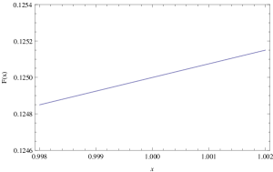
Figure 1: Behavior of function $F(x)=J^{1}_{31}(1,x)+J^{2}_{41}(1,x)+x\left(\frac{1}{2}J^{1}_{41}(1,x)-J^{0}_{31}(1,x)\right)+\frac{5}{6}$. On the left panel one can notice the numerical instability for critical values when real numbers are used, while the right panel displays the evaluation of the same function using rational numbers (obtained by the CompositeF function).

The following example should further illustrate the use of CompositeF.

Example 2

Construct the following composite function

$$F(x,y,z)=J^{1}_{1111}(1,z,x,y)+xyJ^{0}_{1111}(1,z,x,y)+\frac{xy}{\tan^{2}\beta}J^{0}_{211}(z,x,y)\,,$$

and numerically evaluate $F(0,1,1)$, supposing the existence of GIM-mechanism.

Solution

First step is to evaluate the basic loop integrals. Due to the assumed existence of GIM-mechanism, we are not interested in the constant terms. After the definition of the relevant $J$-integrals, one can easily define the composite function and simply evaluate it for the given values.

In[1]  := J11111[x_, y_, z_, w_] = JInt[{1, 1, 1, 1, 1}, {x, y, z, w}][[1]]
Out[1] := -((w^2*Log[w])/((w-x)*(w-y)*(w-z))) + (x^2*Log[x])/((w-x)*(x-y)*(x-z)) +
          (y^2*Log[y])/((w-y)*(-x+y)*(y-z)) + (z^2*Log[z])/((w-z)*(-x+z)*(-y+z))

In[2]  := J01111[x_, y_, z_, w_] = JInt[{0, 1, 1, 1, 1}, {x, y, z, w}][[1]]
Out[2] := -((w*Log[w])/((w-x)*(w-y)*(w-z))) + (x*Log[x])/((w-x)*(x-y)*(x-z)) +
          (y*Log[y])/((w-y)*(-x+y)*(y-z)) + (z*Log[z])/((w-z)*(-x+z)*(-y+z))

In[3]  := J0211[x_, y_, z_] = JInt[{0, 2, 1, 1}, {x, y, z}][[1]]
Out[3] := ((y-z)*(x^2-y*z)*Log[x] + (x-z)*(-((x-y)*(y-z)) + y*(-x+z)*Log[y]) +
          (x-y)^2*z*Log[z])/((x-y)^2*(x-z)^2*(y-z))

In[4]  := F[x_, y_, z_] = CompositeF[J11111[1, z, x, y] + x*y*J01111[1, z, x, y] +
          (x*y)/tb^2*J0211[z, x, y], {x, y, z}];

In[5]  := F[0, 1, 1]
Out[5] := -1/2

While the first four steps do take certain amount of time to evaluate, last step literary takes zero time to complete. That is the reason why it is of great importance to use the equal sign “=” rather than the definition sign “:=” when defining the functions.

In order to make future evaluations time effective, one is advised to save the once evaluated composite function into a separate file,

Save["some_file.dat", {F}]

which can be invoked in any other Mathematica notebook, for example

In[1]  := <<"\path\to\file\some_file.dat";

In[2]  := F[0, 1, 1]
Out[2] := -1/2

5 Conclusion

We have developed and presented a Mathematica package LOOL which calculates leading order one loop functions, both analytically and numerically. The composite functions composed out of basic loop integrals are evaluated only once, including all possible limits. Additionally, the problem with numerical instability near the critical values is successfully solved by dealing with rational rather to real numbers.

References

References

- [1] T. Hahn, M. Perez-Victoria, Automatized one loop calculations in four-dimensions and D-dimensions, Comput.Phys.Commun. 118 (1999) 153–165. arXiv:hep-ph/9807565, doi:10.1016/S0010-4655(98)00173-8.
- [2] P. W. Angel, Y. Cai, N. L. Rodd, M. A. Schmidt, R. R. Volkas, Testable two-loop radiative neutrino mass model based on an effective operator, JHEP 1310 (2013) 118. arXiv:1308.0463, doi:10.1007/JHEP10(2013)118.
- [3] A. Ilakovac, A. Pilaftsis, L. Popov, Charged Lepton Flavour Violation in Supersymmetric Low-Scale Seesaw Models, Phys. Rev. D 87 (2013) 053014. arXiv:1212.5939, doi:10.1103/PhysRevD.87.053014.
- [4] A. Ilakovac, A. Pilaftsis, L. Popov, Lepton Dipole Moments in Supersymmetric Low-Scale Seesaw Models, Phys.Rev. D89 (2014) 015001. arXiv:1308.3633, doi:10.1103/PhysRevD.89.015001.
- [5] L. Popov, Lepton flavor violation in supersymmetric low-scale seesaw models, Ph.D. thesis, University of Zagreb (2013). arXiv:1312.1068.
- [6] M. Veltman, Second Threshold in Weak Interactions, Acta Phys.Polon. B8 (1977) 475.
- [7] J. Fleischer, O. Tarasov, Calculation of Feynman diagrams from their small momentum expansion, Z.Phys. C64 (1994) 413–426. arXiv:hep-ph/9403230, doi:10.1007/BF01560102.
- [8] O. Tarasov, An Algorithm for small momentum expansion of Feynman diagramsarXiv:hep-ph/9505277.
- [9] O. Tarasov, A New approach to the momentum expansion of multiloop Feynman diagrams, Nucl.Phys. B480 (1996) 397–412. arXiv:hep-ph/9606238, doi:10.1016/S0550-3213(96)00466-X.
- [10] V. A. Smirnov, Applied asymptotic expansions in momenta and masses, Springer Tracts Mod.Phys. 177 (2002) 1–262.
-
[11]
J. Van Tran (Ed.),
Phenomenology of Gauge
Theories: Proceedings of the Leptonic Session of the Nineteenth Rencontre de
Moriond, Moriond proceedings, Editions Frontieres, La Plagne-Savoie, France,
1984, p 78.
URL http://books.google.hr/books?id=n1hrCGUIJY8C - [12] A. Ilakovac, A. Pilaftsis, Flavor violating charged lepton decays in seesaw-type models, Nucl. Phys. B 437 (1995) 491. arXiv:hep-ph/9403398, doi:10.1016/0550-3213(94)00567-X.