$\Delta(1232)$ Resonance Contribution to Two-Photon Exchange in Electron-Proton Scattering Revisited

Abstract

We revisit the question of the contributions of two-photon exchange with $\Delta(1232)$ excitation to the electron-proton scattering in a hadronic model. Three improvements over the previous calculations are made, namely, correct vertex function for $\gamma N\rightarrow\Delta$, realistic $\gamma N\Delta$ form factors, and coupling constants. The discrepancy between the values of $R\equiv\mu_{p}G_{E}/G_{M}$ extracted from Rosenbluth technique and polarization transfer method can be reasonably accounted for if the data of Andivahis et al. (Phys. Rev. D 50, 5491 (1994)) are analyzed. However, substantial discrepancy remains if the data of Qattan et al. (nucl-ex/0610006) are used. For the ratio $R^{\pm}$ between $e^{\pm}p$ scatterings, our predictions appear to be in satisfactory agreement with the preliminary data from VEPP-3. The agreement between our model predictions and the recent measurements on single spin asymmetry, transverse and longitudinal recoil proton polarizations ranges from good to poor.

1 Introduction

Proton is the only stable hadron and hence most amenable to experimental measurement in the hadron structure study. Determination of the proton form factors via electron elastic scattering started in the 1950’s. Nearly half of a century of efforts yield the so-called scaling law, i.e., $R=\mu_{p}G_{E}/G_{M}\sim 1$ for $Q^{2}<6$ GeV², where $\mu_{p}$, $G_{E}$, and $G_{M}$ are the magnetic moment, Sach’s electric and magnetic form factors of the proton, respectively, as often quoted in textbooks. The measurements leading to the scaling law were all obtained from analyses of the data based on the one-photon exchange (OPE) approximation.

In the OPE approximation, the proton’s electric and magnetic form factors (FFs) can be extracted from the reduced differential cross section $\sigma_{R}$ of the electron-proton $\it(ep)$ elastic scattering as one has

$$\sigma_{R}(Q^{2},\epsilon)\equiv\frac{d\sigma}{d\Omega_{lab}}\frac{\epsilon(1+\tau)}{\tau\sigma_{Mott}}=G_{M}^{2}+\frac{\epsilon}{\tau}G_{E}^{2},$$ (1)

where $\tau=Q^{2}/4M_{N}^{2},\,\,\epsilon^{-1}=1+2(1+\tau)tan^{2}\theta/2,\,\,Q^{2}=-q^{2}$ the momentum transfer squared, $M_{N}$ the nucleon mass, $\theta$ the laboratory scattering angle, $0\leq\epsilon\leq 1$, and $\sigma_{Mott}$ is the Mott cross section for the scattering from a point particle,

$$\sigma_{Mott}\equiv\frac{\alpha^{2}E_{3}cos^{2}\frac{\theta}{2}}{4E_{1}^{3}sin^{4}\frac{\theta}{2}},$$ (2)

with $E_{1}$ and $E_{3}$ the initial and final electron energies and $\alpha=e^{2}/4\pi$ the electromagnetic fine structure constant. For fixed $Q^{2}$, varying angle $\theta$, i.e. $\epsilon$, and adjusting incoming electron energy as needed to plot $\sigma_{R}$ versus $\epsilon$ will give the FFs, a method often called the Rosenbluth, or longitudinal-transverse (LT), separation technique.

The good times with scaling law ended when, at the turn of this century, a polarization transfer (PT) experiment carried out at JLab yielded values of $R$ markedly different from 1 in the range of $0.2<Q^{2}<8.5$ GeV ² [1, 2, 3, 4, 5]. The polarization experiment is based on a result shown in [6, 7] that, again in the OPE approximation, the ratio $R$ can be accessed in $ep$ scattering with longitudinally polarized electron by measuring the polarizations of the recoiled proton parallel $P_{l}$ and perpendicular $P_{t}$ to the proton momentum in the scattering plane,

$$R=\frac{\mu_{p}G_{E}}{G_{M}}=-\mu_{p}\sqrt{\frac{\tau(1+\epsilon)}{2\epsilon}}\frac{P_{t}}{P_{l}}.$$ (3)

Polarization transfer experiment of this kind is only possible recently at JLab. It came as a big surprise that the PT experiments yield values of $R$ deviate substantially from 1. It prompts intensive efforts, both experimentally and theoretically. The readers are referred to recent reviews [8, 9, 10] for details on these developments. In addition, a comprehensive exposition of the application of the soft-collinear effective theory (SCET) to the study of the two-photon exchange (TPE) corrections to the electron-proton scattering in the region where the kinematical variables describing the elastic ep scattering are moderately large momentum scales relative to the soft hadronic scale is presented in [11].

On the experimental side, a new global analysis of the world’s cross section data was carried out in [12]. It is found that the great majority of the measured cross sections were consistent with each other and the disagreement with polarization transfer measurements remains. A set of extremely high precision measurements of $R$ was later performed using a modified Rosenbluth technique [13, 14], with the detection of recoil proton to minimize the systematic uncertainties, and the discrepancy is again confirmed.

The immediate step taken, on the theoretical side, was to carefully reexamine the radiative corrections which were known to be as large as $30\%$ of the uncorrected cross section in certain kinematics. Of various radiative corrections, only proton-vertex and two-photon exchange (TPE) corrections contained $\epsilon$ dependence. The proton-vertex corrections had been investigated thoroughly in [15] and found to be negligible. Realistic evaluations of the TPE corrections are hence called for to see whether they can explain the discrepancy.

A semi-quantittative analysis [16] quickly established that the discrepancy can possibly be explained by a two-photon exchange correction which would not destroy the linearity of the Rosenbluth plot. The ensuing theoretical investigation of the two-photon exchange effects include hadronic [17, 18, 19] and partonic model [20, 21] calculations, phenomenological parametrizations [22, 23], dispersion approach [25, 24, 26, 27, 28], and pQCD calculations [29, 30]. They all have found that TPE effects can account for more than half of the discrepancy.

The hadronic model calculations of the effects of TPE with nucleon intermediate states, denoted as TPE-N hereafter, have established that it is important to employ realistic $\gamma NN$ form factors [17, 19]. For the inelastic contributions, it has been demonstrated in [31] that $\Delta(1232)$ dominates in the case of target-normal spin asymmetry. The effects of TPE with $\Delta$ excitation, denoted as TPE-$\Delta$ hereafter, in the cross sections and the form factors have been studied in [18, 27, 28]. However, there are rooms for improvement in three aspects of these calculations to arrive at a reliable estimate of the TPE-$\Delta$ effects. First, as was pointed out in [32], the expression for the vertex function of $\gamma N\rightarrow\Delta$ used in [18] has the incorrect sign for the Coulomb quadrupole coupling, though it was not considered in [27]. Next is that the $\gamma N\Delta$ form factors employed in [18] are not realistic which, as we learn in the case of TPE-N, needs to be studied. Lastly, both [18, 27] set the Coulomb quadrupole coupling to be zero, which is again not satisfactory since recent pion electroproduction experiments and the LQCD results indicate that the ratio of Coulomb quadrupole (C2) over magnetic dipole (M1), denote by $R_{SM}=C2/M1$ grows more negative with increasing $Q^{2}$ [33, 34, 35, 37, 36]. The theoretical understandings of the discrepancy between LT and PT experiments, as well as the TPE contributions are still ongoing. It is important to have the results from various model calculations as accurate as possible so as to understand the strength and the weakness of different approaches and shed light for the further study. Accordingly, we set out in this study to improve the previous calculations of the effects of TPE-$\Delta$ excitation [18] on the three aspects described in the above.

This article is organized as follows. In Sec. II, we give the explicit expression for the amplitude of two-photon exchange with $\Delta$ in the intermediate states and elaborate on the details of the three improvements we will implement. They are, (1) the correct expression for the $\gamma N\rightarrow\Delta$ with Coulomb quardrupole coupling; (2) the realistic $\gamma N\rightarrow\Delta$ form factors; and (3) Coulomb quadrupole $\gamma N\rightarrow\Delta$ coupling constant as given by the recent experiment. Results with the implementation of each of these three improvements are presented in Sec. III and compared with those obtained in [18] to demonstrate their importance. We then proceed to present results, obtained with all three improvements combined, for reduced cross sections, extracted $R$ in LT method, ratio $R^{\pm}$ between positron-proton and electron-proton cross sections, single spin asymmetries, longitudinal and transverse polarizations of the recoil proton $P_{l},P_{t}$ and their ratio $R_{PT}=-\mu_{p}\sqrt{\tau(1+\epsilon)/2\epsilon}P_{t}/P_{l}$. In Sec. IV, we summarize our results.

2 Two-photon exchange with $\Delta(1232)$ excitation in elastic electron-proton scattering

In this section, we discuss the evaluation of the two-photon exchange (TPE) diagrams with $\Delta(1232)$ excitation TPE-$\Delta$, as depicted in Fig.  1,

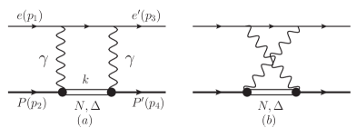
Figure 1: Two-photon exchange diagrams with $\Delta$ excitation for elastic ep scattering.

in a simple hadronic model. The amplitude for the box diagram in Fig. 1(a) is given as,

$$M^{(a,\Delta)} = -i\int\frac{d^{4}k}{(2\pi)^{4}}\overline{u}(p_{3})(-ie\gamma_{\mu})\frac{i(p\!\!\!\!/_{1}+p\!\!\!\!/_{2}-k\!\!\!\!/)}{(p_{1}+p_{2}-k)^{2}-m_{e}^{2}+i\varepsilon}$$ (4)

$$\times(-ie\gamma_{\nu})u(p_{1})\frac{-i}{(p_{4}-k)^{2}+i\varepsilon}\times\frac{-i}{(k-p_{2})^{2}+i\varepsilon}$$

$$\times\overline{u}(p_{4})\Gamma^{\mu\alpha}_{\gamma\Delta\rightarrow N}(k,p_{4}-k)\frac{-i(k\!\!\!\!/+M_{\Delta})P_{\alpha\beta}^{3/2}(k)}{k^{2}-M_{\Delta}^{2}+i\varepsilon}$$

$$\times\Gamma^{\nu\beta}_{\gamma N\rightarrow\Delta}(k,k-p_{2})u(p_{2}),$$

where

$$P_{\alpha\beta}^{3/2}(k)=g_{\alpha\beta}-\frac{\gamma_{\alpha}\gamma_{\beta}}{3}-\frac{(k\!\!\!\!/\gamma_{\alpha}k_{\beta}+k_{\alpha}\gamma_{\beta}k\!\!\!\!/)}{3k^{2}},$$ (5)

is the spin-3/2 projector. Amplitude for the cross-box diagram Fig. 1(b) can be written down in similar manner. The amplitude in Eq. (4) is IR finite because when the four-momentum of the photon approaches zero, the $\gamma N\Delta$ vertex functions $\Gamma^{\prime}s$ also approaches zero. Therefore we do not have to include an infinitesimal photon mass in the photon propagators to regulate the IR divergence in Eq. (4). The vertex functions $\Gamma^{\prime}s$ for $\gamma\Delta\rightarrow N$ and $\gamma N\rightarrow\Delta$ are defined by

$$\overline{u}(p+q)\Gamma^{\mu\alpha}_{\gamma\Delta\rightarrow N}(p,q)u^{\Delta}_{\alpha}(p) = -ie\langle N(p+q)|J^{\mu}_{EM}|\Delta(p)\rangle,$$ (6)

$$\overline{u}^{\Delta}_{\beta}(p)\Gamma^{\nu\beta}_{\gamma N\rightarrow\Delta}(p,q)u(p-q) = -ie\langle\Delta(p)|J^{\nu}_{EM}|N(p-q)\rangle,$$ (7)

where the $q^{\prime}s$ in both $\Gamma^{\mu\alpha}_{\gamma\Delta\rightarrow N}(p,q)$ and $\Gamma^{\beta\nu}_{\gamma N\rightarrow\Delta}$ refer to the incoming momentum of the photon, as in [18].

We now elaborate, in the followings, on the three improvements over the previous calculations we will carry out in this study.

2.1 Relation between vertex functions of $\gamma\Delta\rightarrow N$ and $\gamma N\rightarrow\Delta$

The correct relations between the two vertex functions for $\gamma\Delta\rightarrow N$ and $\gamma N\rightarrow\Delta$ are

$$\Gamma_{\gamma\Delta\rightarrow N}(p,q)=-\gamma_{0}[\Gamma_{\gamma N\rightarrow\Delta}(p,-q)]^{\dagger}\gamma_{0},$$ (8)

with $q^{\prime}s$ in both sides of the above Eq. (8) denote the incoming momentum of the photon. It follows from the fact that electromagnetic current is Hermitian. However, in [18, 38] the following relation between $\Gamma_{\gamma N\rightarrow\Delta}$ and $\Gamma_{\gamma\Delta\rightarrow N}$ has been used:

$$\Gamma_{\gamma\Delta\rightarrow N}(p,q)=\gamma_{0}[\Gamma_{\gamma N\rightarrow\Delta}(p,q)]^{\dagger}\gamma_{0}.$$ (9)

Specifically, with the inclusion of the form factors, vertex function $\Gamma_{\gamma\Delta\rightarrow N}^{\mu\alpha}$ takes the form

$$\Gamma_{\gamma\Delta\rightarrow N}^{\mu\alpha}(p,q) = -i\sqrt{\frac{2}{3}}{\displaystyle\frac{e}{2M_{\Delta}^{2}}}\bigg{\{}g_{1}F^{(1)}_{\Delta}(q^{2})[g^{\mu\alpha}p\!\!\!\!/q\!\!\!\!/-$$ (10)

$$p^{\mu}\gamma^{\alpha}q\!\!\!\!/-\gamma^{\mu}\gamma^{\alpha}p\cdot q+\gamma^{\mu}p\!\!\!\!/q^{\alpha}]$$

$$+g_{2}F^{(2)}_{\Delta}(q^{2})\left[\,p^{\mu}q^{\alpha}-g^{\mu\alpha}p\cdot q\,\right]$$

$$+(g_{3}/M_{\Delta})F^{(3)}_{\Delta}(q^{2})[q^{2}(p^{\mu}\gamma^{\alpha}-g^{\mu\alpha}p\!\!\!\!/)$$

$$+q^{\mu}(q^{\alpha}p\!\!\!\!/-\gamma^{\alpha}p\cdot q)]\bigg{\}}\gamma_{5}.$$

Eq. (8) then leads to

$$\Gamma_{\gamma N\rightarrow\Delta}^{\nu\beta}(p,q) = -i\sqrt{\frac{2}{3}}{\displaystyle\frac{e}{2M_{\Delta}^{2}}}\gamma_{5}\bigg{\{}g_{1}F^{(1)}_{\Delta}(q^{2})[g^{\nu\beta}q\!\!\!\!/p\!\!\!\!/$$ (11)

$$-p^{\nu}q\!\!\!\!/\gamma^{\beta}-\gamma^{\beta}\gamma^{\nu}p\cdot q+p\!\!\!\!/\gamma^{\nu}q^{\beta}]$$

$$+g_{2}F^{(2)}_{\Delta}(q^{2})[p^{\nu}q^{\beta}-g^{\nu\beta}p\cdot q]$$

$$-(g_{3}/M_{\Delta})F^{(3)}_{\Delta}(q^{2})[q^{2}(p^{\nu}\gamma^{\beta}-g^{\nu\beta}p\!\!\!\!/)$$

$$+q^{\nu}(q^{\beta}p\!\!\!\!/-\gamma^{\beta}p\cdot q)]\bigg{\}},$$

where at $Q^{2}=0$, $g_{i}^{\prime}s$ are related to the conventionally used magnetic dipole $G^{*}_{M}$, electric quadrupole $G^{*}_{E}$, and Coulomb quardrupole couplings $G^{*}_{C}$ form factors by [37],

$$g_{1} = \frac{3M_{\Delta}^{2}}{M_{N}(M_{\Delta}+M_{N})}(G^{*}_{M}-G^{*}_{E})$$

$$g_{2} = \frac{3M_{\Delta}^{2}(M_{\Delta}+3M_{N})}{M_{N}(M_{\Delta}^{2}-M_{N}^{2})}G^{*}_{E}+\frac{3M_{\Delta}^{2}}{M_{N}(M_{\Delta}+M_{N})}G^{*}_{M}$$

$$g_{3} = -\frac{3M_{\Delta}^{2}}{M_{N}(M_{\Delta}+M_{N})}\left(-\frac{M_{\Delta}+M_{N}}{(M_{\Delta}-M_{N})}G^{*}_{C}+\frac{4M_{\Delta}^{2}}{(M_{\Delta}-M_{N})^{2}}G^{*}_{E}\right),$$

However, if Eq. (9) is used, then one would get an expression for $\Gamma_{\gamma N\rightarrow\Delta}$ which would lead to the last term in Eq. (11) to carry a different sign, namely, the negative sign in front of $g_{3}$ in Eq. (11) becomes positive. Since in both [18, 38] $g_{3}$ was set to zero, this sign problem would not affect the results presented therein.

The difference between Eq. (8) and Eq. (9) incurs significant discrepancy in the results, in the case of corrections of $\gamma Z$ exchange with $\Delta$ excitation to the parity-violating electron-proton scattering, obtained in [39, 32] and [38] at the forward angles and higher $Q^{2}$. Similar situation can be expected to arise in the parity-conserving $ep$ scattering as well. In this study we use Eq. (8) because it is derived from the fact that the currents are Hermitian.

2.2 Realistic form factors for $\gamma N\Delta$ vertex

As demonstrated in [17, 19], the estimated contribution of TPE-N is reliable only if the employed nucleon form factors are realistic, similar situation can be expected to arise in the case with $\Delta$ intermediate states.

In [18], all three form factors $(F_{\Delta}^{(i)},\,\,i=1,3)$ in Eqs. (10, 11) are assumed to take the same form as

$$F^{(i)}_{\Delta}(q^{2})=F(q^{2})=\left(\frac{-\Lambda^{2}_{1}}{q^{2}-\Lambda^{2}_{1}}\right)^{2},\,(i=1,3),$$ (13)

with $\Lambda_{1}$ = 0.84 GeV.

In this investigation, the $\Delta$ form factors are taken to have the following forms,

$$F^{(1)}_{\Delta} = F^{(2)}_{\Delta}=\left(\frac{-\Lambda_{1}^{2}}{q^{2}-\Lambda_{1}^{2}}\right)^{2}\frac{-\Lambda_{3}^{2}}{q^{2}-\Lambda_{3}^{2}},\,$$

$$F^{(3)}_{\Delta} = \left(\frac{-\Lambda_{1}^{2}}{q^{2}-\Lambda_{1}^{2}}\right)^{2}\frac{-\Lambda_{3}^{2}}{q^{2}-\Lambda_{3}^{2}}\left[a\frac{-\Lambda_{2}^{2}}{q^{2}-\Lambda_{2}^{2}}+(1-a)\frac{-\Lambda_{4}^{2}}{q^{2}-\Lambda_{4}^{2}}\right],\,$$

with $\Lambda_{1}=0.84\,$GeV,$\,\Lambda_{2}=2\,\,$ GeV$,\,\Lambda_{3}=\sqrt{2}\,\,$GeV, $\Lambda_{4}$ = $0.2$ GeV, $a=-0.3.$ In Fig. 2, we compare the conventional magnetic dipole ($G^{*}_{M}$), the ratio of electric quadrupole (E2) over magnetic dipole (M1), and the ratio of Coulomb quadrupole (C2) over magnetic dipole (M1), denoted by $R_{EM}$ and $R_{SM}$ [37], respectively, resulting from the form factors given used in [18] and this study, as given in Eqs. (13, LABEL:D3), with the experimental data taken from [33, 34, 35]. The black solid curves, labeled as KBMT, denote the predictions as would be obtained with Eq. (13) as employed in [18]. They deviate strongly from the experimental data, especially for $G^{*}_{M}$ and $R_{EM}$. The red dashed curves, labeled as ZY, correspond to predictions as would be obtained with Eq. (LABEL:D3) and used in our study, agree well with the data except for $R_{EM}$ at $Q^{2}\sim 4-6\,$ GeV² where we purposely impose the prediction of PQCD to have $R_{EM}$ to approach one when $Q^{2}$ become infinity.

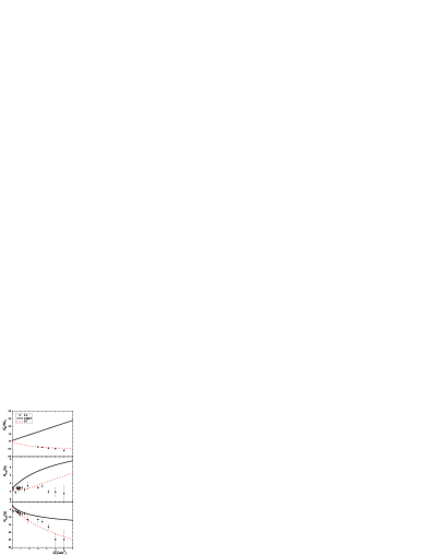
Figure 2: Comparison of the $\Delta$ form factor $G^{*}_{M}$, $R_{EM}$, and $R_{SM}$ used in [18] and this study with the experimental data [33, 34, 35].

2.3 $\gamma N\Delta$ coupling constants

The parameters used in this study are taken as $(g_{1},g_{2},g_{3})=(6.59,9.08,7.12)$ which are extracted from the most recent experiments [37]. In contrast, [18] use $(g_{1},g_{2},g_{3})=(7,9,0)$. The biggest difference lies with $g_{3}$ which corresponds to the Coulomb quardrupole coupling. Our value for $g_{3}$ is extracted from the most recent experiments and is quite large. For the finite $g_{3}$ case, since the corrected $N\rightarrow\Delta$ vertex function as given in Eq. (11) has a minus sign in front of $g_{3}$, while it would be positive if the prescription for this vertex function given in [18] is followed, significant difference in the predictions can be expected.

3 Results and discussions

The loop integrals with $\Delta$ intermediate state are infrared safe. We use computer package “FeynCalc” [40] and “LoopTools” [41] to carry out the calculations of integrals of Eq. (4).

In this section, we will first give the results of our calculation with each of the three improvements on the $\Delta$ contribution implemented separately, to demonstrate the importance of using correct $\gamma N\Delta$ vertex function, realistic form factors and coupling constants. Then we will proceed to present our results with all three improvements implemented together, as well as employing realistic $\gamma NN$ form factors used in [19], for the unpolarized cross sections, extracted ratio $R=\mu G_{E}/G_{M}$, ratio $R^{\pm}$ between $e^{+}p$ and $e^{-}p$ scatterings, single spin asymmetries $B_{n}$ and $A_{n}$, and polarization observables $P_{l},P_{t}$, and $R_{PT}$, and compare them with results and the model predictions of [42], as well as the data.

3.1 Separate effects of the three improvements: correct $\gamma N\Delta$ vertex function, realistic $\gamma N\Delta$ form factors, and coupling constants

As in [18], the corrections of the TPE to the unpolarized reduced cross section can be quantified as,

$$\sigma_{R} = [G_{M}^{2}+\frac{\epsilon}{\tau}G_{E}^{2}](1+\bar{\delta}_{N}+\delta_{\Delta})$$ (15)

$$= [G_{M}^{2}+\frac{\epsilon}{\tau}G_{E}^{2}](1+\Delta_{un}),$$

where $\bar{\delta}_{N}=\delta_{N}-\delta_{IR}(MT)$, with $\delta_{IR}(MT)$ the well-known Mo and Tsai’s radiative corrections [43, 44] which are removed from data in typical experimental analyses. $\Delta_{un}=\bar{\delta}_{N}+\delta_{\Delta}$ with $\delta_{N}$($\delta_{\Delta}$) denotes the correction obtained from the two-photon exchange diagrams with nucleons ($\Delta^{\prime}s$) in the intermediate states, respectively, as depicted in Fig. 1.

If we denote the Born scattering amplitude as $M_{B}$ and the two-photon exchange amplitudes with nucleon and $\Delta$ intermediate states as $M_{N}^{2\gamma}$ and $M_{\Delta}^{2\gamma}$, then to the first order in the electromagnetic coupling $\alpha=e^{2}/4\pi$, $\delta_{N,\Delta}$ are given as,

$$\delta_{N,\Delta}=2\frac{Re(M_{B}^{\dagger}M_{N,\Delta}^{2\gamma})}{\mid M_{B}\mid^{2}}.$$ (16)

$\delta_{N}$ was well studied in [17, 19]. For $\delta_{\Delta}$ in Eq. (16), we note that it is linear in $M_{\Delta}^{2\gamma}$. Since $\gamma N\Delta$ vertex appears twice in $M_{\Delta}^{2\gamma}$, $\delta_{\Delta}$ can then be expressed in a quadratic form in the $\gamma N\Delta$ coupling constants $g_{i}^{\prime}s$,

$$\delta_{\Delta}=\Sigma_{i,j=1}^{3}{C_{ij}g_{i}g_{j}}.$$ (17)

The values of $C_{ij}$’s vs. $\epsilon$ at $Q^{2}=3\,$GeV², are presented in Table 1, where only those with $i\leq j$ are given because $C_{ij}=C_{ji}$. It is seen that all $C_{i3}$’s are one to two orders smaller than the rest. We find that the values of $C_{i3}$’s are very sensitive $w.r.t.$ the form factors in that they would become comparable to the others if form factors of Eq. (13) are used.

In [18], they chose to write $\delta_{\Delta}=C_{MM}g^{2}_{M}+C_{ME}g_{M}g_{E}+C_{E}g^{2}_{E}+C_{C}g^{2}_{C}+C_{EC}g_{E}g_{C}+C_{MC}g_{M}g_{C}$ instead, where $g_{M}=g_{1},\,g_{E}=g_{2}-g_{1},\,g_{C}=g_{3}$. Our numbers would agree with those presented in Table I of [18] if their form factors of Eq. (13) are employed, wherein $C_{MC,EC}$ are found to be less than $10^{-10}$. In fact, both $C_{MC,EC}$ should be identically zero when the incorrect relation between $\Gamma_{\gamma N\rightarrow\Delta}$ and $\Gamma_{\gamma\Delta\rightarrow N}$ of Eq. (9) is used because one would then have $C_{i3}=-C_{3i},\,(i\neq 3)$.

$\varepsilon$	104 C11	104C12	104C22	106C13	106C23	106C33
0.1	-0.053	2.974	-1.015	-5.847	0.560	0.036
0.2	0.121	2.737	-1.048	-4.616	0.543	0.066
0.3	0.245	2.518	-1.054	-3.647	0.640	0.097
0.4	0.333	2.305	-1.036	-2.957	0.838	0.131
0.5	0.391	2.089	-0.991	-2.580	1.140	0.170
0.6	0.427	1.857	-0.918	-2.582	1.570	0.217
0.7	0.445	1.596	-0.809	-3.112	2.186	0.279
0.8	0.551	1.278	-0.647	-4.547	3.153	0.371
0.9	0.462	0.824	-0.376	-8.317	5.123	0.554

Table 1: $C_{ij}$ of Eq. (17) at $Q^{2}=3$ GeV² obtained with correct vertex $\gamma N\Delta$ function, realistic $\gamma N\Delta$ and $\gamma NN$ form factors, and coupling constants.

We first focus on the effects associated with the use of different vertex functions given in Eqs. (8, 9). In Fig. (3a), results for $\delta_{\Delta}$ vs. $\epsilon$ at $Q^{2}=3\,\,$GeV², with $g_{1}=7,g_{2}=9$, as considered in [18], are shown. The (red) dotted and the (black) solid curves, labeled as KBMT and using their $\gamma N\Delta$ vertex relation Eq. (9), correspond to $g_{3}=0$ and $g_{3}=\pm 2$, respectively. On the other hand, the (green) dashed and (olive) dash-doted curves, labeled as vertex-corr, refer to $g_{3}=-2,2$ using the correct vertex relation Eq. (8). We see that even for small values of $|g_{3}|=2$, it is important to use the correct vertex function Eq. (11).

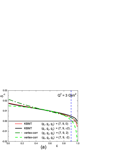
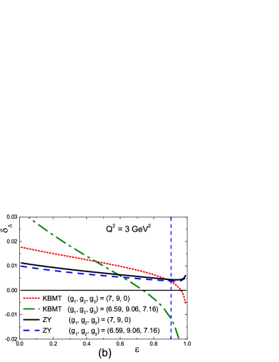
Figure 3: $\delta_{\Delta}$ vs. $\epsilon$ at $Q^{2}=3$ GeV². (a) With $\Delta$ form factors of Eq. (13) and coupling parameters $g_{1}=7,\,g_{2}=9$. The (red) dotted and (black) solid curves correspond to $g_{3}=0$ and $g_{3}=\pm 2$, respectively, using vertex relation of Eq. (9). (Green) dashed and (olive) dash-doted curves correspond to $g_{3}=$ -2 and 2, obtained with the correct vertex relation of Eq. (8). (b) Dependence of $\delta_{\Delta}$ on $\epsilon$ with the use of correct vertex function but different coupling constants and form factors. The (red) dotted and (olive) dash-doted curves, labelled by KBMT correspond to $g_{1}=7,g_{2}=9,g_{3}=0$ and $g_{1}=6.59,g_{2}=9.06,g_{3}=7.16$, respectively, both with the $\Delta$ form factors of Eq. (13) employed in [18]. The (blue) dashed and (black) solid curves, labelled by ZY, correspond to $g_{1}=7,g_{2}=9,g_{3}=0$ and $g_{1}=6.59,g_{2}=9.06,g_{3}=7.16$ with the realistic $\Delta$ form factors of Eq. (LABEL:D3).

Fig. (3b) illustrates the importance of employing realistic $\gamma N\Delta$ form factors and coupling constants, when the correct vertex functions are used. The (red) dotted and olive dash-doted curves, labeled by KBMT, obtained with the $\Delta$ form factors Eq. (13) employed in [18], correspond to $(g_{1}=7,g_{2}=9,g_{3}=0)$ and $(g_{1}=6.59,g_{2}=9.06,g_{3}=7.16)$, respectively. The set of $(g_{1}=6.59,g_{2}=9.06,g_{3}=7.16)$ is the most recent one extracted from experiments [37]. The difference between the dotted and dashed curves arises solely from different values of $g_{3}$ used. The (blue) dashed and (black) solid curves, labeled by ZY and obtained with the realistic $\Delta$ form factors Eq. (LABEL:D3), correspond to $(g_{1}=7,g_{2}=9,g_{3}=0)$ and $(g_{1}=6.59,g_{2}=9.06,g_{3}=7.16)$, respectively. The large differences between (red) dotted and (black) solid curves, and (green) dash-dotted and (blue) dashed curves, are attributed to the different form factors used. However, one notes that the (black) solid and (blue) dashed curves are very close to each other which implies that once the realistic form factors are employed, the effect of Coulomb quadrupole coupling is greatly reduced.

Hereafter, all the results to be given are obtained with the use of correct $\gamma N\Delta$ vertex function, realistic form factors, and coupling constants, unless otherwise specified.

Recently, it has been assumed in [24] that for $s=(p_{1}+p_{2})^{2}\rightarrow\infty$ (Regge limit), which leads to $\epsilon\rightarrow 1$, the TPE correction to $ep$ sccattering amplitude should vanish. The assumption is made so that an unsubtracted fixed-$t$ dispersion relation can be written down for the TPE amplitude. Subsequently, such an assumption has been employed in various analyses [26, 45, 27] to extract TPE corrections from experimental data. Whether such a assumption is valid remains to be substantiated. The calculations of pQCD [30, 29] and SCET [11] do support such an assumption. Nevertheless, it is not clear whether their results would hold up in the soft hadronic scale. In fact, the results of the GPD calculation, shown in Fig. 8 of [21] are not in line with such an assumption, albeit the deviation is small. Our results for TPE-N, which agree with those reported in [17, 19], do possesses this property when monopole form factors are used. However, as seen in Fig. 3, such a feature is not observed in our results for TPE-$\Delta$. They appear to either rise or decrease rapidly as $\epsilon\rightarrow 1$, which look surprising or even "pathological". It is not immediately clear to us why this is so. One possible explanation is that hadronic models such as ours, are not applicable when $s\rightarrow\infty$ and $\epsilon\rightarrow 1$. This is similar to the case that one does not expect the hadronic model to be reliable at large $Q^{2}$. At present, there exists no model calculation which is reliable at all scales. For example, predictions of partonic calculations of [20, 21] are not expected to be reliable for small values of $\epsilon$. In [11], the applicability of SCET is stated to be restricted in the region of $\epsilon_{min}<\epsilon<\epsilon_{max}$, with $\epsilon_{min}\sim 0.42-0.60$ for $Q^{2}\sim 3-6$ GeV². A conservative estimate of the applicability of our hadronic model would be for $W=\sqrt{s}\leq 3-4$ GeV. The corresponding range of $\epsilon$ for $W\sim 3-4$ GeV and $Q^{2}=1-4$ GeV² is depicted in Fig. 4. The vertical dashed line in Fig. 3 correspond to a value of $W=3.5$ GeV, i.e., $\epsilon<0.904$ at $Q^{2}=3$ GeV². Hereafter we will restrict the comparisons of our predictions with the experimental data at low $Q^{2}$ located in this region.

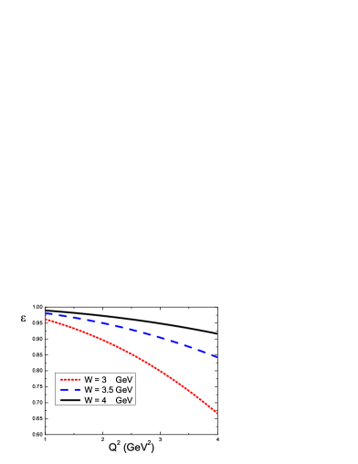
Figure 4: $\epsilon$ vs. $Q^{2}$ for $W\sim 3-4$ GeV.

Contributions of TPE to $\delta$ ’s have also been studied in the dispersion approach of [27, 28]. For the case of the contribution of TPE-N to $\delta_{N}$, our results, which are essentially the same as those obtained in [19], agree well with what are shown in Fig. 5 of [27]. However, for $\delta_{\Delta}$, our results are considerably larger than the corresponding results obtained in [27]. For example, the $\delta_{\Delta}$ ’s at $Q^{2}=3$ GeV² shown by the thick dash-dotted line in Fig. 5 of [27] is only about half of our results. In addition, we further find that $\delta_{\Delta}$ remains substantially smaller than $\delta_{N}$ at large momentum transfer $Q^{2}\sim 6$ GeV² which is at variance with the findings of [28]. The dispersion relation (DR) calculations of [27, 28] for the TPE-$\Delta$ amplitude are based on the following three requirements. Namely, (i) it has no singularities except the branching point at $s=(M_{\Delta}+m_{e})^{2}$, (ii) its branch cut discontinuity is $2iImM^{(\Delta)}$ with $M^{(\Delta)}=M^{(a,\Delta)}+M^{(b,\Delta)}$ as given by Eq. (4), and (iii) it vanishes as $s\rightarrow\infty$. A close look at the amplitude of $M^{(a,\Delta)}$ given in Eq. (4) and the corresponding one for the crossed box diagram, clearly indicates that the requirements of (i) and (ii) are satisfied except the $\Delta$ form factors employed are different from those used in [27, 28], which are not expected to be responsible for the marked difference found in the above. The biggest difference between our calculation and those of [27, 28] most likely lies in condition (iii). This point remains to be further investigated.

3.2 $\Delta(1232)$ contributions to the unpolarized cross section

In this subsection, we will compare our predictions with only two representative sets of data measured in 1994 [46, 12] and 2006 [14], called as data94 and data06, respectively. We do not consider the 1994 data of [47] here as its feature is rather similar to that of data06. The cross section arised from one-photon exchange, $\sigma^{1\gamma}$, will be determined as follows. We first fix the values of $R$ obtained from polarization experiments [1, 2], $R=1-0.13(Q^{2}-0.04)$. As discussed in the last section, TPE corrections to the cross sections are expected to be small and negligible, if not outright vanishing, when $\epsilon\rightarrow 1$. Accordingly, we choose, with the simple least squares method, to fit the experimental reduced cross sections in the $\epsilon>0.7$ region with the OPE expression of Eq. (1) to determine $G_{M}$. It leads to $G_{M}=(0.249,0.146,$ $0.0958,0.0670)$ at $Q^{2}=(1.75,2.5,3.25,4.0)$ GeV², and $G_{M}=(0.964,0.136,$ $0.100,0.0657)$ at $Q^{2}=(0.5,$ $2.64,3.2,4.1)$ GeV², for data94 and data06, respectively. It should be pointed out that the theoretical reduce cross sections are sensitive to the values of $G_{M}$, especially at large $Q^{2}$ region. This is why we retain up to three significant digits in the above expressions. The resulting $\sigma^{1\gamma}$ ^′s, obtained from fitting to the data94 and data06 as explained above and represented by the (olive) dash-dotted curves are shown in Figs. 5 and 6 , respectively.

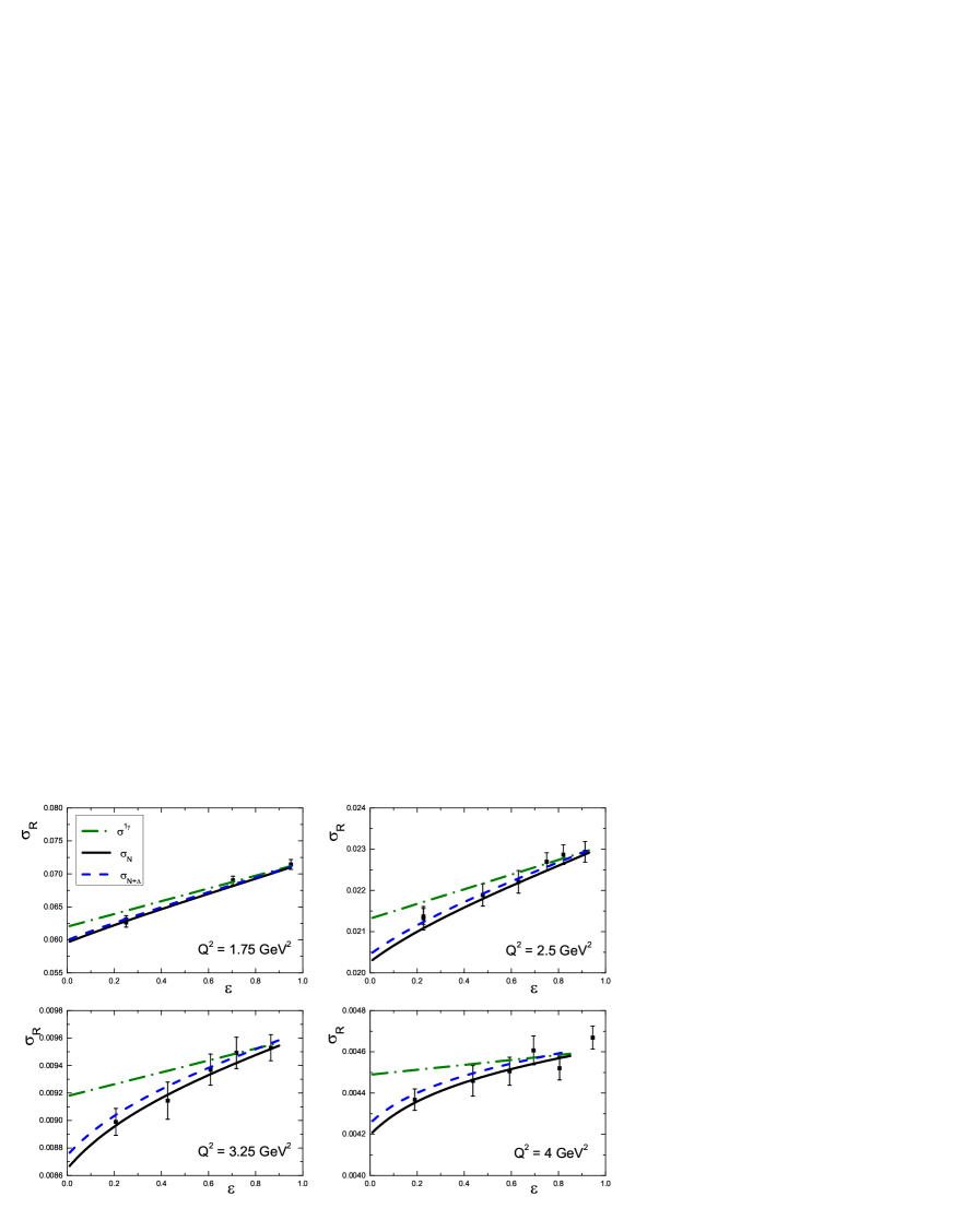
Figure 5: The unpolarized cross section as function of $\epsilon$ at fixed $Q^{2}$. The (olive) dash-dot curves denote the Born cross sections, the (black) solid, and (blue) dashed curves refer to the cross sections including only TPE-N and TPE-N plus TPE-$\Delta$. The theoretical Born cross sections $\sigma^{1\gamma}$ are obtained as explained in the text. Data are from [46].

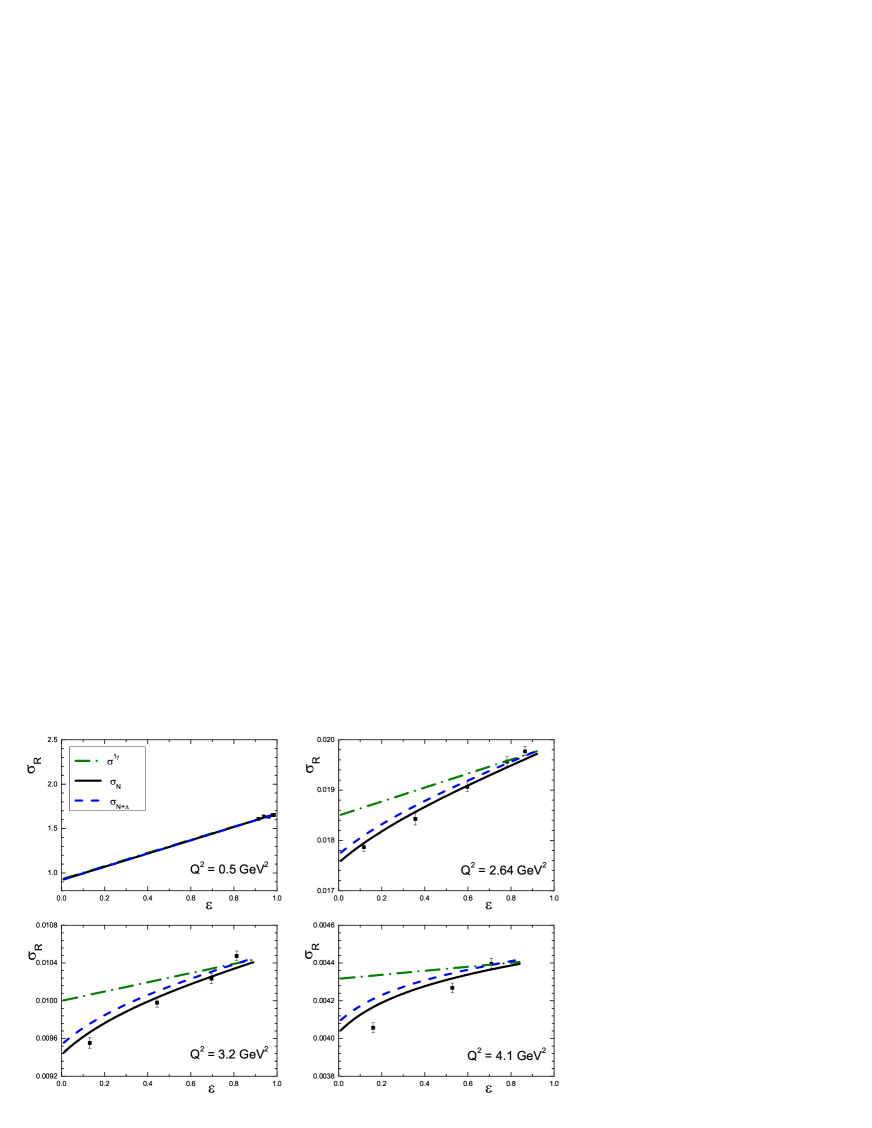
Figure 6: Notations same as in Fig. 5. Data are from [14].

The cross sections including TPE contributions are evaluated as $\sigma^{1\gamma}$ multiplied by the corresponding theoretical TPE corrections via Eqs. (15, 16). We mention that our results including only TPE-N to be presented below are consistent with those obtained in [19]. Note that a different choice of the values for $G_{M}$ will simply shift all three curves shown in each panel of Figs. (5) and (6) by a common factor of $G^{2}_{M}$, since $\bar{\delta}_{N}$ is fairly insensitive to the nucleon form factors as long as they are realistic, as found in Ref. [19].

3.2.1 1994 data set of Andivahis et al.

The unpolarized cross sections of data94 at $Q^{2}=(1.75,2.5,$ $3.25,4.0)$ GeV² are denoted in Fig. 5 by (black) squares. The (black) solid curves, labeled as $\sigma_{N}$, correspond to the predictions including corrections of TPE-N only. It is seen that corrections from TPE-N bring down the predictions of $\sigma^{1\gamma}$ to agree rather well to the data, especially for small $\epsilon$.

Further inclusion of TPE contributions arising from $\Delta$ intermediate states, labeled as $\sigma_{N+\Delta}$, are shown by (blue) dashed curves. The difference between (black) solid and (blue) dashed curves would then represent the contributions of TPE-$\Delta$. The effect of TPE-$\Delta$ clearly is smaller than that of TPE-N and has opposite sign. It is seen that $\sigma_{N+\Delta}$ does not improve the agreement between data and $\sigma_{N}$ except for larger values of $\epsilon$ and $Q^{2}$.

3.2.2 2006 data set of Qattan et al.

The high precision super-Rosenbluth data set data06 are from [14]. The measured unpolarized cross sections at $Q^{2}=0.5,$ $\,2.64,\,3.2,\,4.1$ GeV² are shown in Fig. 6 and denoted by (black) squares. Again the (black) solid curves, labeled as $\sigma_{N}$, correspond to the predictions including corrections of TPE-N only and are seen to bring down the predictions of $\sigma^{1\gamma}$ to agree rather well with the data, especially for small $\epsilon$. In contrast to the case with data94, discrepancy between data and $\sigma_{N}$ begins to develop with increasing $\epsilon$ and higher $Q^{2}$, and becomes substantial for $\epsilon>0.8$ and $Q^{2}>3.2$ GeV².

As with data94, TPE-$\Delta$ contributions are seen to be smaller in magnitude and have opposite sign with TPE-N such that $\sigma_{N+\Delta}$, denoted by (blue) dashed curves in Fig. 6, move $\sigma_{N}$ back toward $\sigma^{1\gamma}$ and the nice agreement between data and $\sigma_{N}$ for $\epsilon<0.7$ and $Q^{2}\leq 3.2$ GeV² is lost. However, for $Q^{2}\geq 3.2$ GeV² and $\epsilon>0.8$, TPE-$\Delta$ actually is beneficial to bridge the difference between data and $\sigma_{N}$.

The discussions presented in the above lead to the following conclusion. Namely, contribution of TPE-$\Delta$ is smaller than that of TPE-N and with opposite sign. For data94, TPE-$\Delta$ contribution, in most cases, brings our model predictions to agree well with the data. For data06, TPE-$\Delta$ contribution is beneficial only in region with larger values of $\epsilon$. However, in the region with small values of $\epsilon$, TPE-$\Delta$ contribution move $\sigma_{N}$ away from the data.

3.2.3 The uncertainties of TPE corrections from $\Delta(1232)$

There are two kinds of uncertainties in the above discussions within our model calculation. The first is from the uncertainties of the input parameters $g_{1},g_{2}$ and $g_{3}$. From Fig. 3(b), we see that the contribution from $g_{3}$ is small, so we will just focus on the uncertainties incurred from $g_{1}$ and $g_{2}$. From Eq. (LABEL:relation-gG), it is seen that the uncertainties of $g_{1}$ and $g_{2}$ are almost equal and proportional to that of $G^{*}_{M}$, since $R_{EM}$ is small in the low $Q^{2}$ region of our interest. The experimental uncertainty of $G^{*}_{M}$ is about $1\%$ . This uncertainty will give rise to an about $2\%$ global uncertainty of the TPE-$\Delta$ corrections $\delta_{\Delta}$, and leads to a correction less than $0.1\%$ to the extracted $R^{\prime}s$.

The second uncertainty is associated with the form factors at finite $Q^{2}$ region. It can be estimated from Figs. 2 and 3(b). In Fig. 2, we see the two form factors (KBMT and ZY) are very different at finite $Q^{2}$, while their TPE corrections shown in Fig. 3(b) are not much different when $g_{3}$ is set to zero. We can hence expect that a $300\%$ difference of $G_{M}^{*}$ at $Q^{2}=3$GeV² will result in $100\%$ difference in the corresponding TPE-$\Delta$ corrections. Since the $G_{M}^{*}$ we use is very close to the experimental one, we expect this uncertainty to be about only at most a few percent. Since the TPE-$\Delta$ corrections are much smaller than TPE-N, this uncertainty will give an even smaller contribution to the uncertainty of the full TPE corrections.

3.3 $\Delta(1232)$ contributions to the extracted $R$ in LT method

We now turn to the correction of TPE to values of $R$ extracted from LT (Rosenbluth) method. In the literature, there are two methods proposed for such a determination. The first one [17] parameterizes $1+\Delta_{un}=a(1+b\epsilon)$ and the corrected $R$ is taken as $\sqrt{R_{0}^{2}-b/B}$ where $R_{0}$ is the extracted $R$ without the inclusion of TPE corrections and $B=1/{\mu_{p}^{2}\tau}$. The second method [48] applies the TPE corrections to the experimental data and then fit the corrected data sets with Eq. (1). Namely, we divide the experimental cross sections by the factor of $(1+\Delta_{un})$ as in Eq. (15) and determine the slope via Eq. (1). We call these two methods as linear parametrization and direct fitting method, respectively. We have applied both methods on the data measured in 1994 [47, 46], which have large error bars, and the data of the recent high-precision super-Rosenbluth experiment [13, 14] measured in 2005 at Jlab. Both methods yield quantitatively similar results. Accordingly, we’ll present only results obtained with the fitting method with data obtained from each single $Q^{2}$ analysis.

Our results for the TPE corrections to the values of $R$ extracted from LT method, with the data of [47, 46] and [14], are presented in Fig. 7, and compared with $R^{\prime}s$ extracted from PT measurements [1, 2, 49] as denoted by open circles and solid squares. The solid triangles, circles, and open rhombi, correspond to the values of $R_{0}$ extracted by the experimentalists which did not include any TPE effects. The (green) stars represent our extracted values of $R$ by fitting method after removing the effects of TPE, including both TPE-N and TPE-$\Delta$, as prescribed by our model where the error bars for $R_{LT,N+\Delta}$ are estimated with only the statistical and point-to-point uncertainty presented in [12, 14] considered. The above comparison for $Q^{2}>4$ GeV² should be taken with caution since our hadronic model calculation might not be reliable in such high $Q^{2}$ region.

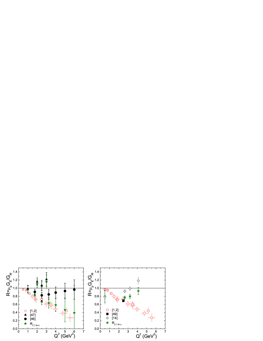
Figure 7: The extracted $R^{\prime}s$ from the LT method after the removal of TPE effects and via direct fitting, are shown by (green) stars and labeled as $R_{LT,N+\Delta}$. Solid triangles, solid circles, and open rhombi denote the values of $R_{0}$ extracted by the experimentalists, i.e., without considering the TPE effects. The PT data are denoted by open circles [1, 2] and solid squares [49]. Left panel: results obtained with the 1994 data of [47, 46]. Right panel: results obtained with the 2006 data of [14].

From the left panel of Fig. 7, we see that the TPE effects prescribed by our model can almost explain the discrepancy in the values of $R$ as extracted from LT and PT methods, as far as only the LT data of [46] are considered. However, substantial discrepancy remains in the case of the LT data of [47, 14] even though the TPE effects do help to explain part of the discrepancy.

From the discussions in the last subsection and here, more cross section experiments will be very helpful to shed light on how to further improve model calculation.

3.4 $\Delta(1232)$ contribution to the ratio $R^{\pm}$ between the positron-proton and electron-proton cross sections

The amplitudes for the positron-proton (${\it e^{+}p}$) and electron-proton (${\it e^{-}p}$) scatterings can be written as $T^{(\pm)}=\pm T_{1\gamma}+T_{2\gamma}$, where $(\pm)$ correspond to the charge of positron and electron, and $T_{1\gamma}$ and $T_{2\gamma}$ denote the scattering amplitudes with $1\gamma$ and $2\gamma$ exchanged, respectively. We then have ratio between the unpolarized cross sections of (${\it e^{+}p}$) and (${\it e^{-}p}$) elastic scattering given as,

$$R^{(\pm)}\equiv\frac{\sigma(e^{+}p)}{\sigma(e^{-}p)}\simeq 1+4Re\left(\frac{T_{2\gamma}}{T_{1\gamma}}\right)=1-2\Delta_{un},$$ (18)

where $\sigma(e^{\pm}p)$ refer to the unpolarized cross sections of $e^{\pm}p$ elastic scatterings. Thus measurements of the ratio of $e^{+}p$ and $e^{-}p$ cross sections provide a direct probe of the real part of the TPE amplitude.

Earlier measurements on $R^{\pm}$, limited by the low intensity of $e^{+}$ beams and hence with large error bars, have been compiled in [50, 9]. Three experiments have recently been undertaken. Two of them have finished data taking [51, 52, 53] with preliminary data published while the third is expected to run soon [54]. In the followings, we will compare our predictions with the published data of [51, 52, 53].

Our predictions for $R^{(\pm)}$, labelled as $N$ and $N+\Delta$ and denoted by (black) solid and (blue) dashed lines, corresponding to results with the contributions of TPE-N and TPE-N plus TPE-$\Delta$ are shown in Fig. 8, respectively, and compared to the preliminary experimental data of VEPP-3 [51, 52]. The open and solid circles denote the data before and after the radiative corrections are applied. In Fig. 8(a) $R^{(\pm)}$ vs. $\epsilon$ at $Q^{2}=1.4$ GeV² is depicted, where the prediction of fit II of a model-independent parametrization of TPE effects in [22], are also shown. We have chosen to present the data and our predictions for $R^{(\pm)}$ vs. $\epsilon$ at fixed $Q^{2}=1.4$, instead of $R^{(\pm)}$ vs. $\epsilon$ at fixed incident electron lab energy $E_{e}=1.6$ GeV as was done in the left panel of Fig. 1 in [51, 52] is because a CLAS experiment at the same $Q^{2}$ has recently finished data taking and being analyzed [55]. Fig. 8(b) shows $R^{\pm}$ vs. $\epsilon$ at incident electron lab energy $E_{e}=1$ GeV.

It is seen in Fig. 8 that, in general, our results for $N+\Delta$ agree with the preliminary data of VEPP-3 well except for the point at $E_{e}=1$ GeV and $\epsilon=0.34\,(Q^{2}=0.90$ GeV${}^{2})$. The inclusion of $\Delta$ in the intermediates states in the TPE diagrams is also seen to somewhat improve the agreement with the data. The effect of TPE associated with $\Delta$ excitation on $R^{\pm}$, though small at large $\epsilon$, becomes substantial at small $\epsilon$. We also find that it is very important to use the correct $\gamma N\Delta$ vertex function as employed in this investigation in this kinematical region.

The good agreement between our prediction and the data for $R^{\pm}$ is encouraging and indicates that the real part of $T_{2\gamma}$ prescribed by our model of TPE might be a reasonable one, at least in the small $Q^{2}$ region.

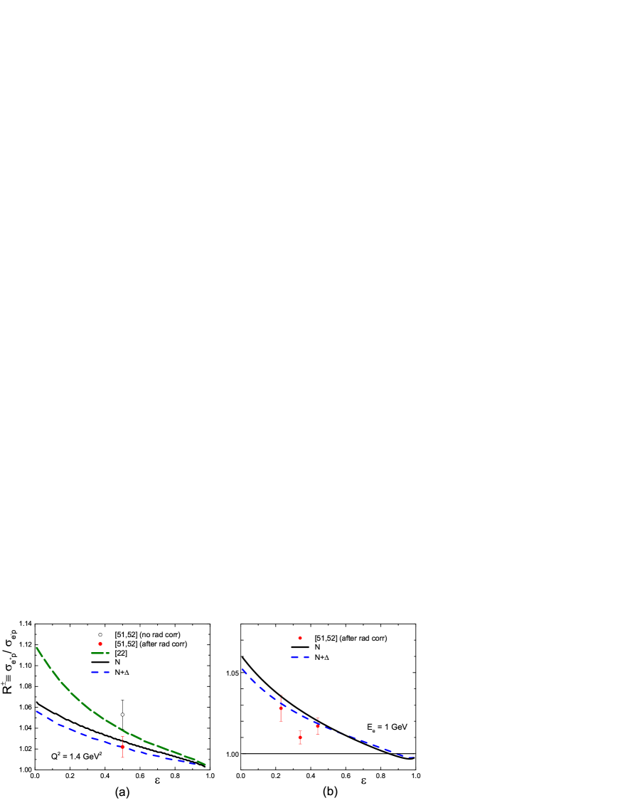
Figure 8: TPE corrections to the ratio $R^{\pm}$. The (black) solid and (blue) dashed curves, refer to predictions with TPE corrections from the $N$ only, and $N+\Delta$ intermediate states included, respectively. The preliminary experimental data are taken from [51, 52], with open and solid circles corresponding to data before and after the radiative corrections are applied. (a) $R^{\pm}$ vs. $\epsilon$ at $Q^{2}=1.4$ GeV². The dash-dotted curve, is the prediction of a model-independent parametrization II of TPE corrections of [22]. (b) $R^{\pm}$ vs. $\epsilon$ at incident electron lab energy $E_{e}=1$ GeV.

We next compare our predictions with the recent CLAS data listed in Table II of [53] at $Q^{2}=0.206$ GeV² as shown in Fig. 9, with the same notation as in Fig. 8. The large luminosity-related systematic uncertainty of 0.05 given there are not included in the figure.

We see considerable discrepancy between our prediction and the data if the large luminosity-related systematic uncertainty is not included. It will be interesting to see whether such discrepancy persists after the large luminosity-related systematic uncertainty is reduced from the experiment. Here we see our prediction with TPE-N approaches one when $\epsilon\rightarrow 1$ as expected from the argument presented at the end of Sec. III-A. The results with TPE-$\Delta$ included, however, do begin to increase near $\epsilon=1$ as hinted by the data. This brings up an interesting question. Namely, whether our results for TPE-$\Delta$ is a realistic one or the uncertainty of the beam luminosity in the experiment of [53] will eventually bring the data down to one near $\epsilon=1$.

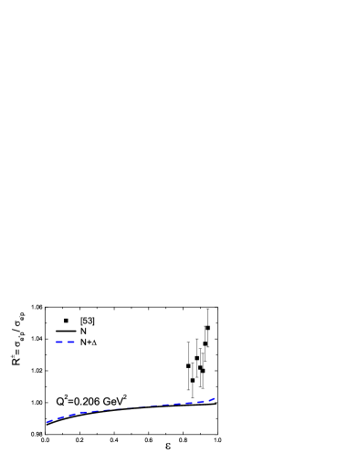
Figure 9: TPE corrections to $R^{\pm}$ at $Q^{2}=0.206$ GeV². Notations same as Fig. 8 and the data are from [53].

3.5 $\Delta$ contribution to the single spin asymmetries $B_{n}$ and $A_{n}$

We now turn to the effect of TPE in the single spin asymmetries $B_{n}$ and $A_{n}$. Since both vanish within OPE approximation because of the time reversal invariance, they provide direct access to the TPE amplitude. However, in contrast to $R^{\pm}$ discussed in the last subsection which probes the real part of $T_{2\gamma}$, $B_{n}$ and $A_{n}$ are related to the imaginary part of the of the TPE amplitude instead.

3.5.1 Beam-normal single spin asymmetries $B_{n}$

For a beam polarized perpendicular to the scattering plane, the single spin asymmetry is defined as

$$B_{n}\equiv\frac{\sigma^{\uparrow}_{e}-\sigma^{\downarrow}_{e}}{\sigma^{\uparrow}_{e}+\sigma^{\downarrow}_{e}},$$ (19)

where $\sigma^{\uparrow}_{e}(\sigma^{\downarrow}_{e})$ denotes the cross section for unpolarized proton target and electron beam spin parallel (antiparallel) to the vector $\hat{n}$ normal to the scattering plane,

$$\hat{n}=\frac{\vec{p}_{1}\times\vec{p}_{3}}{|\vec{p}_{1}\times\vec{p}_{3}|}.$$ (20)

It is a challenging task to measure $B_{n}$ because to polarize an ultrarelativistic electron in the direction normal to its momentum involves a suppression factor of $m_{e}/E_{e}$ which is of the order of $10^{-4}-10^{-3}$ for $E_{e}$ of the order of GeV. This type of difficult experiments [56, 57, 58, 59, 60] have been carried out as by-product of the intensive effort to measure the nucleon strange form factors from the parity-violating asymmetry of the elastic electron-proton scattering [61]. The TPE and $\gamma Z$-exchange corrections to the parity-violating asymmetry have been studied in [62, 63, 39].

As elaborated in [42], the imaginary part of the TPE amplitude can be related, via unitarity, to the doubly virtual Compton scattering tensor on the nucleon with all possible intermediate hadronic states to be on-shell. In [42], they considered only the contributions of $\pi N$ intermediate states by modeling the doubly virtual Compton scattering tensor in terms of the $\gamma^{*}N\rightarrow\pi N$ amplitude. In our calculations of $B_{n}$ and $A_{n}$, we will assume that in the resonance region, $\pi N$ intermediate states are saturated by the excitation of $\Delta$ with a realistic decay width. We follow the recipe of [64] to account for the effect of the $\Delta$ width on $B_{n}$ (and similarly $A_{n}$ in the following subsection) as follows, with the familiar Breit-Wigner form of constant width $\Gamma_{\Delta}=116$ MeV,

$$B_{n} = \int_{M_{\Delta}-2\Gamma_{\Delta}}^{M_{\Delta}+2\Gamma_{\Delta}}B_{n}(M_{D})\rho(M_{D})dM_{D},$$

$$\rho(M_{D}) = -\frac{1}{\pi}Im\left[\frac{2M_{D}}{M_{D}^{2}-M_{\Delta}^{2}+iM_{\Delta}\Gamma_{\Delta}}\right],$$ (21)

where $B_{n}(M_{D})$ is given by Eq. (19) with the mass of $\Delta$, $M_{\Delta}$, replaced by $M_{D}$.

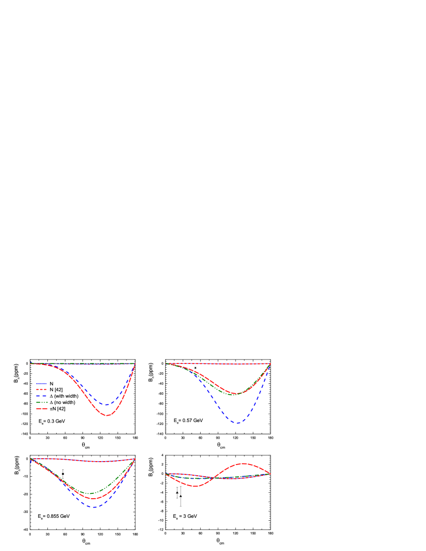
Figure 10: Our predictions for the effects of TPE-N and TPE-$\Delta$, with and without $\Delta$ width, on $B_{n}$ vs. $\theta_{CM}$ at $E_{e}=0.3,0.57,0.855,3\,$GeV as compared with results obtained in [42]. The notation for the various curves are explained in the left top panel. The (red) dot-dashed curves denote the results of [42] with $\pi N$ continuum in the intermediate states. The data are from [57, 59, 60].

Our predictions for $B_{n}$ vs. CM angle $\theta_{cm}$ at four electron energies $E_{e}=0.3,0.57,0.855,3\,$ GeV are presented in Fig. 10 and compared with results obtained in [42], where $\gamma^{*}N\rightarrow\pi N$ amplitude is taken from a phenomenological analysis of electroproduction observables [65]. Both calculations obtain very small contributions from TPE with only nucleon in the intermediate states as indicated by (red) short-dashed and (green) dotted lines, respectively. Our results for contributions from $\Delta$ without and with width are given by (blue) dashed and (green) dot-dot-dashed lines, while the contributions from $\pi N$ intermediate states as estimated by [42] are denoted by (red) dot-dashed lines.

At $E_{e}=0.3\,$GeV in the upper left panel of Fig. 10, it is seen that the contribution from $\Delta(1232)$ intermediate states is zero if $\Delta$ is treated as a stable particle, i.e., with the $\Delta$ width taken to be zero. This can be understood as follows. Namely, $B_{n}$ is related to the imagine parts of the TPE amplitude which would receive contributions only from on-shell intermediate states. For the $e\Delta$ intermediate states, on-shell condition leads to a threshold energy for the electron $E_{e}^{thr}$,

$$E_{e}^{thr}=\frac{M_{\Delta}^{2}-M_{N}^{2}+2M_{\Delta}m_{e}}{2M_{N}}\approx 0.34GeV,$$ (22)

In the calculation of [42], the inelastic intermediate states are taken as $\pi N$ and the on-shell conditions result in a threshold value of $E_{e}^{thr}=0.151$ GeV which is smaller than $0.3$ GeV. This is why [42] would obtain nonvanishing result for $B_{n}$ in the case of $E_{e}=0.3$ GeV, as shown in the upper left panel of Fig. 10. It is seen that the effect of the $\Delta$ width is substantial but begin to decrease as energy increases to pass over the region dominated by the $\Delta$. Note that the vertical scales in the lower two figures are different from the upper two.

For $E_{e}=0.3,0.57,0.855\,$ GeV, our results show similar angular dependence as those obtained in [42] but the absolute magnitude of our result at $E_{e}=0.57\,$ GeV is considerably larger. The two data points at $E_{e}=0.57,0.855\,$GeV come from [57] and their absolute magnitudes are smaller than the predictions of ours and those of [42]. At $E_{e}=3\,$GeV, the absolute magnitudes of our results are much smaller than experimental data [59, 60] and also show very different behavior with the results in [42]. This can be understood naturally as the center of mass energy $\sqrt{s}$ reaches about $4\,$GeV, where the higher resonances, not considered in our model, will dominate.

In Fig. 11, our predictions for the variations of $B_{n}$ w.r.t. electron energy $E_{e}$ at $\theta_{cm}=120^{\circ}$ and $150^{\circ}$ are shown, and compared with the corresponding results of [42], denoted by (red) dashed and (black) dash-dotted lines, respectively, and the experimental data [56, 58, 59, 60]. The kinks seen in our predictions around $\theta_{cm}$ arise from the competition between the contribution of the mass $M_{\Delta}$ and the width $\Gamma_{\Delta}$ as explained earlier. It is interesting to see that our predictions agree with the data better than those of [42] except for one data point at $\theta=120^{\circ}$ with $E_{e}\sim 0.7$ GeV.

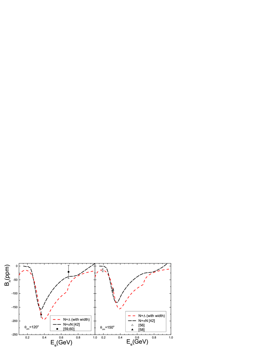
Figure 11: Our predictions for $B_{n}$ vs. $E_{e}$ at $\theta_{cm}=120^{\circ},150^{\circ}$, with contributions coming from nucleon and $\Delta$ together and denoted by (red) dashed lines, are compared with results obtained in [42], as given by (black) dot-dashed lines. The data are from [56, 58, 59, 60].

3.5.2 Target-normal single spin asymmetries $A_{n}$

The target-normal spin asymmetry $A_{n}$ is defined as

$$A_{n}\equiv\frac{\sigma^{\uparrow}_{p}-\sigma^{\downarrow}_{p}}{\sigma^{\uparrow}_{p}+\sigma^{\downarrow}_{p}},$$ (23)

where $\sigma^{\uparrow\downarrow}_{p}$ are the corresponding cross sections of $e(p_{1})$ $p^{\uparrow\downarrow}(p_{2})\rightarrow e(p_{3})p(p_{4})$ with the polarization vector of the target proton normal to the scattering plane. To including the effects from the width of the intermediate $\Delta$ for $A_{n}$, we use similar expression for $B_{n}$ as given in Eq. (21)

$$A_{n} = \int_{M_{\Delta}-2\Gamma_{\Delta}}^{M_{\Delta}+2\Gamma_{\Delta}}A_{n}(M_{D})\rho(M_{D})dM_{D}.$$ (24)

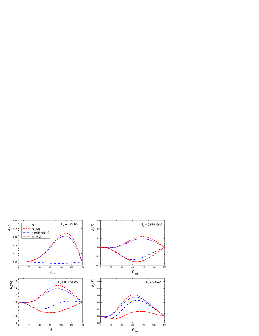
Figure 12: Our predictions for $A_{n}$ vs $\theta_{cm}$ at fixed initial electron $E_{e}=0.2,0.570,0.855,2\,$GeV. Notations same as in Fig. 10. Results from [42] are also shown for comparison.

Fig. 12 shows our predictions for $A_{n}$ vs. $\theta_{cm}$, and compared with the results of [42]. It is seen that the results coming from the nucleon intermediate states are similar angular variation, though differ in magnitudes by $\sim 15\%$. For the inelastic contributions, at $E_{e}=0.2,0.57\,$GeV cases, our results are also very close to those obtained in [42]. However, for $E_{e}=0.855$ and $2$ GeV, our results and those obtained in [42] agree only at the small $\theta_{cm}$ and begin to differ at larger angle, say, for $\theta_{cm}>30^{\circ}$ at $E_{e}=2$ GEV, as in the case of $B_{n}$. The difference lies not only on magnitude but also in angular dependence. It could be attributed to the treatment of the $\Delta$ width and the contributions from higher nucleon resonances.

3.6 $\Delta$ contribution to the polarized variables $P_{t},P_{l},$ and $R_{PT}$

In the last five subsections, we are concerned only with the TPE corrections to the unpolarized observables and single spin asymmetries $A_{n}$ and $B_{n}$. However, since the interest in TPE effects arises from the discrepancy between the values of $R$ extracted from Rosenbluth separation (LT) and polarization transfer (PT) methods, it is hence important that we also study the TPE corrections to the polarization observables $P_{t},P_{l}$.

The TPE corrections to $P_{t},P_{l}$ was studied in a hadronic model in [19]. However, they only considered the correction of TPE arising from $N$ intermediate states. In the followings, we present our predictions for the TPE corrections from both $N$ and $\Delta$ intermediate states to $P_{t},P_{l}$ and compare them with the data of a recent precise measurement carried out at Jefferson Lab in Hall C, in the $\vec{e}+p\rightarrow e+\vec{p}$ elastic scattering [49].

The longitudinal and transverse polarizations of the recoil proton with a longitudinally polarized electron of helicity $\lambda$ are given by

$$\lambda P_{t,l}\equiv\frac{\sigma^{+}_{t,l}(\lambda)-\sigma^{-}_{t,l}(\lambda)}{\sigma^{+}_{t,l}(\lambda)+\sigma^{-}_{t,l}(\lambda)},$$ (25)

where $\sigma^{\pm}_{t,l}(\lambda)$ denote the cross sections of $e(p_{1},s_{1})p(p_{2})\rightarrow e(p_{3})p(p_{4},s_{t,l})$ with $s_{t,l}$ the corresponding transverse and longitudinal polarization vectors (in the scattering plan) of the final proton [66, 67]. Namely, if we denote the spin direction of the recoil proton in its rest frame as $\vec{\zeta}$, then $\vec{\zeta}_{l}\parallel\vec{p}_{4}$ and $\vec{\zeta}_{t}\parallel\hat{x}$, where $\hat{x}=\hat{y}\times\hat{z}$, with unit vectors $\hat{y}$ in the direction of $\vec{p}_{1}\times\vec{p}_{3}$ and $\hat{z}\parallel\vec{p}_{4}$. The superscripts + and - correspond to the cases where $\vec{\zeta}_{l,t}$ are parallel or antiparallel to $\vec{p}_{4}$ and $\hat{x}$, respectively. Note that $P_{t,l}$ is independent of $\lambda$. We can also write

$$\sigma^{\pm}_{t,l}(\lambda)=\frac{1}{2}\sigma_{un}(1\pm\lambda P_{t,l}),$$ (26)

where the unpolarized cross section is given by

$$\sigma_{un} = \frac{1}{2}(\sigma_{t,l}^{+}(+1)+\sigma_{t,l}^{+}(-1)+\sigma_{t,l}^{-}(+1)+\sigma_{t,l}^{-}(-1))$$ (27)

$$= \sigma_{t,l}^{+}(+)+\sigma_{t,l}^{-}(+)$$

$$= \sigma_{t,l}^{+}(-)+\sigma_{t,l}^{-}(-).$$

The second and the third lines in the above equation hold because parity conservation leads to $\sigma_{t,l}^{m}(\lambda)=\sigma_{t,l}^{-m}(-\lambda)$.

In OPE approximation,

$$P_{t}^{1\gamma} = -\frac{1}{\sigma_{R}}\sqrt{\frac{2\epsilon(1-\epsilon)}{\tau}}G_{E}G_{M},$$

$$P_{l}^{1\gamma} = \frac{1}{\sigma_{R}}\sqrt{(1-\epsilon^{2})}G_{M}^{2},$$ (28)

which leads to the well-known result of Eq. (3). The TPE and other higher-order corrections to $P_{t},P_{l}$ and $R_{PT}$ are defined as, in analogous to Eq. (15),

$$P_{t,l}=P_{t,l}^{1\gamma}(1+\delta P_{t,l}),\hskip 28.45274ptR_{PT}=R_{PT}^{1\gamma}(1+\delta R_{PT}),$$ (29)

where $R_{PT}^{1\gamma}\equiv\mu_{p}G_{E}/G_{M}$ would be value of $R_{PT}$ if all higher-order corrections beyond OPE, including TPE, are negligible.

Since we consider here only the higher-order effects up to TPE, we will equate $P_{t,l}=P_{t,l}^{1\gamma+2\gamma}$ and $R_{PT}=R_{PT}^{1\gamma+2\gamma}$, where the superscripts $1\gamma+2\gamma$ refer to $P_{l,t}$’s evaluated within $1\gamma+2\gamma$ approximation. It is straightforward, albeit tedious, to calculate $P_{t,l}^{1\gamma+2\gamma}$ according to either Eq. (25) or Eq. (26). We mention that in the actual calculation, the IR divergences in the $\sigma^{\pm}_{t,l}(\lambda)$’s have been subtracted as done in Ref. [19].

Our results at $Q^{2}=2.49\,$ GeV² for the TPE corrections to $\delta P_{t,l}$ are presented in Fig. 13, where contributions coming from $N$ and $\Delta$ in the intermediate states, are denoted by (black) solid and (blue) dashed lines, respectively, with their sum given by dash-dotted curves. The data for $\delta P_{l}$, normalized at $\epsilon=0.152$ by the experimentalists are from [49]. It is seen that the our predictions for TPE corrections remain small for $\delta P_{l}$ throughout the entire region of $\epsilon$ and fall considerably below the experiment for the two data points at $\epsilon=0.635,0.785$ as shown in Fig. 13(b). For $\delta P_{t}$, the TPE corrections coming from $N$ and $\Delta$ are both small but not negligible at small values of $\epsilon$ as seen in Fig. 13(a), with nucleon contribution larger than that of the $\Delta$. However, both drop quickly for $\epsilon\geq 0.4$.

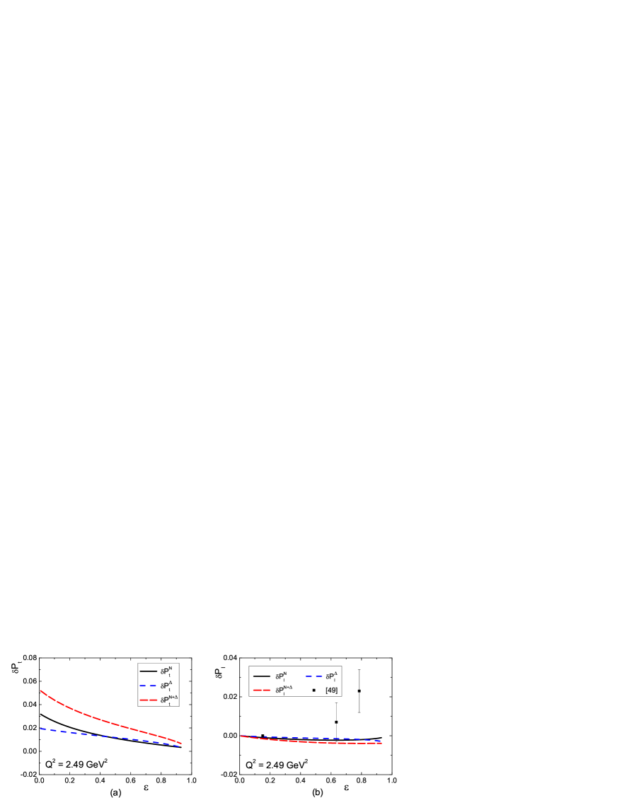
Figure 13: Our predictions of the TPE corrections to $P_{t,l}$. $\delta P^{N}_{t,l}$ and $\delta P^{\Delta}_{t,l}$, denoted by (black) solid and (blue) dashed lines, refer to the corrections arising from $N$ and $\Delta$ in the intermediate states, respectively. The sum is represented by dash-dotted curves and data are from [49] with $\delta P_{l}$ normalized at $\epsilon=0.152$.

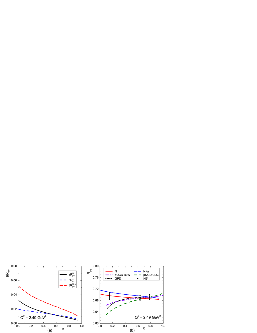
Figure 14: (a) Our predictions for $\delta R_{PT}$ with same notation as in Fig. 13. (b) Our predictions for $R_{PT}$, together with predictions of other theoretical calculations of [21] (partonic) and [30] (pQCD). Data are from [49].

Our results for $\delta R_{PT}$ are shown in Fig. 14 (a) with the same notation as that of Fig. 13. It is easy to see from Eq. (29) that $\delta R_{PT}\simeq\delta P_{t}-\delta P_{l}\simeq\delta P_{t}$ since $\delta P_{l}$ is small. That’s the reason $\delta R_{PT}$ behaves very similar to $\delta P_{t}$ of Fig. 13(a). In Fig. 14 (b), our results for $R_{PT}$ are presented and compared with data of [49], as well as results of other theoretical calculations, including the partonic [21] and pQCD [30] ones. Please note that we have normalized the $R_{PT}^{1\gamma}(1+\delta R_{PT})$ to be equal to $0.692$ at $\epsilon=0.785$ for all model calculations except the (red) solid curve which is normalized with respect to the (blue) dash-dotted curve. This is different from what was done in [49]. It is seen that the prediction of the TPE hadronic model calculation including only the nucleon intermediate states does roughly reproduce the data but adding the effect of the $\Delta$ shifts the curve upward by about $2\%$, whereas all other calculations fail badly, especially at small $\epsilon$ region.

More precision measurements of the polarization transfer observables similar to that of [49] will be most helpful to understand, quantify, and characterize the two-photon-exchange mechanism in electron-proton scattering.

4 Conclusions

We have revisited the question of the contributions of the two-photon exchange associated with the $\Delta$ excitation, to various observables, unpolarized as well as polarized, in the elastic electron-proton scattering, in a hadronic model. Three improvements over previous studies are made in our calculations in order to obtain a better estimate on this important mechanism in the hope of gaining better insight on how to resolve the puzzling discrepancy between the value of $R=\mu_{p}G_{E}/G_{M}$ extracted from LT and PT measurements.

The three improvements are the use of: (1) correct vertex function for $\gamma N\rightarrow\Delta$, as given in Eq. (11); (2) realistic form factors for the $\Delta$; and (3) a realistic set of values for the magnetic dipole, electric quadrupole, and Coulomb quadrupole excitation strength for the $N\rightarrow\Delta$ transition as recently extracted from experiments. We demonstrate by explicit calculations that each of these three improvements incurs considerable change in predictions for the reduced cross sections. We then proceed to calculate, with the three improvements implemented together, the contributions of TPE arising from both nucleon and $\Delta$ intermediate states, to all unpolarized and polarized observables which have been measured or proposed in order to unravel possible causes underlying the discrepancy in the determination of $R$. They include the unpolarized cross sections, extracted value of $R$ in LT method, ratio $R^{\pm}$ between the positron-proton and electron-proton cross sections, beam-normal and target-normal single spin asymmetries, and the transverse and longitudinal polarizations of the recoil proton, $P_{t}$ and $P_{l}$, and their ratio $R_{PT}=-\mu_{p}\sqrt{\tau(1+\epsilon)/2\epsilon}P_{t}/P_{l}$.

For the TPE correction to the unpolarized cross sections associated with the $\Delta$ intermediate states (TPE-$\Delta$), our results for $\delta_{\Delta}$ show a peculiar behavior of rapidly rising or decreasing as $\epsilon\rightarrow 1$. We argue that our hadronic model is not expected to be reliable at large energies and should be restricted for $W\leq 3-4$ GeV. For $W=3.5$ GeV it gives $\epsilon<0.904$ at $Q^{2}=3$ GeV². We hence limit the comparisons of our predictions with the experimental data at low $Q^{2}$ located in this region throughout this study. Moreover, $\delta_{\Delta}$’s we obtain are substantially larger than the DR results of [27, 28]. We speculate that the difference most likely arises from asymptotic behavior of the TPE-$\Delta$ amplitude at $s\rightarrow\infty$ which is assumed to vanish in the DR calculations. Whether the assumption that TPE amplitude would vanish at $\epsilon\rightarrow 1$, i.e., $s\rightarrow\infty$ limit, at soft hadronic scale should be an interesting question to pursue further.

We find that the combined TPE effects of TPE-N and TPE-$\Delta$ as prescribed in our hadronic model, can give a reasonable explanation of the the data measured in 1994 by Andivahis et al. [46]. The values of $R$ extracted from this data set, with TPE effects taken into account, are also close to the PT values. However, this sweet agreement turns sour when the recent high precision super-Rosenbluth data measured at Jlab as well the 1994 data of [47] are analyzed, with TPE effects accounting for less than $50\%$ of the discrepancy between LT and PT values.

The values of the ratio $R^{\pm}$ between $e^{\pm}p$ scatterings predicted by our model, appear to be in reasonable agreement with the preliminary results from VEPP-3 [51, 52], except for one data point. This might indicate that the real part of the amplitude prescribed by our hadronic model is not unsatisfactory, at least in the low $Q^{2}$ region. Better understanding would come only after both VEPP-3 and CLAS [55] finish their analyses as well as more data at higher $Q^{2}$ region. However, our predictions show considerable variance with the data of Moteabbed et al. [53] which were measured at large $\epsilon$. The data seem to remain finite as $\epsilon\rightarrow 1$ which contradicts the general expectation that TPE corrections to $\sigma_{R}$ would approach zero. Whether this is an artifact of the large uncertainty in the beam luminosity in the experiment of [53], or it can be used to support our results that effects of TPE-$\Delta$ for $\sigma_{R}$ show an anomalous behaviour there is real, should be studied further.

For the angular distributions of the beam-normal spin asymmetry $B_{n}$, our predictions are too large at $\theta_{cm}\sim 60^{\circ}$, where there are only two data points available in the energy region in which our model, with only N and $\Delta$ intermediate states included, is expected to be applicable. However, we are encouraged to see that our predictions for the variation of $B_{n}\,\,vs.\,\,E_{e}$, appear to be in satisfactory agreement with data at larger angles $\theta_{cm}\sim 120-150^{\circ}$, except one data point at $E_{e}\sim 0.7$ GeV and $\theta_{cm}\sim 120^{\circ}$. For the target-normal spin asymmetry $A_{n}$, no data are available for comparison. Our results for the angular distributions at lower energies agree, in general, with results of [42]. However, considerable differences, not only in magnitude but also in shape, appear as energy increases. It could arise from the treatment of $\Delta$ width and the contributions of higher nucleon resonances.

For the polarization observables $P_{t},P_{l}$ and the ratio $R_{PT}$, we find that the contribution of TPE-$\Delta$ is smaller than that of TPE-N. Taken together, our hadronic model fails to explain the recent measurement of $P_{l}/P_{l}^{1\gamma}$ by GEP$2\gamma$ at Jlab [49] for $\epsilon>0.6$. Besides, the addition of the effect of TPE-$\Delta$ appears to slightly shift upward by about $2\%$, the reasonable description of the data on $R_{PT}\,\,vs.\,\,\epsilon$ by TPE-N alone.

Several questions have arisen from our study. The first one concerns the large difference in the extracted values of $R$ from data94 of [46] and data06 of [14], both before and after the TPE corrections are implemented. We have little clue about this and experimentalists might be of much help in this regard. Taken together the encouraging results from analyzing data94 and the reasonable agreement found between our predictions for $R^{\pm}$ and the preliminary data from VEPP-3, one is tempted to say that the real part of the amplitude as prescribed from our model might not be very far from realistic, at least in the low $Q^{2}$ region, especially if the further analyses from VEPP-3 and CLAS will confirm our predictions. Our model descriptions of the polarization data of beam-normal asymmetry $B_{n}$ and recoil proton polarizations $P_{l}$ and $R_{PT}$ range from good to poor. The disagreement between our predictions and some of the polarization data raise intriguing challenge to our model. Since the polarization observables like single spin asymmetries are closely connected with the imaginary part of the TPE amplitude, one could immediately ask whether the recipe we follow to account for the effect of the $\Delta$ width is reasonable. In addition, theoretical questions like the off-shell effects of the $\Delta$ and the contributions of the $\pi N$ continuum and higher nucleon resonances which have been studied in [68, 28] also deserve more careful study. Other possible TPE mechanisms, like the t-channel meson exchange processes as suggested in [69], should be explored further as well.

Acknowledgments

We thank J. Arrington, P. G. Blunden, C. W. Kao, and B. Pasquini for helpful communications and discussions. S.N.Y. would like to dedicate this work to the memory of John A. Tjon. This work is supported in part by the National Natural Science Foundations of China under Grant No. 11375044, the Fundamental Research Funds for the Central Universities under Grant No. 2242014R30012 for H.Q.Z. and the National Science Council of the Republic of China (Taiwan) for S.N.Y. under grant No. NSC101-2112-M002-025. H.Q.Z. would also like to gratefully acknowledge the support of the National Center for Theoretical Science (North) of the National Science Council of the Republic of China for his visit in the summer of 2012.

References

- [1] M. K. Jones et al. (JLab Hall A Coll.), Phys. Rev. Lett. 84, 1398 (2000).
- [2] O. Gayou et al. (JLab Hall A Coll.), Phys. Rev. Lett. 88, 092301 (2002).
- [3] A. J. R. Puckett et al., Phys. Rev. Lett. 104, 232401 (2010).
- [4] X. Zhan et al., Phys. Lett. B 705, 59 (2011).
- [5] G. Ron et al., Phys. Rev. C 84, 055204 (2011).
- [6] A. I. Akhiezer, L. N. Rosentsweig and I. M. Shmushkevich, Sov. Phys. JETP. 6, 588 (1958).
- [7] A. I. Akhiezer and M. P. Rekalo, Sov. J. Part. Nucl. 4, 277 (1974).
- [8] C. E. Carlson and M. Vanderhaeghen, Ann. Rev. Nucl. Part. Sci. 57, 171 (2007).
- [9] J. Arrington, P. Blunden P, and W. Melnitchouk, Prog. Nucl. Part. Phys. 66, 782 (2011).
- [10] S. N. Yang, Few-Body Sys. 54, 54 (2013).
- [11] N. Kivel and M. Vanderhaeghen, JHEP 1304, 029 (2013).
- [12] J. Arrington, Phys. Rev. C 68, 034325(2003).
- [13] I. A. Qattan, et al. Phys. Rev. Lett. 94, 142301 (2005).
- [14] I. A. Qattan, Ph.D. thesis, Northwestern University, nucl-ex/0610006.
- [15] L. C. Maximon and J. A. Tjon, Phys. Rev. C 62, 054320 (2000).
- [16] P. A. M. Guichon and M. Vanderhaeghen, Phys. Rev. Lett. 91, 142303 (2003).
- [17] P. G. Blunden, W. Melnitchuk, and J. A. Tjon, Phys. Rev. Lett. 91, 142304 (2003).
- [18] S. Kondratyuk, P.G. Blunden, W. Melnitchuk, and J. A. Tjon, Phys. Rev. Lett. 95, 172503 (2005).
- [19] P. G. Blunden, W. Melnitchuk, and J. A. Tjon, Phys. Rev. C 72, 034612 (2005).
- [20] Y. C. Chen, A. Afanasev, S. J. Brodsky, C. E. Carlson, and M. Vanderhaeghen, Phys. Rev. Lett. 93, 122301 (2004).
- [21] A. Afanasev, S. J. Brodsky, C. E. Carlson, Y. C. Chen, and M. Vanderhaeghen, Phys. Rev. D 72, 013008 (2005).
- [22] Y. C. Chen, C. W. Kao and S. N. Yang, Phys. Lett. B 652, 269 (2007).
- [23] D. Borisyuk and A. Kobushkin, Phys. Rev. C 76, 022201 (2007).
- [24] D. Borisyuk and A. Kobushkin, Phys. Rev. C 78, 025208 (2008).
- [25] D. Borisyuk and A. Kobushkin, Phys. Rev. C 74, 065203 (2006).
- [26] D. Borisyuk and A. Kobushkin, Phys. Rev. C 83, 057501 (2011).
- [27] D. Borisyuk and A. Kobushkin, Phys. Rev. C 86, 055204 (2012).
- [28] D. Borisyuk and A. Kobushkin, Phys. Rev. C 89, 025204 (2014).
- [29] D. Borisyuk and A. Kobushkin, Phys. Rev. C 79, 034001 (2009).
- [30] N. Kivel and M. Vanderhaeghen, Phys. Rev. Lett. 103, 092004 (2009).
- [31] D. Borisyuk and A. Kobushkin, Phys. Rev. C 72, 035207 (2005).
- [32] H. Q. Zhou, C. W. Kao, S. N. Yang, and K. Nagata, Phys. Rev. C 81, 035208 (2010).
- [33] K. Joo et al. (CLAS Collaboration), Phys. Rev. Lett. 88, 122001 (2002).
- [34] N. F. Sparveris et al., Phys. Rev. Lett. 94, 022003 (2005).
- [35] M. Ungaro et al., Phys. Rev. Lett. 97, 112003 (2006).
- [36] C. Alexandrou et al., Phys. Rev. Lett. 94, 021601 (2005).
- [37] V. Pascalutsa, M. Vanderhaeghen, and S. N. Yang, Phys. Repts. 437, 125 (2007).
- [38] J. A. Tjon, P. G. Blunden, and W. Melnitchouk, Phys. Rev. C 79, 055201 (2009).
- [39] K. Nagata, H. Q. Zhou, C. W. Kao, and S. N. Yang, Phys. Rev. C 79, 062051(R) (2009).
- [40] R. Mertig, M. Bohm, and A. Denner, Comput. Phys. Commun. 64, 345 (1991).
- [41] T. Hahn and M. Perez-Victoria, Comput. Phys. Commun. 118, 153 (1999).
- [42] B. Pasquini and M. Vanderhaeghen, Phys. Rev. C 70, 045206 (2004).
- [43] Y. S. Tsai, Phys. Rev. 122, 1898 (1961).
- [44] L. W. Mo and Y. S. Tsai, Rev. Mod. Phys. 41, 205 (1969).
- [45] J. Guttmann, N. Kivel, M. Meziane and M. Vanderhaeghen, Eur. Phys. J. A 47, 77 (2011).
- [46] L. Andivahis et al., Phys. Rev. D 50, 5491 (1994).
- [47] R. C. Walker et al., Phys. Rev. D 49, 5671 (1994).
- [48] J. Arrington, W. Melnitchouk and J. A. Tjon, Phys. Rev. C 76, (2007) 035205.
- [49] M. Meziane et al. (GEp2 Collaboration), Phys. Rev. Lett. 106, 132501 (2011).
- [50] Arrington, Phys. Rev. C 69, 032201 (2004).
- [51] A. V. Gramolin et al., Nucl. Phys. Proc. Suppl. 225-227, 216 (2012).
- [52] D. M. Nikolenko et al., EPJ Web of Conferences 66, 06002 (2014).
- [53] M. Moteabbed et al. (CLAS Coll.), Phys. Rev. C 88, 025210 (2013),
- [54] M. Kohl et al. (OLYMPUS Coll.), EPJ Web Conf. 66, 06009 (2014).
- [55] L. Weinstein, private communication.
- [56] S. P. Wells et al., Phys. Rev. C 63, 064001 (2001).
- [57] F. E. Maas et al. , Phys. Rev. Lett. 94, 082001 (2005).
- [58] L. Capozza, Eur. Phys. J. A 32, 497(2007).
- [59] D. Androic et al. (G0 collaboration), Phys. Rev. Lett. 107, 022501 (2011).
- [60] D. S. Armstrong et al. (G0 collaboration), Phys. Rev. Lett. 99, 092301 (2007).
- [61] D. Androic et al. (G0 collaboration), Phys. Rev. Lett. 104, 012001 (2010) and references contained therein.
- [62] A. V. Afanasev and C. E. Carlson, Phys. Rev. Lett. 94, 212301 (2005).
- [63] H. Q. Zhou, C. W. Kao, and S. N. Yang, Phys. Rev. Lett. 99, 262001 (2007); 100, 059903(E) (2008).
- [64] H. Nagahiro, L. Roca and E. Oset, Phys. Rev. D 77, 034017 (2008).
- [65] L. Tiator, D. Dreschel, O. Hanstein, S. S. Kamalov, and S. N. Yang, Nucl. Phys. A 689, 205c (2001).
- [66] Michail P. Rekalo and E. Tomasi-Gustafsson, arXiv: nucl-th 0202025.
- [67] Glenn A. Ladinsky, Phys. Rev. D. 46, 2922 (1992).
- [68] S. Kondratyuk and P. G. Blunden, Phys.Rev. C 75, 038201 (2007).
- [69] Hong-Yu Chen and Hai-Qing Zhou, Phys.Rev. C 90, 045205 (2014).