Exploration of charmed pentaquarks

Abstract

In this work, we explore the charmed pentaquarks, where the relativistic five-quark equations are obtained by the dispersion relation technique. By solving these equations with the method based on the extraction of the leading singularities of the amplitudes, we predict the mass spectrum of charmed pentaquarks with $J^{P}=1/2^{\pm}$ and $3/2^{\pm}$, which is valuable to further experimental study of charmed pentaquark.

I introduction

Exploring and investigating exotic states, which include glueball, hybrid state and multiquark states, are an intriguing research topic in particle physics. With more and more observations of new hadronic states, there were extensive discussions of whether these observed new hadronic states are good candidates of exotic states (see Refs. 1 ; 2 for a recent review). Studying the hadronic configuration beyond the conventional meson and baryon can make our knowledge of non-perturbative QCD be abundant.

In 2013, the BESIII Collaboration announced the observation of the charged charmonium-like structure $Z_{c}(3900)$ in the $J/\psi^{\pm}$ invariant mass spectrum of $e^{+}e^{-}\to J/\psi\pi^{+}\pi^{-}$ at $\sqrt{s}=4.26$ GeV 3 . $Z_{c}(3900)$ can be a good candidate of the $D\bar{D}^{*}$ molecular state 4 ; 5 , which is as one of the four-quark matters. If four-quark matter is possible existing in nature, we naturally conjecture whether there exist pentaquark states.

In 2003, the $\gamma^{12}C\to K^{+}K^{-}X$ reaction was studied and a peak was found in the $K^{+}n$ invariant mass spectrum around 1540 MeV, which was identified as a signal for a pentaquark with positive strangeness, the “$\Theta^{+}(1540)$” 6 . The unexpected finding lead to a large number of poor statistic experiments where a positive signal was also found, but gradually an equally big number of large statistic experiments showed no evidence for such a peak. A comprehensive review of these developments was done in 7 , where one can see the relevant literature on the subject, as well as in the devoted section of Particle Data Group (PDG) 8 .

Although the signal of $\Theta^{+}(1540)$ was not confirmed in experiment, searching for pentaquark is still an important task 9 . Thus, we need to carry out further theoretical study of pentaquark, which can provide us more abundant information of possible pentaquark. We also notice that most of new hadronic states were observed in the charm-$\tau$ energy region. This fact shows that the charm-$\tau$ energy region should be a suitable platform to study pentaquark. Especially, the $Z_{c}(3900)$ observation boosts our confidence to study heavy flavor pentaqurk again.

In this work, we focus on the charmed pentaquark states with $J^{P}=1/2^{\pm},3/2^{\pm}$, which are composed of a charm antiquark and four light quarks. Firstly, we need to construct relativistic five-quark equations, which contain the $u$, $d$, and $c$ quarks. And then, the masses of these discussed pentaquarks can be determined by the poles of these amplitudes, where the constituent quark involved in our calculation is the color triplet and the quark amplitudes obey the global color symmetry. As the main task of this work, we need to perform the calculation of the pentaquark amplitudes which contain the contribution of four subamplitudes: molecular subamplitude $BM$, $D\bar{q}D$, $Mqqq$ subamplitudes and $Dqq\bar{q}$ subamplitude ($D$ denotes the diquark state, $B$ and $M$ are the baryon and meson states), where the relativistic generalization of five-quark Faddeev-Yakubovsky equations is constructed in the form of the dispersion relation 10 . Finally, we can get the masses of the low-lying charmed pentaquarks, which provide valuable information to further experimental search for these predicted charmed pentaquarks.

Our paper is organized as follows. After this introduction, propose the brief discussion of relativistic Faddeev equations. In Sec. III we represent the five-quark amplitudes relevant to charmed pentaquarks. The numerical results are shown in Sec. IV. The last section is devoted to a summary.

II Brief introduction of relativistic Faddeev equations

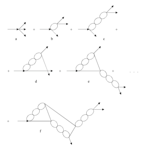
Figure 1: Diagrams which correspond to a) production of three quarks, b-f) subsequent pair interaction.

We consider the derivation of the relativistic generalization of the Faddeev equation for the example of the $\Delta$-isobar ($J^{P}=\frac{3}{2}^{+}$). This is convenient because the spin-flavour part of the wave function of the $\Delta$-isobar contains only nonstrange quarks and pair interactions with the quantum numbers of a $J^{P}=1^{+}$ diquark (in the color state $\bar{3}_{c}$). The $3q$ baryon state $\Delta$ is constructed as color singlet. Suppose that there is a $\Delta$-isobar current which produces three $u$ quarks (Fig. 1a). Successive pair interactions lead to the diagrams shown in Fig. 1b-1f. These diagrams can be grouped according to which of the three quark pairs undergoes the last interaction i.e., the total amplitude can be represented as a sum of diagrams. Taking into account the equality of all pair interactions of nonstrange quarks in the state with $J^{P}=1^{+}$, we obtain the corresponding equation for the amplitudes

$$A_{1}(s,s_{12},s_{13},s_{23})=\lambda+A_{1}(s,s_{12})+A_{1}(s,s_{13})+A_{1}(s,s_{23})\,.$$ (1)

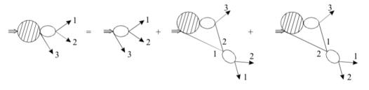
Figure 2: Graphic representation of the equation for the amplitude $A_{1}(s,s_{12})$ (formulae (7) and (11)).

Here the $s_{ik}$ are the pair energies of particles 1, 2 and 3, and $s$ is the total energy of the system. Using the diagrams of Fig. 1, it is easy to write down a graphical equation for the function $A_{1}(s,s_{12})$ (Fig. 2). To write down a concrete equations for the function $A_{1}(s,s_{12})$ we must specify the amplitude of the pair interaction of the quarks. We write the amplitude of the interaction of two quarks in the state $J^{P}=1^{+}$ in the form:

$$a_{1}(s_{12})=\frac{G^{2}_{1}(s_{12})}{1-B_{1}(s_{12})}\,,$$ (2)

$$B_{1}(s_{12})=\int\limits_{4m^{2}}^{\infty}\,\frac{ds^{\prime}_{12}}{\pi}\frac{\rho_{1}(s^{\prime}_{12})G^{2}_{1}(s^{\prime}_{12})}{s^{\prime}_{12}-s_{12}}\,,$$ (3)

$$\rho_{1}(s_{12}) = \left(\frac{1}{3}\,\frac{s_{12}}{4m^{2}}+\frac{1}{6}\right)\left(\frac{s_{12}-4m^{2}}{s_{12}}\right)^{\frac{1}{2}}\,.$$ (4)

Here $G_{1}(s_{12})$ is the vertex function of a diquark with $J^{P}=1^{+}$. $B_{1}(s_{12})$ is the Chew-Mandelstam function 11 and $\rho_{1}(s_{12})$ is the phase spaces for a diquark with $J^{P}=1^{+}$.

The pair quarks amplitudes $qq\to qq$ are calculated in the framework of the dispersion $N/D$ method with the input four-fermion interaction 12 ; 13 with the quantum numbers of the gluon 14 ; 15 .

The four-quark interaction is considered as an input:

$$g_{V}\left(\bar{q}\lambda I_{f}\gamma_{\mu}q\right)^{2}+2\,g^{(s)}_{V}\left(\bar{q}\lambda I_{f}\gamma_{\mu}q\right)\left(\bar{s}\lambda\gamma_{\mu}s\right)+g^{(ss)}_{V}\left(\bar{s}\lambda\gamma_{\mu}s\right)^{2}\,.$$ (5)

Here $I_{f}$ is the unity matrix in the flavour space $(u,d)$. $\lambda$ are the color Gell-Mann matrices. Dimensional constants of the four-fermion interaction $g_{V}$, $g^{(s)}_{V}$ and $g^{(ss)}_{V}$ are parameters of the model. At $g_{V}=g^{(s)}_{V}=g^{(ss)}_{V}$ the flavour $SU(3)_{f}$ symmetry occurs. The strange quark violates the flavour $SU(3)_{f}$ symmetry. In order to avoid additional violation parameters we introduce the scale of the dimensional parameters 15 :

$$g=\frac{m^{2}}{\pi^{2}}g_{V}=\frac{(m+m_{s})^{2}}{4\pi^{2}}g_{V}^{(s)}=\frac{m_{s}^{2}}{\pi^{2}}g_{V}^{(ss)}\,,$$ (6)

$$\Lambda=\frac{4\Lambda(ik)}{(m_{i}+m_{k})^{2}}.$$

Here $m_{i}$ and $m_{k}$ are the quark masses in the intermediate state of the quark loop. Dimensionless parameters $g$ and $\Lambda$ are supposed to be constants which are independent of the quark interaction type. The applicability of Eq. (5) is verified by the success of De Rujula-Georgi-Glashow quark model 14 , where only the short-range part of Breit potential connected with the gluon exchange is responsible for the mass splitting in hadron multiplets.

In the case under discussion the interacting pairs of particles do not form bound states. Therefore, the integration in the dispersion integral (7) run from $4m^{2}$ to $\infty$. The equation corresponding to Fig. 2 can be written in the form:

$$A_{1}(s,s_{12}) = \frac{\lambda_{1}B_{1}(s_{12})}{1-B_{1}(s_{12})}$$ (7)

$$+ \frac{G_{1}(s_{12})}{1-B_{1}(s_{12})}\int\limits_{4m^{2}}^{\infty}\,\frac{ds^{\prime}_{12}}{\pi}\frac{\rho_{1}(s^{\prime}_{12})}{s^{\prime}_{12}-s_{12}}G_{1}(s^{\prime}_{12})$$

$$\times \int\limits_{-1}^{+1}\,\frac{dz}{2}[A_{1}(s,s^{\prime}_{13})+A_{1}(s,s^{\prime}_{23})]\,.$$

In Eq. (7) $z$ is the cosine of the angle between the relative momentum of particles 1 and 2 in the intermediate state and the momentum of the third particle in the final state in the c.m.s. of the particles 1 and 2. In our case of equal mass of the quarks 1, 2 and 3, $s^{\prime}_{13}$ and $s^{\prime}_{12}$ are related by Eq. (8) (See Ref. 16 )

$$s^{\prime}_{13} = 2m^{2}-\frac{(s^{\prime}_{12}+m^{2}-s)}{2}$$

$$\pm \frac{z}{2}\sqrt{\frac{(s^{\prime}_{12}-4m^{2})}{s^{\prime}_{12}}(s^{\prime}_{12}-(\sqrt{s}+m)^{2})(s^{\prime}_{12}-(\sqrt{s}-m)^{2})}\,.$$

The expression for $s^{\prime}_{23}$ is similar to (8) with the replacement $z\to-z$. This makes it possible to replace $[A_{1}(s,s^{\prime}_{13})+A_{1}(s,s^{\prime}_{23})]$ in (7) by $2A_{1}(s,s^{\prime}_{13})$.

From the amplitude $A_{1}(s,s_{12})$ we shall extract the singularities of the diquark amplitude:

$$A_{1}(s,s_{12})=\frac{\alpha_{1}(s,s_{12})B_{1}(s_{12})}{1-B_{1}(s_{12})}\,.$$ (9)

The equation for the reduced amplitude $\alpha_{1}(s,s_{12})$ can be written as

$$\alpha_{1}(s,s_{12}) = \lambda+\frac{1}{B_{1}(s_{12})}\int\limits_{4m^{2}}^{\infty}\,\frac{ds^{\prime}_{12}}{\pi}\frac{\rho_{1}(s^{\prime}_{12})}{s^{\prime}_{12}-s_{12}}G_{1}(s^{\prime}_{12})$$ (10)

$$\times \int\limits_{-1}^{+1}\,\frac{dz}{2}\,\frac{2\alpha_{1}(s,s^{\prime}_{13})B_{1}(s^{\prime}_{13})}{1-B_{1}(s^{\prime}_{13})}\,.$$

The next step is to include into (10) a cutoff at large $s^{\prime}_{12}$. This cutoff is needed to approximate the contribution of the interaction at short distances. In this connection we shall rewrite Eq. (10) as

$$\alpha_{1}(s,s_{12}) = \lambda+\frac{1}{B_{1}(s_{12})}\int\limits_{4m^{2}}^{\infty}\,\frac{ds^{\prime}_{12}}{\pi}\Theta(\Lambda-s^{\prime}_{12})\frac{\rho_{1}(s^{\prime}_{12})}{s^{\prime}_{12}-s_{12}}G_{1}$$ (11)

$$\times \int\limits_{-1}^{+1}\,\frac{dz}{2}\,\frac{2\alpha_{1}(s,s^{\prime}_{13})B_{1}(s^{\prime}_{13})}{1-B_{1}(s^{\prime}_{13})}\,.$$

In Eq. (11) we have chosen a hard cutoff. However, we can also use a soft cutoff, for instance $G_{1}(s^{\prime}_{12})=G_{1}\exp\left(-\frac{(s^{\prime}_{12}-4m^{2})^{2}}{\Lambda^{2}}\right)$, which leaves the results of calculations of the mass spectrum essentially unchanged.

The construction of the approximate solution of Eq. (11) is based on extraction of the leading singularities are close to the region $s_{ik}\approx 4m^{2}$. The structure of the singularities of amplitudes with a different number of rescattering (Fig. 1) is the following 16 . The strongest singularities in $s_{ik}$ arise from pair rescatterings of quarks: square-root singularity corresponding to a threshold and pole singularities corresponding to bound states (on the first sheet in the case of real bound states, and on the second sheet in the case of virtual bound states). The diagrams of Figs. 1b and 1c have only these two-particle singularities. In addition to two-particle singularities diagrams of Figs. 1d and 1e have their own specific triangle singularities. The diagram of Figs. 1f describes a larger number of three-particle singularities. In addition to singularities of triangle type it contains other weaker singularities. Such a classification of singularities makes it possible to search for an approximate solution of Eq. (11), taking into account a definite number of leading singularities and neglecting the weaker ones. We use the approximation in which the singularity corresponding to a single interaction of all three particles, the triangle singularity, is taken into account.

For fixed values of $s$ and $s^{\prime}_{12}$ the integration is carried out over the region of the variable $s^{\prime}_{13}$ corresponding to a physical transition of the current into three quarks (the physical region of Dalitz plot). It is convenient to take the central point of this region, corresponding to $z=0$, to determinate the function $\alpha_{1}(s,s_{12})$ and also the Chew-Mandelstam function $B_{1}(s_{12})$ at the point $s_{12}=s_{0}=\frac{s}{3}+m^{2}$. Then the equation for the $\Delta$ isobar takes the form:

$$\alpha_{1}(s,s_{0})=\lambda+I_{1,1}(s,s_{0})\cdot 2\,\alpha_{1}(s,s_{0})\,,$$ (12)

$$I_{1,1}(s,s_{0})=\int\limits_{4m^{2}}^{\Lambda_{1}}\,\frac{ds^{\prime}_{12}}{\pi}\frac{\rho_{1}(s^{\prime}_{12})}{s^{\prime}_{12}-s_{12}}G_{1}\int\limits_{-1}^{+1}\,\frac{dz}{2}\,\frac{G_{1}}{1-B_{1}(s^{\prime}_{13})}\,.$$ (13)

We can obtain an approximate solution of Eq. (12)

$$\alpha_{1}(s,s_{0})=\lambda[1-2\,I_{1,1}(s,s_{0})]^{-1}\,.$$ (14)

The function $I_{1,1}(s,s_{0})$ takes into account correctly the singularities corresponding to the fact that all propagators of triangle diagrams like those of Figs. 1d and 1e reduce to zero. The right-hand side of Eq. (14) may have a pole in $s$, which corresponds to a bound state of the three quarks. The choice of the cutoff $\Lambda$ makes it possible to fix the value of the mass of the $\Delta$ isobar.

Baryons of $S$-wave multiplets have a completely symmetric spin-flavour part of the wave function, and spin $\frac{3}{2}$ corresponds to the decuplet which has a symmetric flavour part of the wave function. Octet states have spin $\frac{1}{2}$ and a mixed symmetry of the flavour function.

In analogy with the case of the $\Delta$ isobar we can obtain the rescattering amplitudes for all $S$-wave states with $J^{P}=\frac{3}{2}^{+}$, which include quarks of various flavours. These amplitudes will satisfy systems of integral equations. In considering the $J^{P}=\frac{1}{2}^{+}$ octet we must include the interaction of the quarks in the $0^{+}$ and $1^{+}$ states (in the colour state $\bar{3}_{c}$). Including all possible rescattering of each pair of quarks and grouping the terms according to the final states of the particles, we obtain the amplitudes $A_{0}$ and $A_{1}$, which satisfy the corresponding systems of integral equations. If we choose the approximation in which two-particle and triangle singularities are taken into account, and if all functions which depend on the physical region of the Dalitz plot, the problem of solving the system of integral equations reduces to one of solving simple algebraic equations.

In our calculation the quark masses $m_{u}=m_{d}=m$ and $m_{s}$ are not uniquely determined. In order to fix $m$ and $m_{s}$ anyhow, we make the simple assumption that $m=\frac{1}{3}m_{\Delta}(1232)$ $m=\frac{1}{3}m_{\Omega}(1672)$. The strange quark breaks the flavour $SU(3)_{f}$ symmetry (6).

In Ref. 17 we consider two versions of calculations. If the first version the $SU(3)_{f}$ symmetry is broken by the scale shift of the dimensional parameters. A single cutoff parameter in pair energy is introduced for all diquark states $\lambda_{1}=12.2$.

In the Table I the calculated masses of the $S$-wave baryons are shown 17 . In the first version we use only three parameters: the subenergy cutoff $\lambda$ and the vertex function $g_{0}$, $g_{1}$, which corresponds to the quark-quark interaction in $0^{+}$ and $1^{+}$ states. In this case the mass values of strange baryons with $J^{P}=\frac{1}{2}^{+}$ are less than the experimental ones. This means that the contribution color-magnetic interaction is too large. In the second version we introduce four parameters: cutoff $\lambda_{0}$, $\lambda_{1}$ and the vertex function $g_{0}$, $g_{1}$. We decrease the color-magnetic interaction in $0^{+}$ strange channels and calculated mass values of two baryonic multiplets $J^{P}=\frac{1}{2}^{+}$, $\frac{3}{2}^{+}$ are in good agreement with the experimental data 8 .

The essential difference between $\Sigma$ and $\Lambda$ is the spin of the lighter diquark. The model explains both the sign and magnitude of this mass splitting.

The suggested method of the approximate solution of the relativistic three-quark equations allows us to calculate the $S$-wave baryons mass spectrum. The interaction constants, determined the baryons spectrum in our model, are similar to ones in the bootstrap quark model of $S$-wave mesons 15 . The diquark interaction forces are defined by the gluon exchange. The relative contribution of the instanton-induced interaction is less than that with the gluon exchange. This is the consequence of $1/N_{c}$-expansion 15 .

The gluon exchange corresponds to the color-magnetic interaction, which is responsible for the spin-spin splitting in the hadron models. The sign of the color-magnetic term is such as to made any baryon of spin $\frac{3}{2}$ heavier than its spin-$\frac{1}{2}$ counterpart (containing the same flavours).

Table 1: Baryon masses $M(J^{p})$ (GeV). Version 1 (the cutoff parameter $\lambda_{1}=12.2$), version 2 ($\lambda_{0}=9.7$, $\lambda_{1}=12.2$). The vertex functions $g_{0}=0.702$, $g_{1}=0.540$. Experimental values of the baryon masses 8 are given in the parentheses.

	$M(\frac{1}{2}^{+})$			$M(\frac{3}{2}^{+})$
$N$	$0.940$ $0.940$	$(0.940)$	$\Delta$	$1.232$ $1.232$	$(1.232)$
$\Lambda$	$1.022$ $1.098$	$(1.116)$	$\Sigma^{*}$	$1.377$ $1.377$	$(1.385)$
$\Sigma$	$1.050$ $1.193$	$(1.193)$	$\Xi^{*}$	$1.524$ $1.524$	$(1.530)$
$\Xi$	$1.162$ $1.325$	$(1.315)$	$\Omega$	$1.672$ $1.672$	$(1.672)$

III Five-quark amplitudes for the charmed pentaquarks

In the following, we introduce how to get the relativistic five-quark amplitudes for the charmed pentaquarks, where we adopt the dispersion relation technique. Due to the rules of $1/N_{c}$ expansion 18 ; 19 ; 20 , we only need to consider planar diagrams, while the other diagrams can be neglected. By summing over all possible subamplitudes which correspond to the division of complete system into subsystems smaller number of particles, we can obtain the total amplitude.

In general, a five-particle amplitude ($\mathcal{A}$) can be expressed as the sum of ten subamplitudes ($\mathcal{A}_{ij}$ ($i=1,2,3,4$, $j=1,2,3,4,5$)), i.e.,

$$\mathcal{A} = \mathcal{A}_{12}+\mathcal{A}_{13}+\mathcal{A}_{14}+\mathcal{A}_{15}+\mathcal{A}_{23}+\mathcal{A}_{24}$$

$$+\mathcal{A}_{25}+\mathcal{A}_{34}+\mathcal{A}_{35}+\mathcal{A}_{45},$$

where $\mathcal{A}_{ij}$ denotes the subamplitude from the pair interaction of particles $i$ and $j$ in a five-particle system.

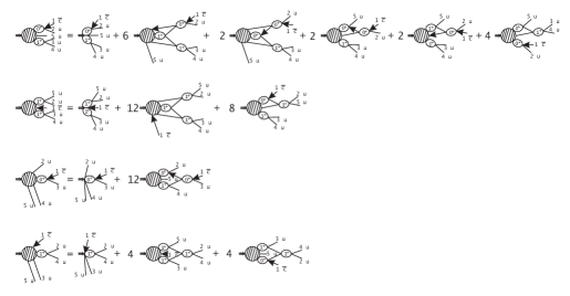
Figure 3: The graphic representation of the equations for the five-quark subamplitudes $A_{k}$ ($k$=1-4) in the case of the $uuuu\bar{c}$ system. Here, we mark $\bar{c}$ and other four light quarks by lines with and without arrow, respectively.

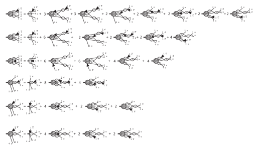
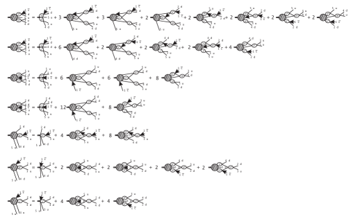
Figure 4: The graphic representation of the equations for the five-quark subamplitudes for the $uuud\bar{c}$ and $udud\bar{c}$ systems. Here, the $\bar{c}$ quark is denoted by the lines with arrow. There are six and seven diagrams for the $uuud\bar{c}$ and $udud\bar{c}$ systems, respectively.

For the sake of simplifying the calculation, we take the relativistic generalization of the Faddeev-Yakubovsky approach. With the $uuuu\bar{c}$ system as an example, we introduce how to obtain $\mathcal{A}_{12}$. Firstly, we need to construct the five-quark amplitude of the $uuuu\bar{c}$ system, where only pair interaction with the quantum numbers of a $J^{P}=1^{+}$ diquark is included. Then, the set of diagrams relevant to the amplitude $\mathcal{A}_{12}$ can further be broken down into groups corresponding to amplitudes: $A_{1}(s,s_{1234},s_{12},s_{34})$, $A_{2}(s,s_{1234},s_{25},s_{34})$, $A_{3}(s,s_{1234},s_{13},s_{134})$, $A_{4}(s,s_{1234},s_{24},s_{234})$, which are shown in Fig. 3 by the graphic representation of the equations for the five-quark subamplitudes. Similarly, we also give the corresponding graphic representation for the $uuud\bar{c}$ and $udud\bar{c}$ systems, which are shown in Fig. 4. For the cases of the $uuud\bar{c}$ and $udud\bar{c}$ systems, there are six and seven subamplitudes, respectively. Here, the coefficients can be obtained by the permutation of quarks 21 ; 22 .

In the following, we need to further illustrate how to write out the subamplitudes $A_{1}(s,s_{1234},s_{12},s_{34})$, $A_{2}(s,s_{1234},s_{25},s_{34})$, $A_{3}(s,s_{1234},s_{13},s_{134})$, and $A_{4}(s,s_{1234},s_{24},s_{234})$, which are in the form of a dispersion relation. Firstly, we need to define the amplitudes of quark-quark and quark-antiquark interaction $a_{n}(s_{ik})$. With the help of four-fermion interaction with quantum numbers of the gluon 15 , we can calculate the amplitudes $q\bar{q}\to q\bar{q}$ and $qq\to qq$ through the dispersion $N/D$ method. Thus, the pair quarks amplitude can be expressed as 15

$$a_{n}(s_{ik}) = \frac{G_{n}^{2}(s_{ik})}{1-B_{n}(s_{ik})},$$

$$B_{n}(s_{ik}) = \int_{(m_{1}+m_{2})^{2}}^{\Lambda_{n}}\frac{ds_{ik}^{\prime}}{\pi}\frac{\rho_{n}(s_{ik}^{\prime})G_{n}^{2}(s_{ik}^{\prime})}{s_{ik}^{\prime}-s_{ik}},$$

where $s_{ik}$ denotes the two-particle subenergy squared. And $s_{ijk}$ is the energy squared of particles $i$, $j$, $k$ while $s_{ijkl}$ is the four-particle subenergy squared. In addition, we also define $s$ as the system total energy squared.

We obtain the concrete forms of $A_{i}$ ($i=1,2,3,4$), i.e.,

$$A_{1}(s,s_{1234},s_{12},s_{34})$$

$$=\frac{\lambda_{1}B_{3}(s_{12})B_{2}(s_{34})}{[1-B_{3}(s_{12})][1-B_{2}(s_{34})]}+6\hat{J}_{2}(3,2)A_{4}(s,s_{1234},s_{23}^{\prime},s_{234}^{\prime})$$

$$\quad+2\hat{J}_{2}(3,2)A_{3}(s,s_{1234},s_{13}^{\prime},s_{134}^{\prime})+2\hat{J}_{1}(3)A_{3}(s,s_{1234},s_{15}^{\prime},s_{125})$$

$$\quad+2\hat{J}_{1}(2)A_{4}(s,s_{1234},s_{25}^{\prime},s_{125})+4\hat{J}_{1}(2)A_{4}(s,s_{1234},s_{35}^{\prime},s_{345}),$$

(15)

$$A_{2}(s,s_{1234},s_{25},s_{34})$$

$$=\frac{\lambda_{2}B_{2}(s_{25})B_{2}(s_{34})}{[1-B_{2}(s_{25})][1-B_{2}(s_{34})]}+12\hat{J}_{2}(2,2)A_{4}(s,s_{1234},s_{23}^{\prime},s_{234}^{\prime})$$

$$\quad+8\hat{J}_{1}(2)A_{3}(s,s_{1234},s_{25}^{\prime},s_{125}),$$ (16)

$$A_{3}(s,s_{1234},s_{13},s_{134})$$

$$=\frac{\lambda_{3}B_{3}(s_{12})}{1-B_{3}(s_{12})}+12\hat{J}_{3}(3)A_{1}(s,s_{1234},s_{12}^{\prime},s_{34}^{\prime}),$$ (17)

$$A_{4}(s,s_{1234},s_{24},s_{234})$$

$$=\frac{\lambda_{4}B_{2}(s_{24})}{1-B_{2}(s_{24})}+4\hat{J}_{3}(2)A_{2}(s,s_{1234},s_{25}^{\prime},s_{34}^{\prime})$$

$$\quad+4\hat{J}_{3}(2)A_{1}(s,s_{1234},s_{12}^{\prime},s_{34}^{\prime}),$$ (18)

where $\lambda_{i}$ denotes the current constants. In addition, the integral operators $\hat{J}_{1}(l)$, $\hat{J}_{2}(l,p)$, and $\hat{J}_{3}(l,p)$ are introduced, where their expressions can be found in Appendix. Taking the same treatment as that given in Ref. 23 , where we pass from the integration over the cosines of the angles to the integration over the subenergies, we can extract two-particle singularities in the amplitudes $A_{1}(s,s_{1234},s_{12},s_{34})$, $A_{2}(s,s_{1234},s_{25},s_{34})$, $A_{3}(s,s_{1234},s_{13},s_{134})$, and $A_{4}(s,s_{1234},s_{24},s_{234})$:

$$A_{1}(s,s_{1234},s_{12},s_{34}) = \frac{\alpha_{1}(s,s_{1234},s_{12},s_{34})B_{3}(s_{12})B_{2}(s_{34})}{[1-B_{3}(s_{12})][1-B_{2}(s_{34})]},$$

$$A_{2}(s,s_{1234},s_{25},s_{34}) = \frac{\alpha_{2}(s,s_{1234},s_{25},s_{34})B_{2}(s_{25})B_{2}(s_{34})}{[1-B_{2}(s_{25})][1-B_{2}(s_{34})]},$$

$$A_{3}(s,s_{1234},s_{13},s_{134}) = \frac{\alpha_{3}(s,s_{1234},s_{13},s_{134})B_{3}(s_{13})}{1-B_{3}(s_{13})},$$

$$A_{4}(s,s_{1234},s_{24},s_{234}) = \frac{\alpha_{4}(s,s_{1234},s_{24},s_{234})B_{2}(s_{24})}{1-B_{2}(s_{24})}.$$

Here, we want to further specify that we do not extract the three-particle and four-particle singularities, which are weaker than the two-particle singularities. In addition, we also adopt the classification of singularities suggested in Ref. 16 . The main singularities in $s_{ik}=(m_{i}+m_{k})^{2}$ there are from pair rescattering of particles $i$ and $k$. First of all, they are threshold square-root singularities. Also possible are singularities which correspond to the bound states. We have apart from two-particle singularities the triangular singularities, the singularities defining the interaction of four and five particles. Such classification allows us to search the corresponding solution by taking into account some definite number of leading singularities and neglecting all the weaker ones. We consider the approximation which defines two-particle, three-, four-, and five-particle singularities. As the smooth functions of $s_{ik}$, $s_{ijk}$, $s_{ijkl}$, and $s$, $\alpha_{1}(s,s_{1234},s_{12},s_{34})$, $\alpha_{2}(s,s_{1234},s_{25},s_{34})$, $\alpha_{3}(s,s_{1234},s_{13},s_{134})$ and $\alpha_{4}(s,s_{1234},s_{24},s_{234})$ can be expanded in a series in the singularity point, where only the first term of this series should be employed further. Thus, we further define the reduced amplitudes $\alpha_{1}$, $\alpha_{2}$, $\alpha_{3}$, $\alpha_{4}$, and the B-functions in the middle point of the physical region of Dalitz-plot at the point $s_{0}$, i.e.,

$$s_{0}^{ik} = {s_{0}}=\frac{s+3\sum_{i=1}^{5}m_{i}^{2}}{0.25\sum_{i,k=1,i\neq k}^{5}(m_{i}+m_{k})^{2}},$$ (19)

$$s_{123} = 0.25s_{0}\sum_{i,k=1,i\neq k}^{3}(m_{i}+m_{k})^{2}-\sum_{i=1}^{3}m_{i}^{2},$$ (20)

$$s_{1234} = 0.25s_{0}\sum_{i,k=1,i\neq k}^{4}(m_{i}+m_{k})^{2}-2\sum_{i=1}^{4}m_{i}^{2}.$$ (21)

Then, we replace the integral Eqs. (15)-(18) corresponding to the diagrams in Fig. 3 by the following algebraic equations

$$\alpha_{1} = \lambda_{1}+6\alpha_{4}J_{2}(3,2,2)+2\alpha_{3}J_{2}(3,2,3)+2\alpha_{3}J_{1}(3,3)$$ (22)

$$+2\alpha_{4}J_{1}(3,2)+4\alpha_{4}J_{1}(2,2),$$

$$\alpha_{2} = \lambda_{2}+12\alpha_{4}J_{2}(2,2,2)+8\alpha_{3}J_{1}(2,3),$$ (23)

$$\alpha_{3} = \lambda_{3}+12\alpha_{1}J_{3}(3,3,2),$$ (24)

$$\alpha_{4} = \lambda_{4}+4\alpha_{2}J_{3}(2,2,2)+4\alpha_{1}J_{3}(2,2,3),$$ (25)

respectively. Here, the definitions of the functions $J_{1}(l,p)$, $J_{2}(l,p,r)$, $J_{3}(l,p,r)$ ($l,p,r$= 1, 2, 3) are listed in Appendix.

Finally, we have the function like

$$\alpha_{i}(s)=F_{i}(s,\lambda_{i})/D(s),$$ (26)

where the masses of these discussed systems can be determined by zeros of $D(s)$ determinants. And, $F_{i}(s,\lambda_{i})$ denotes the function of $s$ and $\lambda_{i}$, which determines the contribution of subamplitude.

IV Numerical results

In Sec. III, the involved parameters in our model include quark masses $m_{u,d}=439$ MeV and $m_{c}=1640$ MeV, where we effectively take into account the contribution of the confinement potential in obtaining the spectrum of charmed pentaquarks. The adopted value of cutoff $\Lambda=10$, which coincides with that taken in Ref. 24 ; 25 . In addition, a dimensionless parameter $g$, which is the gluon coupling constant, is introduced in our calculation. We notice that the mass of charmed pentaquark with both configuration $D_{2}^{*}N$ ($udud\bar{c}$) and quantum number $(I)J^{P}=(0)\frac{3}{2}^{+}$ was calculated through the one-boson-exchange model in Ref. 26 , where its mass is $3387$ MeV. Thus, by reproducing this value in our model, we can determine $g=0.825$, which is adopted in the following calculation to give more predictions of the masses of charmed pentaquarks.

With the above preparation, in this section we present the numerical results of the mass spectrum of the discussed charmed pentaquarks, where the poles of the reduced amplitudes $\alpha_{1}$, $\alpha_{2}$, $\alpha_{3}$, $\alpha_{4}$ correspond to the bound states of charmed pentaquarks. The predicted masses of charmed pentaquarks are shown in Table 2.

Table 2: The obtained low-lying charmed pentaquark masses. Here, the parameters involved in our model include: quark mass $m_{u,d}$ = 439 MeV, $m_{c}$ = 1640 MeV; cutoff parameter $\lambda$ = 10; and gluon coupling constant $g$ = 0.825. Here, – denotes that there does not exist the corresponding charmed pentaquark state.

	$J^{P}$
States	$\frac{1}{2}^{+}$	$\frac{3}{2}^{+}$	$\frac{1}{2}^{-}$	$\frac{3}{2}^{-}$
$\Theta_{c}^{++}(uuuu\bar{c})/\Theta_{c}^{--}(dddd\bar{c})$	3323	3323	3339	3339
$\Theta_{c}^{+}(uuud\bar{c})/\Theta_{c}^{-}(dddu\bar{c})$	2986	3209	3277	–
$\Theta_{c}^{0}(udud\bar{c})$	2980	3387	3280	–

V Summary

As an interesting research reach topic, exploring the exotic multiquark matter beyond conventional meson and baryon is an exciting and important task, which will be helpful to understand the non-perturbative behavior of quantum chromodynamics. The new observation of numerous $XYZ$ particles opens the Pandora’s Box of studying the exotic multiquark matter 2 .

In this work, we studied the charmed pentaquarks with $J^{P}=1/2^{\pm},3/2^{\pm}$ by the relativistic five-quark model, where the Faddeev-Yakubovsky type approach is adopted. The masses of the low-lying charmed pentaquarks are calculated. This information is useful to further experimental search for them in future.

We used some approximations for the calculation of the five-quark amplitude. The estimation of the theoretical error on the pentaquark masses is about 20%. It is usual for model estimations. This result was obtained by the choice of model parameters: gluon coupling constant $g=0.825$ and cutoff parameter $\lambda=10$.

We also notice that there were several experimental efforts on the search for the charmed pentaquarks 27 ; 28 ; 29 , where the present experiment still did not find the evidence of charmed pentaquark. Unlike the mesons, all half-integral spin and parity quantum numbers are allowed in the baryon sector, which means that there exists the mixing between charmed pentaquark and conventional charmed baryon, so that experimentally searching for such charmed pentaquark is not a simple task. In addition, the charmed pentaquarks have the abnormally small widths since the observed charmed pentaquarks with the isospin $I=0,1,2$ and the spin-parity $J^{P}=\frac{1}{2}^{+}$, $\frac{3}{2}^{+}$ are below the thresholds. These facts make the identification of a pentaquark be difficult in experiment.

In summary, exploring the charmed pentaquark is a reach field full of challenges and opportunities. More theoretical and experimental united efforts should be made in the future to establish charmed exotic pentaquark family.

Appendix: Some useful formulae

The definitions of $\hat{J}_{1}(l)$, $\hat{J}_{2}(l,p)$ and $\hat{J}_{3}(l,p)$ are given by

$$\hat{J}_{1}(l)$$

$$=\frac{G_{l}(s_{12})}{[1-B_{l}(s_{12})]}\int_{(m_{1}+m_{2})^{2}}^{\Lambda_{l}}\frac{ds_{12}^{\prime}}{\pi}\frac{G_{l}(s_{12}^{\prime})\rho_{l}(s_{12}^{\prime})}{s_{12}^{\prime}-s_{12}}\int_{-1}^{+1}\frac{dz_{1}}{2},$$

(27)

$$\hat{J}_{2}(l,p)$$

$$=\frac{G_{l}(s_{12})G_{p}(s_{34})}{[1-B_{l}(s_{12})][1-B_{p}(s_{34})]}\int_{(m_{1}+m_{2})^{2}}^{\Lambda_{l}}\frac{ds_{12}^{\prime}}{\pi}$$

$$\quad\times\frac{G_{l}(s_{12}^{\prime})\rho_{l}(s_{12}^{\prime})}{s_{12}^{\prime}-s_{12}}\int_{(m_{3}+m_{4})^{2}}^{\Lambda_{p}}\frac{ds_{34}^{\prime}}{\pi}\frac{G_{p}(s_{34}^{\prime})\rho_{p}(s_{34}^{\prime})}{s_{34}^{\prime}-s_{34}}$$

$$\quad\times\int_{-1}^{+1}\frac{dz_{3}}{2}\int_{-1}^{+1}\frac{dz_{4}}{2},$$ (28)

$$\hat{J}_{3}(l)$$

$$=\frac{G_{l}(s_{12},\widetilde{\Lambda})}{1-B_{l}(s_{12},\widetilde{\Lambda})}\times\frac{1}{4\pi}\int_{(m_{1}+m_{2})^{2}}^{\widetilde{\Lambda}}\frac{ds_{12}^{\prime}}{\pi}\frac{G_{l}(s_{12}^{\prime},\widetilde{\Lambda})\rho_{l}(s_{12}^{\prime})}{s_{12}^{\prime}-s_{12}}$$

$$\quad\times\int_{-1}^{+1}\frac{dz_{1}}{2}\int_{-1}^{+1}dz\int_{-1}^{+1}dz_{2}$$

$$\quad\times\frac{1}{\sqrt{1-z^{2}-z_{1}^{2}-z_{2}^{2}+2zz_{1}z_{2}}},$$ (29)

respectively, where $l,p$ are taken as 1, 2, 3. And $m_{i}$ denotes the corresponding quark mass. In Eqs. (27) and (29), $z_{1}$ is the cosine of the angle between the relative momentum of the particles 1 and 2 in the intermediate state and the momentum of the particle 3 in the final state, taken in the c.m. of particles 1 and 2. In Eq. (29), we can define $z$ as the cosine of the angle between the momenta of the particles 3 and 4 in the final state, taken in the c.m. of particles 1 and 2. $z_{2}$ is the cosine of the angle between the relative momentum of particles 1 and 2 in the intermediate state and the momentum of the particle 4 in the final state, is taken in the c.m. of particles 1 and 2. In Eq. (28), $z_{3}$ is the cosine of the angle between relative momentum of particles 1 and 2 in the intermediate state and the relative momentum of particles 3 and 4 in the intermediate state, taken in the c.m. of particles 1 and 2. $z_{4}$ is the cosine of the angle between the relative momentum of the particles 3 and 4 in the intermediate state and that of the momentum of the particle 1 in the intermediate state, taken in the c.m. of particles 3 and 4.

In Eqs. (27) – (29), $G_{n}(s_{ik})$ denote the quark-quark and quark-antiquark vertex functions, where the concrete expressions of $G_{n}(s_{ik})$ are listed in Table. 3. The vertex functions satisfy the Fierz relations. All of these vertex functions are generated from $g_{V}$, $g_{V}^{(c)}$. Dimensional constants of the four-fermion interaction $g_{V}$, $g_{V}^{(c)}$ are parameters of model. In order to avoid additional violation parameters we introduce the scale of the dimensional parameters similar to (6). Dimensionless parameters $g$ and $\Lambda$ are supposed to be constants which independent of the quark interaction type.

Table 3: The expressions of vertex function $G_{n}(s_{ik})$.

$J^{PC}$	$G_{n}^{2}$
$0^{+}(n=1)$	$4g/3-2g(m_{i}+m_{k})^{2}/(3s_{ik})$
$1^{+}(n=2)$	$2g/3$
$0^{++}(n=3)$	$8g/3$
$0^{-+}(n=4)$	$8g/3-4g(m_{i}+m_{k})^{2}/(3s_{ik})$

In Eqs. (27) – (29), $B_{n}(s_{ik})$ is the Chew-Mandelstam function, where $\Lambda_{n}$ is the cutoff 11 . Additionally, we also list the expression of the phase space $\rho_{n}(s_{ik})$, i.e.,

$$\rho_{n}(s_{ik},J^{PC}) = \bigg{(}\alpha(J^{PC},n)\frac{s_{ik}}{(m_{i}+m_{k})^{2}}+\beta(J^{PC},n)$$

$$+\gamma(J^{PC},n)\frac{(m_{i}-m_{k})^{2}}{s_{ik}}\bigg{)}$$

$$\times\frac{\sqrt{[s_{ik}-(m_{i}+m_{k})^{2}][s_{ik}-(m_{i}-m_{k})^{2}]}}{s_{ik}},$$

where the values of $\alpha(J^{PC},n)$, $\beta(J^{PC},n)$, and $\gamma(J^{PC},n)$ are shown in Table 4.

Table 4: The coefficients of Chew-Mandelstam functions. Here, $n=1$ corresponds to a $qq$ -pair with $J^{P}=0^{+}$ in the $\bar{3}_{c}$ color state, while $n=2$ describes a $qq$ -pair with $J^{P}=1^{+}$ in the $\bar{3}_{c}$ color state. And then, $n=3$ defines the $q\bar{q}$-pairs corresponding to mesons with quantum numbers $J^{PC}=0^{++}$ and $0^{-+}$. In addition, we also define $e=(m_{i}-m_{k})^{2}/(m_{i}+m_{k})^{2}$.

$J^{PC}$	$n$	$\alpha(J^{PC})$	$\beta(J^{PC})$	$\gamma(J^{PC})$
$0^{++}$	3	$1/2$	$-1/2$	0
$0^{-+}$	3	$1/2$	$-e/2$	0
$0^{+}$	1	$1/2$	$-e/2$	0
$1^{+}$	2	$1/3$	$1/6-e/3$	$-1/6$

In addition, we also list the definitions of some functions used in this work, i.e.,

$$J_{1}(l,p)$$

$$=\frac{{G_{l}^{2}(s_{0}^{12})}B_{p}(s_{0}^{13})}{B_{l}(s_{0}^{12})}\int_{(m_{1}+m_{2})^{2}}^{\Lambda_{l}}\frac{ds_{12}^{\prime}}{\pi}\frac{\rho_{l}(s_{12}^{\prime})}{s_{12}^{\prime}-s_{0}^{12}}$$

$$\quad\times\int_{-1}^{+1}\frac{dz_{1}}{2}\frac{1}{1-B_{p}(s_{13}^{\prime})},$$ (31)

$$J_{2}(l,p,r)$$

$$=\frac{G_{l}^{2}(s_{0}^{12})G_{p}^{2}(s_{0}^{34})B_{r}(s_{0}^{13})}{B_{l}(s_{0}^{12})B_{p}(s_{0}^{34})}\times\int_{(m_{1}+m_{2})^{2}}^{\Lambda_{l}}\frac{ds_{12}^{\prime}}{\pi}\frac{\rho_{l}(s_{12}^{\prime})}{s_{12}^{\prime}-s_{0}^{12}}$$

$$\quad\times{\int_{(m_{3}+m_{4})^{2}}^{\Lambda_{p}}}\frac{ds_{34}^{\prime}}{\pi}\frac{\rho_{p}(s_{34}^{\prime})}{s_{34}^{\prime}-s_{0}^{34}}\int_{-1}^{+1}\frac{dz_{3}}{2}$$

$$\quad\times\int_{-1}^{+1}\frac{dz_{4}}{2}\frac{1}{1-B_{r}(s_{13}^{\prime})},$$ (32)

$$J_{3}(l,p,r)$$

$$=\frac{G_{l}^{2}(s_{0}^{12},\widetilde{\Lambda})B_{p}(s_{0}^{13})B_{r}(s_{0}^{24})}{1-B_{l}(s_{0}^{12},\widetilde{\Lambda})}\frac{1-B_{l}(s_{0}^{12})}{B_{l}(s_{0}^{12})}$$

$$\quad\times\frac{1}{4\pi}\int_{(m_{1}+m_{2})^{2}}^{\widetilde{\Lambda}}\frac{ds_{12}^{\prime}}{\pi}\frac{\rho_{l}(s_{12}^{\prime})}{s_{12}^{\prime}-s_{0}^{12}}\int_{-1}^{+1}\frac{dz_{1}}{2}$$

$$\quad\times\int_{-1}^{+1}dz{\int_{z_{2}^{-}}^{z_{2}^{+}}}dz_{2}\frac{1}{\sqrt{1-z^{2}-z_{1}^{2}-z_{2}^{2}+2zz_{1}z_{2}}}$$

$$\quad\times\frac{1}{[1-B_{p}(s_{13}^{\prime})][1-B_{r}(s_{24}^{\prime})]},$$ (33)

Since other choices of point $s_{0}$ do not change essentially the contributions of $\alpha_{1}$, $\alpha_{2}$, $\alpha_{3}$ and $\alpha_{4}$, the indexes $s_{0}^{ik}$ are omitted here. Due to the weak dependence of the vertex functions on the energy, we treat them as constants in our calculation, which is an approximation. The details of the integration contours of the function $J_{1},J_{2},J_{3}$ can be found in Ref. 30 .

References

- (1) W. Chen, W. -Z. Deng, J. He, N. Li, X. Liu, Z. -G. Luo, Z. -F. Sun and S. -L. Zhu, arXiv:1311.3763 [hep-ph].
- (2) X. Liu, Chin. Sci. Bull. 59, 3815 (2014) [arXiv:1312.7408 [hep-ph]].
- (3) M. Ablikim et al. [BESIII Collaboration], Phys. Rev. Lett. 110, 252001 (2013) [arXiv:1303.5949 [hep-ex]].
- (4) Z. -F. Sun, J. He, X. Liu, Z. -G. Luo and S. -L. Zhu, Phys. Rev. D 84, 054002 (2011) [arXiv:1106.2968 [hep-ph]].
- (5) Z. -F. Sun, Z. -G. Luo, J. He, X. Liu and S. -L. Zhu, Chin. Phys. C 36, 194 (2012).
- (6) T. Nakano et al. [LEPS Collaboration], Phys. Rev. Lett. 91, 012002 (2003) [hep-ex/0301020].
- (7) K. H. Hicks, Prog. Part. Nucl. Phys. 55, 647 (2005) [hep-ex/0504027].
- (8) C. Amsler et al. [Particle Data Group Collaboration], Phys. Lett. B 667, 1 (2008).
- (9) T. Liu, Y. Mao and B. -Q. Ma, arXiv:1403.4455 [hep-ex].
- (10) S. M. Gerasyuta and V. I. Kochkin, Phys. Rev. D 66, 116001 (2002) [hep-ph/0203104].
- (11) G. F. Chew and S. Mandelstam, Phys. Rev. 119, 467 (1960).
- (12) T. Appelqvist and J.D. Bjorken, Phys. Rev. D4 3726 (1971).
- (13) C.C Chiang, C.B. Chiu, E.C.G. Sudarshan and X. Tata, Phys. Rev. D25 1136 (1982).
- (14) A. De Rujula, H. Georgi and S.L. Glashow, Phys. Rev. D12 147 (1975).
- (15) V. V. Anisovich, S. M. Gerasyuta and A. V. Sarantsev, Int. J. Mod. Phys. A 6, 625 (1991).
- (16) V.V. Anisovich and A.A. Anselm, Usp. Phys. Nauk 88, 287 (1966).
- (17) S.M. Gerasyuta, Z. Phys. C60, 683 (1993).
- (18) G. ’t Hooft, Nucl. Phys. B 72, 461 (1974).
- (19) G. Veneziano, Nucl. Phys. B 117, 519 (1976).
- (20) E. Witten, Nucl. Phys. B 160, 57 (1979).
- (21) O. A. Yakubovsky, Sov. J. Nucl. Phys. 5, 937 (1967) [Yad. Fiz. 5, 1312 (1967)].
- (22) S.P. Merkuriev and L.D. Faddeev. Quantum Scattering Theory for System of Few Particles. (Nauka, Moscow, 1985) p. 398.
- (23) S. M. Gerasyuta and V. I. Kochkin, Phys. Atom. Nucl. 61, 1398 (1998) [Yad. Fiz. 61, 1504 (1998)].
- (24) S. M. Gerasyuta and V. I. Kochkin, Phys. Rev. D 78, 116004 (2008) [arXiv:0804.4567 [hep-ph]].
- (25) S. M. Gerasyuta and V. I. Kochkin, Phys. Rev. D 72, 016002 (2005) [hep-ph/0504254].
- (26) R. Chen, Z. F. Sun, X. Liu and S. M. Gerasyuta, arXiv:1406.7481 [hep-ph].
- (27) B. Aubert et al. [BaBar Collaboration], Phys. Rev. D 73, 091101 (2006) [hep-ex/0604006].
- (28) G. De Lellis, A. M. Guler, J. Kawada, U. Kose, O. Sato and F. Tramontano, Nucl. Phys. B 763, 268 (2007).
- (29) U. Karshon [H1 and ZEUS Collaboration], arXiv:0907.4574 [hep-ex].
- (30) S. M. Gerasyuta and V. I. Kochkin, Phys. Rev. D 71, 076009 (2005) [hep-ph/0310227].