Nonlinear Bias of Cosmological Halo Formation in the Early Universe
Abstract
We present estimates of the nonlinear bias of cosmological halo formation, spanning a wide range in the halo mass from to , based upon both a suite of high-resolution cosmological N-body simulations and theoretical predictions. The halo bias is expressed in terms of the mean bias and stochasticity as a function of local overdensity (), under different filtering scales, which is realized as the density of individual cells in uniform grids. The sampled overdensities span a range wide enough to provide the fully nonlinear bias effect on the formation of haloes. A strong correlation between and halo population overdensity is found, along with sizable stochasticity. We find that the empirical mean halo bias matches, with good accuracy, the prediction by the peak-background split method based on the excursion set formalism, as long as the empirical, globally-averaged halo mass function is used. Consequently, this bias formalism is insensitive to uncertainties caused by varying halo identification schemes, and can be applied generically. We also find that the probability distribution function of biased halo numbers has wider distribution than the pure Poisson shot noise, which is attributed to the sub-cell scale halo correlation. We explicitly calculate this correlation function and show that both overdense and underdense regions have positive correlation, leading to stochasticity larger than the Poisson shot noise in the range of haloes and halo-collapse epochs we study.
keywords:
cosmology: large-scale structure of Universe – cosmology: theory – galaxies: haloes.1 Introduction
In the standard scenario of cosmological structure formation, cosmological haloes are the features of the cosmic web of highest overdensity in approximate virial equilibrium, that result from the nonlinear amplification of initially-linear, Gaussian-random density fluctuations by gravitational instability. Galaxies and haloes, however, are not unbiased tracers of the underlying density distribution, and thus understanding this “bias” effect is crucial to extract cosmological information from the data of galaxy surveys, for example.
The idea that galaxy bias (from this point on, we will sometimes denote dark matter haloes loosely by “galaxies” to reflect the original ideas of associating galaxies purely by high-density peaks without resorting to hydrodynamical cooling mechanism) exists and can be calculated from the statistics of Gaussian random initial density fields was pioneered by Kaiser (1984). Bardeen et al. (1986) extended this idea to take a full account of the Gaussian random density field in a cosmological context, to understand how haloes grow out of this random field and cluster spatially. In the meantime, Press & Schechter (1974, PS hereafter) associated cosmological haloes (or galaxies) as high-density peaks and estimated halo mass function, and this PS formalism was recounted more rigorously by Bond et al. (1991) through their excursion set formalism (sometimes called the extended PS formalism), where they showed that cloud-in-cloud effect explains the fudge multiplicity factor 2 in the PS mass function. All these ideas form the backbone of the peak-background split scheme for calculating the galaxy bias by Cole & Kaiser (1989), which bears the idea that haloes (peaks) are more typically formed in high density regions. Mo & White (1996, MW hereafter) calculated fully nonlinear bias combining the peak-background split scheme with the spherical top-hat collapse model under the extended Press-Schechter formalism, and also calculated the useful “linear bias parameter” in the linear regime. The peak-background split scheme may not give a perfectly accurate prediction of N-body simulation results (e.g. MW; Manera, Sheth & Scoccimarro 2010), which is usually attributed to the discrepancy between the PS mass function and the N-body halo mass function at low- and high-mass ends (e.g. Sheth & Tormen 1999, ST hereafter; Jenkins et al. 2001). This discrepancy stimulated better-fitting functional forms (e.g. ST; Jenkins et al. 2001; Warren et al. 2006; Reed et al. 2007; Lukić et al. 2007; Lim & Lee 2013; Watson et al. 2014). Barkana & Loeb (2004, BL hereafter) then developed a hybrid scheme of combining ST mass function and the linear bias parameter derived from the extended Press-Schechter formalism and showed that this fitted the linear N-body halo bias better than MW prediction.
Bias can of course have stochasticity, which was formulated theoretically by Dekel & Lahav (1999, DL henceforth): haloes sampled inside a suite of Eulerian cells of a given density, or count-in-cell (CIC) haloes, are expected to deviate from purely Poisson distribution, if there is either correlation or anti-correlation of haloes at sub-cell scales which then result in variance of the number of haloes () larger or smaller than Poissonian value, respectively (e.g. Peebles 1993; see also Section 3.4). Somerville et al. (2001) compared the prediction by DL to N-body simulation results, and based on the observed they concluded that haloes are usually correlated in overdense regions and anti-correlated in underdense regions (we will however contradict this claim in Section 4.3). Later work found that haloes usually show variance larger than the Poissonian value (e.g. Neyrinck et al. 2014 find that haloes of mass show this “super-Poissonian” distribution under cells), which are well fitted by the functional distributions suggested by Saslaw & Hamilton (1984) and Sheth (1995).
A useful application of the nonlinear halo bias prescription is to create mock halo catalogues in a large scale for either cosmology or astrophysics. While mock galaxy catalogues can be created by schemes based on quasi-linear perturbation theory, such as PINOCCHIO (Monaco et al., 2002, 2013) and PTHALOES (Scoccimarro & Sheth, 2002; Manera et al., 2013), they are usually limited to the scales under which density perturbation remains quasi-linear at most. This limitation can be overcome by nonlinear halo bias schemes, as in Kitaura, Yepes & Prada (2014) who prove the concept by generating halo catalogues which are statistically consistent with N-body halo catalogues, suited for probing the baryon acoustic oscillation (BAO) feature by surveys such as the Baryon Oscillation Spectroscopic Survey (BOSS). We intend to achieve a similar goal in the long run, but with a bias scheme that is fully nonlinear and is applicable regardless of the halo mass, the filtering scale and the redshift. Because we will calculate the bias parameter theoretically, our scheme will mitigate the need to find an empirical fitting formula as done in e.g. Kitaura, Yepes & Prada (2014).
A similar formalism can also be applied to astrophysical problems. Understanding the halo bias is crucial e.g. in the study of cosmic reionization, due to the very large dynamic gap between the very small galaxies believed to be the main drivers of reionization (see e.g. Ciardi & Ferrara, 2005, for a review) and the large characteristic scales of the reionization patchiness (Friedrich et al., 2011; Iliev et al., 2014). Barkana & Loeb (2004) used a hybrid halo bias scheme to study the fluctuation of the 21cm background from the fluctuating halo distribution during the epoch of reionization (EoR). Fast semi-numerical simulators of reionization (Zahn et al., 2007; Santos et al., 2008; Alvarez et al., 2009; Mesinger, Furlanetto & Cen, 2011), whose basis was formulated by Furlanetto, Zaldarriaga & Hernquist (2004) and Furlanetto & Oh (2005) to replace the time-consuming ray-tracing by a faster excursion set formalism, make use of a similar formalism to seed haloes in a coarse-grained density field.
We have indeed applied this formalism to a simulation of cosmic reionization, by which we could span the full dynamic range of halos hosting radiation sources. Cosmic reionization is believed to occur very inhomogeneously with large H II regions, whose sizes show a wide distribution peaked at comoving Mpc before completion if roughly put. Therefore it is necessary to use a large box in order to simulate the reionization process in a statistically reliable way. This requirement, however, limits the ability of the simulation to resolve “minihaloes” which are believed to host Population III stars, and allows the simulation to only resolve the more massive kind, or “atomic-cooling halos”. Indeed most reionization simulations in large boxes used to implement atomic-cooling halos only, while this may underestimate the photon budget in the early stage of reionization. In a large-scale (box size of comoving) simulation of cosmic reionization (with ray-tracing method), Ahn et al. (2012) used the conditional halo bias found in Section 4.2.1 of this paper to include minihaloes, which could not otherwise have been realized due to numerical resolution. This way, they could span the full dynamic range of haloes – both minihaloes and atomic-cooling haloes – responsible for emitting hydrogen-ionizing and -dissociation radiation, and observed that the reionization process is extended further in time to comply better with several observational constraints.
On much larger scales (box size of comoving) the same technique was used to perform the largest-volume, ray-tracing simulations of cosmic reionization to date, presented in Iliev et al. (2014) and further explored in Datta et al. (2012), Park et al. (2013) and Shapiro et al. (2013). This used the results in Section 4.2.2 to include the unresolved low-mass atomic cooling haloes (). Another prospective application is in exploring the effects of primordial non-Gaussianity on halo bias, which is an active area of research (e.g. Dalal et al. 2008; Adshead et al. 2012; D’Aloisio et al. 2013), and which also leads to ionization bias (e.g. Joudaki et al. 2011; D’Aloisio et al. 2013) detectable by 21 cm observations (e.g. Mao et al. 2013).
In this paper, we examine and compare the nonlinear halo bias from both our suite of cosmological N-body simulations suited for the study of haloes responsible for EoR and a semi-analytical, fully nonlinear peak-background split scheme. This theoretical scheme is a hybrid scheme similar to the one by BL, but also differ as we combine the empirical (mean) halo mass function to the bias factor and extend it to the fully nonlinear regime in a non-perturbative way. Through this, we investigate whether the bias factor can be purely based upon the excursion set formalism and separated cleanly from the mass function, which bears uncertainty due to its strong dependence on specific halo-identification schemes. We also study the stochasticity of halo bias from these simulations and examine whether they are purely Poissonian or not, which has been investigated recently to conclude that haloes in some mass range indeed have super-Poissonian distribution (Baldauf et al., 2013; Neyrinck et al., 2014). Toward this, we calculate the 2-point halo correlation function and quantify its contribution to stochasticity in addition to the Poisson noise. While our paper is focused on the range of haloes responsible for cosmic reionization at , and therefore it can be used readily in the study of EoR, our formalism should be applicable in more generic cases.
This paper is organized as follows. In Section 2, we briefly describe our N-body simulation. In Section 3, we describe the theoretical scheme for the nonlinear halo bias, which combines the peak-background split scheme (Sections 3.1 and 3.2) with the empirical N-body halo mass function (Section 3.3), and also describe the stochasticity and various quantities related (3.4). We then describe our results in Section 4, first on the mean halo mass function (Section 4.1), then on the mean bias (Section 4.2) and on the stochasticity (Section 4.3). We further investigate the validity of the usual linear bias approximation in Section 4.4. We conclude our paper in Section 5, together with a schematic layout of our bias prescription toward generating mock halo catalogues.
2 Simulations
The data used in this work is based on a suite of large simulations, most of which were previously presented in Watson et al. (2014). They were performed using the CubeP3M code, a high-performance, publicly available, cosmological N-body code based on particle-particle-particle-mesh (P3M) scheme (for detailed code description and tests see Harnois-Déraps et al. 2013). For memory efficiency and speed the code uses two-level grid for computing the long-range gravity forces using a particle-mesh method and adds the local direct particle-particle forces at small scales. CubeP3M is a massively parallel, hybrid (using MPI and OpenMP) code, scaling well up to tens of thousands of computing cores. It has been extensively tested and run on a wide variety of parallel platforms.
Our complete simulation suite, listed in Table 1, includes volumes between Mpc and Mpc per side and between and particles, thereby covering a large dynamic range, with particle masses ranging from to and force smoothing lengths between pc and kpc. The smaller-volume, high-resolution simulations with boxes up to Mpc per side resolve (with 20 particles or more) dark matter haloes with mass and above, the expected hosts of the First Stars. In contrast, the larger volume, Mpc only resolves haloes with mass (with 20 particles) and larger, but samples the statistics of rare haloes much better due to its larger volume.
We locate the collapsed haloes at runtime, using the CPMSO spherical overdensity method (Harnois-Déraps et al., 2013; Watson et al., 2014) with overdensity with respect to the mean of 178, suitable for the high redshifts considered here. This is done by first interpolating the particles onto a fine grid (with number of cells per dimension twice the number of particles) using the cloud-in-cell (CIC) approximation. Local density peaks (with density at least 100 times the average) are located and spherical shells are expanded around each peak until the threshold overdensity is crossed. The resulting object is then marked as a halo (objects with less than 20 particles are discarded as they cannot be reliably identified). The halo centre position is calculated more precisely by quadratic interpolation within the cell and the particles within the halo virial radius are identified and then the halo properties, e.g. mass, velocity dispersion, centre-of-mass, angular momentum, radius, etc. are calculated and saved in the halo catalogue.
| simulation | box size | mesh | spatial resolution | |||
|---|---|---|---|---|---|---|
| S1 | 6.3Mpc | pc | ||||
| M1 | 20Mpc | pc | ||||
| B1 | 114Mpc | kpc |
3 Theory
Formation of cosmological haloes is strongly correlated with their larger-scale density environment. The excursion set formalism (Bond et al. 1991) gives a quantitative description of this biased halo formation in terms of the conditional halo mass function , where is the overdensity of the local environment. This description is called the peak-background split, where haloes are considered as the high-density “peaks” that are placed on large-scale density “background”. In the linear regime where , this yields the linear bias parameter which has been used extensively in cosmology (MW).
In this Section we introduce a formalism which is intended to describe the local nonlinear bias in a non-perturbative way, based mostly on the formalism by MW and the idea of BL. Therefore, we revisit previous theoretical work, and at the same time describe modifications we made in this Section. We will then compare the prediction from this formalism to the N-body data results in Section 4. We will occasionally add subscript “” to Lagrangian quantities, when otherwise these may be confused with Eulerian ones.
3.1 Biased halo mass function in Lagrangian volume
It is shown in the excursion set formalism that distribution of linear overdensity in the initially Gaussian-random matter density field filtered with a “sharp -space filter”,
| (1) |
where the window function is the Fourier transform of sharp -space filter , still follows Gaussian distribution (Bond et al. 1991). This is obviously true even in the density field linearly extrapolated to the observing redshift with the linear growing factor. This way, one can use the linearly extrapolated density field and the appropriate halo collapse criterion to predict halo population at any filter scale and redshift.
In this formalism the unconditional, globally-averaged differential halo number density (mass function) is given by the Press-Schechter formula (Press & Schechter 1974)
| (2) | |||||
where is the variance of Gaussian distribution of the density field (linearly extrapolated to the present) filtered in real space in spheres with radius , is the present matter density, (with the linear growth factor in CDM universe) is the ratio of critical overdensity 111We neglect the very weak redshift dependence of in CDM in our study, while for one should implement its redshift dependence. to , and is the length scale usually associated222Rigorously speaking, we cannot associate such a well-defined mass with in the case of sharp- filtering (e.g. Bond et al. 1991). However, we adopt this definition for simplicity. with the halo mass by
| (3) |
Equation (2) is unconditional in a sense that this represents the average halo distribution in the universe.
The excursion set formalism also predicts halo population inside a region with given mean overdensity and size. Sharp -space filtering allows one to write this in terms of conditional probability analytically, because wavemodes at different filter scales are linearly independent. The barrier crossing and variance under given density environment, which will be denoted by a “cell”, is measured from the new origin (throughout this paper, unless specified differently, we denote the full, nonlinear overdensity of a cell by for simplicity) and , which are linearly extrapolated density of the cell and variance corresponding to the Lagrangian cell size , respectively. When an Eulerian cell has a comoving volume and nonlinear overdensity at some redshift, can be obtained from
| (4) |
According to the well-known excursion-set formalism (Bond et al. 1991), the differential halo number density (halo mass function) inside a Lagrangian region with (linearly extrapolated to redshift ) and is then given by a conditional mass function
| (5) | |||||
which takes the same form as equation (2) but with and replaced by and , respectively. Here, . This defines the Lagrangian over-abundance of haloes of mass M,
| (6) |
Note that two important factors should be considered in order to generalize equation (5). First, in the nonlinear regime where , one should match the nonlinear to the linear to use equation (5), because this is based on the linear theory. Second, and should be converted into the corresponding Eulerian mass function and Eulerian halo over-abundance, respectively, because Eulerian quantities are of much more practical use than Lagrangian quantities. This conversion will be described in Section 3.2.
3.2 Nonlinear background and biased haloes mass function in Eulerian volume
The quantities and in equations (5) and (6) are derived assuming that density grows linearly with the linear growth factor and are defined in the Lagrangian volume. In reality, growth of density perturbations is nonlinear in general, and this also yields large difference between the Lagrangian and Eulerian volumes.
Therefore, we first need to map nonlinear overdensity to linear overdensity . We use the mapping scheme based on the tophat collapse model, which has also been used by MW, where , which is nonlinear in general, is linked to in a parametric form of as follows:
| (7) |
if . Similarly, if ,
| (8) |
Note that increases monotonically as increases, such that there exists one-to-one mapping.
We also need to consider the change of Lagrangian volume by multiplying the ratio of Lagrangian volume to the Eulerian volume to obtain the correct Eulerian number density, which yields the final form:
| (9) |
By taking further approximation that and MW find a useful linear relation between and . This approximation implies that total mass contained in haloes inside a cell is much smaller than the total mass of the cell. However, this approximation is not always valid at high resolution because some cells in our density field, depending on the choice of the cell-size, may achieve very high overdensity such that and . Therefore, we just use equation (9) in its general form, which allows for nonlinear relation between and .
3.3 Nonlinear bias and hybrid conditional mass function
Before proceeding, let us define the mean conditional bias function (MW; DL):
| (10) |
where is the conditional, Eulerian halo over-abundance, and the seemingly repetitive definition of the average is to clarify the fact that the average is taken only over the cells with the given , following the notation from equations (3) and (4) of DL, which is different from the average over all cells regardless of , or . This average takes the following integral form for any conditional function of under a given , :
| (11) |
where is the conditional probability for a cell with to have as the halo over-abundance inside it (DL), and only those cells with given are included in the integration. To distinguish the conditional averaging from the normal averaging , we denote the former by a simple notation, , in which the dependence on is assumed implicitly. Equation (11) is equivalent to equation (5) in DL.
Equations (2), (5) and (9) naturally determine by how much the local halo mass function is modified. The Eulerian over-abundance of haloes is then given by
| (12) |
which is equivalent to equation (19) of MW. The bias function becomes independent of in the linear regime where and , and is given as a function of alone, at any given :
| (13) |
(MW). is referred to as the linear bias parameter. We will test the applicability of this approximation in § 4.2 and 4.4.
The relation between and is generally nonlinear, and therefore equation (13) is of limited use for our purposes. Even in the linear regime where , using equation (13) may be problematic because the other condition is not valid in general and then the exponential term in equation (5) cannot be approximated further. For example, for minihaloes of , we have , while cells we study here have masses (when ) as low as (in both and boxes), which corresponds to .
One may naively expect that gives the correct analytical estimate for the biased halo mass function. However, it is well known that the unconditional PS mass function, , is a poor fit to the empirical halo mass function derived from N-body simulations, in general, depending on the range of mass – especially so for rare haloes – and redshift (e.g. Jenkins et al. 2001). It is thus reasonable to expect that will also become a poor fit to the biased N-body halo mass function.
We therefore adopt a hybrid approach, first introduced by Barkana & Loeb (2004), to predict the conditional mass function (or bias) by combining (or equivalently ) as in equation (12), derived from the excursion set formalism, with the unconditional mass function , which we choose independently. This approach is somewhat advantageous over Sheth & Tormen (2002) and PS, for example, because or is almost independent of how haloes are identified (MW) and thus the unconditional mass function can be found empirically for any arbitrarily identified N-body haloes. We can then expect that when such an empirical mass function is combined with equation (12), the resulting mass function may be a better fit to the actual biased halo mass function .
In contrast to Barkana & Loeb (2004), who choose the well-known PS and Sheth-Tormen (ST) mass functions, we choose three mass functions: PS, ST and the empirical fit to our N-body data. The reason for using the empirical (unconditional) mass function is because (1) both PS and ST mass functions are known to be poor-fits to very rare haloes (see discussion in Watson et al. 2014 and references therein) and for the redshift and halo mass range of interest here all haloes are rare and (2) we want a prescription which is independent of the systematic uncertainties of the unconditional mass function due to the varying halo-identification schemes. The conditional PS bias trivially reduces to , while in the other two cases, the unconditional ST and the empirical fit are both simply multiplied by to produce
| (14) | |||||
and
| (15) | |||||
where is given by equation (12). It is important to note that even when , in general. In order to illustrate this, let us consider the limiting case of very rare haloes such that . Such haloes will most likely form at very high-density regions – or more explicitly, high-density cells with some fixed Eulerian volume – with . In this case, or as , and thus a simple linear relation , which yields as , inevitably fails in estimating the bias correctly even in the linear regime. More detailed discussion of this aspect is in Section 4.4.
Finally, the fraction of halo-mass to cell-mass, or the collapsed fraction, is given by
| (16) | |||||
which is naturally expressed in Lagrangian quantities, because both masses inhabit the same Lagrangian region. Here once again, can be based on either the PS mass function, the ST mass function or the empirical fit to simulations.
3.4 Expected stochasticity and renormalization
We have so far described the mean conditional mass function. In reality, the observed correlation should exhibit stochasticity as well, because structure forms out of a random density field. In addition, when haloes of our interest are rare, not all the cells with given will contain such haloes, giving rise to Poisson fluctuations. However, we will soon see that the stochasticity should differ from pure Poissonian distribution. Here we consider only the local stochasticity and postpone the analysis of multi-point correlation and corresponding statistics to a future paper.
Because the conditional mass function has a stochastic element, the total number of haloes inside cells with given overdensity and Eulerian volume would show a scatter around the mean value. For the total number of haloes in a mass bin ,
| (17) |
over different cells with the same and and where is the observed halo mass function inside each cell, one would naively expect that the probability distribution function (PDF) of will obey the Poisson statistics:
| (18) |
where the average is again taken only over the cells with given such that . If so, both the conditional mean and conditional variance of would become identical to . However, if correlation of haloes at sub-cell length scale exists, there occurs an additional variance – either positive or negative – in (Peebles 1993; DL):
| (19) |
where “scc” denotes sub-cell correlation such that the integration is taken inside a cell and the conditional sub-cell 2-point correlation function is defined by
| (20) |
where 1 and 2 denote two different sub-cell positions inside the same cell and and are number of haloes in each sub-cell. should not be confused with the global sub-cell correlation function , defined by
| (21) |
Note that equation (19) and (20) are restricted only to cells with given , which are direct applications of equations (7.66) and (7.63) in Peebles (1993), respectively. While these equations were originally intended for unconditional quantities in Peebles (1993), applying these to conditional quantities is trivially achieved by replacing the global average with the conditional average . This is easily justified by the fact that when there is no sub-cell correlation in those cells with , or when , the identity is satisfied by equation (20). The net variance is therefore given as
| (22) |
which is again an application of equation (7.66) in Peebles (1993) to the conditional cases we consider. This also suggests that the true PDF deviates from the pure Poisson statistics, and the super-Poissonian PDF suggested by Saslaw & Hamilton (1984), given by
| (23) |
shows excellent agreement with e.g. the distribution of N-body haloes of (Neyrinck et al. 2014). Here represents the degree of super-Poissonianity.
Sometimes, we may only be interested in those cells that contain at least one halo. Quantifying this might be useful when haloes are rare, such that not all the cells with given are occupied by these haloes. It is therefore useful to have the conditional probability that there are haloes in the cell (with and ) once a halo is found in that cell (let us denote these cells by “active cells”). This requires re-normalizing the PDF
| (24) | |||||
where in the last equality we used equation (23). The mean value of inside “active” cells will then be given by
| (25) |
which should be used as the estimator of the mean value. Two limiting cases are noteworthy. First, when , can be approximated as
| (26) |
which is no longer dependent on . In the other extreme, , .
Similarly, we use the same renormalization to determine the collapsed fraction inside active cells:
| (27) |
When , as the mass function is biased toward the least massive haloes, . When , trivially converges to .
Note that can be smaller than 1. This does not mean that we will find a fractional, less-than-unity number of haloes on average, which is simply unphysical. This means instead, assuming ergodicity, that
| (28) | |||||
where the approximation is made possible due to the fact that when , the PDF is peaked at .
4 Results
4.1 Mean Unconditional Halo Mass Function
The mean, unconditional halo mass functions at both high and low redshifts were recently discussed in detail in Watson et al. (2014), much of it based on the same simulations as the current work. Therefore, we will only summarize a selection of the mean mass function properties that are most relevant here.
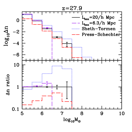
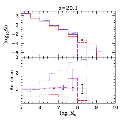
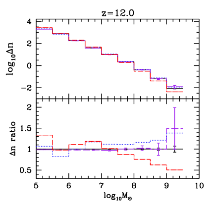
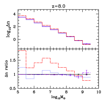
In Fig. 1 we show the mass functions in the mass range at selected redshifts based on the and simulations, together with PS and ST analytical mass functions. The actual quantities plotted are halo number densities , integrated over equal-size logarithmic mass bins. The last mass bin includes all haloes with mass . The two simulated mass functions show excellent agreement with each other, except for the high mass end, where the mass function is truncated due to finite volume. This agreement indicates the consistency of the N-body simulation over varying box size.
Compared to the analytical expressions, our N-body mass functions are in better agreement with ST than PS mass functions. The agreement with ST at all redshifts is within for , the haloes in which range numerically dominate the minihalo population. At very high redshifts, , ST mass function slightly over-predicts halo population at and under-predicts halo abundance at , with tendency to deviate increasingly as increases, while at relatively low redshifts, over-prediction occurs at . As discussed in Watson et al. (2014) these differences are partly due to our usage of a halo finder based on spherical overdensity instead of the friends-of-friends one used by ST, and also to the limitations of the ST fit which was based on low-redshift data and relatively small simulations. In contrast, the classical PS mass function gives a poor fit to N-body minihalo data at all redshifts, severely under-predicting the abundance of rare () haloes and over-predicting the abundance of haloes. Only for the most common () haloes PS is a more reasonable approximation (and also agrees with ST).
Assuming that the prescription for the conditional mass function (linking eq. 12 with unconditional mass function) provides a correct theoretical framework, one may expect that a good fit to unconditional mass function will also provide a good fit to conditional mass function when combined with eq. (12). Therefore, we can expect that will be the best fit to the mean conditional mass function from the simulations, and will also be a good fit, while will be a poor fit. We will test this expectation in Section 4.2.
4.2 Mean biased halo mass function
We now show how the mean, conditional mass functions of N-body haloes behave in terms of , and compare this to the modelling predictions based on the different mass functions, , and . We also compare these to the model based on the linear bias. The stochasticity in this relation will be treated in § 4.3.
4.2.1 Minihaloes
Minihaloes are usually defined by their hydrodynamical properties. Their minimum mass is the cosmic Jeans mass determined by the mean IGM temperature, and their maximum mass is the mass of haloes whose virial temperature is about . While this is the general definition, the uncertainty of the mean IGM temperature at high redshift makes the definition of the minimum mass somewhat uncertain. In this work we instead take their mass to be in a fixed range , which is of more direct use to N-body data at fixed mass resolution. Both and boxes resolve haloes down to . The latter simulation thus provides a better statistics by encompassing a volume 32 times as large as that of the former one.
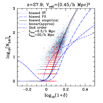
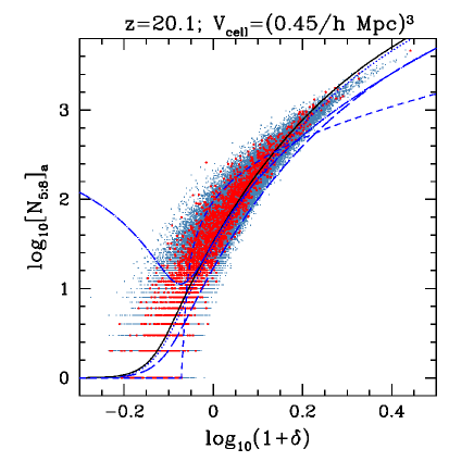
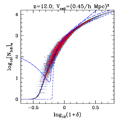
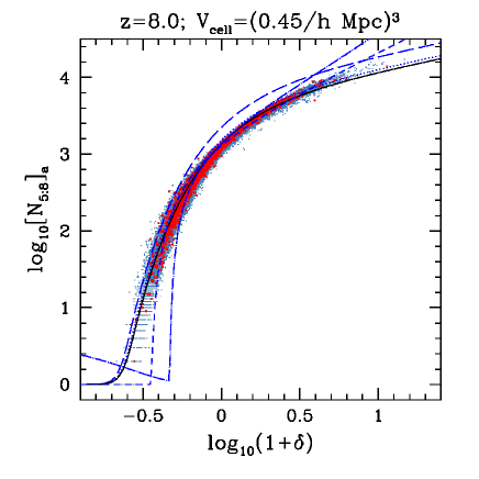
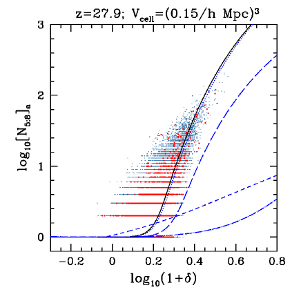
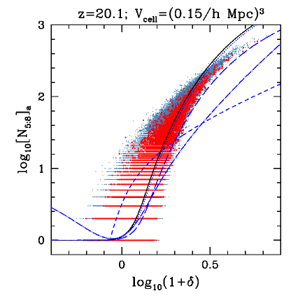
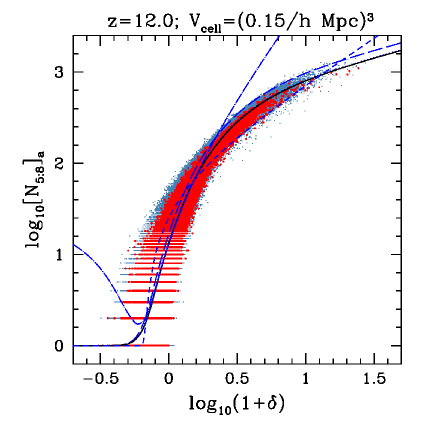
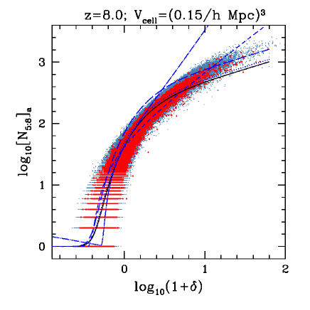
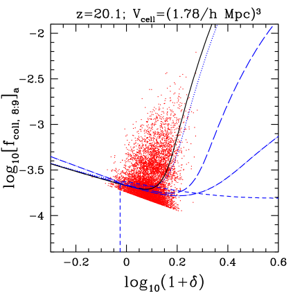
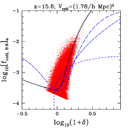
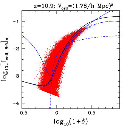
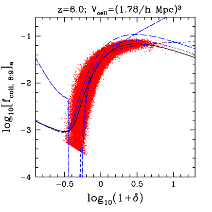
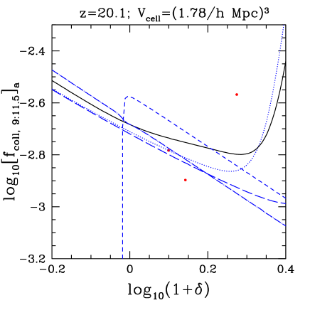
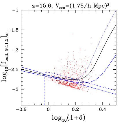
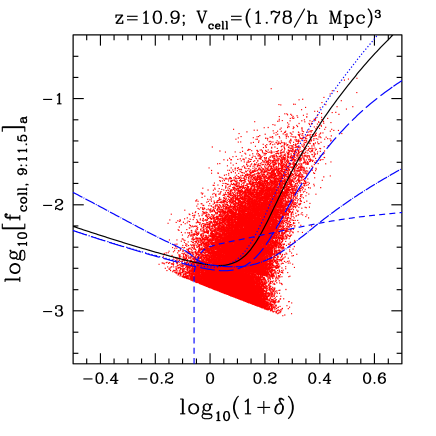
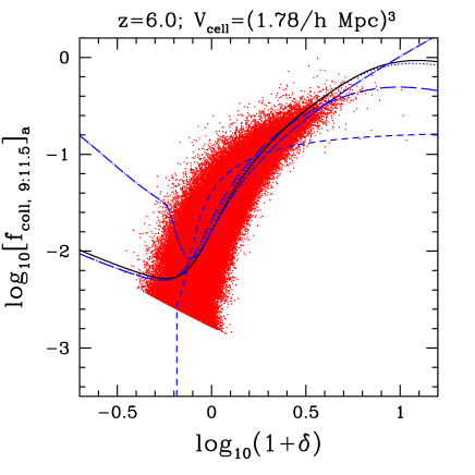
We first examine how well the models based on the analytical mass function fits match the N-body data. Figs 2 and 3 show the analytical estimates and N-body data on the total number of minihaloes under different Eulerian cell sizes. We find that the numerical data from the two simulation volumes is in excellent agreement and that and fit the N-body data well over almost the entire range of and , while and the linear relation both provide poor fits to the data in general. Even though and are integral quantities, given that smallest-mass haloes numerically dominate the halo population, both the data and semi-analytical estimates reflect predominantly the low-mass end. Note that as seen in Fig. 1, agrees well with in the low mass-end, and this is the reason why provides a good fit. If we focused on the high-mass end only, would be a very poor fit to the observed bias, because the average ST mass function has large discrepancy from the actual N-body data for e.g. . In contrast, the collapsed fraction in haloes (Figs 1 and 2 of the Supplementary Material) is a mass-weighted quantity and thus reflects the high mass end better than does , but the rapid exponential cutoff of the mean halo mass function at increasing still moderates the contribution from the high-mass haloes. The similarity between and reflect the simple fact that the unconditional mass functions, and , are similar around the low-mass end.
As the cell size shrinks, however, some discrepancy appears at high regime. Both and predictions overestimate the N-body data substantially at , when the volume of the cell has shrunken from to : see Fig. 3 At this point, where approaches the overdensity criterion for halo identification, we suspect that this could be a symptom of extreme nonlinearity: the mean mass of the cell, , is small enough to be comparable to the high-mass end of minihaloes, or .
In summary, unless the cell is too small, and thus potentially quite nonlinear, the mean nonlinear bias of N-body minihaloes at high redshifts can be explained well by the simple hybrid prescriptions and . In contrast, at high redshifts, the linear relation deviates too much from the N-body minihalo data to be of much practical use at least under the filtering scales of . The disagreement of with the N-body data is just as severe, and we expect that will be useless regardless of the filtering scale, because the disagreement is caused by the poorness of the mean PS mass function. It is notable that the rarity of haloes at high redshifts make the linear relation fail even when , which will be discussed in much detail in Section 4.4.
4.2.2 Atomically-cooling haloes
Atomically-cooling haloes (ACH hereafter) are named after the dominant cooling mechanism of baryonic gas inside. Atomic line radiation can cool primordial-composition gas to from its initially higher virial temperature. Star formation are believed to occur inside these haloes as pre-existing metals or newly-formed can further cool the gas down to . Therefore, ACHs are usually defined by their virial temperature: haloes with . As this threshold virial temperature roughly coincides with , here we define ACHs as those haloes with . The ACHs can be grouped further into low-mass ACHs (LMACH), for which the gas pressure of the photoheated IGM in an ionized patch prevented the halo from capturing the gas it needs to form stars, and high-mass ACHs (HMACH), for which gravity was strong enough to overcome this “Jeans-mass filter” and form stars even in the ionized patches. The dividing line between LMACHs and HMACHs occurred roughly at (although the precise boundary value is still uncertain).
As our box simulation resolves haloes of , ACHs defined as above are fully identified. Even though the inner structure of low-mass end haloes is not resolved near the resolution limit (see Section 2), for our considerations only the number count of haloes matters, both for the mean halo bias and stochasticity333As to be seen in § 3.4 and § 4.3, the conditional halo correlation function determines the stochasticity. The halo correlation function is composed of the 1-halo term and the 2-halo term, and the dominant contribution to stochasticity comes from the 2-halo term. Therefore, it is not required to fully resolve the halo structure in estimating the stochasticity. and therefore our results are not affected by this.
We choose two filtering scales, and . While these choices are somewhat arbitrary, we increased the filtering scales for ACHs from those for minihaloes, due to the increased rarity of ACHs. The halo collapsed fraction is plotted in Figs 4 and 5. While LMACHs have a finite range in mass, because HMACHs are defined to have a loose end, we assign their maximum mass as the one somewhat smaller than the mass of the average-density cell: and for cells with and , respectively. Otherwise, the bias formalism breaks down (equation 5). Overall, the mean values of both the LMACH collapsed fraction (), and the HMACH collapsed fraction ( and ) are well predicted by equation (16) when we adopt (equation 15). For LMACHs, provides as good a fit as , except at where ST prescription somewhat overestimates the mean. For HMACHs, the biggest discrepancy between and exist at higher redshifts (e.g. ) at : here the small number of sampled cells at high cell-density makes it difficult to conclude which prescription provides a better estimator for the mean bias. PS prescription provides a very poor fit at all redshifts.
The linear bias parameter, for both LMACHs and HMACHs, fails in predicting the mean bias in general. This is noteworthy because even in the linear regime, including the point , the linear bias parameter predicts the bias to be off from the observed values, which was also the case for minihaloes. We discuss this issue in detail in Section 4.4.
In summary, even though LMACHs and HMACHs are very rare in the regime we study, the nonlinear bias prescription combined with the mean N-body halo mass function fits the observed mean halo bias very well throughout the ranges of redshift and cell density we observe. Therefore, this hybrid bias prescription can be applied for astrophysical and cosmological applications in general. We have indeed applied the bias prescription from this work in simulating cosmic reionization by ACHs in a very large box, , in order to populate Eulerian cells with size (Iliev et al., 2014). Because the halo mass resolution of the corresponding N-body simulation was only , we assigned each cell the missing LMACHs using the mean conditional mass function , where the LMACH mean mass function from our simulation was used to generate .
4.3 Stochasticity
The average behaviour of conditional mass function is well understood in terms of the biased mass function . Now, how does the scatter of correlation around the mean compare to the expected stochasticity? We showed in Section 3.4 that the variance of the number of haloes and given deviate from the simple Poisson value by the amount . We now show the result of simulation and compare this to the Poisson statistics (equation 24) and (equation 19) by explicitly calculating the sub-cell-scale correlation function (equation 20).
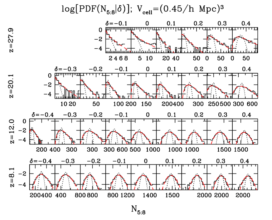
In Fig 6 (see also Figs 5–9 in Supplementary Material) we show the actual PDF and compare it to the expected Poisson distribution. We find that the empirical PDF does not follow pure Poisson distribution in general: the observed PDFs usually show large outliers compared to the Poisson distribution, and there is no convincing case with variance smaller than the Poissonian even though such a case is possible if haloes are anti-correlated under given density environment (equations 19–22). For example, Fig. 6 shows PDFs of minihalo population inside the Mpc box at different redshifts and ’s. In order to get the distribution, each chosen has some width such that cells are chosen if their overdensity lies inside . is taken to be narrow enough to guarantee that the PDF in each bin is a fair representation of the true PDF, while at the same time wide enough to generate a large number of cells for statistically reliable measure of the variance.
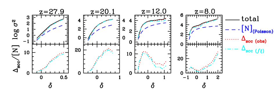
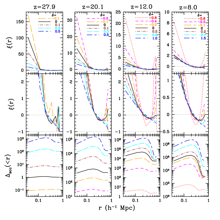
We also quantify the relative contribution of to by the ratio (note that it is compared not to but ), in order to see the degree of deviation of PDF from the pure Poisson distribution. There are several notable features in : (1) At a given redshift, the ratio decreases as mass of haloes increases, and thus LMACHs and HMACHs show much weaker outliers progressively. Fig. 6 and Figs 5–9 in Supplementary Material show this trend: MHs have , LMACHs have , and HMACHs have ; (2) As one increases the filtering scale – or the size of cells – tends to decrease overall. We nevertheless have some exceptions in this trend for MHs at very high-density cells (); (3) is not a monotonically increasing or decreasing function of ; and (4) is mostly positive both in underdense and overdense cells, indicating that the sub-cell correlation is overall positive in both regimes (see equation 20; this does not mean that there is no negative values in ). This contradicts the claim by Somerville et al. (2001), where they usually find that in underdense regions and in positive regions which led them to conclude that the correlation function is negative inside underdense regions and positive in overdense regions. We believe that this discrepancy comes from the erroneous definition of in Somerville et al. 2001, where they subtracted the global mean number of haloes averaged over all cells of such that , while one should indeed define this as in equation 22 to reflect the effect of the sub-cell correlation function. The observed anti-correlation of , or negative values of when becomes comparable to the cell size as seen in Fig. 7 (see also Figs 10–14 in Supplementary Material), is due to the finite cell size, because any correlation existing inside a cell should be counter-balanced by anti-correlation in order to conserve the halo number.
We explicitly calculate defined by equation (20) and from equation (19). Toward this, we place a uniform grid with sub-cells on each cell with , such that . We then sample all sub-cell pairs with given distance – discretized as the distance between centres of sub-cells – and calculate using equation (20) and using equation (19) We compare this value to the observed, residual variance , which are shown in the bottom panels of Fig. 6, denoted by and respectively. The agreement between the two quantities are excellent, and thus proves the fact that is the sole origin for the super-Poissonian (or sometimes sub-Poissonian) variance in (see also Figs 5–9 in Supplementary Material). Due to halo-number conservation, the correlation function is composed of positive (correlation) and negative (anti-correlation) parts as seen in Fig. 7 (and Figs 10–14 in Supplementary Material).
4.4 Bias in Perturbative Schemes
Local halo bias is often calculated or fitted in perturbative way, i.e. as a polynomial series of :
| (29) |
where the bias parameter is now defined as an th-order moment in this expansion. In practice, one should truncate the series by limiting such that higher order moments decay more rapidly than a few lowest-order moments. In this section, we re-visit the perturbative scheme by MW and examine in more detail.
Linear bias approximation, , is widely used in literature and in practical applications such as galaxy surveys for cosmology. Here, the linear bias parameter is useful when the mass of haloes is fixed, because then is a simple constant coefficient for varying , or , and the same relation applies to -space bias such that . Its limitation, however, has already been pointed out by MW themselves, by expanding the nonlinear relation (equation 12) to second order in and first order in . Such expansion (and truncation at some order) is useful in observing the halo bias in -space because algebraic connection between real-space parameters and -space parameters is possible, and also in understanding the generic behaviour of nonlinear bias. We therefore examine the Taylor-expanded form of equation (12). The main difference from MW is that we expand the nonlinear relation to second order in but keeping -dependence accurate, because we sometimes reach . This will enable us to examine the dependence of nonlinear bias on the filtering scale more accurately.
We thus Taylor-expand to the second order in while keeping the dependency on accurate (as in equation 30 of MW):
| (30) |
where we use as an expansion of (; see MW) and use the chain rule . Using equations (5) and (12), we obtain444Rigorously speaking, in this derivation, we assume that the filtering scale is fixed, and thus so is . Because , this means that the changes as , which is not compatible with the notion of uniform grid. If we were to apply the expanded form on uniform-grid cases instead, is fixed and thus and change as changes. Additional terms due to non-vanishing will appear on and in this case. Nevertheless, is a very slowly-varying function in at , and thus we expect it to be higher-order correction in , and simply assume that in the expansion in general.
| (31) |
| (32) |
and
| (33) |
where
| (34) |
and
| (35) |
MW approximate the dependence on to first order, and have , , and , to which equations (31), (32) and (33) converge respectively when .
explains the non-zero offsets and observed in almost all cases (see Figs 2-5): let us call this the “0-point offset” as MW did. 0-point offset is a natural consequence of the fact that the global mean of a quantity , , differs from the selective average, , only over cells with . If one is to apply a simple linear relation , it is presumed that (or ) because with as a constant coefficient. However, even in the linear regime in general, with non-zero . depends strongly on . The negative sign of reflects the fact that the rarer the haloes, or the higher the , the smaller the chances are to find them in the mean-density environment (); in the opposite regime when is small, , which means that haloes are more abundant in the mean-density cells than the mean value. The sign of also indicates, under a given filtering scale, the “overall” tendency of halo distribution: when , the net number of haloes found in overdense regions is larger than that in underdense regions, and when , the net number of haloes found in overdense regions is smaller than that in underdense regions. As a practical example, it will be very important to study haloes in voids if those haloes are a very abundant type, or .
It is important to note that if the bias function (equation 10) is expanded instead of , one should include the singular term such that , because otherwise the approximated linear bias parameter cannot explain the offset. In this sense, should not be taken as a physical quantity but merely as a mathematical entity representing the fully nonlinear dependence of on . () is a physical quantity which does not become singular when .
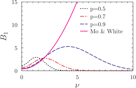
is a good indicator of the overall trend of bias. The sign of , which is always positive, guarantees that haloes are not anti-biased but biased for higher cell-densities regardless of or the filtering scale, as long as is in the linear regime. depends on both and . At fixed halo-mass and filtering scale, increases as increases when and decreases when (figure 8). Such non-monotonic trend in would not be observed when filtering scale is large enough, because then . At fixed halo mass (and thus fixed and at some ), the effect of filtering scale or on is also a mixed bag depending on rarity of haloes (or ) as seen in figure 8.
5 Summary and Discussion
We investigated the local bias of cosmological halo formation in the fully nonlinear regime, using both halo data from N-body simulations sampled on uniform grids and theoretical estimates for Eulerian halo bias. Over the wide dynamic range of halo mass, from to , we find that the observed biased population of haloes inside a cell with density can be matched well by the convolution of the mean N-body mass function with the nonlinear bias parameter derived from the extended Press-Schechter formalism. Convolution with the PS mass function provides very poor fits in general, and convolution with the ST mass function provides fits slightly poorer than . Nevertheless, as the ST mass function is known to break down for very rare haloes (see e.g. the large discrepancy of the ST mass function for haloes of at in Fig. 1), it is best to avoid both PS and ST, and instead use in convolving the mean mass function to the bias factor given by equation (12). Based on the fact that the observed bias in halo population is well matched by the hybrid estimate which combines two physical quantities with different origins (the average mass function is determined by a specific halo-identification scheme and the nonlinear bias parameter is based on the extended Press-Schechter theory), this prescription should be applicable in general to cases under other halo-identification schemes.
We also find that the variance of halo numbers inside grid cells with given overdensity is not purely Poissonian, but has additional variance. This variance originates from the sub-cell scale halo-halo correlation, which we proved quantitatively by explicitly calculating the conditional correlation functions. In the regime we studied ( and uni-grid filtering with cell size of ), we find that the additional variance is always positive except for some negative values sporadically observed for haloes with .
The nonlinear bias prescription described in our paper can be used to generate mock halo catalogues in the following sequence:
(i) Generate or adopt a mean mass function of haloes . It is advised not to use the PS mass function, due to the large discrepancy from the usual N-body halo catalogues practically over the full mass range.
(ii) Generate a density field at a redshift of interest: if N-body data is available, adopt a proper smoothing scheme to generate a density field from the distribution of particles. Depending on the size of cells, cell-density can become nonlinear, and therefore N-body simulation is recommended.
(iii) Place a uniform grid on the density field from step (ii), and identify the comoving volume of the cell as .
(iv) Visit a cell, and identify the cell overdensity . Use equation (4) to deduce . Take as the spatial filtering scale of the linearly extrapolated density field to , and calculate the corresponding variance . Use equations (7) and (8) (or the numerical fit given by equation 18 of MW) to find matching of .
(v) To populate a cell with a halo of mass , use equation (3) to obtain , and take this as the filtering scale of the lineaized density field at and calculate the corresponding variance .
(vi) Plug quantities from steps (iv) and (v) in equation (5), then use equation (6), then finally use equation (15) to calculate the biased halo mass function . Multiplying the infinitesimal mass bin and to , one obtains the mean number of haloes of in the cell.
(vii) Iterate steps (iv) - (vi) over all cells in the box.
(viii) If one wants to implement stochasticity, which should indeed affect the power spectrum of halo density field, use equation (23) with from step (vi) and an empirically found to include super-Poisson stochasticity and sample halos by the Monte-Carlo method. For a selected range of halo masses and cell sizes as described in Sections 4.2 and 4.3, a reader may contact us for these values.
Perturbative approach to the nonlinear bias is found limited. First, one needes to be careful when approximating the halo bias by a simple linear relation , because even when the filtered density field is in the linear regime, , the 0-point offset (equation 31) may not be negligible. In such cases, one should of course take into account such that . This 0-point offset () occurs in general when (1) haloes are rare and/or (2) the cell size is small, which MW has already recognized and we have confirmed from our data. In the nonlinear regime, even the second-order perturbation, which we calculated without the approximation taken by MW (Equations 31 – 35), provides a very poor fit in general. We thus claim that the local nonlinear bias scheme should be used unless perturbative approach is unavoidable.
Nonlinear bias schemes such as the one studied in this paper can be applied to both cosmological and astrophysical problems. For example, we already used the mean bias prescription in this paper as a sub-grid treatment to populate simulation boxes with haloes which are not resolved otherwise, for simulating cosmic reionization process: see Ahn et al. (2012) for populating box with minihaloes, and Iliev et al. (2014) for populating box with LMACHs. Similar approach has been attempted by de la Torre & Peacock (2013), where they test their bias-based sub-grid treatment against resolved N-body haloes in terms of two-point statistics. Their bias prescription, however, is heuristic and thus the corresponding fitting parameters should be re-evaluated when e.g. a very different dynamic range of halo mass is targeted. In contrast, even though we have just studied cosmological haloes at , the agreement between data and theoretical prediction in such wide range of halo mass, cell size, cell density, and redshift suggest that this prescription is valid in general.
The nonlinear bias scheme studied here is valid when the primordial density field is Gaussian, and thus may not be directly used to study non-Gaussianity. It is also preferred that further study of the super-Poissonian (or sometimes sub-Poissonian) stochasticity, which we quantified here with box for minihaloes and box for LMACHs and HMACHs, is devised with higher-resolution, larger-box simulations to increase statistical reliability. Stochasticity is likely to have temporal correlation as well as spatial correlation, which should be further studied for a more self-contained bias prescription.
Acknowledgments
This work was supported by a research grant from Chosun University (2010). All simulations in this work were undertaken at the Texas Advanced Computing Center (TACC) at The University of Texas at Austin under TeraGrid allocations.
References
- Adshead et al. (2012) Adshead P., Baxter E. J., Dodelson S., Lidz A., 2012, Phys. Rev. D , 86, 063526
- Ahn et al. (2012) Ahn K., Iliev I. T., Shapiro P. R., Mellema G., Koda J., Mao Y., 2012, ApJL, 756, L16
- Alvarez et al. (2009) Alvarez M. A., Busha M., Abel T., Wechsler R. H., 2009, ApJL, 703, L167
- Baldauf et al. (2013) Baldauf T., Seljak U., Smith R. E., Hamaus N., Desjacques V., 2013, Phys. Rev. D , 88, 083507
- Bardeen et al. (1986) Bardeen J. M., Bond J. R., Kaiser N., Szalay A. S., 1986, ApJ, 304, 15
- Barkana & Loeb (2004) Barkana R., Loeb A., 2004, ApJ, 609, 474
- Bond et al. (1991) Bond J. R., Cole S., Efstathiou G., Kaiser N., 1991, ApJ, 379, 440
- Ciardi & Ferrara (2005) Ciardi B., Ferrara A., 2005, Space Science Reviews, 116, 625
- Cole & Kaiser (1989) Cole S., Kaiser N., 1989, MNRAS, 237, 1127
- Dalal et al. (2008) Dalal N., Doré O., Huterer D., Shirokov A., 2008, Phys. Rev. D , 77, 123514
- D’Aloisio et al. (2013) D’Aloisio A., Zhang J., Jeong D., Shapiro P. R., 2013, MNRAS, 428, 2765
- Datta et al. (2012) Datta K. K., Friedrich M. M., Mellema G., Iliev I. T., Shapiro P. R., 2012, MNRAS, 424, 762
- de la Torre & Peacock (2013) de la Torre S., Peacock J. A., 2013, MNRAS, 435, 743
- Dekel & Lahav (1999) Dekel A., Lahav O., 1999, ApJ, 520, 24
- Friedrich et al. (2011) Friedrich M. M., Mellema G., Alvarez M. A., Shapiro P. R., Iliev I. T., 2011, MNRAS, 413, 1353
- Furlanetto & Oh (2005) Furlanetto S. R., Oh S. P., 2005, MNRAS, 363, 1031
- Furlanetto, Zaldarriaga & Hernquist (2004) Furlanetto S. R., Zaldarriaga M., Hernquist L., 2004, ApJ, 613, 1
- Harnois-Déraps et al. (2013) Harnois-Déraps J., Pen U.-L., Iliev I. T., Merz H., Emberson J. D., Desjacques V., 2013, MNRAS, 436, 540
- Iliev et al. (2014) Iliev I. T., Mellema G., Ahn K., Shapiro P. R., Mao Y., Pen U.-L., 2014, MNRAS, 439, 725
- Jenkins et al. (2001) Jenkins A., Frenk C. S., White S. D. M., Colberg J. M., Cole S., Evrard A. E., Couchman H. M. P., Yoshida N., 2001, MNRAS, 321, 372
- Joudaki et al. (2011) Joudaki S., Doré O., Ferramacho L., Kaplinghat M., Santos M. G., 2011, Phys. Rev. Lett., 107, 131304
- Kaiser (1984) Kaiser N., 1984, ApJL, 284, L9
- Kitaura, Yepes & Prada (2014) Kitaura F.-S., Yepes G., Prada F., 2014, MNRAS, 439, L21
- Lim & Lee (2013) Lim S., Lee J., 2013, J. Cosmol. Astropart. Phys. , 1, 19
- Lukić et al. (2007) Lukić Z., Heitmann K., Habib S., Bashinsky S., Ricker P. M., 2007, ApJ, 671, 1160
- Manera et al. (2013) Manera M. et al., 2013, MNRAS, 428, 1036
- Manera, Sheth & Scoccimarro (2010) Manera M., Sheth R. K., Scoccimarro R., 2010, MNRAS, 402, 589
- Mao et al. (2013) Mao Y., D’Aloisio A., Zhang J., Shapiro P. R., 2013, Phys. Rev. D , 88, 081303
- Mesinger, Furlanetto & Cen (2011) Mesinger A., Furlanetto S., Cen R., 2011, MNRAS, 411, 955
- Mo & White (1996) Mo H. J., White S. D. M., 1996, MNRAS, 282, 347
- Monaco et al. (2013) Monaco P., Sefusatti E., Borgani S., Crocce M., Fosalba P., Sheth R. K., Theuns T., 2013, MNRAS, 433, 2389
- Monaco et al. (2002) Monaco P., Theuns T., Taffoni G., Governato F., Quinn T., Stadel J., 2002, ApJ, 564, 8
- Neyrinck et al. (2014) Neyrinck M. C., Aragón-Calvo M. A., Jeong D., Wang X., 2014, MNRAS, 441, 646
- Park et al. (2013) Park H., Shapiro P. R., Komatsu E., Iliev I. T., Ahn K., Mellema G., 2013, ApJ, 769, 93
- Peebles (1993) Peebles P. J. E., 1993, Principles of physical cosmology. Princeton Series in Physics, Princeton, NJ: Princeton University Press, —c1993
- Press & Schechter (1974) Press W. H., Schechter P., 1974, ApJ, 187, 425
- Reed et al. (2007) Reed D. S., Bower R., Frenk C. S., Jenkins A., Theuns T., 2007, MNRAS, 374, 2
- Santos et al. (2008) Santos M. G., Amblard A., Pritchard J., Trac H., Cen R., Cooray A., 2008, ApJ, 689, 1
- Saslaw & Hamilton (1984) Saslaw W. C., Hamilton A. J. S., 1984, ApJ, 276, 13
- Scoccimarro & Sheth (2002) Scoccimarro R., Sheth R. K., 2002, MNRAS, 329, 629
- Shapiro et al. (2013) Shapiro P. R., Mao Y., Iliev I. T., Mellema G., Datta K. K., Ahn K., Koda J., 2013, Phys. Rev. Lett., 110, 151301
- Sheth (1995) Sheth R. K., 1995, MNRAS, 274, 213
- Sheth & Tormen (1999) Sheth R. K., Tormen G., 1999, MNRAS, 308, 119
- Sheth & Tormen (2002) Sheth R. K., Tormen G., 2002, MNRAS, 329, 61
- Somerville et al. (2001) Somerville R. S., Lemson G., Sigad Y., Dekel A., Kauffmann G., White S. D. M., 2001, MNRAS, 320, 289
- Warren et al. (2006) Warren M. S., Abazajian K., Holz D. E., Teodoro L., 2006, ApJ, 646, 881
- Watson et al. (2014) Watson W. A., Iliev I. T., Diego J. M., Gottlöber S., Knebe A., Martínez-González E., Yepes G., 2014, MNRAS, 437, 3776
- Zahn et al. (2007) Zahn O., Lidz A., McQuinn M., Dutta S., Hernquist L., Zaldarriaga M., Furlanetto S. R., 2007, ApJ, 654, 12