On the Spectral Efficiency of Full-Duplex Small Cell Wireless Systems

Abstract

We investigate the spectral efficiency of full-duplex small cell wireless systems, in which a full-duplex capable base station (BS) is designed to send/receive data to/from multiple half-duplex users on the same system resources. The major hurdle for designing such systems is due to the self-interference at the BS and co-channel interference among users. Hence, we consider a joint beamformer design to maximize the spectral efficiency subject to certain power constraints. The design problem is first formulated as a rank-constrained optimization one, and the rank relaxation method is then applied. However the relaxed problem is still nonconvex, and thus optimal solutions are hard to find. Herein, we propose two provably convergent algorithms to obtain suboptimal solutions. Based on the concept of the Frank-Wolfe algorithm, we approximate the design problem by a determinant maximization program in each iteration of the first algorithm. The second method is built upon the sequential parametric convex approximation method, which allows us to transform the relaxed problem into a semidefinite program in each iteration. Extensive numerical experiments under small cell setups illustrate that the full-duplex system with the proposed algorithms can achieve a large gain over the half-duplex one.

I Introduction

The ever growing demand of high data rates and proliferation of a number of users for wireless services have asked for modern communications technologies that exploit finite radio resources more efficiently. Among those, the multiple-input multiple-output (MIMO) communications technique [1] has gradually become a core component to many wireless communications standards such as LTE [2] and WiMAX [3]. In the physical layer of wireless communications networks, MIMO techniques are employed in both downlink and uplink transmissions. Due to practical limitations on hardware designs, downlink and uplink channels are currently designed to operate in one dimension (i.e., either in time or frequency domain). For example, cellular networks with time division duplex allocate the same frequency band, but different time slots, to downlink and uplink channels. On the other hand, cellular networks with frequency division duplex allow downlink and uplink transmissions to take place in the same time slot, but over distinct frequencies. Consequently, the radio resources have not been maximally used in existing wireless communications systems.

Full-duplex transmissions have recently gained significant attention owing to the potential to further improve or even double the capacity of conventional half-duplex systems. The benefits of full-duplex systems are of course brought by allowing the downlink and uplink channels to function at the same time and frequency [4, 5, 6, 7, 8, 9, 10, 11, 12, 13, 14, 15, 16, 17, 18, 19]. Though the gains of full-duplex systems can be easily foreseen, practical implementations of such full-duplex systems pose many challenges and a lot of technical problems still need to be solved before we can see the first trial deployment on a system level. The crucial barrier in implementing full-duplex systems resides in the self-interference (SI) from the transmit antennas to receive antennas at a wireless transceiver. More explicitly, the radiated power of the downlink channel interferes with its own desired received signals in the uplink channel. Clearly, the performance of full-duplex systems depends on the capability of self-interference cancellation at the transceiver which is limited in practice. In the past full-duplex transmission was thought infeasible. This is because the self-interference power, if not efficiently suppressed, significantly raises the noise floor at receive antennas, exceeding a limited dynamic range of the analog-to-digital converter (ADC) in the receiving device [7].

In recent years, many breakthroughs in hardware design for self-interference cancellation techniques have been reported, e.g., in [4, 6, 5, 17]. Especially, these studies demonstrate the feasibility of full-duplex transmission for short to medium range wireless communications. Since then, several studies focusing on full-duplex communications have been carried out in a variety of contexts such as point to point MIMO [13, 8, 11], MIMO relay [10, 18, 19], cognitive radio [12], and multiuser MIMO systems [9, 14]. With the aim of accelerating full-duplex applications in practical wireless systems, the full-duplex radios for local access (DUPLO) project has been funded by the European community’s seventh framework program [16]. As a first step, the first deliverable of the DUPLO project has identified several potential deployment scenarios that may benefit from full-duplex communications [15]. Among others, small cell wireless communications systems are selected as one of the important research frameworks. In fact, small cell systems are considered to be especially suitable for deployment of full-duplex technology due to low transmit powers, short transmission distances and low mobility.

What is missing in [15] is further studies that evaluate the actual gain of the full-duplex transmission for some reference systems. The goal of this paper is to fill this gap. Particularly, we consider a scenario where a full-duplex capable base station (BS) communicates with half-duplex users in both directions at the same time slot over the same frequency band. It is now well known that the optimal transmit strategy for downlink channels is achieved by dirty paper coding [20], but it requires high complexity to implement. Thus, we adopt a linear beamforming technique for the downlink transmission in this paper, which has been widely used in the literature, e.g., in [21, 22, 23]. For uplink channels, the optimal nonlinear multiuser detection scheme based on minimum mean square error and successive interference cancellation (MMSE-SIC) [24] is chosen in this paper. For the considered full-duplex system, the problem of beamformer design becomes more challenging since there still exists a small, but not negligible, amount of the self-interference between the transmit and receive antennas at the BS even after an advanced SI cancellation technique is applied. We note also that the SI level increases with the transmit power for any SI cancellation technique. Moreover, the difficulty of the design problem is increased further by the co-channel interference (CCI) caused by the users in the uplink channel to those in the downlink channel. By this very nature, a joint design of the downlink and uplink transmissions would offer the best solution. One of the first attempts to investigate the potential gain of full-duplex systems has been made in our earlier work of [9, 14]. However the CCI is not taken into account and several system parameters were ideally assumed therein. These practical considerations are carefully examined in this paper.

We are concerned with the problem of joint beamformer design to maximize the spectral efficiency (SE) under some power constraints. To this end, the total SE maximization (SEMax) problem is first formulated as a rank-constrained optimization problem for which it is difficult to find globally optimal solutions in general. The standard method of rank relaxation is then applied to arrive at a relaxed problem, which is still nonconvex. After solving the relaxed problem, the randomization technique presented in [25] is employed to find the beamformers for the original design problem. We note that the rank relaxation technique, commonly known as semidefinite relaxation (SDR) method under various contexts, is widely used to solve the problem of linear precoder design in MIMO downlink channels, e.g., in [25, 26, 27, 28, 29, 22]. Very often, the relaxed problems in those cases are convex and general convex program solvers can be called upon to find the solutions. Moreover, in some special cases, the rank relaxation is proved to be tight [21, 27, 29]. The same property unfortunately does not carry over into our case.

To tackle the nonconvexity of the relaxed problem, we propose two iterative local optimization algorithms. The first proposed algorithm is a direct result of exploiting the ‘difference of convex’ (D.C) structure of the relaxed problem. To be specific, based on the idea of the Frank-Wolfe (FW) algorithm [30], we arrive at a determinant maximization (MAXDET) program at each iteration. The second design approach involves some transformations before invoking the framework of sequential parametric convex approximation (SPCA) method [31], which has proven to be an effective tool for numerical solutions of nonconvex optimization problems [23, 32, 31]. In particular, we are able to approximate the relaxed problem as a semidefinite program (SDP) at each iteration in the second iterative algorithm. While the first design algorithm sticks to MAXDET problem solvers, the second one offers more flexibility in choosing optimization software and can take advantage of many state-of-the-art SDP solvers. Additionally, since there is no (even rough) way to estimate beforehand which algorithm is better than the other for a given set of channel realizations, the two iterative algorithms can be implemented in a concurrent manner and a solution is obtained when one of them terminates. Alternatively, we run the two algorithms in parallel until they converge, and then select the better solution. The numerical results on the SE and computational complexity of the two methods are given in Section IV.

Full-duplex transmission, if successfully implemented, is clearly expected to improve the spectral efficiency of wireless communications systems. However, a quantitative answer on the potential gains for some particular scenarios is still missing. For this purpose, the proposed algorithms are used to evaluate the performance of the full-duplex system of consideration under the 3GPP LTE specifications for a small cell system. The numerical experiments demonstrate that small cell full-duplex transmissions are superior to the conventional half-duplex one as long as the self-interference power is efficiently canceled.

The rest of the paper is organized as follows. The full-duplex system model and problem formulation are presented in Section II. In Section III, we describe the proposed iterative beamformer designs. The SE performance of the considered full-duplex transmission is numerically compared to the conventional half-duplex one in Section IV. Finally, the paper concludes with future work in Section V.

Notation: We use standard notations in this paper. Namely, bold lower and upper case letters represent vectors and matrices, respectively; $\mathbf{H}^{H}$ and $\mathbf{H}^{T}$ are Hermitian and standard transpose of $\mathbf{H}$, respectively; $\operatorname{Tr}(\mathbf{H})$ and $|\mathbf{H}|$ are the trace and determinant of $\mathbf{H}$, respectively; $\mathbf{H}\succeq\mathbf{0}$ means that $\mathbf{H}$ is a positive semidefinite matrix; $\operatorname{rank}(\mathbf{H})$ is rank of $\mathbf{H}$; $\nabla_{\mathbf{X}}\,f(\mathbf{X})$ is the gradient of $f(\mathbf{X})$; $E(\cdot)$ denotes the expectation operator.

II System Model and Problem Formulation

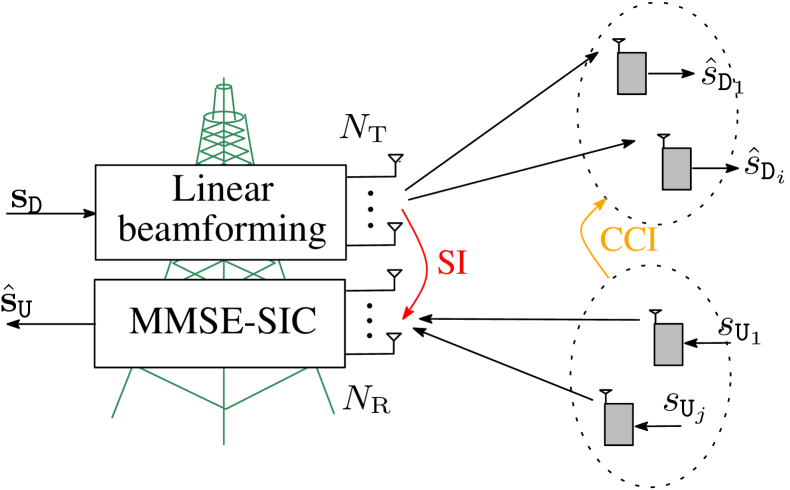
Figure 1: A small cell full-duplex wireless communications system. The number of transmit and receive antennas at the BS is $N_{\mathtt{T}}$ and $N_{\mathtt{R}}$, respectively. Linear beamforming is adopted for the downlink channel, while MMSE-SIC for the uplink channel. In the figure, SI and CCI mean self-interference and co-channel interference, respectively.

We consider a small cell full-duplex wireless communications system in which a full-duplex capable BS is designed to communicate with $K_{\mathtt{D}}$ single-antenna users in the downlink channel and $K_{\mathtt{U}}$ single-antenna users in the uplink channel at the same time over the same frequency band, as depicted in Fig. 1. Throughout the paper, the notations $\mathtt{D}_{i}$ and $\mathtt{U}_{j}$ refer to the $i$th and $j$th user in the downlink and uplink channels, respectively. The total number of antennas at the full-duplex BS is $N=N_{\mathtt{T}}+N_{\mathtt{R}}$, of which $N_{\mathtt{T}}$ transmit antennas are used for data transmissions in the downlink channel and $N_{\mathtt{R}}$ receive antennas are dedicated to receiving data in the uplink channel. We further assume that the channels are flat fading and channel state information (CSI) is perfectly known at both the BS and users.

First, in the downlink channel, let $s_{\mathtt{D}_{i}}$ be the transmitted data symbol for $\mathtt{D}_{i}$, which is normalized to $E(\bigl{|}s_{\mathtt{D}_{i}}\bigr{|}^{2})=1$. For linear beamforming, the data symbol $s_{\mathtt{D}_{i}}$ is multiplied by the beamforming vector $\mathbf{w}_{\mathtt{D}_{i}}\in\mathbb{C}^{N_{\mathtt{T}}\times 1}$ before transmission, and the received signal of user $\mathtt{D}_{i}$ is given by

$$y_{\mathtt{D}_{i}}=\mathbf{h}_{\mathtt{D}_{i}}^{H}\mathbf{w}_{\mathtt{D}_{i}}s_{\mathtt{D}_{i}}+\underbrace{\sum_{k\neq i}^{K_{\mathtt{D}}}\mathbf{h}_{\mathtt{D}_{i}}^{H}\mathbf{w}_{\mathtt{D}_{k}}s_{\mathtt{D}_{k}}}_{\textrm{MUI}}+\underbrace{\sum_{j=1}^{K_{\mathtt{U}}}g_{ji}s_{\mathtt{U}_{j}}}_{\textrm{CCI}}+n_{\mathtt{D}_{i}}$$ (1)

where $\mathbf{h}_{\mathtt{D}_{i}}$ is the $N_{\mathtt{T}}\times 1$ complex channel vector from the BS to user $\mathtt{D}_{i}$, $g_{ji}$ is the complex channel coefficient from $\mathtt{U}_{j}$ to $\mathtt{D}_{i}$, $s_{\mathtt{U}_{j}}$ is the data symbol transmitted by $\mathtt{U}_{j}$ in the uplink direction, and $n_{\mathtt{D}_{i}}\sim\mathcal{CN}(0,\sigma_{n}^{2})$ is background noise assumed to be additive white Gaussian (AWGN). In (1), the first and second summations represent multiuser interference (MUI) in the downlink channel and co-channel interference (CCI) from the uplink to the downlink channels, respectively. The received signal to interference plus noise ratio (SINR) of user $\mathtt{D}_{i}$ can be written as

$$\begin{array}[]{rl}\gamma_{\mathtt{D}_{i}}&=\dfrac{\bigl{|}\mathbf{h}_{\mathtt{D}_{i}}^{H}\mathbf{w}_{\mathtt{D}_{i}}\bigr{|}^{2}}{\sigma_{n}^{2}+\sum_{k\neq i}^{K_{\mathtt{D}}}\bigl{|}\mathbf{h}_{\mathtt{D}_{i}}^{H}\mathbf{w}_{\mathtt{D}_{k}}\bigr{|}^{2}+\sum_{j=1}^{K_{\mathtt{U}}}q_{\mathtt{U}_{j}}\bigl{|}g_{ji}\bigr{|}^{2}}\\ &=\dfrac{\mathbf{h}_{\mathtt{D}_{i}}^{H}\mathbf{Q}_{\mathtt{D}_{i}}\mathbf{h}_{\mathtt{D}_{i}}}{\sigma_{n}^{2}+\sum_{k\neq i}^{K_{\mathtt{D}}}\mathbf{h}_{\mathtt{D}_{i}}^{H}\mathbf{Q}_{\mathtt{D}_{k}}\mathbf{h}_{\mathtt{D}_{i}}+\sum_{j=1}^{K_{\mathtt{U}}}q_{\mathtt{U}_{j}}\bigl{|}g_{ji}\bigr{|}^{2}}\end{array}$$ (2)

where $E(|s_{\mathtt{U}_{j}}|^{2})=q_{\mathtt{U}_{j}}$, $j=1,...,K_{\mathtt{U}}$, is power loading for user $\mathtt{U}_{j}$ in the uplink direction; $\mathbf{Q}_{\mathtt{D}_{i}}=\mathbf{w}_{\mathtt{D}_{i}}\mathbf{w}_{\mathtt{D}_{i}}^{H}$, and $\operatorname{rank}(\mathbf{Q}_{\mathtt{D}_{i}})=1$. Then, spectral efficiency in the downlink direction is given by

$$R_{\mathtt{D}} = \sum_{i=1}^{K_{\mathtt{D}}}\log(1+\gamma_{\mathtt{D}_{i}})$$ (3a)

$$= \sum_{i=1}^{K_{\mathtt{D}}}\log\left(\frac{\sigma_{n}^{2}+\displaystyle\sum_{k=1}^{K_{\mathtt{D}}}\mathbf{h}_{\mathtt{D}_{i}}^{H}\mathbf{Q}_{\mathtt{D}_{k}}\mathbf{h}_{\mathtt{D}_{i}}+\sum_{j=1}^{K_{\mathtt{U}}}q_{\mathtt{U}_{j}}\bigl{|}g_{ji}\bigr{|}^{2}}{\sigma_{n}^{2}+\displaystyle\sum_{k\neq i}^{K_{\mathtt{D}}}\mathbf{h}_{\mathtt{D}_{i}}^{H}\mathbf{Q}_{\mathtt{D}_{k}}\mathbf{h}_{\mathtt{D}_{i}}+\sum_{j=1}^{K_{\mathtt{U}}}q_{\mathtt{U}_{j}}\bigl{|}g_{ji}\bigr{|}^{2}}\right).$$ (4a)

Next, for the uplink transmission, we can express the received signal vector at the full-duplex BS as

$$\mathbf{y}_{\mathtt{U}}=\sum_{j=1}^{K_{\mathtt{U}}}\mathbf{h}_{\mathtt{U}_{j}}s_{\mathtt{U}_{j}}+\underbrace{\sum_{i=1}^{K_{\mathtt{D}}}\mathbf{H}_{\mathtt{SI}}\mathbf{w}_{\mathtt{D}_{i}}s_{\mathtt{D}_{i}}}_{\textrm{self-interference}}+\mathbf{n}_{\mathtt{U}}$$ (5)

where $\mathbf{h}_{\mathtt{U}_{j}}\in\mathbb{C}^{N_{\mathtt{R}}\times 1}$ is the complex channel vector from the BS to $\mathtt{U}_{j}$ and $\mathbf{n}_{\mathtt{U}}\sim\mathcal{CN}(0,\sigma_{n}^{2}\mathbf{I}_{N_{\mathtt{R}}})$. The matrix $\mathbf{H}_{\mathtt{SI}}$ is called the self-interference channel from the transmit antennas to the receive antennas at the full-duplex BS, in which the values of its entries are determined by the capability of the advanced SI cancellation techniques. In this case, by treating the self-interference as background noise and applying the MMSE-SIC decoder, we can write the received SINR of $\mathtt{U}_{j}$ as [24]

$$\gamma_{\mathtt{U}_{j}}=q_{\mathtt{U}_{j}}\mathbf{h}_{\mathtt{U}_{j}}^{H}\Bigl{(}\sigma_{n}^{2}\mathbf{I}+\sum_{m>j}^{K_{\mathtt{U}}}q_{\mathtt{U}_{m}}\mathbf{h}_{\mathtt{U}_{m}}\mathbf{h}_{\mathtt{U}_{m}}^{H}+\sum_{i=1}^{K_{\mathtt{D}}}\mathbf{H}_{\mathtt{SI}}\mathbf{Q}_{\mathtt{D}_{i}}\mathbf{H}_{\mathtt{SI}}^{H}\Bigr{)}^{-1}\mathbf{h}_{\mathtt{U}_{j}}$$ (6)

where we have assumed a decoding order from $1$ to $K_{\mathtt{U}}$. Consequently, the achievable SE of the uplink channel is given by [24]

$$R_{\mathtt{U}} = \sum_{j=1}^{K_{\mathtt{U}}}\log(1+\gamma_{\mathtt{U}_{j}})$$ (8a)

$$= \sum_{j=1}^{K_{\mathtt{U}}}\log\Bigl{(}1+q_{\mathtt{U}_{j}}\mathbf{h}_{\mathtt{U}_{j}}^{H}\Bigl{(}\sigma_{n}^{2}\mathbf{I}+\sum_{m>j}^{K_{\mathtt{U}}}q_{\mathtt{U}_{m}}\mathbf{h}_{\mathtt{U}_{m}}\mathbf{h}_{\mathtt{U}_{m}}^{H}$$

$$+\sum_{i=1}^{K_{\mathtt{D}}}\mathbf{H}_{\mathtt{SI}}\mathbf{Q}_{\mathtt{D}_{i}}\mathbf{H}_{\mathtt{SI}}^{H}\Bigr{)}^{-1}\mathbf{h}_{\mathtt{U}_{j}}\Bigr{)}$$

$$= \log\dfrac{\Bigl{|}\sigma_{n}^{2}\mathbf{I}+{\displaystyle\sum_{i=1}^{K_{\mathtt{D}}}}\mathbf{H}_{\mathtt{SI}}\mathbf{Q}_{\mathtt{D}_{i}}\mathbf{H}_{\mathtt{SI}}^{H}+{\displaystyle\sum_{j=1}^{K_{\mathtt{U}}}}q_{\mathtt{U}_{j}}\mathbf{h}_{\mathtt{U}_{j}}\mathbf{h}_{\mathtt{U}_{j}}^{H}\Bigr{|}}{\Bigl{|}\sigma_{n}^{2}\mathbf{I}+{\displaystyle\sum_{i=1}^{K_{\mathtt{D}}}}\mathbf{H}_{\mathtt{SI}}\mathbf{Q}_{\mathtt{D}_{i}}\mathbf{H}_{\mathtt{SI}}^{H}\Bigr{|}}.$$ (9a)

From (1) and (5), we observe that the downlink and uplink transmissions are coupled by the CCI and self-interference. This problem greatly impacts the performance of the system of interest. Herein, our main purpose is to jointly design beamformers so that the total system spectral efficiency is maximized under the sum transmit power constraint in the downlink channel and per-user power constraints in the uplink one. Specifically, the total SEMax problem is formulated as a rank-constrained optimization one as

$$\underset{\{\mathbf{Q}_{\mathtt{D}_{i}}\},\{q_{\mathtt{U}_{j}}\}}{\operatorname{maximize}} R_{\mathtt{D}}+R_{\mathtt{U}}$$ (10a)

$$\operatorname{subject\;to} 0\leq q_{\mathtt{U}_{j}}\leq\overline{q}_{\mathtt{U}_{j}},\forall j=1,\ldots,K_{\mathtt{U}},$$ (10e)

$$\sum_{i=1}^{K_{\mathtt{D}}}\operatorname{Tr}(\mathbf{Q}_{\mathtt{D}_{i}})\leq P_{\mathtt{BS}},$$

$$\mathbf{Q}_{\mathtt{D}_{i}}\succeq 0,\forall i=1,\ldots,K_{\mathtt{D}},$$

$$\operatorname{rank}(\mathbf{Q}_{\mathtt{D}_{i}})=1,\forall i=1,\ldots,K_{\mathtt{D}}$$

where $P_{\mathtt{BS}}$ is the maximum power at the BS and $\overline{q}_{\mathtt{U}_{j}}$ is the power constraint at each user in the uplink channel. Clearly, problem (10) is a nonconvex program, which is difficult to solve optimally in general. We also note that a simplified problem of (10), in which $q_{\mathtt{U}_{j}}$ and $R_{\mathtt{U}}$ are omitted (i.e., the SEMax problem for the downlink channel itself), was proved to be NP-hard [33]. Thus, we conjecture that the NP-hardness is carried over into our problem. Towards a tractable solution, we first apply the relaxation method to obtain a relaxed problem of (10) by dropping the rank-1 constraints (10e). Then, two efficient iterative algorithms proposed to solve the resulting problem are presented in the next section.

III Proposed Beamformer Designs

Note that the relaxed problem of (10) after dropping the rank constraints is still nonconvex. Thus, computing its globally optimal solution is difficult and very computationally expensive in general. To the best of our knowledge, finding an optimal solution to the nonconvex problems similar to (10) is still an open problem. In this section, we present two reformulations of the relaxed problem, based on which two iterative algorithms of different level of complexity are developed.

III-A Iterative MAXDET-based Algorithm

The first beamforming algorithm is built upon an observation that the SE of the system at hand is a difference of two concave functions. Indeed, from (4a) and (9a), we can write $R_{\mathtt{D}}+R_{\mathtt{U}}=h(\mathbf{Q},\mathbf{q})-g(\mathbf{Q},\mathbf{q})$, where

$$h(\mathbf{Q},\mathbf{q})\triangleq\log\Bigl{|}\sigma_{n}^{2}\mathbf{I}+\sum_{i=1}^{K_{\mathtt{D}}}\mathbf{H}_{\mathtt{SI}}\mathbf{Q}_{\mathtt{D}_{i}}\mathbf{H}_{\mathtt{SI}}^{H}+\sum_{j=1}^{K_{\mathtt{U}}}q_{\mathtt{U}_{j}}\mathbf{h}_{\mathtt{U}_{j}}\mathbf{h}_{\mathtt{U}_{j}}^{H}\Bigr{|}\\ +\sum_{i=1}^{K_{\mathtt{D}}}\log\Bigl{(}\sigma_{n}^{2}+\sum_{k=1}^{K_{\mathtt{D}}}\mathbf{h}_{\mathtt{D}_{i}}^{H}\mathbf{Q}_{\mathtt{D}_{k}}\mathbf{h}_{\mathtt{D}_{i}}+\sum_{j=1}^{K_{\mathtt{U}}}q_{\mathtt{U}_{j}}|g_{ji}|^{2}\Bigr{)},$$ (11)

$$g(\mathbf{Q},\mathbf{q}) \triangleq \sum_{i=1}^{K_{\mathtt{D}}}\log\Bigl{(}\sigma_{n}^{2}+\sum_{k\neq i}^{K_{\mathtt{D}}}\mathbf{h}_{\mathtt{D}_{i}}^{H}\mathbf{Q}_{\mathtt{D}_{k}}\mathbf{h}_{\mathtt{D}_{i}}+\sum_{j=1}^{K_{\mathtt{U}}}q_{\mathtt{U}_{j}}|g_{ji}|^{2}\Bigr{)}$$ (12)

$$+\log\Bigl{|}\sigma_{n}^{2}\mathbf{I}+\sum_{i=1}^{K_{\mathtt{D}}}\mathbf{H}_{\mathtt{SI}}\mathbf{Q}_{\mathtt{D}_{i}}\mathbf{H}_{\mathtt{SI}}^{H}\Bigr{|}$$

and $\mathbf{Q}$ and $\mathbf{q}$ are the symbolic notations that denote the set of design variables $\{\mathbf{Q}_{\mathtt{D}_{i}}\}$ and $\{q_{\mathtt{U}_{j}}\}$, respectively. It should be noted that the functions $h(\mathbf{Q},\mathbf{q})$ and $g(\mathbf{Q},\mathbf{q})$ are jointly concave with respect to $\mathbf{Q}$ and $\mathbf{q}$ [34]. Borrowing the concept of the FW method which considers a linear approximation of the objective function and searches for a direction that improves the objective, we now present the first joint design algorithm to find $\mathbf{Q}$ and $\mathbf{q}$. First, the relaxed problem is reformulated as

$$\begin{array}[]{rl}\underset{{\scriptstyle\mathbf{Q},\mathbf{q}}}{\operatorname{maximize}}&{\displaystyle h(\mathbf{Q},\mathbf{q})-g(\mathbf{Q},\mathbf{q})}\\ \operatorname{subject\;to}&\eqref{eq:SE:c1},\;\eqref{eq:SE:c2},\;\eqref{eq:SE:c3}.\end{array}$$ (13)

Since the constraints (10e)-(10e) are convex, the difficulty in solving (13) lies in the component $-g(\mathbf{Q},\mathbf{q})$. Suppose the value of $(\mathbf{Q},\mathbf{q})$ at iteration $n$ is denoted by $(\mathbf{Q}^{(n)},\mathbf{q}^{(n)})$. To increase the objective in the next iteration we replace $g(\mathbf{Q},\mathbf{q})$ by its affine majorization at a neighborhood of $(\mathbf{Q}^{(n)},\mathbf{q}^{(n)})$. Since $g(\mathbf{Q},\mathbf{q})$ is concave and differentiable on the considered domain $\{\mathbf{Q}_{\mathtt{D}_{i}},q_{\mathtt{U}_{j}}:\mathbf{Q}_{\mathtt{D}_{i}}\succeq 0,q_{\mathtt{U}_{j}}\geq 0\}$, one can easily find an affine majorization as a first order approximation as [34]

$$g^{(n)}(\mathbf{Q},\mathbf{q})=g(\mathbf{Q}^{(n)},\mathbf{q}^{(n)})+\sum_{i=1}^{K_{\mathtt{D}}}\sum_{k=1,k\neq i}^{K_{\mathtt{D}}}\Bigl{[}\bigl{(}\vartheta_{\mathtt{D}_{i}}^{(n)}\bigr{)}^{-1}\mathbf{h}_{\mathtt{D}_{i}}^{H}\\ \bigl{(}\mathbf{Q}_{\mathtt{D}_{k}}-\mathbf{Q}_{\mathtt{D}_{k}}^{(n)}\bigr{)}\mathbf{h}_{\mathtt{D}_{i}}\Bigr{]}+\sum_{i=1}^{K_{\mathtt{D}}}\sum_{j=1}^{K_{\mathtt{U}}}\bigl{(}\vartheta_{\mathtt{D}_{i}}^{(n)}\bigr{)}^{-1}|g_{ji}|^{2}\bigl{(}q_{\mathtt{U}_{j}}-q_{\mathtt{U}_{j}}^{(n)}\bigr{)}\\ +\sum_{i=1}^{K_{\mathtt{D}}}\operatorname{Tr}\Bigl{[}\mathbf{H}_{\mathtt{SI}}^{H}\bigl{(}\boldsymbol{\Theta}^{(n)}\bigr{)}^{-1}\mathbf{H}_{\mathtt{SI}}\bigl{(}\mathbf{Q}_{\mathtt{D}_{i}}-\mathbf{Q}_{\mathtt{D}_{i}}^{(n)}\bigr{)}\Bigr{]}$$ (14)

where $\vartheta_{\mathtt{D}_{i}}^{(n)}$ and $\boldsymbol{\Theta}^{(n)}$ are defined as

$$\vartheta_{\mathtt{D}_{i}}^{(n)} = \sigma_{n}^{2}+\sum_{m\neq i}^{K_{\mathtt{D}}}\mathbf{h}_{\mathtt{D}_{i}}^{H}\mathbf{Q}_{\mathtt{D}_{m}}^{(n)}\mathbf{h}_{\mathtt{D}_{i}}+\sum_{l=1}^{K_{\mathtt{U}}}q_{\mathtt{U}_{l}}^{(n)}|g_{li}|^{2},$$ (15)

$$\boldsymbol{\Theta}^{(n)} = \sigma_{n}^{2}\mathbf{I}+\sum_{j=1}^{K_{\mathtt{D}}}\mathbf{H}_{\mathtt{SI}}\mathbf{Q}_{\mathtt{D}_{j}}^{(n)}\mathbf{H}_{\mathtt{SI}}^{H}.$$ (16)

To derive (14), we have used the fact $\nabla_{\mathbf{X}}\,\log|\mathbf{I}+\mathbf{A}\mathbf{X}\mathbf{A}^{H}|=\mathbf{A}^{H}(\mathbf{I}+\mathbf{A}\mathbf{X}\mathbf{A}^{H})^{-1}\mathbf{A}$, $\nabla_{x}\,\log(1+ax)=a(1+ax)^{-1}$, the inner product of two semidefinite matrices $\mathbf{X}\succeq\mathbf{0}$ and $\mathbf{Y}\succeq\mathbf{0}$ is $\operatorname{Tr}(\mathbf{XY})$, and the inner product of two vector is $\mathbf{x}^{H}\mathbf{y}$ [35]. Now, we approximate problem (13) at iteration $n+1$ by a convex program given by

$$\begin{array}[]{rl}\underset{{\scriptstyle\mathbf{Q},\mathbf{q}}}{\operatorname{maximize}}&h(\mathbf{Q},\mathbf{q})-g^{(n)}(\mathbf{Q},\mathbf{q})\\ \operatorname{subject\;to}&\eqref{eq:SE:c1},\;\eqref{eq:SE:c2},\;\eqref{eq:SE:c3}.\end{array}$$ (17)

The objective in (17) is in fact a lower bound of the SE of the full-duplex system. We note that problem (17) is a MAXDET program, and hence the name of the first algorithm. Let $(\mathbf{Q}^{\star},\mathbf{q}^{\star})$ be the optimal value of $(\mathbf{Q},\mathbf{q})$ in (17). Then we update $(\mathbf{Q}^{(n+1)},\mathbf{q}^{(n+1)}):=(\mathbf{Q}^{\star},\mathbf{q}^{\star})$. In this way, the design variables are iteratively updated and the lower bound of the SE increases after every iteration. Since the SE is bounded above due to the power constraints (10e) and (10e), the iterative procedure is guaranteed to converge. The iterative MAXDET-based algorithm is outlined in Algorithm 1. The convergence properties of Algorithm 1 are stated in Theorem 1.

Algorithm 1 Iterative MAXDET-based algorithm.

0:  

1:  Generate initial values for $\mathbf{Q}_{\mathtt{D}_{i}}^{(0)}$ for $i=1,2,\ldots,K_{\mathtt{D}}$ and $q_{\mathtt{U}_{j}}^{(0)}$ for $i=1,2,\ldots,K_{\mathtt{U}}$.

2:  Set $n:=0$.

2:  

3:  repeat

4:     Solve (17) and denote the optimal solutions as $(\mathbf{Q}^{\star},\mathbf{q}^{\star})$.

5:     Update: $\mathbf{Q}_{\mathtt{D}_{i}}^{(n+1)}:=\mathbf{Q}_{\mathtt{D}_{i}}^{\star}$; and $q_{\mathtt{U}_{j}}^{(n+1)}:=q_{\mathtt{U}_{j}}^{\star}$ .

6:     Set $n:=n+1$.

7:  until Convergence.

7:  

8:  Perform randomization to extract a rank-1 solution if required.

An important point to note here is that the iterative procedure in Algorithm 1 possibly returns a locally optimal solution to a relaxed problem of (10) at convergence. Obviously, if $\operatorname{rank}(\mathbf{Q}_{\mathtt{D}_{i}}^{\star})=1$, then $\mathbf{Q}_{\mathtt{D}_{i}}^{\star}$ is also feasible to (10) and the beamformer for $\mathtt{D}_{i}$ can be immediately recovered from the eigenvalue decomposition of $\mathbf{Q}_{\mathtt{D}_{i}}^{\star}$ [34] . However, this may not be the case since the rank-1 constraints are dropped. Thus, a method to extract the beamformer is required if a high-rank solution is obtained. For this purpose, we adopt the randomization technique presented in [25] which is mentioned in line 8 of Algorithm 1 and briefly described as follows. We first generate a random (column) vector $\mathbf{v}_{\mathtt{D}_{i}}$ whose elements are independently and uniformly distributed on the unit circle in the complex plane, and then calculate the eigen-decomposition of $\mathbf{Q}_{\mathtt{D}_{i}}^{\star}$ as $\mathbf{Q}_{\mathtt{D}_{i}}^{\star}=\mathbf{U}_{\mathtt{D}_{i}}\mathbf{\Sigma}_{\mathtt{D}_{i}}\mathbf{U}_{\mathtt{D}_{i}}^{H}$. Next a beamformer is taken as $\mathbf{\tilde{w}}_{\mathtt{D}_{i}}=\mathbf{U}_{\mathtt{D}_{i}}\mathbf{\Sigma}_{\mathtt{D}_{i}}^{\nicefrac{{1}}{{2}}}\mathbf{v}_{\mathtt{D}_{i}}$, which is feasible to the original design problem since $||\mathbf{\tilde{w}}_{\mathtt{D}_{i}}||_{2}^{2}=\operatorname{Tr}(\mathbf{U}_{\mathtt{D}_{i}}\mathbf{\Sigma}_{\mathtt{D}_{i}}^{\nicefrac{{1}}{{2}}}\mathbf{v}_{\mathtt{D}_{i}}\mathbf{v}_{\mathtt{D}_{i}}^{H}\mathbf{\Sigma}_{\mathtt{D}_{i}}^{\nicefrac{{1}}{{2}}}\mathbf{U}_{\mathtt{D}_{i}}^{H})=\operatorname{Tr}(\mathbf{Q}_{\mathtt{D}_{i}}^{\star})$ [25]. The obtained beamformer $\mathbf{\tilde{w}}_{\mathtt{D}_{i}}$ is then used to compute the resulting sum rate. We repeat this process for a number of randomization samples and pick up the one that offers the best sum rate. Our numerical results have shown that the high-rank solutions of $\{\mathbf{Q}_{\mathtt{D}_{i}}\}$ only occur when $\sigma_{\mathtt{SI}}^{2}$ is sufficiently large, which is not of practical importance since this is not the interesting case for the full-duplex systems. When $\operatorname{rank}(\mathbf{Q}_{\mathtt{D}_{i}})>1$, we also obverse that the largest eigenvalue significantly dominates the remaining ones. More explicitly, the largest eigenvalue is always $10$ times larger then the second largest one, meaning that $\mathbf{Q}_{\mathtt{D}_{i}}$ is not far from a rank-1 matrix. This explains the fact that the beamforming vectors returned by the randomization method offer a performance very close to that of the relaxed problem. Explicitly, the extracted solutions achieve a spectral efficiency performance always higher than $95\%$ of the upper bound given by the relaxed problem.

Although the objective in (17) is not a linear function with respect to the design parameters as in the original work of [30], (17) can be equivalently transformed into the problem of maximizing an affine function over a convex set as $\underset{\omega,\mathbf{Q},\mathbf{q}}{\max}\{\omega-g^{(n)}(\mathbf{Q},\mathbf{q})|h(\mathbf{Q},\mathbf{q})\geq\omega,\eqref{eq:SE:c1},\eqref{eq:SE:c2},\eqref{eq:SE:c3}\}$. Thus, Algorithm 1 can be considered as a variant of the FW method. It has been reported in many studies that the type of FW methods can efficiently exploit the hidden convexity of the problem [36, 37, 32]. Thus, the same results as the FW-type method can also be expected in the first proposed design algorithm. However, solvers for MAXDET programs are quite limited, compared to their counterparts for SDPs. Because none of the general convex program solvers are perfect for all problems, a more flexible choice of a problem solver is of practical importance.

III-B Iterative SDP-based algorithm

Motivated by the discussion above, we propose in this subsection an iterative SDP-based algorithm to solve the relaxed problem of (10). Specifically, based on the general framework of the SPCA method and proper transformations, we can iteratively approximate the relaxed problem of (10) by an SDP in each iteration. The second approach allows us to take advantage of a wide class of SDP solvers which are more and more efficient due to continuing progress in semidefinite programming. To begin with, due to the monotonicity of the $\log$ function, we first reformulate the relaxed problem of (10) as

$$\begin{array}[]{rl}\underset{\{\mathbf{Q}_{\mathtt{D}_{i}}\},\{q_{\mathtt{U}_{j}}\}}{\operatorname{maximize}}&\prod_{i=1}^{K_{\mathtt{D}}}(1+\gamma_{\mathtt{D}_{i}})\prod_{j=1}^{K_{\mathtt{U}}}(1+\gamma_{\mathtt{U}_{j}})\\ \operatorname{subject\;to}&\eqref{eq:SE:c1},\;\eqref{eq:SE:c2},\;\eqref{eq:SE:c3}\end{array}$$ (18)

which then can be rewritten as

$$\underset{{\scriptstyle\{\mathbf{Q}_{\mathtt{D}_{i}}\},\{q_{\mathtt{U}_{j}}\},\{t_{\mathtt{D}_{i}}\},\{t_{\mathtt{U}_{j}}\}}}{\operatorname{maximize}} \quad\prod_{i=1}^{K_{\mathtt{D}}}t_{\mathtt{D}_{i}}\prod_{j=1}^{K_{\mathtt{U}}}t_{\mathtt{U}_{j}}$$ (19a)

$$\operatorname{subject\;to} \quad 1+\gamma_{\mathtt{D}_{i}}\geq t_{\mathtt{D}_{i}},\;i=1,\ldots,K_{\mathtt{D}},$$ (20a)

$$\quad 1+\gamma_{\mathtt{U}_{j}}\geq t_{\mathtt{U}_{j}},\;j=1,\ldots,K_{\mathtt{U}},$$ (21a)

$$\quad t_{\mathtt{D}_{i}}\geq 1,\forall i;t_{\mathtt{U}_{j}}\geq 1,\forall j,$$ (22a)

$$\quad\eqref{eq:SE:c1},\;\eqref{eq:SE:c2},\;\eqref{eq:SE:c3}$$ (23a)

by using the epigraph form of (18) [34]. Note that maximizing a product of variables admits an SOC representation [23, 40]. Thus, we only need to deal with the nonconvex constraints in (20a) and (21a). Let us treat the constraint (20a) first. It is without loss of optimality to replace (20a) by following two constraints

$$\sigma_{n}^{2}+\sum_{k=1}^{K_{\mathtt{D}}}\mathbf{h}_{\mathtt{D}_{i}}^{H}\mathbf{Q}_{\mathtt{D}_{k}}\mathbf{h}_{\mathtt{D}_{i}}+\sum_{j=1}^{K_{\mathtt{U}}}q_{\mathtt{U}_{j}}|g_{ji}|^{2} \geq t_{\mathtt{D}_{i}}\beta_{\mathtt{D}_{i}},$$ (24a)

$$\sigma_{n}^{2}+\sum_{k\neq i}^{K_{\mathtt{D}}}\mathbf{h}_{\mathtt{D}_{i}}^{H}\mathbf{Q}_{\mathtt{D}_{k}}\mathbf{h}_{\mathtt{D}_{i}}+\sum_{j=1}^{K_{\mathtt{U}}}q_{\mathtt{U}_{j}}|g_{ji}|^{2} \leq \beta_{\mathtt{D}_{i}}$$ (24b)

where $\beta_{\mathtt{D}_{i}}$ is newly introduced variable and can be considered as the soft interference threshold of $\mathtt{D}_{i}$. The equivalence between (20a) and the two inequalities in (24a) and (24b) follows the same arguments as in [23] which can be justified as follows. At optimum, suppose the constraint in (24b) holds with inequality, i.e., $\sigma_{n}^{2}+\sum_{k\neq i}^{K_{\mathtt{D}}}\mathbf{h}_{\mathtt{D}_{i}}^{H}\mathbf{Q}_{\mathtt{D}_{k}}\mathbf{h}_{\mathtt{D}_{i}}+\sum_{j=1}^{K_{\mathtt{U}}}q_{\mathtt{U}_{j}}|g_{ji}|^{2}<\beta_{\mathtt{D}_{i}}$. Then, we form a new pair $(\bar{\beta}_{\mathtt{D}_{i}},\bar{t}_{\mathtt{D}_{i}})$ as $\bar{\beta}_{\mathtt{D}_{i}}\triangleq\beta_{\mathtt{D}_{i}}/c$ and $\bar{t}_{\mathtt{D}_{i}}\triangleq ct_{\mathtt{D}_{i}}$ where $c$ is a positive constant. Obviously, there exists a given $c>1$ such that (24b) is still met when $\beta_{\mathtt{D}_{i}}$ is replaced by $\bar{\beta}_{\mathtt{D}_{i}}$. Since $\bar{\beta}_{\mathtt{D}_{i}}\bar{t}_{\mathtt{D}_{i}}=\beta_{\mathtt{D}_{i}}t_{\mathtt{D}_{i}}$, i.e., the right side of (24a) remains the same, the constraint in (24a) is still satisfied. However, since $\bar{t}_{\mathtt{D}_{i}}>t_{\mathtt{D}_{i}}$ with $c>1$, a strictly higher objective of the design problem is obtained. This contradicts with assumption that we already obtained the optimal objective. Likewise, we can decompose (21a) into

$$x_{\mathtt{U}_{j}}^{2}\mathbf{h}_{\mathtt{U}_{j}}^{H}\mathbf{X}_{\mathtt{U}_{j}}^{-1}\mathbf{h}_{\mathtt{U}_{j}} \geq t_{\mathtt{U}_{j}}-1,$$ (25a)

$$q_{\mathtt{U}_{j}} \geq x_{\mathtt{U}_{j}}^{2}$$ (25b)

where $\mathbf{X}_{\mathtt{U}_{j}}\triangleq\sigma_{n}^{2}\mathbf{I}+\sum_{m>j}^{K_{\mathtt{U}}}q_{\mathtt{U}_{m}}\mathbf{h}_{\mathtt{U}_{m}}\mathbf{h}_{\mathtt{U}_{m}}^{H}+\sum_{i=1}^{K_{\mathtt{D}}}\mathbf{H}_{\mathtt{SI}}\mathbf{Q}_{\mathtt{D}_{i}}\mathbf{H}_{\mathtt{SI}}^{H}$ and $x_{\mathtt{U}_{j}}$ is an auxiliary variable. The purpose of introducing slack variable $x_{\mathtt{U}_{j}}$ will be clear shortly when we show that it is necessary to arrive at an SDP formulation. Now, we can equivalently transform (19a) into a more tractable form as

$$\underset{\underset{\mathbf{\beta}_{\mathtt{D}},\mathbf{x}_{\mathtt{U}}}{{\scriptstyle\mathbf{Q},\mathbf{q},\mathbf{t}_{\mathtt{D}},\mathbf{t}_{\mathtt{U}},}}}{\operatorname{maximize}} \quad\prod_{i=1}^{K_{\mathtt{D}}}t_{\mathtt{D}_{i}}\prod_{j=1}^{K_{\mathtt{U}}}t_{\mathtt{U}_{j}}$$ (26a)

$$\operatorname{subject\;to} \quad\sigma_{n}^{2}+\sum_{k=1}^{K_{\mathtt{D}}}\mathbf{h}_{\mathtt{D}_{i}}^{H}\mathbf{Q}_{\mathtt{D}_{k}}\mathbf{h}_{\mathtt{D}_{i}}+\sum_{j=1}^{K_{\mathtt{U}}}q_{\mathtt{U}_{j}}\bigl{|}g_{ji}\bigr{|}^{2}$$

$$\quad\;\quad\geq f(t_{\mathtt{D}_{i}},\beta_{\mathtt{D}_{i}}),\;\forall i=1,\ldots,K_{\mathtt{D}},$$

$$\quad\sigma_{n}^{2}+\sum_{k\neq i}^{K_{\mathtt{D}}}\mathbf{h}_{\mathtt{D}_{i}}^{H}\mathbf{Q}_{\mathtt{D}_{k}}\mathbf{h}_{\mathtt{D}_{i}}+\sum_{j=1}^{K_{\mathtt{U}}}q_{\mathtt{U}_{j}}\bigl{|}g_{ji}\bigr{|}^{2}$$

$$\quad\;\quad\leq\beta_{\mathtt{D}_{i}},\;\forall i=1,\ldots,K_{\mathtt{D}},$$ (28a)

$$\quad g(x_{\mathtt{U}_{j}}^{2},\mathbf{Q},\mathbf{q})\geq t_{\mathtt{U}_{j}}-1,\;\forall j=1,\ldots,K_{\mathtt{U}},$$ (29a)

$$\quad q_{\mathtt{U}_{j}}\geq x_{\mathtt{U}_{j}}^{2},\;\forall j=1,\ldots,K_{\mathtt{U}},$$ (30a)

$$\quad\eqref{eq:SE:c1},\;\eqref{eq:SE:c2},\;\eqref{eq:SE:c3},\;\eqref{eq:sinr:reg}$$ (31a)

where $f(t_{\mathtt{D}_{i}},\beta_{\mathtt{D}_{i}})\triangleq t_{\mathtt{D}_{i}}\beta_{\mathtt{D}_{i}}$, $g(x_{\mathtt{U}_{j}}^{2},\mathbf{Q},\mathbf{q})\triangleq x_{\mathtt{U}_{j}}^{2}\mathbf{h}_{\mathtt{U}_{j}}^{H}\mathbf{X}_{\mathtt{U}_{j}}^{-1}\mathbf{h}_{\mathtt{U}_{j}}$, and $\mathbf{Q}$, $\mathbf{q}$, $\mathbf{t}_{\mathtt{D}}$, $\mathbf{t}_{\mathtt{U}}$, $\mathbf{\beta}_{\mathtt{D}}$, $\mathbf{x}_{\mathtt{U}}$ are the symbolic notations that denote the sets of optimization variables $\{\mathbf{Q}_{\mathtt{D}_{i}}\}$, $\{q_{\mathtt{U}_{j}}\}$, $\{t_{\mathtt{D}_{i}}\}$,$\{t_{\mathtt{U}_{j}}\}$, $\{\beta_{\mathtt{D}_{i}}\}$, $\{x_{\mathtt{U}_{j}}\}$, respectively.

We note that the constraints in (28a) and (30a) are linear and SOC ones, respectively. Consequently, the barrier to solving (26a) is due to the nonconvexity in (III-B) and (29a). In what follows, we will present a low-complexity approach that locally solves (26a). Toward this end we resort to an iterative algorithm based on SPCA. To show this, let us tackle the nonconvex constraint (III-B) first. Note that $f(t_{\mathtt{D}_{i}},\beta_{\mathtt{D}_{i}})$ is neither a convex nor concave function of $t_{\mathtt{D}_{i}}$ and $\beta_{\mathtt{D}_{i}}$. Fortunately, in the spirit of [23, 31], we recall the following inequality

$$f(t_{\mathtt{D}_{i}},\beta_{\mathtt{D}_{i}})\leq F(t_{\mathtt{D}_{i}},\beta_{\mathtt{D}_{i}},\psi_{\mathtt{D}_{i}}^{(n)})=\frac{1}{2\psi_{\mathtt{D}_{i}}^{(n)}}t_{\mathtt{D}_{i}}^{2}+\frac{\psi_{\mathtt{D}_{i}}^{(n)}}{2}\beta_{\mathtt{D}_{i}}^{2}$$ (32)

which holds for every $\psi_{\mathtt{D}_{i}}^{(n)}>0$. The right side of (32) is called a convex upper estimate of $f(t_{\mathtt{D}_{i}},\beta_{\mathtt{D}_{i}})$. The approximation shown in (32) deserves some comments. First, it is straightforward to note that $f(t_{\mathtt{D}_{i}},\beta_{\mathtt{D}_{i}})=F(t_{\mathtt{D}_{i}},\beta_{\mathtt{D}_{i}},\psi_{\mathtt{D}_{i}}^{(n)})$ when $\psi_{\mathtt{D}_{i}}^{(n)}=t_{\mathtt{D}_{i}}/\beta_{\mathtt{D}_{i}}$. Moreover, with this selection of $\psi_{\mathtt{D}_{i}}^{(n)}$, one can easily check that the first derivative of $F(t_{\mathtt{D}_{i}},\beta_{\mathtt{D}_{i}},\psi_{\mathtt{D}_{i}}^{(n)})$ with respect to $t_{\mathtt{D}_{i}}$ or $\beta_{\mathtt{D}_{i}}$ is equal to that of $f(t_{\mathtt{D}_{i}},\beta_{\mathtt{D}_{i}})$, i.e., $\nabla F(t_{\mathtt{D}_{i}},\beta_{\mathtt{D}_{i}},\psi_{\mathtt{D}_{i}}^{(n)})=\nabla f(t_{\mathtt{D}_{i}},\beta_{\mathtt{D}_{i}})$. These two properties are important to establish the local convergence of the second iterative algorithm which is deferred to the Appendix.

Now we turn our attention to (29a), which is equivalent to $t_{\mathtt{U}_{j}}-1-g(x_{\mathtt{U}_{j}}^{2},\mathbf{Q},\mathbf{q})\leq 0$. First, we note that $g(x_{\mathtt{U}_{j}}^{2},\mathbf{Q},\mathbf{q})$ is jointly convex in the involved variables. As proof, consider the epigraph of $g(x_{\mathtt{U}_{j}}^{2},\mathbf{Q},\mathbf{q})$ which is given by [34]

$$\bigl{\{}\bigl{(}\alpha,x_{\mathtt{U}_{j}}^{2},\mathbf{Q},\mathbf{q}\bigr{)}|\alpha\geq x_{\mathtt{U}_{j}}^{2}\mathbf{h}_{\mathtt{U}_{j}}^{H}\mathbf{X}_{\mathtt{U}_{j}}^{-1}\mathbf{h}_{\mathtt{U}_{j}}\bigr{\}}.$$ (33)

By Schur complement [35], (33) is equivalent to

$$\begin{bmatrix}\alpha&x_{\mathtt{U}_{j}}\mathbf{h}_{\mathtt{U}_{j}}^{H}\\ x_{\mathtt{U}_{j}}\mathbf{h}_{\mathtt{U}_{j}}&\mathbf{X}_{\mathtt{U}_{j}}\end{bmatrix}=\\ \begin{bmatrix}\alpha&x_{\mathtt{U}_{j}}\mathbf{h}_{\mathtt{U}_{j}}^{H}\\ x_{\mathtt{U}_{j}}\mathbf{h}_{\mathtt{U}_{j}}&\sigma_{n}^{2}\mathbf{I}+{\displaystyle\sum_{m>j}^{K_{\mathtt{U}}}}q_{\mathtt{U}_{m}}\mathbf{h}_{\mathtt{U}_{m}}\mathbf{h}_{\mathtt{U}_{m}}^{H}+{\displaystyle\sum_{i=1}^{K_{\mathtt{D}}}}\mathbf{H}_{\mathtt{SI}}\mathbf{Q}_{\mathtt{D}_{i}}\mathbf{H}_{\mathtt{SI}}^{H}\end{bmatrix}\succeq\mathbf{0}.$$ (34)

Since the epigraph of $g(x_{\mathtt{U}_{j}}^{2},\mathbf{Q},\mathbf{q})$ is representable by linear matrix inequality which is a convex set, so is $g(x_{\mathtt{U}_{j}}^{2},\mathbf{Q},\mathbf{q})$ [34]. Now a convex upper bound of the term $-g(x_{\mathtt{U}_{j}}^{2},\mathbf{Q},\mathbf{q})$ in (29a) can be found as its first order approximation at a neighborhood of $(x_{\mathtt{U}_{j}}^{(n)},\mathbf{Q}^{(n)},\mathbf{q}^{(n)})$, i.e.,

$$-g(x_{\mathtt{U}_{j}}^{2},\mathbf{Q},\mathbf{q})\leq G\Bigl{(}x_{\mathtt{U}_{j}},\mathbf{Q},\mathbf{q},x_{\mathtt{U}_{j}}^{(n)},\mathbf{Q}^{(n)},\mathbf{q}^{(n)}\Bigr{)}\\ =-\biggl{\{}g(x_{\mathtt{U}_{j}}^{(n)},\mathbf{Q}^{(n)},\mathbf{q}^{(n)})+2x_{\mathtt{U}_{j}}^{(n)}\mathbf{h}_{\mathtt{U}_{j}}^{H}(\mathbf{X}_{\mathtt{U}_{j}}^{(n)})^{-1}\mathbf{h}_{\mathtt{U}_{j}}\bigl{(}x_{\mathtt{U}_{j}}-x_{\mathtt{U}_{j}}^{(n)}\bigr{)}\\ -\operatorname{Tr}\Bigl{[}\Bigl{(}(x_{\mathtt{U}_{j}}^{(n)})^{2}\bigl{(}\mathbf{X}_{\mathtt{U}_{j}}^{(n)}\bigr{)}^{-1}\mathbf{h}_{\mathtt{U}_{j}}\mathbf{h}_{\mathtt{U}_{j}}^{H}\bigl{(}\mathbf{X}_{\mathtt{U}_{j}}^{(n)}\bigr{)}^{-1}\Bigr{)}\Bigl{(}\mathbf{X}_{\mathtt{U}_{j}}-\mathbf{X}_{\mathtt{U}_{j}}^{(n)}\Bigr{)}\Bigr{]}\biggr{\}}$$ (35)

where $\mathbf{X}_{\mathtt{U}_{j}}$ is replaced by the affine function of $\mathbf{Q}$ and $\mathbf{q}$ defined below (25) and we have used the fact that $\nabla_{\mathbf{A}}\,\mathbf{a}^{H}\mathbf{A}^{-1}\mathbf{b}=-\mathbf{A}^{-1}\mathbf{a}\mathbf{b}^{H}\mathbf{A}^{-1}$ for $\mathbf{A}\succeq\mathbf{0}$ [35].

Algorithm 2 Iterative SDP-based algorithm.

0:  

1:  Generate initial points for $\psi_{\mathtt{D}_{i}}^{(0)}$ and $\mathbf{Q}_{\mathtt{D}_{i}}^{(0)}$ for $i=1,\ldots,K_{\mathtt{D}}$; and $q_{\mathtt{U}_{j}}^{(0)}$ and $x_{\mathtt{U}_{j}}^{(0)}$ for $j=1,\ldots,K_{\mathtt{U}}$.

2:  Set $n:=0$.

2:  

3:  repeat

4:     Solve (36a) to find optimal solutions $\mathbf{Q}_{\mathtt{D}_{i}}^{\star}$, $t_{\mathtt{D}_{i}}^{\star}$, and $\beta_{\mathtt{D}_{i}}^{\star}$ for $i=1,\ldots,K_{\mathtt{D}}$, and $q_{\mathtt{U}_{j}}^{\star}$, and $x_{\mathtt{U}_{j}}^{\star}$ for $j=1,\ldots,K_{\mathtt{U}}$.

5:     Set $n:=n+1$.

6:     Update : $\psi_{\mathtt{D}_{i}}^{(n)}:=t_{\mathtt{D}_{i}}^{\star}/\beta_{\mathtt{D}_{i}}^{\star}$; $x_{\mathtt{U}_{j}}^{(n)}:=x_{\mathtt{U}_{j}}^{\star}$; $\mathbf{Q}_{\mathtt{D}_{i}}^{(n)}:=\mathbf{Q}_{\mathtt{D}_{i}}^{\star}$; $q_{\mathtt{U}_{j}}^{(n)}:=q_{\mathtt{U}_{j}}^{\star}$.

7:  until Convergence.

7:  

8:  Perform randomization to extract a rank-1 solution as in Algorithm 1.

The mathematical discussions above imply that the convex approximate problem at iteration $n+1$ of the second iterative design approach is the following

$$\underset{\underset{\mathbf{\beta}_{\mathtt{D}},\mathbf{x}_{\mathtt{U}}}{{\scriptstyle\mathbf{Q},\mathbf{q},\mathbf{t}_{\mathtt{D}},\mathbf{t}_{\mathtt{U}},}}}{\operatorname{maximize}} \quad\prod_{i=1}^{K_{\mathtt{D}}}t_{\mathtt{D}_{i}}\prod_{j=1}^{K_{\mathtt{U}}}t_{\mathtt{U}_{j}}$$ (36a)

$$\operatorname{subject\;to} \quad F(t_{\mathtt{D}_{i}},\beta_{\mathtt{D}_{i}},\psi_{\mathtt{D}_{i}}^{(n)})\leq\sigma_{n}^{2}+\sum_{k=1}^{K_{\mathtt{D}}}\mathbf{h}_{\mathtt{D}_{i}}^{H}\mathbf{Q}_{\mathtt{D}_{k}}\mathbf{h}_{\mathtt{D}_{i}}$$

$$\quad\;+\sum_{j=1}^{K_{\mathtt{U}}}q_{\mathtt{U}_{j}}\bigl{|}g_{ji}\bigr{|}^{2},\forall i=1,\ldots,K_{\mathtt{D}},$$

$$\quad G\bigl{(}x_{\mathtt{U}_{j}},\mathbf{Q},\mathbf{q},x_{\mathtt{U}_{j}}^{(n)},\mathbf{Q}^{(n)},\mathbf{q}^{(n)}\bigr{)}$$

$$\quad\;\leq 1-t_{\mathtt{U}_{j}},\forall j=1,\ldots,K_{\mathtt{U}},$$

$$\quad\sigma_{n}^{2}+\sum_{k\neq i}^{K_{\mathtt{D}}}\mathbf{h}_{\mathtt{D}_{i}}^{H}\mathbf{Q}_{\mathtt{D}_{k}}\mathbf{h}_{\mathtt{D}_{i}}$$

$$\quad\;+\sum_{j=1}^{K_{\mathtt{U}}}q_{\mathtt{U}_{j}}\bigl{|}g_{ji}\bigr{|}^{2}\leq\beta_{\mathtt{D}_{i}},\;\forall i=1,\ldots,K_{\mathtt{D}},$$ (39a)

$$\quad q_{\mathtt{U}_{j}}\geq x_{\mathtt{U}_{j}}^{2},\;\forall j=1,\ldots,K_{\mathtt{U}},$$ (40a)

$$\quad 0\leq q_{\mathtt{U}_{j}}\leq\overline{q}_{\mathtt{U}_{j}},\forall j=1,\ldots,K_{\mathtt{U}},$$ (41a)

$$\quad\sum_{i=1}^{K_{\mathtt{D}}}\operatorname{Tr}(\mathbf{Q}_{\mathtt{D}_{i}})\leq P_{\mathtt{BS}},$$ (42a)

$$\quad\mathbf{Q}_{\mathtt{D}_{i}}\succeq 0,\forall i=1,\ldots,K_{\mathtt{D}},$$ (43a)

$$\quad t_{\mathtt{D}_{i}}\geq 1,\forall i=1,\ldots,K_{\mathtt{D}};t_{\mathtt{U}_{j}}\geq 1,\forall j=1,\ldots,K_{\mathtt{U}}.$$ (44a)

After the iterative procedure terminates, the randomization trick may be applied to extract a rank-1 solution as in Algorithm 1. The proposed iterative SDP-based algorithm is summarized in Algorithm 2.

The convergence results of Algorithms 1 and 2 are stated in the following theorem whose proof is given in the Appendix.

Theorem 1.

Algorithms 1 and 2 produce a sequence of solutions converging to a KKT point of (13) and (19a), respectively.

As mentioned in [31], the SPCA method can start with an infeasible initial point. However, it is desired to generate initial values for $\mathbf{Q}_{\mathtt{D}_{i}}^{(0)}$, $q_{\mathtt{U}_{j}}^{(0)}$ , $\psi_{\mathtt{D}_{i}}^{(0)}$ and $x_{\mathtt{U}_{j}}^{(0)}$ such that Algorithm 2 is guaranteed to be solvable in the first iteration. For this purpose, we first randomly generate $\mathbf{Q}_{\mathtt{D}_{i}}^{(0)}\succeq 0$ for $i=1,\ldots,K_{\mathtt{D}}$ and $q_{\mathtt{U}_{j}}^{(0)}$ in the range from $0$ to $\overline{q}_{\mathtt{U}_{j}}$ for $j=1,\ldots,K_{\mathtt{U}}$. If necessary, $\mathbf{Q}_{\mathtt{D}_{i}}^{(0)}$ is scaled so that the constraint (42a) is satisfied. Then, $x_{\mathtt{U}_{j}}^{(0)}$ is calculated as $x_{\mathtt{U}_{j}}^{(0)}=\sqrt{q_{\mathtt{U}_{j}}^{(0)}}$ and $\psi_{\mathtt{D}_{i}}^{(0)}$ is set to $t_{\mathtt{D}_{i}}^{(0)}/\beta_{\mathtt{D}_{i}}^{(0)}$ where $t_{\mathtt{D}_{i}}^{(0)}$ and $\beta_{\mathtt{D}_{i}}^{(0)}$ are computed from (20a) and (39a) by setting the inequalities to equalities, respectively.

At the first look, the SDP solved at each iteration in Algorithm 2 has more optimization variables due to some slack variables introduced. Thus, the theoretical (worst case) computational complexity of Algorithm 2 could possibly be higher than that of Algorithm 1. We note that the complexity of the two proposed methods mainly depends on the semidefinite constraints $\mathbf{Q}_{\mathtt{D}_{i}}\succeq 0$, $\forall i=1,\ldots,K_{\mathtt{D}}$. That is to say, the per iteration complexity formulation used in Algorithm 2 just slightly requires higher complexity than Algorithm 1. As aforementioned, the advantage of the second proposed algorithm is that it allows us to make use of efficient SDP solvers such as SEDUMI and MOSEK. Alternatively, we can use both proposed two approaches in parallel for solving the original problem. The solving process can be terminated if one of the algorithms has converged. It is also possible to solve the problem until both methods converge and choose the better solution. More insights on the computational complexity of the iterative MAXDET- and SDP- based algorithms are given in Section IV.

In closing this section two remarks are in order. First, the proposed algorithms are also valid for macro cell full-duplex systems (if practically implementable). Our emphasis on small cell setups is merely due to current practical limitations. Second, the mathematical presentation can be slightly modified to arrive at a centralized joint beamformer design for a multicell deployment scenario. Specifically, if all the CSI can be timely forwarded to the centralized processing unit, a joint design is straightforward. Obviously, distributed solutions are more interesting from a practical perspective and will be explored in the follow-up work.

IV Numerical Results

IV-A Convergence and Complexity Comparison

In the first experiment we compare the complexity and the convergence rate of Algorithms 1 and 2 proposed in Section III for two cases, the first case for independent and identically distributed (i.i.d) channel model and the second case for realistic channel model generated in Section IV-B. In the first case, each entry of the channel vectors $\mathbf{h}_{\mathtt{D}_{i}}$, $\mathbf{h}_{\mathtt{U}_{i}}$, and $g_{ji}$ follows the i.i.d zero mean and unit variance Gaussian distribution. The noise power is taken as $\sigma_{n}^{2}=1$ and the maximum transmit power at the BS and uplink users are set to $P_{\mathtt{BS}}=q_{\mathtt{U}_{j}}=20$ dBW for all $\mathtt{U}_{j}$. This setting resembles the case where the average signal to noise ratio (SNR) at transmitter sides is $20$ dB. In the second case, the specific parameters are taken from Table II and the allowable transmit power at the BS and the users in the uplink channel are fixed at $P_{\mathtt{BS}}=q_{\mathtt{U}_{j}}=10$ dBm.

An accurate model for the self-interference channel plays an important role in evaluating the SE performance of full-duplex systems. Thus, theoretical studies and practical measurements on this issue are of significant importance and call for more research efforts. A pioneer practical experiment on self-interference channel model has been carried out in [7]. The main conclusion of [7] is that the Rician probability distribution with a small Rician factor should be used to characterize the residual self-interference channel after self-interference cancellation mechanisms. Hence, in this paper, $\mathbf{H}_{\mathtt{SI}}$ is generated as $\mathcal{CN}_{N_{\mathtt{R}}N_{\mathtt{T}}}\Bigl{(}\sqrt{\frac{\sigma_{\mathtt{SI}}^{2}K}{1+K}}\bar{\mathbf{H}}_{\mathtt{SI}},\frac{\sigma_{\mathtt{SI}}^{2}}{1+K}I_{N_{\mathtt{R}}}\otimes I_{N_{\mathtt{T}}}\Bigr{)}$, where $\otimes$ denotes the Kronecker product, $K$ is the Rician factor, $\bar{\mathbf{H}}_{\mathtt{SI}}$ is a deterministic matrix, and $\sigma_{\mathtt{SI}}^{2}$ is introduced to parameterize the capability of a certain self-interference cancellation design. In this model, $\sigma_{\mathtt{SI}}^{2}$ is the ratio of the average self-interference power before and after the cancellation process and its value is fixed at $-30$ dB for the first case and $-100$ dB for the second case in this numerical simulation.

Fig. 2 illustrates the convergence rate of Algorithms 1 and 2 for a given set of channel realizations generated randomly for the two cases. Each point on the curves of Fig. 2 is obtained by solving problems (17) and (36a), respectively. The simulation settings are included in the figure caption for ease of reference. Generally, we have observed that Algorithm 1 requires fewer iterations to converge than Algorithm 2. This observation is probably attributed to the fact that Algorithm 1 exploits the hidden convexity better since it searches for an improved solution over the whole feasible set in each iteration. We recall that SDPT3 is the dedicated solver for the type of problems in (17), and thus the choice of optimization software is limited for Algorithm 1. A recent work of [41] has reported that, among common general SDP solvers, SDPT3 is comparatively slow. The SDP formulation in Algorithm 2 allows for use of faster SDP solvers such as SeDuMi or MOSEK. In return, the total time of Algorithm 2 to find a solution may be less than that of Algorithm 1 which is illustrated in Table I.

In Table I, we show the average run time (in seconds) of Algorithms 1 and 2 for the two channel models mentioned above. The stopping criterion for the two algorithms is when the increase in the last $10$ iterations is less than $10^{-5}$. All convex solvers considered in Table I are set to their default values. We observe that the per iteration solving time of Algorithm 2 is much less than that of Algorithm 1. Consequently, the total solving time of Algorithm 2 is smaller than that of Algorithm 1, especially when used with MOSEK solver.

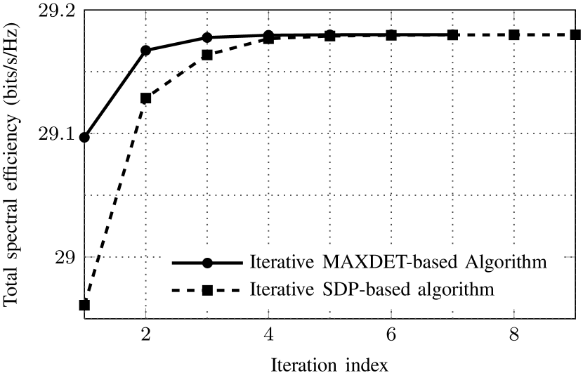
(a) Convergence rate for i.i.d channel realizations with $K_{\mathtt{D}}=K_{\mathtt{U}}=4$ and $N_{\mathtt{T}}=N_{\mathtt{R}}=4$.

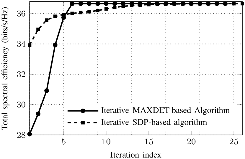
(b) Convergence rate for channel realizations taken from the channel model in Section IV-B. In this setup, $N_{\mathtt{T}}=4$, $N_{\mathtt{R}}=2$, $K_{\mathtt{D}}=6$, and $K_{\mathtt{U}}=4$.

Figure 2: Convergence rate of Algorithms 1 and 2 for a set of random channel realizations.

TABLE I: Average run time (in seconds) for i.i.d and realistic channel models for various simulation setups. The proposed algorithms terminate if the gap of the objectives between the last $10$ iterations is less than $\epsilon\leq 10^{-5}$.

$N_{\mathtt{T}}$			$2$	$4$	$6$	$8$	$10$	$12$
$N_{\mathtt{R}}=2$ $K_{\mathtt{D}}=2$ $K_{\mathtt{U}}=2$	i.i.d channel model	Algorithm 1 (SDPT3)	2.61	3.74	5.61	9.46	15.14	17.92
		Algorithm 2 (SeDuMi)	1.43	2.63	3.77	6.66	11.54	14.69
		Algorithm 2 (MOSEK)	0.089	0.26	0.45	1.09	2.68	3.38
	realistic channel model (given in Sec. IV-B)	Algorithm 1 (SDPT3)	4.17	6.28	9.29	15.04	23.76	28.51
		Algorithm 2 (SeDuMi)	2.36	4.13	6.11	10.50	17.64	22.93
		Algorithm 2 (MOSEK)	0.21	0.61	1.01	2.47	5.09	6.66
$K_{\mathtt{D}}$			$2$	$4$	$6$	$8$	$10$	$12$
$N_{\mathtt{T}}=4$ $N_{\mathtt{R}}=2$ $K_{\mathtt{U}}=2$	i.i.d channel model	Algorithm 1 (SDPT3)	3.74	9.64	13.01	16.27	18.76	25.32
		Algorithm 2 (SeDuMi)	2.63	6.25	8.12	9.98	12.77	15.96
		Algorithm 2 (MOSEK)	0.26	1.24	1.66	2.52	3.09	3.92
	realistic channel model (given in Sec. IV-B)	Algorithm 1 (SDPT3)	6.28	17.33	22.84	27.55	31.58	42.57
		Algorithm 2 (SeDuMi)	4.13	10.59	14.19	17.05	22.54	27.91
		Algorithm 2 (MOSEK)	0.61	2.24	2.90	4.34	5.24	7.08

IV-B Spectral Efficiency Performance

We now evaluate the performance of the full-duplex system for more realistic models. Particularly, we compare the achievable spectral efficiency of the proposed beamformer designs for the full-duplex system introduced in Section II with that of a traditional half-duplex scheme having the relevant hardware configurations. In fact, as mentioned earlier, the application with the most potential for full-duplex technology in cellular systems is in small cells. To quantify the potential benefit of the full-duplex transmission considered in this paper, we evaluate the performance of the proposed algorithms under the 3GPP LTE specifications for small cell deployments. The general simulation parameters are taken from [2, 42] and listed in Table II. Without loss of generality, per-user power constraints of users in the uplink transmission are assumed to be equal, i.e., $\overline{q}_{\mathtt{U}_{j}}=\overline{q}$. In particular, we consider two different settings of the transmit power constraints in both directions: (i) $(P_{\mathtt{BS}},\overline{q})=(26\;\textrm{dBm},23\;\textrm{dBm})$ following the LTE 3GPP pico cell standard for outdoor [2] and (ii) $(P_{\mathtt{BS}},\overline{q})=(10\;\textrm{dBm},10\;\textrm{dBm})$ according to the work of [7]. The number of antennas at the BS is set to $6$, of which $4$ are used for transmitting and $2$ for receiving, i.e., $N_{\mathtt{T}}=4$ and $N_{\mathtt{R}}=2$, respectively. All users in both directions are randomly dropped in a circle area of a radius $r=100$ m, centered at the full-duplex capable BS in an outdoor small cell scenario.

TABLE II: Simulation parameters

Carrier frequency	$2$GHz
System bandwidth	$10$MHz
Thermal noise	$-174$ dBm/Hz
Receiver noise figure (at downlink users)	$9$ dB
Receiver noise figure (at BS)	$5$ dB
Maximum transmit power at BS ($P_{\mathtt{BS}}$)	$10$ or $26$ dBm
Maximum transmit power per user ($\bar{q}$)	$10$ or $23$ dBm

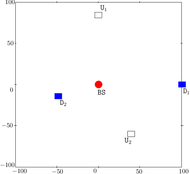
(a) Location of users of the simulation setup considered in Figs. 4 and 5

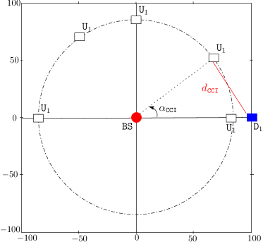
(b) Location of users of the simulation setup considered in Fig. 7

Figure 3: Location of users for the two specific simulation settings considered in the numerical results section.

The channel vector from the BS to $\mathtt{D}_{i}$ is given by $\mathbf{h}_{\mathtt{D}_{i}}=\sqrt{\kappa_{\mathtt{D}_{i}}}\tilde{\mathbf{h}}_{\mathtt{D}_{i}}$ where $\tilde{\mathbf{h}}_{\mathtt{D}_{i}}$ follows $\mathcal{CN}(0,\mathbf{I})$ that denotes the small scale fading, and $\kappa_{\mathtt{D}_{i}}=10^{(-\textrm{PL}_{\mathtt{LOS}}/10)}$ represents the path loss, where $\textrm{PL}_{\mathtt{LOS}}$ is calculated from a specific path loss model as shown in (45). The channel vector between the BS and $\mathtt{U}_{j}$ is generated in the same way. For large scale fading, we adopt the path loss model presented in [42, 2]. More specifically, downlink and uplink channels are assumed to experience the path loss model for line of sight (LOS) communications as

$$\begin{array}[]{rl}\textrm{PL}_{\mathtt{LOS}}&=103.8+20.9\log_{10}d\end{array}$$ (45)

where $\textrm{PL}_{\mathtt{LOS}}$ is in dB, $d$ is the distance (in kilometers) between the BS and a specific user. Similarly, the channel coefficient from $\mathtt{U}_{j}$ to $\mathtt{D}_{i}$ is modeled as $g_{ji}=\sqrt{\kappa_{ji}}\tilde{g}_{ji}$ where $\tilde{g}_{ji}$ follows $\mathcal{CN}(0,1)$ and $\kappa_{ji}=10^{(-\textrm{PL}_{\mathtt{NLOS}}/10)}$ denotes the large scale fading. Since there is a high possibility of obstructions between users deployed in an outdoor environment, we assume that the channel from $\mathtt{U}_{j}$ to $\mathtt{D}_{i}$ encounters the path loss model for non-line-of-sight (NLOS) transmission. That is, $\textrm{PL}_{\mathtt{NLOS}}$ (in dB) is written as

$$\textrm{PL}_{\mathtt{NLOS}}=145.4+37.5\log_{10}d_{\mathtt{CCI}}$$ (46)

where $d_{\mathtt{CCI}}$ is now the distance (in kilometers) from a user in the uplink transmission to another user in the downlink direction. The self-interference channel model is mentioned in Subsection IV-A.

To have a fair comparison between the full-duplex and half-duplex systems, we made the following assumptions. First, the BS of the half-duplex counterpart is assumed to use all antennas in both downlink and uplink transmissions, i.e., $N_{\mathtt{T}}+N_{\mathtt{R}}$. For the half-duplex case, since the downlink and uplink transmissions are separated, and thus the SEs of the downlink and uplink channels can be computed independently. Specifically, we use the iterative water-filling algorithm introduced in [43] to find the optimal SE of the uplink channel. Note that the problem of SE maximization in the downlink direction is NP-hard which requires extremely high computational complexity to find optimal solution [33]. Herein, we employ an efficient solution proposed in [23], which was shown to be close optimal, to calculate the SE of the downlink transmission. Then, the resulting SEs of the downlink and uplink channels in the half-duplex counterpart are divided by $2$ since each of them is assumed to share $50\%$ of the temporal resource [7]. For the full-duplex case, the SEs of the downlink and uplink channels are simply calculated by (3a) and (8a), respectively, after achieving the solutions of the problem in (10).

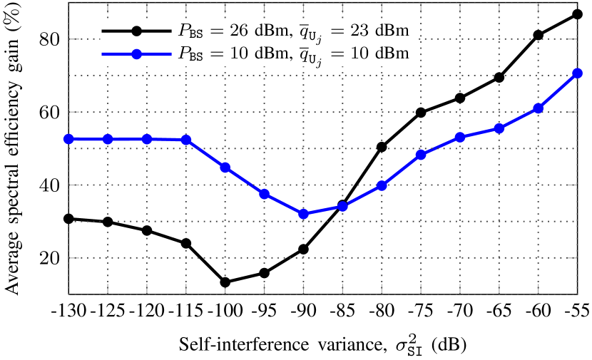
(a) Average spectral efficiency gain of downlink channel.

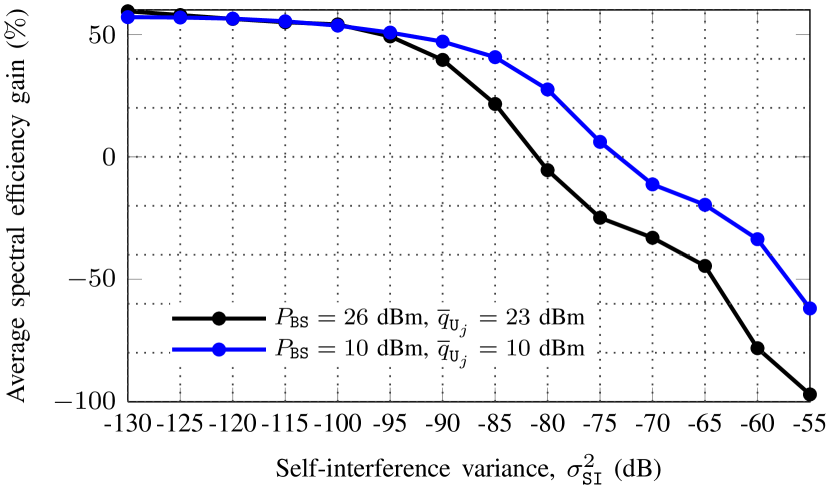
(b) Average spectral efficiency gain of uplink channel.

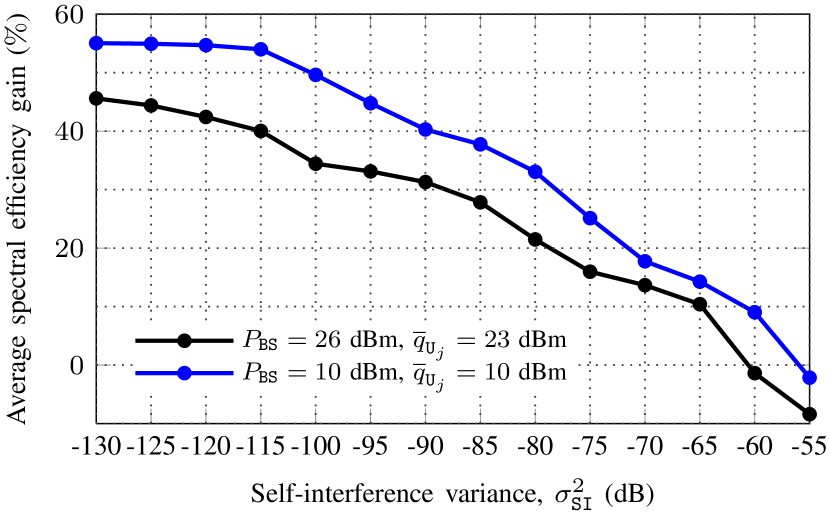
(c) Average spectral efficiency gain of entire system.

Figure 4: Average spectral efficiency gain ($\%$) versus $\sigma_{\mathtt{SI}}^{2}$ (dB) for the simulation scenario shown in Fig. 3(a).

Fig. 4 depicts the SE gains in percentage of the full-duplex system over the half-duplex one as a function of $\sigma_{\mathtt{SI}}^{2}$ for the scenario as shown in Fig. 3(a). A general observation is that full-duplex transmission can significantly improve the spectral efficiency of the half-duplex one when the self-interference is substantially suppressed. Specifically, as shown in Fig. 4(c), the total SE gain of the full-duplex system is $45.6\%$ and $55\%$ for the cases $(P_{\mathtt{BS}},\overline{q})=(26\;\textrm{dBm},23\;\textrm{dBm})$ and $(P_{\mathtt{BS}},\overline{q})=(10\;\textrm{dBm},10\;\textrm{dBm})$ at $\sigma_{\mathtt{SI}}^{2}=-130$ dB, respectively. However, when $\sigma_{\mathtt{SI}}^{2}=-55$ dB, the half-duplex system performs better than the full-duplex one for both cases of transmit power constraint. This observation simply means that the self-interference cancellation mechanism should be efficient enough for the full-duplex system to compete against the half-duplex counterpart. In addition, the simulation results also indicate that the self-interference needs to be canceled at least $75$ dB (i.e., $\sigma_{\mathtt{SI}}^{2}<-75$ dB) for the case $(P_{\mathtt{BS}},\overline{q})=(10\;\textrm{dBm},10\;\textrm{dBm})$ and at least $83$ dB (i.e., $\sigma_{\mathtt{SI}}^{2}<-83$ dB) for the case $(P_{\mathtt{BS}},\overline{q})=(26\;\textrm{dBm},23\;\textrm{dBm})$ for the full-duplex system to attain better SE in both downlink and uplink transmissions, compared to the half-duplex one. These requirements can be achieved by a recent advanced SI cancellation technique reported in [17].

To obtain more insights into the performance of the full-duplex system, we also study the gains of the downlink and uplink channels separately in Figs. 4(a) and 4(b), respectively. We can see that, while the SE of the uplink transmission of the full-duplex system is always deteriorated as $\sigma_{\mathtt{SI}}^{2}$ increases, that of the downlink channel decreases until a certain value of $\sigma_{\mathtt{SI}}^{2}$ ($-100$ dB and $-90$dB for $(P_{\mathtt{BS}},\overline{q})=(26\;\textrm{dBm},23\;\textrm{dBm})$ and $(P_{\mathtt{BS}},\overline{q})=(10\;\textrm{dBm},10\;\textrm{dBm})$, respectively) and increases after that. The degradation on the SE of the uplink channel is obvious and due to the fact that a large value of $\sigma_{\mathtt{SI}}^{2}$ results in a greater amount of self-interference power being added to the background noise. To explain different trends in the SE of the downlink channel, we first recall that the main goal of the proposed designs is to maximize the total SE of the full-duplex system, i.e., jointly optimizing both uplink and downlink transmissions. When the SI is quite small, the joint optimization schemes slightly reduce the actual transmit power of the downlink channel to maintain the SE of the uplink channel. For a large value of $\sigma_{\mathtt{SI}}^{2}$, the self-interference is comparable or even dominates the desired signals of the users in the uplink channel. Hence, data detection for uplink users becomes more erroneous, incredibly deteriorating the uplink performance. For such a case, the total SE of the full-duplex system is mostly determined by the downlink transmission since the SE of the uplink channel is extremely low. Thus, it is better to reduce the transmit power in the uplink channel and concentrate on maximizing the SE of the downlink channel. As a result, the SE of the uplink channel greatly declined. Specifically, the SE of the uplink direction of the full-duplex system is remarkably smaller than that of the half-duplex one as $\sigma_{\mathtt{SI}}^{2}\geq-80$ and $\sigma_{\mathtt{SI}}^{2}\geq-70$ for $(P_{\mathtt{BS}},\overline{q})=(26\;\textrm{dBm},23\;\textrm{dBm})$ and $(P_{\mathtt{BS}},\overline{q})=(10\;\textrm{dBm},10\;\textrm{dBm})$, respectively. It is worth noting that a reduction in the transmit power of users in uplink channel results in a decrease in the CCI. This explains the increment of the SE gain in the downlink transmission as $\sigma_{\mathtt{SI}}^{2}$ is greater than a certain threshold. An interesting observation from Fig. 4(c) is that the SE gain of the full-duplex system is higher when the maximum transmit power is smaller. This is due to the fact that smaller maximum transmit powers create a smaller amount of self-interference as well as CCI.

In Fig. 5, we show cumulative distribution function (CDF) of the total SE gain of the full-duplex for the scenario in Fig. 3(a). Obviously, for the same power setting, a smaller value of $\sigma_{\mathtt{SI}}^{2}$ results in better SE gain. On the other hand, for the same $\sigma_{\mathtt{SI}}^{2}$, a lower transmit power yields better SE gain. These observations are consistent with the observation in Fig. 4(c).

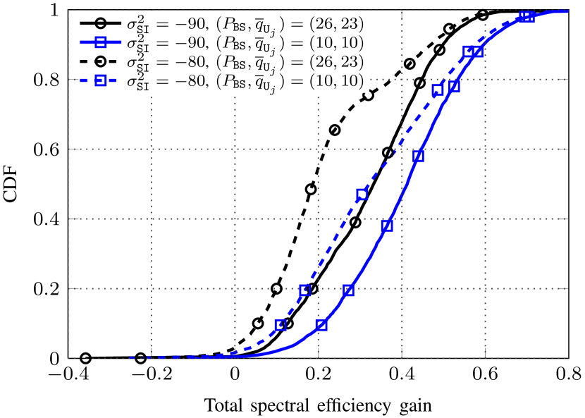
Figure 5: CDF of total spectral efficiency gains for $5000$ random channel realizations for the scenario shown in Fig. 3(a). The unit of $\sigma_{\mathtt{SI}}^{2}$ is dB and that of $P_{\mathtt{BS}}$ and $\overline{q}$ is dBm.

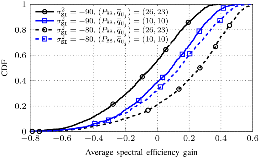
(a) CDF of average spectral efficiency gain of downlink channel.

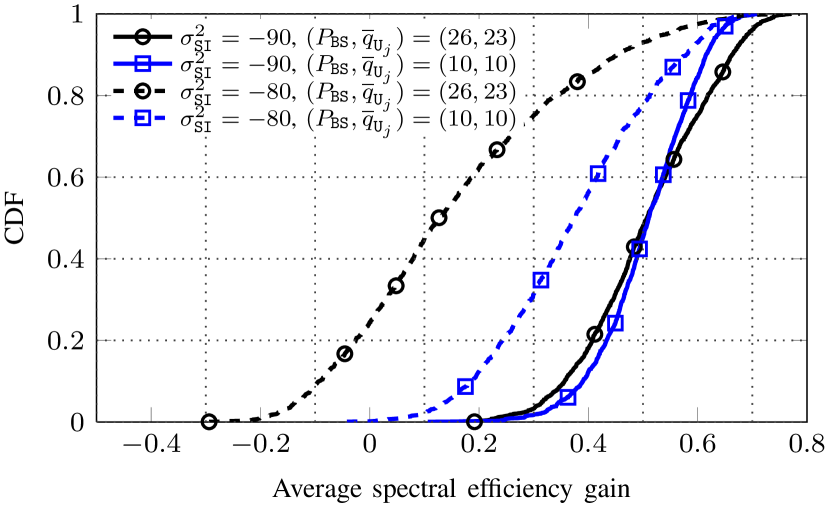
(b) CDF of average spectral efficiency gain of uplink channel.

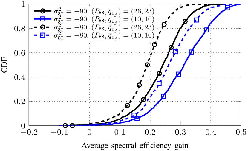
(c) CDF of average spectral efficiency gain of entire system.

Figure 6: CDF of average spectral efficiency gains for $1000$ random topologies. The simulation scenario parameters are $K_{\mathtt{D}}=K_{\mathtt{U}}=2$, $N_{\mathtt{T}}=4$ and $N_{\mathtt{R}}=2$. The users are uniformly dropped in a circle area of a radius $r=100$ meters centered at the BS at random. The unit of $\sigma_{\mathtt{SI}}^{2}$ is dB and that of $P_{\mathtt{BS}}$ and $\overline{q}$ is dBm.

The performance of the full-duplex is further explored in the next numerical experiment, in which we study the CDF of the average SE gain of the full-duplex system for a number of random topologies. The results in Fig. 6 are plotted for $1000$ topologies, where all users are uniformly distributed in a circle area of a radius $r=100$ meters centered at the BS. For each topology, the spectral efficiency gain is averaged over $500$ random channel realizations. As can be seen in Fig. 6(c), the total average SE of full-duplex systems are higher than that of the half-duplex one for most of the topologies. For example, the SE gains are larger than $20\%$ and $28\%$ for the power settings $(P_{\mathtt{BS}},\overline{q})=(26\;\textrm{dBm},23\;\textrm{dBm})$ and $(P_{\mathtt{BS}},\overline{q})=(10\;\textrm{dBm},10\;\textrm{dBm})$, respectively for a half of the simulated topologies at $\sigma_{\mathtt{SI}}^{2}=-80$ dB. Not surprisingly, the SE gain of the downlink channel is rather sensitive to topologies which determine the degree of CCI. On the other hand, positions of users have a small impact on the SE of the uplink transmission when $\sigma_{\mathtt{SI}}^{2}=-90$ dB. The reason is that the self-interference in this case is relatively lower than the received signal strength for most of the topologies. However, the situation dramatically changes as $\sigma_{\mathtt{SI}}^{2}$ increases to $-80$ dB, where more dependency between topology and SE gain is observed. Thus, the number of scenarios that can yield a received signal strength higher than the SI power is reduced for a larger value of $\sigma_{\mathtt{SI}}^{2}$.

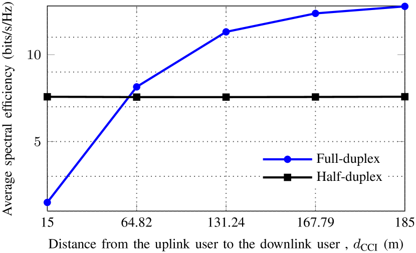
(a) Average spectral efficiency of downlink channel.

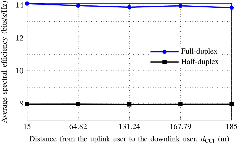
(b) Average spectral efficiency of uplink channel.

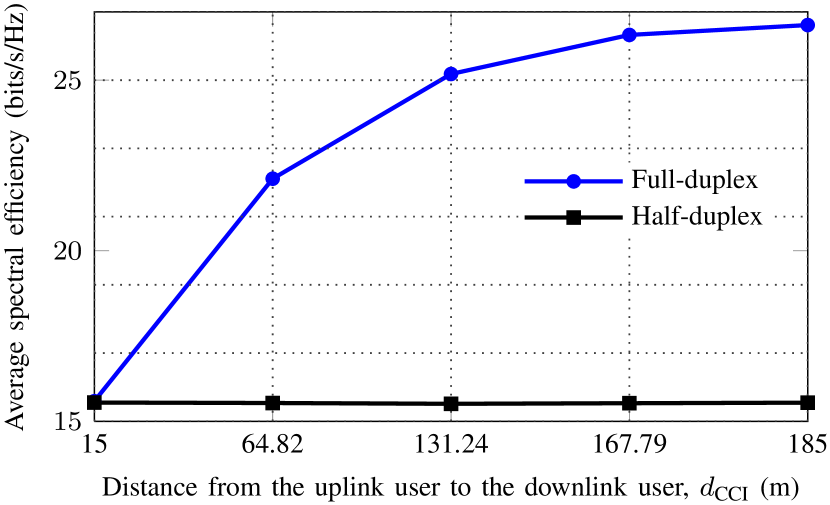
(c) Average spectral efficiency of entire system.

Figure 7: Average spectral efficiency versus distance from the uplink user to downlink one, $d_{\mathtt{CCI}}$. In this setup, $\sigma_{\mathtt{SI}}^{2}=-100$ dB, $P_{\mathtt{BS}}=26$ dBm and $\overline{q}_{\mathtt{U}_{j}}=23$ dBm. The distance of the BS and users, i.e., $\mathtt{D}_{1}$, and $\mathtt{U}_{1}$ are set at $r$ and $0.85r$, respectively. The position of $\mathtt{D}_{1}$ is fixed while $\mathtt{U}_{1}$ moves on a circle with radius $0.85r$ as shown in Fig. 3(b).

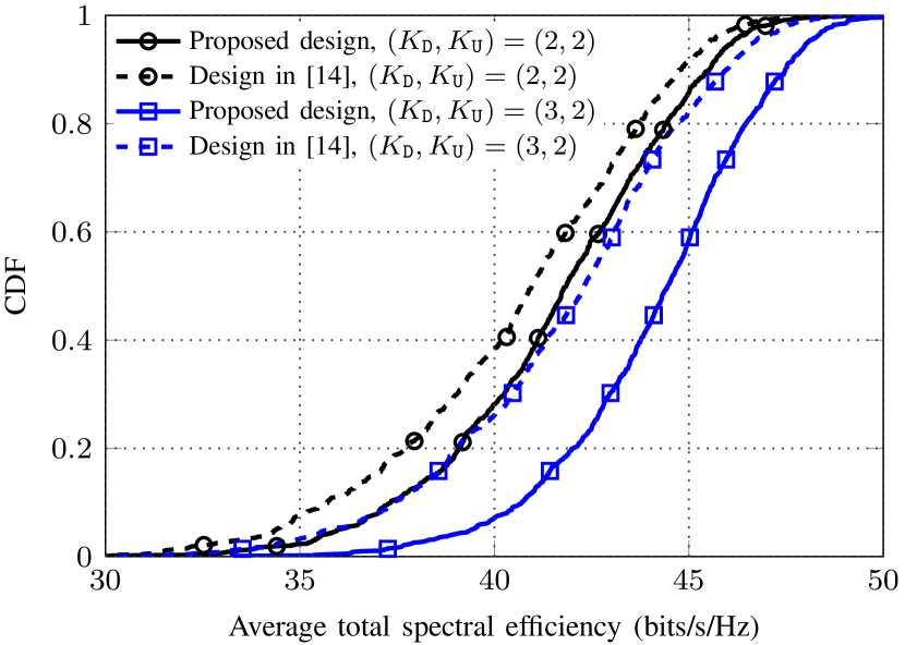
Figure 8: CDF of average total spectral efficiency of the proposed design and the design with no consideration of CCI in [14] for $1000$ random topologies. In the simulation setting, $\sigma_{\mathtt{SI}}^{2}=-100$ dB, $P_{\mathtt{BS}}=26$ dBm and $\overline{q}_{\mathtt{U}_{j}}=23$ dBm.

Next, we study the impact of co-channel interference on the SE of the full-duplex system. For this purpose, we fix $\sigma_{\mathtt{SI}}^{2}$ at $-100$ dB, and consider a setting shown in Fig. 3(b). In this simulation setup, we vary the distance between $\mathtt{U}_{1}$ and $\mathtt{D}_{1}$, denoted by $d_{\mathtt{CCI}}$, and plot the resulting SEs of the full-duplex system in Fig. 7. Each value of $d_{\mathtt{CCI}}$ on the x-axis of Fig. 7 corresponds to a position of $\mathtt{U}_{1}$, while $\mathtt{D}_{1}$ is held fixed. We observe that the spectral efficiency of $\mathtt{D}_{1}$ increases as $\mathtt{U}_{1}$ moves far away from $\mathtt{D}_{1}$. Especially when the two users are close (e.g., $d_{\mathtt{CCI}}<64.82$ m), the performance of the full-duplex downlink transmission can be worse than that of the half-duplex one. The reason is straightforward since decreasing $d_{\mathtt{CCI}}$ leads to an increase in CCI which then degrades the SE of the downlink channel. On the other hand, the location of $\mathtt{U}_{1}$ has a small impact on the SE of the uplink transmission for a fixed small value of $\sigma_{\mathtt{SI}}^{2}$. The results in Fig. 7 indicate that the CCI is a critical factor that needs to be controlled for successful deployment of full-duplex systems.

In the final numerical experiment we plot the CDF of the average total SE of the full-duplex system with and without accounting for the CCI. The problem of beamformer design without taking CCI into account was studied in [14]. The curves in Fig. 8 are obtained from 1000 random topologies. For each topology, the average total SE is calculated over $500$ random channel realizations. It is obvious that the proposed designs in this paper outperform the one with no CCI in [14] as expected. For instance, the proposed designs attain 2 bits/s/Hz of total SE higher than the scheme in [14] for approximately $60\%$ of the simulated topologies when $K_{\mathtt{D}}=3$ and $K_{\mathtt{U}}=2$. As the total number of users is reduced, the SE becomes smaller due to a decrease in the available multiuser diversity gain.

V Conclusion and Future Work

In this paper we have devised a beamforming scheme for a full-duplex system, in which a full-duplex capable BS communicates with multiple half-duplex users in the downlink and uplink channels simultaneously. In particular, we have considered the problem of joint SE maximization of downlink and uplink transmissions under some power constraints. First, the design problem is formulated as a rank constrained optimization one, and then the rank relaxation technique is applied. However, the relaxed problem is still nonconvex. To solve this problem we have proposed two iterative algorithms, one based on the concept of the FW algorithm and the other based on the framework of SPCA method. The idea of both proposed methods is to approximate the nonconvex problem by a convex formulation in each iteration. While the first approach needs to solve a sequence of MAXDET programs, the second one relies on solving a series of SDPs. We have carried out several numerical experiments under 3GPP LTE small cell setups to evaluate the SE performance of the full-duplex scheme. It has been shown that the SE of the full-duplex system is remarkably larger than that of the half-duplex one as the capability of current SI cancellation schemes is efficient. Our work has proved that the full-duplex transmission is a promising technique to improve the SE of small cell wireless communications systems.

The work considered in this paper also opens several possibilities for future research. First, more efficient designs of self-interference cancellation for full-duplex MIMO systems are of critical importance. In addition to distributed algorithms for multiple small cell setups as mentioned earlier, a mechanism which can accurately measure the CCI at users in the downlink channel is required. When many users are active in the downlink and uplink channels, a CCI-aware user scheduling scheme which can control the CCI is a good solution to the full-duplex systems. This allows us to exploit the multiuser-diversity gain in both directions. Furthermore, since the uplink performance of the full-duplex system is significantly reduced, even worse than the half-duplex one due to a large amount of self-interference, a mechanism to control the fairness among users needs to be proposed. For example, we can additionally impose a rate constraint on the SE of the uplink channel. The future research can also include an efficient algorithm to switch between full-duplex and half-duplex systems. Since the downlink and uplink channels operate at the same time, some traditional MAC protocols, which are dedicated to current half-duplex systems, need to be redesigned. These interesting problems call for more comprehensive studies, and thus are beyond the scope of this paper.

[Proof of Convergence]

In this appendix we adopt the techniques from [31] to prove the convergence of Algorithms 1 and 2 (i.e., the iterative MAXDET-based algorithm and the iterative SDP-based algorithm, respectively) to a KKT point. Let us start with the convergence proof of Algorithm 1. First, we note that the affine majorization in (14) has the following two important properties which are the key to show the convergence to a KKT point of Algorithm 1

$$g^{(n)}(\mathbf{Q}^{(n)},\mathbf{q}^{(n)}) = g(\mathbf{Q}^{(n)},\mathbf{q}^{(n)}),$$ (47)

$$\nabla g^{(n)}(\mathbf{Q}^{(n)},\mathbf{q}^{(n)}) = \nabla g(\mathbf{Q}^{(n)},\mathbf{q}^{(n)})$$ (48)

where property (47) means that the inequality in (14) is tight when $(\mathbf{Q},\mathbf{q})=(\mathbf{Q}^{(n)},\mathbf{q}^{(n)})$ and property (48) is obvious due to the first order approximation. Note that the gradient in (48) is with respect to $\mathbf{Q}$ and $q$. To proceed further, let $\mathcal{S}$ denote the feasible set of (17), i.e., the set of $\mathbf{Q}$ and $\mathbf{q}$ that satisfy the constraint (10e), (10e) and (10e). We note that $\mathcal{S}$ is a compact convex set. Further let $u^{(n+1)}$ be is the obtained optimal objective of (17) at iteration $n+1$. According to the updating rule in Algorithm 1, we can derive the following inequalities

$$u^{(n+1)} = h(\mathbf{Q}^{(n+1)},\mathbf{q}^{(n+1)})-g^{(n)}(\mathbf{Q}^{(n+1)},\mathbf{q}^{(n+1)})$$ (49)

$$= \underset{(\mathbf{Q},\mathbf{q})\in\mathcal{S}}{\max}\ h(\mathbf{Q},\mathbf{q})-g^{(n)}(\mathbf{Q},\mathbf{q})$$ (50)

$$\geq h(\mathbf{Q}^{(n)},\mathbf{q}^{(n)})-g^{(n)}(\mathbf{Q}^{(n)},\mathbf{q}^{(n)})$$ (51)

$$= h(\mathbf{Q}^{(n)},\mathbf{q}^{(n)})-g(\mathbf{Q}^{(n)},\mathbf{q}^{(n)})$$ (52)

$$\geq h(\mathbf{Q}^{(n)},\mathbf{q}^{(n)})-g^{(n-1)}(\mathbf{Q}^{(n)},\mathbf{q}^{(n)})=u^{(n)}$$ (53)

where (51) follows from the fact that the objective at the optimal solution is greater than the one at any feasible solution, i.e., $f(\mathbf{x}^{\star})=\underset{\mathbf{x}\in\mathcal{X}}{\max}f(\mathbf{x})\geq f(\mathbf{x}_{0})$ where $\mathbf{x}^{\star}$ and $\mathbf{x}_{0}$ are an optimal solution and any feasible solution, respectively, (52) is due to (47), (53) is due to the affine majorization in (14). In fact, we have shown that the sequence $\{u^{(n)}\}$ in nondecreasing. Furthermore, the value of $\{u^{(n)}\}$ is bounded above due to the limited transmit power, and thus it is guaranteed to converge. We note that the function $f(\mathbf{X})=\log\det(\mathbf{X})$ is differentiable and strictly concave on $\mathbf{X}\succ\mathbf{0}$ [34, Section 3.1]. Since $\mathcal{S}$ is a compact convex set, the objective is then shown to be strongly concave on $\mathcal{S}$ due to [31, Lemma 3.1]. As a result, the sequence $(\mathbf{Q}^{(n)},\mathbf{q}^{(n)})$ converges to an accumulation point denoted by $(\mathbf{Q}^{\ast},\mathbf{q}^{\ast})$. To establish the convergence to a KKT point, we first introduce the set of dual variables for the constraints in (17) which is listed in Table III.

TABLE III: Constraints and their corresponding dual variables

Constraints	Dual variables
$0\leq q_{\mathtt{U}_{j}}$	$\lambda_{\mathtt{U}_{j}}$
$q_{\mathtt{U}_{j}}\leq\overline{q}_{\mathtt{U}_{j}}$	$\tilde{\lambda}_{\mathtt{U}_{j}}$
$\sum_{i=1}^{K_{\mathtt{D}}}\operatorname{Tr}(\mathbf{Q}_{\mathtt{D}_{i}})\leq P_{\mathtt{BS}}$	$\mu$
$\mathbf{Q}_{\mathtt{D}_{i}}\succeq 0$	$\mathbf{Z}_{\mathtt{D}_{i}}$

It is easy to check that the Slater’s condition holds for the convex program at all iterations of Algorithm 1. Thus, the KKT conditions are necessary and sufficient for optimality [34, Section 5.5]. With the dual variables introduced in Table III, the KKT conditions of the optimal value at iteration $n$ (see [34] for more details) are given as

$$\nabla_{\mathbf{Q}_{\mathtt{D}_{i}}}h(\mathbf{Q}^{(n)},\mathbf{q}^{(n)})-\nabla_{\mathbf{Q}_{\mathtt{D}_{i}}}g^{(n)}(\mathbf{Q}^{(n)},\mathbf{q}^{(n)})\\ -\mu\mathbf{I}+\mathbf{Z}_{\mathtt{D}_{i}}\;=\;\mathbf{0},\ \forall i=1,\ldots,K_{\mathtt{D}},$$ (54)

$$\partial_{q_{\mathtt{U}_{j}}}h(\mathbf{Q}^{(n)},\mathbf{q}^{(n)})-\partial_{q_{\mathtt{U}_{j}}}g^{(n)}(\mathbf{Q}^{(n)},\mathbf{q}^{(n)})\\ +\lambda_{\mathtt{U}_{j}}-\tilde{\lambda}_{\mathtt{U}_{j}}\;=\;0,\ \forall j=1,\ldots,K_{\mathtt{U}},$$ (55)

$$\lambda_{\mathtt{U}_{j}}q_{\mathtt{U}_{j}}^{(n)}=0;\ \tilde{\lambda}_{\mathtt{U}_{j}}(q_{\mathtt{U}_{j}}^{(n)}-\overline{q}_{\mathtt{U}_{j}})=0,\ \forall j=1,\ldots,K_{\mathtt{U}},$$ (56)

$$\operatorname{Tr}(\mathbf{Q}_{\mathtt{D}_{i}}^{(n)}\mathbf{Z}_{\mathtt{D}_{i}})=0,\ \forall i=1,\ldots,K_{\mathtt{D}},$$ (57)

$$\mu\bigl{(}\sum_{i=1}^{K_{\mathtt{D}}}\operatorname{Tr}(\mathbf{Q}_{\mathtt{D}_{i}}^{(n)})-P_{\mathtt{BS}}\bigr{)}=0.$$ (58)

Due to property (48), we can replace $\nabla_{\mathbf{Q}_{\mathtt{D}_{i}}}g^{(n)}(\mathbf{Q}^{(n)},\mathbf{q}^{(n)})$ and $\partial_{q_{\mathtt{U}_{j}}}g^{(n)}(\mathbf{Q}^{(n)},\mathbf{q}^{(n)})$ by $\nabla_{\mathbf{Q}_{\mathtt{D}_{i}}}g(\mathbf{Q}^{(n)},\mathbf{q}^{(n)})$ and $\partial_{q_{\mathtt{U}_{j}}}g(\mathbf{Q}^{(n)},\mathbf{q}^{(n)})$ on convergence (i.e., as $n\to\infty$), respectively. Thus,

$$\nabla_{\mathbf{Q}_{\mathtt{D}_{i}}}h(\mathbf{Q}^{(n)},\mathbf{q}^{(n)})-\nabla_{\mathbf{Q}_{\mathtt{D}_{i}}}g(\mathbf{Q}^{(n)},\mathbf{q}^{(n)})\\ -\mu\mathbf{I}+\mathbf{Z}_{\mathtt{D}_{i}}\;=\;\mathbf{0},\ \forall i=1,\ldots,K_{\mathtt{D}},$$ (59)

$$\partial_{q_{\mathtt{U}_{j}}}h(\mathbf{Q}^{(n)},\mathbf{q}^{(n)})-\partial_{q_{\mathtt{U}_{j}}}g(\mathbf{Q}^{(n)},\mathbf{q}^{(n)})\\ +\lambda_{\mathtt{U}_{j}}-\tilde{\lambda}_{\mathtt{U}_{j}}\;=\;0,\ \forall j=1,\ldots,K_{\mathtt{U}}.$$ (60)

It is straightforward to see that the set of equations in (56)-(60) are actually the KKT conditions for the problem (13) and thus completes the proof. We note that the KKT conditions for the convex program after convergence are also the necessary ones for local optimality of the problem (13). Indeed since $(\mathbf{Q}^{\ast},\mathbf{q}^{\ast})$ is an optimal solution to the convex program at convergence, it satisfies [44, Section 2.1]

$$\bigl{\langle}\nabla g^{(\infty)}(\mathbf{Q}^{\ast},\mathbf{q}^{\ast})-\nabla h(\mathbf{Q}^{\ast},\mathbf{q}^{\ast}),(\mathbf{Q}^{\prime},\mathbf{q}^{\prime})\\ -(\mathbf{Q}^{\ast},\mathbf{q}^{\ast})\bigr{\rangle}\geq 0\ \text{for all}\ (\mathbf{Q}^{\prime},\mathbf{q}^{\prime})\in\mathcal{S}$$ (61)

where $\left\langle,\right\rangle$ stands for the inner product of the arguments, i.e., $\bigl{\langle}\mathbf{X},\mathbf{Y}\bigr{\rangle}=\operatorname{Tr}(\mathbf{X}^{H}\mathbf{Y})$, the subtraction in (61) is element-wise, and the gradient is with respect to $\mathbf{Q}$ and $\mathbf{q}$. As mentioned previously, we can replace $\nabla g^{(\infty)}(\mathbf{Q}^{\ast},\mathbf{q}^{\ast})$ by $\nabla g(\mathbf{Q}^{\ast},\mathbf{q}^{\ast})$, and thus (61) becomes

$$\bigl{\langle}\nabla g(\mathbf{Q}^{\ast},\mathbf{q}^{\ast})-\nabla h(\mathbf{Q}^{\ast},\mathbf{q}^{\ast}),(\mathbf{Q}^{\prime},\mathbf{q}^{\prime})\\ -(\mathbf{Q}^{\ast},\mathbf{q}^{\ast})\bigr{\rangle}\geq 0\ \text{for all}\ (\mathbf{Q}^{\prime},\mathbf{q}^{\prime})\in\mathcal{S}$$ (62)

which is the first order necessary conditions for local optimality of the problem (13) [44, Section 2.1].

The proof of Algorithm 2 follows the same spirit. As mentioned earlier for the convex approximation in (32), $F(t_{\mathtt{D}_{i}},\beta_{\mathtt{D}_{i}},\psi_{\mathtt{D}_{i}}^{(n)})=f(t_{\mathtt{D}_{i}},\beta_{\mathtt{D}_{i}})$ when $\psi_{\mathtt{D}_{i}}^{(n)}=t_{\mathtt{D}_{i}}/\beta_{\mathtt{D}_{i}}$, that is

$$F(t_{\mathtt{D}_{i}},\beta_{\mathtt{D}_{i}},\psi_{\mathtt{D}_{i}}^{(n)})|_{\psi_{\mathtt{D}_{i}}^{(n)}=t_{\mathtt{D}_{i}}/\beta_{\mathtt{D}_{i}}}=t_{\mathtt{D}_{i}}\beta_{\mathtt{D}_{i}}=f(t_{\mathtt{D}_{i}},\beta_{\mathtt{D}_{i}}).$$ (63)

Furthermore, we also have

$$\begin{array}[]{rl}\left.\frac{\partial F(t_{\mathtt{D}_{i}},\beta_{\mathtt{D}_{i}},\psi_{\mathtt{D}_{i}}^{(n)})}{\partial t_{\mathtt{D}_{i}}}\right|_{\psi_{\mathtt{D}_{i}}^{(n)}=t_{\mathtt{D}_{i}}/\beta_{\mathtt{D}_{i}}}&=\left.{\displaystyle\frac{1}{\psi_{\mathtt{D}_{i}}^{(n)}}}t_{\mathtt{D}_{i}}\right|_{\psi_{\mathtt{D}_{i}}^{(n)}=t_{\mathtt{D}_{i}}/\beta_{\mathtt{D}_{i}}}\\ \\ &=\beta_{\mathtt{D}_{i}}={\displaystyle\frac{\partial f(t_{\mathtt{D}_{i}},\beta_{\mathtt{D}_{i}})}{\partial t_{\mathtt{D}_{i}}}}\end{array}$$ (64)

and

$$\left.\frac{\partial F(t_{\mathtt{D}_{i}},\beta_{\mathtt{D}_{i}},\psi_{\mathtt{D}_{i}}^{(n)})}{\partial\beta_{\mathtt{D}_{i}}}\right|_{\psi_{\mathtt{D}_{i}}^{(n)}=t_{\mathtt{D}_{i}}/\beta_{\mathtt{D}_{i}}}=\frac{\partial f(t_{\mathtt{D}_{i}},\beta_{\mathtt{D}_{i}})}{\partial\beta_{\mathtt{D}_{i}}}.$$ (65)

Let $\mathcal{S}^{(n)}$ be the feasible set of the convex program solved at iteration $n$. Due to the updating rule in Algorithm 2 (i.e., $\psi_{\mathtt{D}_{i}}^{(n+1)}=t_{\mathtt{D}_{i}}^{(n)}/\beta_{\mathtt{D}_{i}}^{(n)}$), follows that $F(t_{\mathtt{D}_{i}}^{(n)},\beta_{\mathtt{D}_{i}}^{(n)},\psi_{\mathtt{D}_{i}}^{(n+1)})=f(t_{\mathtt{D}_{i}}^{(n)},\beta_{\mathtt{D}_{i}}^{(n)})$. Similarly, we have $G\bigl{(}x_{\mathtt{U}_{j}},\mathbf{Q},\mathbf{q},x_{\mathtt{U}_{j}}^{(n)},\mathbf{Q}^{(n)},\mathbf{q}^{(n)}\bigr{)}=-g(x_{\mathtt{U}_{j}}^{(n)},\mathbf{Q}^{(n)},\mathbf{q}^{(n)})$. This means that $(x_{\mathtt{U}_{j}}^{(n)},\mathbf{Q}^{(n)},\mathbf{q}^{(n)})\in\mathcal{S}^{(n+1)}$ and thus $u^{(n+1)}\geq u^{(n)}$ where $u^{(n)}$ is the objective of (19a) at iteration $n$. The convergence proof to a solution that satisfies KKT conditions follows the same steps from (49) to (60) presented above.

References

• [1] E. Telatar, “Capacity of multi-antenna gaussian channels,” Eur. Trans. Telecommun., vol. 10, pp. 585–595, Nov. 1999.
• [2] 3GPP Technical Specification Group Radio Access Network, Evolved Universal Terrestrial Radio Access (E-UTRA): Further advancements for E-UTRA physical layer aspects (Release 9), 3GPP Std. TS 36.814 V9.0.0, 2010.
• [3] Part 16: Air Interface for Broadband Wireless Access Systems, IEEE Std. 802.16-2009, 2009.
• [4] J. I. Choi, M. Jain, K. Srinivasan, P. Levis, and S. Katti, “Achieving single channel, full duplex wireless communication,” in Proc. MOBICOM’10, Chicago, USA, Sep. 2010, pp. 1–12.
• [5] M. Jain, J. I. Choi, T. Kim, D. Bharadia, S. Seth, K. Srinivasan, P. Levis, S. Katti, and P. Sinha, “Practical, real-time, full duplex wireless,” in Proc. MOBICOM’11, Las Vegas, USA, Sep. 2011, pp. 301–312.
• [6] M. Duarte and A. Sabharwal, “Full-duplex wireless communications using off-the-shelf radios: feasibility and first results,” in Proc. Asilomar Conf. Signals Syst. Comput. (ASILOMAR), California, USA, Nov. 2010, pp. 1558–1562.
• [7] M. Duarte, C. Dick, and A. Sabharwal, “Experiment-driven characterization of full-duplex wireless systems,” IEEE Trans. Wireless Commun., vol. 11, no. 12, pp. 4296–4307, Dec. 2012.
• [8] J. I. Choi, S. Hong, M. Jain, S. Katti, P. Levis, and J. Mehlman, “Beyond full duplex wireless,” in Proc. Asilomar Conf. Signals Syst. Comput. (ASILOMAR), California, USA, Nov. 2012, pp. 40–44.
• [9] Dan Nguyen, L.-N. Tran, P. Pirinen, and M. Latva-aho, “Transmission strategies for full duplex multiuser MIMO systems,” in Proc. the International Workshop on Small Cell Wireless Networks, IEEE ICC 2012, Jun. 2012, pp. 6825–6829.
• [10] J.-H. Lee and O.-S. Shin, “Distributed beamforming approach to full-duplex relay in multiuser MIMO transmission,” in Proc. WCNC 2012 Workshop on 4G Mobile Radio Access networks, Apr. 2012, pp. 278–282.
• [11] B. Day, A. Margetts, D. Bliss, and P. Schniter, “Full-Duplex Bidirectional MIMO: Achievable Rates Under Limited Dynamic Range,” IEEE Trans. Signal Process., vol. 60, no. 7, pp. 3702–3713, 2012.
• [12] G. Zheng, I. Krikidis, and B. Ottersten, “Full-duplex cooperative cognitive radio with transmit imperfections,” IEEE Trans. Wireless Commun., vol. 12, no. 5, pp. 2498–2511, May 2013.
• [13] E. Aryafar, M. A. Khojastepour, K. Sundaresan, S. Rangarajan, and M. Chiang, “MIDU: enabling MIMO full duplex,” in Proc. MOBICOM’12, Istanbul, Turkey, 2012, pp. 257–268.
• [14] Dan Nguyen, L.-N. Tran, P. Pirinen, and M. Latva-aho, “Precoding for Full Duplex Multiuser MIMO Systems: Spectral and Energy Efficiency Maximization,” IEEE Trans. Signal Process., vol. 61, no. 16, pp. 4038–4050, 2013.
• [15] “System Scenarios and Technical Requirements for Full-Duplex Concept,” DUPLO project, Deliverable D1.1. [Online]. Available: http://www.fp7-duplo.eu/index.php/deliverables
• [16] The Duplo website. [Online]. Available: http://www.fp7-duplo.eu/
• [17] D. Bharadia, E. McMilin, and S. Katti, “Full duplex radios,” in Proc. SIGCOMM’13, Aug. 2013, pp. 375–386.
• [18] D. W. K. Ng, E. S. Lo, and R. Schober, “Dynamic Resource Allocation in MIMO-OFDMA Systems with Full-Duplex and Hybrid Relaying,” IEEE Trans. Commun., vol. 60, no. 5, pp. 1291–1304, 2012.
• [19] B. Day, A. Margetts, D. Bliss, and P. Schniter, “Full-duplex MIMO relaying: Achievable rates under limited dynamic range,” IEEE J. Sel. Areas Commun., vol. 30, no. 8, pp. 1541–1553, 2012.
• [20] H. Weingarten, Y. Steinberg, and S. Shamai, “The capacity region of the Gaussian multiple-input multiple-output broadcast channel,” IEEE Trans. Inf. Theory, vol. 52, no. 9, pp. 3936–3964, Sep. 2006.
• [21] M. Bengtsson and B. Ottersten, “Optimal and suboptimal transmit beamforming,” in Handbook of Antennas in Wireless Communications, L. C. E. Godara, Ed.   CRC Press, 2001.
• [22] A. Gershman, N. Sidiropoulos, S. Shahbazpanahi, M. Bengtsson, and B. Ottersten, “Convex optimization-based beamforming,” IEEE Signal Processing Magazine, vol. 27, no. 3, pp. 62–75, 2010.
• [23] L.-N. Tran, M. F. Hanif, A. Tölli, and M. Juntti, “Fast converging algorithm for weighted sum rate maximization in multicell MISO downlink,” IEEE Signal Process. Lett., vol. 19, no. 12, pp. 872–875, Dec. 2012.
• [24] D. Tse and P. Viswanath, Fundamentals of Wireless Communication.   Cambridge University Press, 2005.
• [25] N. Sidiropoulos, T. Davidson, and Z.-Q. Luo, “Transmit beamforming for physical-layer multicasting,” IEEE Trans. Signal Process., vol. 54, no. 6, pp. 2239–2251, Jun. 2006.
• [26] Z.-Q. Luo, W.-K. Ma, A.-C. So, Y. Ye, and S. Zhang, “Semidefinite relaxation of quadratic optimization problems,” IEEE Signal Process. Mag., vol. 27, no. 3, pp. 20–34, May 2010.
• [27] A. Wiesel, Y. Eldar, and S. Shamai, “Zero-forcing precoding and generalized inverses,” IEEE Trans. Signal Process., vol. 56, no. 9, pp. 4409 –4418, 2008.
• [28] L.-N. Tran, M. Juntti, M. Bengtsson, and B. Ottersten, “Beamformer designs for MISO broadcast channels with zero-forcing dirty paper coding,” IEEE Trans. Wireless Commun., vol. 12, no. 3, pp. 1173–1185, Mar. 2013.
• [29] ——, “Weighted sum rate maximization for MIMO broadcast channels using dirty paper coding and zero-forcing methods,” IEEE Trans. Commun., vol. 61, no. 6, pp. 2362–2373, Jun. 2013.
• [30] M. Frank and P. Wolfe, “An algorithm for quadratic programming,” Naval Research Logistics Quarterly, vol. 3, no. 1-2, pp. 95–110, 1956.
• [31] A. Beck, A. Ben-Tal, and L. Tetruashvili, “A sequential parametric convex approximation method with applications to nonconvex truss topology design problems,” Journal of Global Optimization, vol. 47, no. 1, pp. 29–51, 2010.
• [32] L.-N. Tran, “An iterative precoder design for successive zero-forcing precoded systems,” IEEE Commun. Lett., vol. 16, no. 1, pp. 16–18, Jan. 2012.
• [33] Z.-Q. Luo and S. Zhang, “Dynamic spectrum management: Complexity and duality,” IEEE J. Sel. Topics Signal Process., vol. 2, no. 1, pp. 57–73, Feb. 2008.
• [34] S. Boyd and L. Vandenberghe, Convex Optimization.   Cambridge University Press, 2004.
• [35] J. Dattorro, Convex Optimization & Euclidean Distance Geometry.   Meboo Publishing USA, 2011.
• [36] Chris T. K. Ng and H. Huang, “Linear precoding in cooperative MIMO cellular networks with limited coordination clusters,” IEEE J. Sel. Areas Commun., vol. 28, no. 9, pp. 1446–1454, Dec. 2010.
• [37] H. Kha, H. Tuan, and H. Nguyen, “Fast global optimal power allocation in wireless networks by local D.C. programming,” IEEE Trans. Wireless Commun., vol. 11, no. 2, pp. 510–515, 2012.
• [38] K. C. Toh, M. J. Todd, and R. Tutuncu, “SDPT3— a Matlab software package for semidefinite programming,” Optimization Methods and Software, Nov. 1999.
• [39] J. F. Sturm, “Using SeDuMi 1.02, a MATLAB toolbox for optimization over symmetric cones,” Optimization Methods and Software, vol. 11–12, pp. 625–653, 1999.
• [40] M. Lobo, L. Vandenberghe, S. Boyd, and H. Lebret, “Applications of second-order cone programming,” Linear Algebra and its Applications, vol. 248, pp. 193–228, Nov. 1998.
• [41] H. Mittelmann, “The state-of-the-art in conic optimization software,” in Handbook on Semidefinite, Conic and Polynomial Optimization, M. F. Anjos and J. B. Lasserre, Eds.   Springer US, 2012, vol. 166, pp. 671–686.
• [42] “Definition and Parameterization of Reference Systems and Scenarios,” Earth project, Deliverable D2.2. [Online]. Available: https://www.ict-earth.eu/publications/deliverables/deliverables.html
• [43] W. Yu, W. Rhee, S. Boyd, and J. Cioffi, “Iterative water-filling for Gaussian vector multiple-access channels,” IEEE Trans. Inf. Theory, vol. 50, no. 1, pp. 145–152, Jan. 2004.
• [44] D. P. Bertsekas, Nonlinear Programming.   Athena Scientific, 1999.