Connectedness locus for pairs of affine maps
and
zeros of power series
Boris Solomyak
Boris Solomyak, Box 354350, Department of Mathematics,
University of Washington, Seattle, WA, USA
solomyak@uw.edu
Abstract.
We study the connectedness locus for the family of iterated function systems of pairs of affine-linear maps in the plane (the non-self-similar case).
First results on the set were obtained in joint work with P. Shmerkin [9].
Here we establish rigorous bounds for the set based on the study of power series of special form. We also derive some bounds for the
region of “-transversality” which have applications to the computation of Hausdorff measure of the self-affine attractor.
We prove that a large portion of the set
is connected
and locally connected, and
conjecture that the entire connectedness locus is connected.
We also prove that the set
has many zero angle “cusp corners,” at certain points with algebraic coordinates.
Key words and phrases:
self-affine sets, connectedness locus, zeros of power series
2010 Mathematics Subject Classification:
Primary 28A80, secondary 30B10
The author was supported in part by NSF grant DMS-0968879
1. Introduction
Here we set the notation and discuss earlier results on the set . This section has some overlap with
the introductory part of [9].
Let be the attractor of the IFS ,
i.e., the unique nonempty compact set in satisfying
(1.1)
Observe that
(1.2)
since the right-hand side is well-defined (that is, the sums converge because is a contraction, and the set is compact and non-empty) and satisfies
(1.1).
We can assume that all the eigenvalues of
have spectral (geometric) multiplicity one, and is a cyclic vector
for , that is, .
There is no loss of generality in making this assumption, since otherwise
we can replace by the restriction of to
and consider the corresponding IFS on .
It is well-known (see [7]) that the set
is connected if and only if .
This easily implies the following criterion for connectedness.
Denote
Let be a linear contraction with
(possibly complex) eigenvalues , for ,
having algebraic
multipicities , and geometric multiplicities equal
to one. Let be a cyclic vector for . Then is
connected if and only if there exists such that
(1.3)
In particular, connectedness does not depend on .
From now on, we restrict ourselves to the case . Applying an
invertible linear transformation as a conjugacy, we can assume without
loss of generality that is one of the following:
where are real,
, and .
Note that by the assumption that has a cyclic
vector.
The following corollary is immediate from Proposition 1.1.
Let be the attractor of the
IFS where is of the form (i), (ii), or (iii),
and let be a cyclic vector for .
(a) In the case (i), the self-affine set is connected
if and only if there exists such that .
(b) In the case (ii), the self-affine set is connected
if and only if there exists such that .
(c) In the case (iii), the self-affine set is connected
if and only if there exists such that .
Each of the cases leads to a set which we call the connectedness
locus for the corresponding family of self-affine sets. Let
Thus, , , and are essentially the sets of parameters for which the attractors in cases (i), (ii), (iii) are connected.
The only difference is that we allow in and in to ensure that these sets are relatively closed in the unit disk.
The set has been extensively studied as the
Mandelbrot set for the pair of linear maps, see e.g. [4, 5, 1, 13, 12, 6] and references therein.
Note that in case (i) the attractors are self-similar, which simplifies
some of the considerations.
This paper
is devoted to the study of the set , or rather, .
(By symmetry, we can assume that . However, the case of
does not reduce to the case of and having the same sign and
we leave it for a future study.)
It is easy to see ([9]) that
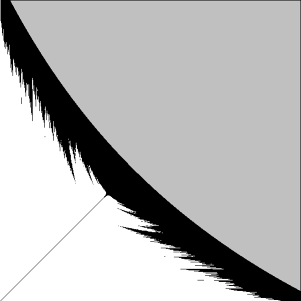
A picture of the set is shown in Figure 1 (which also appears in [9]). It is created by a
program of Christoph Bandt, similar to the one used in [1] to
draw the set . The set
is shaded grey. The algorithm rigorously checks that a point is outside and paints it “white.” The points that are not declared to be “white” after a
certain number of iterations are declared to be in and painted “black.”
Thus the figure should be viewed as an “outward approximation” for .
However, this is not completely accurate; for instance, the apparent
disconnected pieces of are a computing artifact, as we show below.
Another remark is that the computation is very time-consuming near
the diagonal, so the picture is not accurate there.
Figure 1. Connectedness locus for the family of self-affine sets
Next we recall for completeness the results on the set obtained in [9].
Denote
for . We see that the set has an “antenna”
, defined in [9] as the connected component of
containing . In fact, we can consider the set of points on the diagonal which are limit points of . By definition, this
set consists of those for which there exist with real zeros such that . By compactness of it follows that there exists with a double zero at , that is, . Conversely, a point , where
is a double zero of some power series , is in the closure of if has infinitely many coefficients not equal to , since we can
then make an arbitrarily small negative perturbation of staying in , which will result in a pair of real zeros close to .
(Here we use the fact that is necessarily a local minimum of . It cannot be triple zero, since the smallest triple zero of is
at least by [3]; see more about this in the next section.)
It follows from [9] that is disconnected, and it is conjectured to have infinitely many connected components.
The “tip” of the antenna, that is, such that is maximal, is found in [9, Cor.2.10] with
high accuracy: .
Another interesting question concerns the topological structure of . By analogy with the Bandt’s conjecture from [1], we expect
that is contained in the closure of the set of its interior points. It is not obvious even that there exist interior points in the
nontrivial part of , where . However, in [9] it was shown
that a small, but explicitly given, disk around is contained in .
2. Statement of results
There is another method, which does not involve much computing,
to show that certain regions are disjoint from
. It is based on the idea
that it is much easier to estimate zeros
of power series with “convex” restrictions on the coefficients and
uses so-called -functions, first introduced in [10]. We will
also need their generalizations from [3].
Definition 2.1.
A power series is called an
-function if there exist integers such that are any real numbers for
, and
Moreover, we require that has exactly coefficient sign changes. (It is clear from the assumptions on that the number of
sign changes is at most , however, it could potentially be less, if for some we have .)
A -function will be called a -function, and a -function
will be called a -function.
Let
Further, consider
and
By definition, .
For a power series with bounded real coefficients, let denote its positive zeros ordered by magnitude
and counted with multiplicity (for convenience we let if
there are fewer than positive zeros).
In [3] it is proved that for any , the smallest
-th order zero of a power series in is
algebraic, and the corresponding power series is a -function.
In particular, is the positive
zero of .
Proposition 2.2.
(a) The function
is well-defined on . It is continuous,
decreasing, and satisfies
(b) For every we have
(c) For every there exists a unique function in which vanishes at and .
Moreover, it is a
-function
(2.1)
such that . Moreover, and .
The following table contains some values of the function
(rounded-off in such a way that the actual values are slightly
larger):
.51
.52
.53
.54
.55
.56
.57
.58
.59
.862
.831
.811
.79
.77
.755
.742
.728
.716
.6
.61
.62
.63
.64
.703
.691
.68
.67
.658
Note that the -function is in if and only if . Thus, we get a countable set of points which belong to
. It turns out that the set has “cusp corners” at these points, as we show in our first main theorem.
This property distinguishes from the set , which has spiral points and no corners with
interior angle less than (conjecturally, none at all), see [14].
Theorem 2.3.
Suppose that and is such that there is a unique function which vanishes at
and , and moreover, all the coefficients of are eventually and .
Then is a
“tip of a corner” of the set , with zero interior angle.
More precisely, there exist and positive constants and ,
such that
where . In fact, we can take
In particular, these conditions are satisfied if
is a -function, i.e. for some
and .
Remarks. 1. Note that all the points described in the theorem are algebraic, since the function is rational over .
The first “tips of the corners” to which the theorem applies, for an appropriate -function, are as follows (given with 5-6 digit accuracy):
, which is a pair of zeros of (incidentally, the reciprocals of this pair are the golden ratio and the 4th Pisot number);
, which is a pair of zeros of ;
, which is a pair of zeros of ;
, which is a pair of zeros of ;
, which is a pair of zeros of .
2. The “cusp corners” obtained from -functions are only the
“most outward” cusp corners of . There are many others visible in Figures 1 and 2, which are probably
pairs of zeros of power series
with all but finitely many coefficients equal to , as in Theorem 2.3.
For instance, it appears that there is a corner at (with the second zero again the reciprocal of the 4th Pisot number), which is
a pair of zeros of . In order to prove this rigorously, one only needs to check that is the unique function in with this pair of zeros, but we haven’t done this.
Figure 2. The set , with several prominent “cusp corners”
Our second main result is concerned with connectedness properties of the set .
Let
Recall that is the “trivial” part of . .
Theorem 2.4.
The set is locally connected. Moreover,
there is no connected component of that is disjoint from .
We were not able to prove the connectedness of the entire set , but conjecture that this is the case.
The next proposition shows that the last theorem is non-vacuous,
in fact, contains a substantial portion
of the set . In particular, the set is connected near the “cusp corners” from Theorem 2.3.
Let
Clearly, . Recall that denotes
the smallest triple
zero of a power series in ; in [3] it is shown that
is a zero of a polynomial with integer
coefficients of degree 12.
Proposition 2.5.
(a) The function
is well-defined on . It is continuous,
decreasing, and satisfies
(b) For every we have
(c) For every there exists a unique
-function
(2.2)
such that .
The following table contains some values of the function
(rounded-off in such a way that the actual values of are slightly
larger):
.53
.55
.57
.59
.61
.63
.65
.67
.69
.71
.7278
.877
.85
.832
.815
.799
.785
.771
.759
.747
.736
.7278
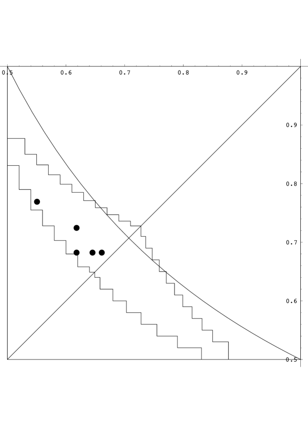
Figure 3.
Propositions 2.2 and 2.5 are
illustrated in Figure 3, which shows the
region obtained from the tables. For in the region below
the lower broken line, the corresponding self-affine
set is totally disconnected. Theorem 2.4 implies that the
part of between the broken lines and outside is locally connected and there are
no components of entirely contained between the broken lines and
the diagonal. We also show several points which are known to belong to
(these are some of the “cusp corners” from Theorem 2.3).
Another application of the bounds on the set
comes from the paper by P. Shmerkin [8]. Following [8, Def. 4.10], we say that is a region of
-transversality if for all there is such that but . It is clear is a region of -transversality. It is proved in [8] that
for Lebesgue-a.e. with the self-affine attractor has Hausdorff dimension
, and if is a region of -transversality contained in , then
has zero Hausdorff measure in its dimension for Lebesgue-a.e. .
3. Proofs
Proof of Proposition 2.2.
Consider the family of -functions
with and , given by (2.1),
and equip it with a total order as follows:
Obviously,
The set is a normal family of analytic functions in the
unit disk; therefore, it is compact in the uniform topology on any compact
subset of . We can also indentify with the
infinite product equipped with the product topology.
Observe that is
a continuous function from to for all .
It is strictly decreasing in the order defined above, and moreover,
By [10] and [3], there is a -function
having a double zero at , with .
It is easy to see that every has exactly two
distinct positive zeros.
Indeed, has at least two positive zeros since ,
, and . On the other hand, the derivative
has only
one coefficient sign change, so it has at most one positive zero
by the Decartes Rule of Signs,
hence has at most two positive zeros.
Clearly, the zeros (when they exist) continuously depend on .
Claim 1.For every there exists a
-function such that .
Indeed, , and for sufficiently large we have
, since .
By continuity, there exist and such that , and
of course, .
Since , there is another zero .
The claim is proved.
Claim 2.We have , and is the unique
function in with zeros at and .
Indeed, suppose
is such that and .
Consider . Then
is a power series with at most one coefficient sign change and .
It follows that is the only positive zero of . The first nonzero
coefficient of is positive, so it is positive for small positive .
It follows that for all , hence
for all . So, for all , , and the claim
is proved.
The claims show that the function is well-defined on .
The remaining statements of part (a) are now easy to derive. In fact, one can obtain sharp asymptotics for as and
, but we do not pursue this.
(b) This statement is immediate from the definition of .
(c) The formula for the “optimal” function and its uniqueness are already
proved.
The statement about the derivative of is also clear: as already mentioned,
has only one sign change and its zero (which the minimum of ) must lie in . ∎
The table of values is obtained from Claims 1 and 2 above. See Appendix for details.
Proof of Theorem 2.3.
Suppose that are such that
. Consider functions (maybe non-unique)
such that
. Since is compact, there is
a subsequence of converging to some , with
. By the assumption of uniqueness of such a function, we have .
Since convergence in is coefficientwise, it follows that for
any there is such that agrees with
in the first terms for all .
This already implies
that is a “corner” with interior angle at most .
Indeed, if agrees with
in the first terms, where is the last term of with a coefficient different from , then has only non-negative coefficients
and hence for all . Since for
we obtain that the zeros of must satisfy
.
For the more delicate estimate we need the following lemma:
Lemma 3.1.
Suppose that are such that and are zeros
of , as in the statement of Theorem 2.3, and let , where is a power series with
coefficients . Then for sufficiently large, has zeros and satisfying
Recall that and by assumption.
First we deduce the theorem, assuming the lemma.
The argument at the beginning of the proof shows that for any there exists such that for all (where ),
if is such that , then
agrees with in the first coefficients. (Note that implies there does indeed exist such that
.)
Let be such that has only coefficients equal to starting from . Let be so small that .
Then
for some power series with coefficients and we obtain from Lemma 3.1:
Let . Note that , so
Thus we have that
Now, and , whence
as desired. The claim that the conditions on are satisfied whenever is a -function is immediate from definitions and Proposition 2.2. ∎
Proof of Lemma 3.1.
This is standard, but we provide the argument for completeness. We will only prove the estimate for , since the one for is obtained
in exactly the same way. We will need an easy inequality:
(3.1)
Recall that and , so to the right of
. Thus, it is clear that for large there will be a zero of in a small neighborhood
. Since the claim is local, we can assume that for some (independent of ,
e.g. we can take ).
We have . Recall that , and we want to make sure that
. By Taylor’s formula,
Thus we can choose sufficiently large, so that
.
Next,
which is also less than for sufficiently large.
Then , whence
, and so we have
from (3.2):
as desired. ∎
Proof of Theorem 2.4.
This proof is a modification of the argument by Bandt [1, Section 11], which is, in turn, based on [5].
Let
and
consider the quotient space
(3.3)
with induced topology. Denote by the point corresponding to the
contracted boundary.
Recall that is the set of all power series of the
form , with .
We can identify with the space equipped
with the product topology. Observe that this topology coincides with the
topology of uniform convergence on compact subsets of the unit disk.
Claim 1. is relatively closed in .
ndeed, let and
. Then
there exist with and
. This means that there exist
such that
(if is equal to or this is understood as
having the corresponding zero of multiplicity 2).
By compactness, without loss of generality, we
can assume that and . Then
and
(again using our convention concerning double zeros). Thus , and Claim 1 is proved.
We will also need the following fact (see [3] and [8, Th. 2.4]): if and are (some) complex roots of in the unit disk, counted with multiplicity, then
Taking , we obtain
(3.4)
Let be the function defined as follows:
If is such that and
, then
; otherwise, .
Claim 2. is continuous.
Indeed, if ,
then has simple zeros at and , hence a small perturbation
of will result in a small perturbation of these zeros.
Suppose that .
We need to show that if is
a small perturbation of , then is close to .
We have the following possibilities:
(a) has no positive zeros;
(b) has one simple positive zero;
(c) but
;
(d) ;
(e) ;
(f) , that is, has a triple zero.
It is not hard to see that for any there exists such
that if the distance from to in is less than ,
then every zero of in is -close to a
zero of . Another general fact is useful: for a small perturbation of a real-analytic function, new real zeros cannot appear; zeros can only
dissappear (i.e. become non-real).
In cases (a) and (b), either has the same
property, hence , or new zeros appear near 1, which
could result in with near 1, that is,
is close to in the topology of .
In the case (c), a small perturbation will have
or , which is
close to ,
hence close to in the topology of . Suppose that case (d) holds. If the double zero at doesn’t dissappear, then
we either still have a double zero for , or two real zeros close to each other. In the former case we have , and in the
latter case is close to the diagonal, that is, close to in the topology of . If, on the other hand, the double zero dissappears (becomes non-real) and
, then , which is close to
where are zeros of and
. However, in the latter case we have by (3.4), hence
and so is still close to . If (e) or (f) holds, we have
a similar argument: assuming , this point is either close to one
in , or close to the diagonal, or close to , in view of (3.4). This concludes the proof of Claim 2.
Now we essentially repeat the argument from [5]. For a finite
word in the alphabet let
Denote by the word of length obtained by adding the
symbol to .
Let . We have
.
Observe that these three functions have the same set of zeros in ,
hence they are mapped into the same point by . It follows that
for an arbitrary .
This property is called recursive connectedness in [5].
It is proved in [5] (and quite easy to see) that this property
implies that is connected and locally connected in .
Note that
where is the natural
projection associated with the quotient map. (We know that
since, for instance,
there are power series in with no positive zeros.)
This immediately implies the statement of the theorem. ∎
Proof of Proposition 2.5.
By [9, Cor. 2.5.], for any there exists such that and has at least three
zeros in (for example, we may take the zeros of to be with multiplicity one, and with multiplicity two). Thus the set in the definition of the function
is non-empty; it has a minimum by compactness of the class .
The statement (b) is immediate from the definitions.
The remaining statements of (a) will easily follow from part (c).
Its proof is divided into several lemmas.
Lemma 3.2.
Suppose that is a -function such that
and for all . Then there is no such that , unless , and
is a triple zero of .
Proof. Suppose that violates the
assertion of the lemma.
Let . By the definition of a -function, we have
where and are polynomials and is a power series,
all three
with non-negative coefficients, such that the highest power in
is less than the lowest power in . Thus, and
have at most two coefficient sign changes each.
Since is the third zero of and , we have . (Indeed, otherwise is negative in a left neighborhood of , but
on an interval where a real-analytic function changes its sign it must have an odd number of zeros, counting with multiplicities.)
Thus, . Observe that there must be a zero
of between the
first and second zeros of (if these two zeros of coincide, that is,
it is a double zero, which is equal to ). We have ,
hence , and
. By the Decartes Rule of Signs, can have at most
two positive zeros. There has to be a zero of in .
There also have to be another zero of in , since , , and .
Thus, has exactly two
coefficient sign changes, hence .
But then increases sufficiently close to zero, whence must have
at least two zeros in . This is a contradiction. ∎
Lemma 3.3.
.
Proof. Suppose there exists such that
.
It is proved in [3] that there is a -function
such that . (In fact, and .) Consider the function
This is a -function, though not necessarily in , since the -coefficient may exceed 1 in absolute value.
We have for , hence
for all and by definition.
We claim that for all . Indeed, has
two coefficient sign changes, hence at most two positive zeros.
We know that is negative near zero, , , and
is negative sufficiently close to 1. It follows that has a zero
in , so it does not vanish in , implying the claim.
Thus, is a
-function satisfying the assumptions of Lemma 3.2
for , so the existence of is a contradiction. ∎
Lemma 3.3 implies that for
.
Fix .
Recall that is well-defined, which means that there exists
a function such that . Such
a function will be called “optimal” (for a given ).
Lemma 3.4.
An optimal function for has a double zero at
, that is, .
Proof.
Suppose . Since and is the third
positive zero of a real analytic function, is strictly decreasing
in a neighborhood of . By Decartes’ Rule of Signs, has at least
three coefficient sign changes. Therefore, we can find integers
such that and , where is the coefficient of in .
Consider
Then for sufficiently small .
Moreover, and for .
Thus, for sufficiently small , the function
has a zero close to which is less than . We claim that
this zero is , which contradicts .
Indeed, if the first two positive zeros of are distinct (and they are
smaller than ), this property will persist for . If is
a double zero, then has a second zero close to .
This proves the claim, and the lemma follows. ∎
Lemma 3.5.
The optimal function for is unique; it is a
-function for some
and .
Proof.
Let
be optimal, and suppose that it is not a -function
(see (2.2)).
Let
be minimal such that . Then choose
minimal such that (note that exists since
must have at least three coefficient sign changes).
If is not a -function, then we can find such that
. Let be such that
satisfies . (This is a linear system of equations with determinant ,
so there is a unique solution.)
Notice that and , since there must be two coefficient sign changes in
. Clearly, is a simple zero for , and it is a double zero for
by Lemma 3.4. Thus, there exist such that
for near . Consider
Then for sufficiently small . Observe that
by construction. Recall that , and , hence . We
can make sure that is so small that
. On the other hand,
provided that . Then has a zero in which
implies that . Since , we have
, so is optimal for (as well as ).
This contradicts Lemma 3.5 since is not a double zero
of . It remains to verify that the optimal function is unique.
Assuming that we have two distinct optimal functions, we take their difference,
which has at most two
coefficient sign changes, since both are -functions.
This leads to a contradiction since the difference has at least three
positive zeros.
This concludes the proof of the lemma and of the claim (c) in Proposition 2.5. The remaining statements of the proposition
follow easily. ∎
4. Appendix: how to compute the functions and
We first explain how the function was computed, using Mathematica.
Consider the -function , where .
First, we fix . The algorithm takes as an input. Then, is determined so that . We must check that , so that is indeed a member of . Next, we find the second root of using the FindRoot command with an appropriate starting point. We choose the starting point to guarantee that we find rather than (FindRoot uses Newton’s method to find the root of a function. It will find the root closest to the starting point. Recall the shape of the -function . We must choose a starting point to the right of the minimum of to guarantee that Mathematica finds rather than . We know our choice of starting point works as long as the output of FindRoot is not equal to our input ).
Now, as was seen in [10, 3],
there is a -function having a double zero at . Therefore we begin by fixing .
Consider the -function . We solve for to ensure that
and obtain
.
We find that 0.8 works as a starting point for FindRoot.
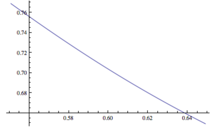
Using NSolve, we find that for , approximately. However, recall that . Thus we are only interested in looking at . Figure 4 shows a plot of for .
Figure 4. from
Now, note that when , . Thus at , the coefficient of is . Thus this is a “switching point,” that is, at this point, switches to a -function with . This is one of the points we are interested in, because it will be in the set .
Next we consider the -function , so that . We solve for so that is indeed a root of , and find .
We again check the range for which , and find that the inequality holds for .
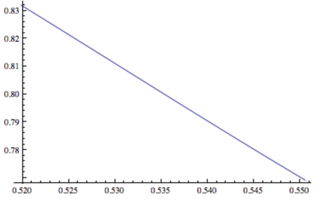
Figure 5. from
Figure 5 shows a plot of for .
Note that , so that at becomes a -function with . Thus we continue similarly by setting . Let , and solve for so that to obtain
.
Using NSolve, we find that for .
We may continue in this manner in order to obtain for . Note, however, that the process does not terminate.
Now we explain how the function may be computed.
Recall that , where .
Consider the -function
where .
Recall that we would like to find such that . Since we have two unknowns and , for this algorithm we will start with and obtain and such that , and use FindRoot to find such that .
In [3] it was proved that there is a -function H= such that .
Thus we begin by considering the function . Then we let .
Note that .
We solve the system of equations
for and and find that and .
In this case, we need to have both and .
We find that for , (note that ) and for (where ). So, the first coeffcient that “switches” is at , when .
Next we use FindRoot to find . So this algorithm takes as an input and outputs , so this is effectively .
Next, we use our “switching point.” We let and and solve for and so that . We find that and .
Again we check for which we have and and continue in this way.
Acknowledgment.
This paper was started in 2003, but took a long time complete. Its preliminary drafts are cited in [8, 9]. Thanks to Pablo Shmerkin for helpful discussions and fruitful collaboration on [9]. I am grateful to Christoph Bandt for his help with the computer program
(which he specially wrote on my request), without which this paper would have been impossible. Thanks also to Allison
Beckwith who helped with the Appendix, as part of her Master’s project at the University of Washington Department
of Mathematics during 2011-2012.
References
[1] C. Bandt, On the Mandelbrot set for pairs of linear maps,
Nonlinearity15 (2002), 1127–1147.
[2] M. F. Barnsley, Fractals Everywhere, Academic Press,
1988.
[3] F. Beaucoup, P. Borwein, D. W. Boyd, and
C. Pinner, Multiple roots of power series, J. London Math. Soc.(2)57 (1998), 135–147.
[4] M. F. Barnsley and A. N. Harrington, A Mandelbrot set
for pairs of linear maps, Physica15D (1985), 421–432.
[5] T. Bousch, Connexité locale et par chemins hölderiens
pour les systèmes itérés de fonctions, Preprint, 1993,
http://topo.math.u-psud.fr/~bousch
[6] I. Eroğlu, S Rohde, and B. Solomyak,
Quasisymmetric conjugacy between quadratic dynamics and iterated function systems, Ergodic Theory Dynam. Systems30 (2010), no. 6, 1665–1684.
[7] M. Hata, On the structure of self-similar sets,
Japan. J. Appl. Math.2 (1985), 381–414.
[9] P. Shmerkin and B. Solomyak,
Zeros of power series and connectedness loci for self-affine sets, Experiment. Math.15 (2006), no. 4, 499–511.
[10] B. Solomyak, On the random series
(an Erdős problem),
Annals of Math.142 (1995), 611–625.
[11] B. Solomyak,
Measure and dimension of some fractal families,
Math. Proc. Cambridge Phil. Soc.124, no. 3 (1998), 531–546.
[12] B. Solomyak,
On the ‘Mandelbrot set’ for pairs of linear maps: asymptotic self-similarity, Nonlinearity18 (2005), no. 5, 1927–1943.
[13] B Solomyak and H. Xu,
On the ‘Mandelbrot set’ for a pair of linear
maps and complex Bernoulli convolutions,
Nonlinearity16 (2003), no. 5, 1733–1749.
[14] B. Solomyak,
“Mandelbrot set” for a pair of linear maps: the local geometry, Analysis in Theory and Applications20:2 (2004), 149–157.