Energy density matrix formalism for interacting quantum systems: a quantum Monte Carlo study

Abstract

We develop an energy density matrix that parallels the one-body reduced density matrix (1RDM) for many-body quantum systems. Just as the density matrix gives access to the number density and occupation numbers, the energy density matrix yields the energy density and orbital occupation energies. The eigenvectors of the matrix provide a natural orbital partitioning of the energy density while the eigenvalues comprise a single particle energy spectrum obeying a total energy sum rule. For mean-field systems the energy density matrix recovers the exact spectrum. When correlation becomes important, the occupation energies resemble quasiparticle energies in some respects. We explore the occupation energy spectrum for the finite 3D homogeneous electron gas in the metallic regime and an isolated oxygen atom with ground state quantum Monte Carlo techniques implemented in the QMCPACK simulation code. The occupation energy spectrum for the homogeneous electron gas can be described by an effective mass below the Fermi level. Above the Fermi level evanescent behavior in the occupation energies is observed in similar fashion to the occupation numbers of the 1RDM. A direct comparison with total energy differences shows a quantitative connection between the occupation energies and electron addition and removal energies for the electron gas. For the oxygen atom, the association between the ground state occupation energies and particle addition and removal energies becomes only qualitative. The energy density matrix provides a new avenue for describing energetics with quantum Monte Carlo methods which have traditionally been limited to total energies.

The single particle or mean field picture has been widely used to explain the physics of quantum-mechanical systems. Both qualitative and quantitative models based on the notion that individual electrons occupy distinct energy levels are indispensible in the analysis of bonding, transport, and optical phenomena, among many others.martin04 Yet if interactions are fully taken into account, the picture becomes more complicated with correlation tangling together the previously independent states into a single many-body state. Despite the added complexity, it is known that some single particle features are preserved in the presence of correlation. From the success of Fermi liquid theory,pines66 for example, we know that the low-lying excitations in many-body systems with weak effective interactions can behave like collections of nearly independent quasiparticles. Even far from the Fermi level, any many-body quantum state contains a strong analogy to the single particle picture: the natural orbitals and occupation numbers that are made accessible from the one body reduced density matrix (1RDM).lowdin55 Whether a complementary representation of energy levels exists for these single particle states is less clear.

Quantum Monte Carlofoulkes01 methods that deal directly with the complexity of the many body problem, usually provide energetic information at the level of a single number: the total energy. While this is useful, a more detailed picture of energetics could broaden the interpretive power of such methods. Recent workkrogel13 has shown that the total energy of a many-body quantum system can be partitioned across space into an energy density. This hints that an underlying orbital representation of energetics might be accessible through the energy density.

In this work we expand the concept of energy density to include non-locality, arriving at an energy density matrix. The one body reduced energy density matrix (1REDM) provides energetic information complementary to the established 1RDM. In particular, diagonalization of the 1REDM provides a set of natural energy orbitals and single particle occupation energies. Just as in the mean field picture, the combination of these single particle energies reduces to the total energy of the system. Analogous to the 1RDM, the spectrum of the energy density matrix represents a compact partitioning of the total energy (rather than the particle number) across states, consisting of strongly occupied states below the Fermi energy and weakly occupied states above it. It will be shown that the occupation energies share a close relationship with particle addition and removal energies.

The remainder of the paper is organized as follows. In section I we derive the non-local energy density matrix from the energy density following the example of the 1RDM. The total energy sum rule is proved and a Schrödinger-like equation is derived for the natural energy orbitals and occupation energies of the matrix. Section II is devoted to an empirical investigation of the properties of the occupation energy spectrum via ground state continuum quantum Monte Carlo techniques. In section II.1 the occupation energy spectrum is calculated for a series of finite homogeneous electron gases (HEG’s) at the same density. The behavior of the spectrum under removal or spin flip of a single electron at constant volume for a small HEG is analyzed in section II.2. Section II.3 explores the occupation spectrum of the open shell oxygen atom in its ground state. A summary of our results is contained in section III. Details regarding the quantum Monte Carlo evaluation of the energy density matrix, as implemented in QMCPACK,kim12 can be found in appendix A.

I Derivation and properties of the energy density matrix

The one body reduced energy density matrix is closely related to the 1RDM. For systems with exchange symmetry, the 1RDM, $n_{1}(r,r^{\prime})$, is obtained by integrating out all particle coordinates but one from the $N$-body density matrix, $\rho_{N}(R,R^{\prime})$ and normalizing to the number of particles, $N$:

$$n_{1}(r,r^{\prime})=N\int dR_{1}\rho_{N}(r,R_{1},r^{\prime},R_{1}).$$ (1)

Both here and in the formulae that follow, $R=[r_{1},...,r_{N}]$ denotes all particle coordinates, while $R_{i}=[r_{1},...,r_{i-1},r_{i+1},...,r_{N}]$ is the full set with particle $i$ removed. Spin indices have been suppressed for simplicity of discussion. Rewriting Eq. 1 more symmetrically and introducing the partial trace over $N-1$ particles, $Tr_{R_{i}}(*)\equiv\int dR_{i}\langle R_{i}\rvert*\lvert R_{i}\rangle$, we arrive at the more compact matrix form,

$$\hat{n}_{1}=\sum_{i}Tr_{R_{i}}\hat{\rho}_{N}$$ (2)

Since the $N$ particle density matrix is normalized to one ($Tr\hat{\rho}_{N}=1$), the particle sum rule quickly follows:

$$Tr\hat{n}_{1}=\sum_{i}Tr\hat{\rho}_{N}=\sum_{i}1=N.$$ (3)

The density can be obtained either from the diagonal part of the 1RDM or from the expectation value of the density operator, $\hat{n}(r)=\sum_{i}\delta(r-r_{i})$:

$$n(r)=Tr(\hat{n}(r)\hat{\rho}_{N})=\langle r\rvert\hat{n}_{1}\lvert r\rangle$$ (4)

With this connection in mind, we are now prepared to identify the energy density matrix from the evaluation of the energy density.

The energy density operator reflects the partitioning of energy among particles. Here we take a perspective consistent with the notion of a mean-field, i.e., that electrons carry an energy reflecting an average of the surrounding particles (this differs from the definition in reference krogel13, where an additive partitioning of energy among all particle species was sought). The energy carried by or belonging to electron $i$ can be defined as

$$\hat{h}_{i}=\hat{t}_{i}+\hat{v}^{ext}(r_{i})+\frac{1}{2}\sum_{j\neq i}\hat{v}^{ee}(r_{i},r_{j}),$$ (5)

which is symmetric under particle exchange. Here $\hat{t}_{i}=-\tfrac{1}{2}\nabla^{2}_{i}$ is the kinetic energy of particle $i$, $\hat{v}^{ext}(r)$ represents the external potential, including local Coulomb or fully non-local pseudopotential ions, and $\hat{v}^{ee}(r_{i},r_{j})=1/\lvert r_{i}-r_{j}\rvert$ is the Coulomb potential between electrons. The energy density operator simply tracks the energy located at point $r$ in real space and reduces to the Hamiltonian when integrated:

$$\hat{\mathcal{E}}(r)=\sum_{i}\delta(r-r_{i})\hat{h}_{i},$$ (6)

$$\int dr\hat{\mathcal{E}}(r)=\sum_{i}\hat{h}_{i}=\hat{H}.$$ (7)

Anticipating that the energy density matrix (1REDM) $\hat{\mathcal{E}}_{1}$ can be identified in a similar fashion to the 1RDM

$$\mathcal{E}(r)=Tr(\hat{\mathcal{E}}(r)\hat{\rho}_{N})=\langle r\rvert\hat{\mathcal{E}}_{1}\lvert r\rangle$$ (8)

we evaluate the expectation value of the energy density

$$\mathcal{E}(r) =Tr(\sum_{i}\delta(r-r_{i})\hat{h}_{i}\hat{\rho}_{N})$$

$$=\int dR\langle R\rvert\sum_{i}\delta(r-r_{i})\hat{h}_{i}\hat{\rho}_{N}\lvert R\rangle$$

$$=\sum_{i}\int dR_{i}\langle r,R_{i}\rvert\hat{h}_{i}\hat{\rho}_{N}\lvert r,R_{i}\rangle$$

$$=\langle r\rvert\sum_{i}Tr_{R_{i}}\hat{h}_{i}\hat{\rho}_{N}\lvert r\rangle.$$ (9)

We immediately see that the 1REDM can be defined as

$$\hat{\mathcal{E}}_{1}=\sum_{i}Tr_{R_{i}}\hat{h}_{i}\hat{\rho}_{N}.$$ (10)

quantity	formula	sum rule
number density	$\begin{aligned} n(r)=\langle r\rvert\hat{n}_{1}\lvert r\rangle\end{aligned}$	$\begin{aligned} \int drn(r)=N\end{aligned}$
energy density	$\begin{aligned} \mathcal{E}(r)=\langle r\rvert\hat{\mathcal{E}}_{1}\lvert r\rangle\end{aligned}$	$\begin{aligned} \int dr\mathcal{E}(r)=E\end{aligned}$
number in $\phi_{\ell}$	$\begin{aligned} n_{\phi_{\ell}}=\langle\phi_{\ell}\rvert\hat{n}_{1}\lvert\phi_{\ell}\rangle\end{aligned}$	$\begin{aligned} \sum_{\ell}n_{\phi_{\ell}}=N\end{aligned}$
energy in $\phi_{\ell}$	$\begin{aligned} \mathcal{E}_{\phi_{\ell}}=\langle\phi_{\ell}\rvert\hat{\mathcal{E}}_{1}\lvert\phi_{\ell}\rangle\end{aligned}$	$\begin{aligned} \sum_{\ell}\mathcal{E}_{\phi_{\ell}}=E\end{aligned}$
number spectrum	$\begin{aligned} \hat{n}_{1}\lvert\eta_{\ell}\rangle=n_{\ell}\lvert\eta_{\ell}\rangle\end{aligned}$	$\begin{aligned} \sum_{\ell}n_{\ell}=N\end{aligned}$
energy spectrum	$\begin{aligned} \hat{\mathcal{E}}_{1}\lvert\xi_{\ell}\rangle=\mathcal{E}_{\ell}\lvert\xi_{\ell}\rangle\end{aligned}$	$\begin{aligned} \sum_{\ell}\mathcal{E}_{\ell}=E\end{aligned}$

Table 1: Comparison of related quantities derived from the 1-body reduced density $\hat{n}_{1}$ and energy density $\hat{\mathcal{E}}_{1}$ matrices, including the density, occupation of an arbitary orbital $\phi_{\ell}$ (assumed to be part of a complete set), and eigenvalue/occupation spectrum. $N$ is the total number of particles and $E$ is the total energy.

From the definition of the 1REDM several properties quickly become apparent. Since many of these properties are directly analogous to those of the 1RDM we present a side-by-side comparison in table 1. Perhaps the most interesting of these is that the energy density matrix provides access to a single particle energy spectrum embedded in the many body state. Minimizing the energy $\mathcal{E}_{\xi}=\langle\xi\rvert\hat{\mathcal{E}}_{1}\lvert\xi\rangle$ contained in an arbitrary state $\lvert\xi\rangle$ results in a set of natural energy orbitals $\lvert\xi_{\ell}\rangle$ and occupation energies $\mathcal{E}_{\ell}$

$$\hat{\mathcal{E}}_{1}\lvert\xi_{\ell}\rangle=\mathcal{E}_{\ell}\lvert\xi_{\ell}\rangle.$$ (11)

It can be shown that certain quantum numbers describing the many-body state (e.g. crystal momentum) are transferred to the natural energy orbitals.

For a mean-field system, the occupation energy spectrum is identical to the spectrum of the 1-body Hamiltonian. This can be demonstrated by calculating the explicit representation of the energy density matrix for the mean field system. In this case, the $N$-body Hamiltonian is given by the sum of identical 1-body operators $\hat{H}^{MF}=\sum_{i}\hat{h}^{MF}(r_{i})$ and the wavefunction is a Slater determinantslater29 of the occupied orbitals, denoted $\Psi^{MF}$, with the orbitals obeying the single particle Schrödingerschrodinger26 equation $\hat{h}^{MF}\lvert\phi_{n}^{MF}\rangle=\mathcal{E}_{n}\lvert\phi_{n}^{MF}\rangle$. The energy density matrix can be obtained in real space following a process similar to the derivation of the Slater-Condonslater29 ; condon30 rules for one-body operators.

$$\mathcal{E}_{1}(r,r^{\prime}) =\sum_{i}\int dR_{i}\hat{h}^{MF}_{r}\Psi^{MF}(r,R_{i})\Psi^{MF*}(r^{\prime},R_{i})$$

$$=\sum_{i}\hat{h}^{MF}(r)\phi^{MF}_{i}(r)\phi^{MF*}_{i}(r^{\prime})$$

$$=\sum_{i}\mathcal{E}^{MF}_{i}\phi^{MF}_{i}(r)\phi^{MF*}_{i}(r^{\prime})$$ (12)

This is just the spectral representation of $\hat{h}^{MF}$ and so the eigenvalues and eigenvectors of the energy density matrix are $\{\mathcal{E}^{MF}_{n}\}$ and $\{\lvert\phi^{MF}_{n}\rangle\}$, respectively. Since $\{\lvert\phi^{MF}_{n}\rangle\}$ are also the natural orbitals in this case ($\lvert\eta^{MF}_{n}\rangle=\lvert\phi^{MF}_{n}\rangle$), any deviation between $\{\lvert\eta_{n}\rangle\}$ and $\{\lvert\xi_{n}\rangle\}$ for an interacting system is a direct indication of the strength of correlation effects beyond what can be captured by an effective mean field. For many systems that are not strongly correlated, the natural orbitals and the natural energy orbitals are expected to be similar.

A characteristic property of a mean-field system is that the total energy is just the sum of the single particle energies $E^{MF}=\sum_{i=1}^{N}\mathcal{E}^{MF}_{i}$. This property is preserved in the spectrum of the energy density matrix even for interacting systems because it obeys the following total energy sum rule

$$Tr\hat{\mathcal{E}}_{1}=Tr\sum_{i}\hat{h}_{i}\hat{\rho}_{N}=Tr(\hat{H}\hat{\rho}_{N})=E$$ (13)

which is similar to the particle sum rule of the 1RDM $Tr\hat{n}_{1}=N$. The spectral representation of the sum rule is similar to the mean field form

$$\sum_{\ell=1}^{\infty}\mathcal{E}_{\ell}=E.$$ (14)

It is expected that states with vanishing occupation number will also make vanishing contributions to the total energy, provided the occupation spectrum is bounded from below and non-oscillatory.

Unlike the mean-field case, the total energy for an interacting system is not a linear functional of the occupation numbers. Factoring the energy density matrix in terms of one- and two-body contributions gives

$$\hat{\mathcal{E}}=(\hat{t}+\hat{v}^{ext})\hat{n}_{1}+\hat{v}^{ee}_{1}.$$ (15)

Here $\hat{t}$ and $\hat{v}^{ext}$ are the one-body kinetic and external potential operators given in Eq. 5, $\hat{n}_{1}$ is the 1RDM, and $\hat{v}^{ee}_{1}$ is the one-body reduced electron-electron interaction matrix given by

$$\hat{v}^{ee}_{1}=\sum_{i}Tr_{R_{i}}\bigg{(}\frac{1}{2}\sum_{j\neq i}\hat{v}^{ee}(r_{i},r_{j})\hat{\rho}_{N}\bigg{)}.$$ (16)

Upon expanding the total energy in the basis of natural orbitals

$$E =\sum_{\ell}\langle\eta_{\ell}\rvert\hat{\mathcal{E}}_{1}\lvert\eta_{\ell}\rangle$$

$$=\sum_{\ell}\left[n_{\ell}\langle\eta_{\ell}\rvert\hat{t}+\hat{v}^{ext}\lvert\eta_{\ell}\rangle+\langle\eta_{\ell}\rvert\hat{v}^{ee}_{1}\lvert\eta_{\ell}\rangle\right]$$ (17)

we see that the one body terms contribute linearly in occupation number while the two body interaction term involving $\hat{v}_{1}^{ee}$ will in general contain higher order contributions. This is consistent with expectations based on Landau’s theory of quantum fluidslandau57 where terms up to quadratic order in occupation number are retained in the total energy functional.

The natural energy orbitals obey a Schrödinger-like integro-differential equation, which can be obtained by combining expressions 11 and 15 and projecting into real space:

$$\left[-\frac{1}{2}\nabla^{2}_{r}+v^{ext}(r)\right]\int dr^{\prime}n_{1}(r,r^{\prime}) \xi_{\ell}(r^{\prime})$$

$$+\int dr^{\prime}v^{ee}_{1}(r,r^{\prime}) \xi_{\ell}(r^{\prime})=\mathcal{E}_{\ell}\xi_{\ell}(r)$$ (18)

The form of this equation resembles the quasi-particle equation arising in $GW$ theory.hedin65 The resemblance in form becomes stronger in the case of weak correlation ($\xi_{\ell}(r)\approx\eta_{\ell}(r)$)

$$\left[-\frac{1}{2}\nabla^{2}_{r}+v^{ext}(r)\right] \xi_{\ell}(r)$$

$$+\int dr^{\prime}\frac{v^{ee}_{1}(r,r^{\prime})}{n_{\ell}} \xi_{\ell}(r^{\prime})=\frac{\mathcal{E}_{\ell}}{n_{\ell}}\xi_{\ell}(r)$$ (19)

with $v^{ee}_{1}(r,r^{\prime})/n_{\ell}$ and $\mathcal{E}_{\ell}/n_{\ell}$ filling the roles of self-energy and quasi-particle energy level, respectively. It should be stressed at this point that the eigenvalues of Eq. I formally correspond to particle removal energies in the weakly-interacting limit, in contrast to $GW$. Another important distinction to keep in mind is that Eqs. I and I provide a single particle energy spectrum measured within a particular many body state, $\hat{\rho}_{N}$. The full single particle spectrum is obtained by combining measurements over all states in the many-body spectrum.

Defining the energy of a particular level as

$$\bar{\mathcal{E}}_{\ell}=\frac{\mathcal{E}_{\ell}}{n_{\xi_{\ell}}}=\frac{\langle\xi_{\ell}\rvert\hat{\mathcal{E}}_{1}\lvert\xi_{\ell}\rangle}{\langle\xi_{\ell}\rvert\hat{n}_{1}\lvert\xi_{\ell}\rangle}$$ (20)

is sensible because $\bar{\mathcal{E}}_{\ell}$ shifts rigidly with a constant shift in the external potential while $\mathcal{E}_{\ell}$ does not (to see this, note from Eq. 15 that $\hat{\mathcal{E}}_{1}\rightarrow\hat{\mathcal{E}}_{1}+v_{c}\hat{n}_{1}$ when $\hat{v}^{ext}\rightarrow\hat{v}^{ext}+v_{c}$). Since the number of electrons in the level is $n_{\xi_{\ell}}=\langle\xi_{\ell}\rvert\hat{n}_{1}\lvert\xi_{\ell}\rangle$, it is consistent that the energy in the level is the product of the energy level and its occupation, or $n_{\xi_{\ell}}\bar{\mathcal{E}}_{\ell}=\mathcal{E}_{\ell}$, which is the portion of the total energy attributed to $\lvert\xi_{\ell}\rangle$.

By distinguishing an energy level from the amount of energy occupied in that level, we can further partition the energy among spin species where spin interactions are small enough to be neglected. In this case a well-defined spin state can be formed by assigning each electron to have an up or down spin and the 1RDM, along with its corresponding occupation numbers, can be factored into up and down components. The occupation energies for spin up or down electrons can then be defined as

$$\mathcal{E}^{\uparrow/\downarrow}_{\ell}=n^{\uparrow/\downarrow}_{\xi_{\ell}}\bar{\mathcal{E}}_{\ell}=\frac{n^{\uparrow/\downarrow}_{\xi_{\ell}}}{n_{\xi_{\ell}}^{\uparrow}+n_{\xi_{\ell}}^{\downarrow}}\mathcal{E}_{\ell}.$$ (21)

This relation has been used in all following sections to obtain spin-resolved occupation energies.

II Exploration of the occupation energy spectrum

In the preceeding analysis both rigorous connections and analogies to mean-field behavior have been made, but a more empirical investigation of the remaining properties of the occupation energy spectrum is clearly warranted. In the following two sections we analyze the occupation spectrum for the fully interacting 3D homogeneous electron gas (HEG), first for the ground state over a range of system sizes and then for excited states of a small system. Study of the excited state systems probes the relationship between the occupation energies and single particle addition and removal for the HEG. Following the analysis of the HEG we explore the partitioning of the energy among core and valence states for the open shell ground state of the oxygen atom.

II.1 Ground state occupation energies of the homogeneous electron gas

The homogeneous electron gas is an ideal test case to explore the properties of the occupation energy spectrum. We calculate the energy density matrix and its spectrum for a series of finite systems with 14, 38, 54, 66, 114, 162, and 186 electrons in cubic periodic cells $(L^{3}=V)$. These electron counts correspond to closed shell fillings with inversion symmetry in momentum space. The electron density is determined by the parameter $r_{s}\equiv(3V/4\pi N)^{1/3}=3.0$, which is in the metallic regime of the HEG.

The ground state of the non-interacting system is a Slater determinant of plane waves, $e^{ikr}$, with each 3-dimensional component $k_{d}$ of $k$ satisfying $k_{d}=2\pi n_{d}/L$. In this case, the exact occupation spectrum must follow the dispersion relation $\mathcal{E}_{k}=\hbar^{2}k^{2}/2m_{e}$ below the Fermi momentum ($k<k_{F}$) and vanish above it since the unoccupied states do not contribute to the total energy. Since the occupation energies are known for the non-interacting case, it serves as a useful test of our implementation of energy density matrix estimators in QMCPACK (see appendix A for implementation details). The occupation energies obtained from diffusion Monte Carlogrimm71 ; anderson75 (DMC) calculations are shown in the top panel of figure 1. The solid shapes correspond to energy density matrix (1REDM) eigenvalues, $\mathcal{E}_{k}$, for the various finite systems. The dashed black curve shows the exact dispersion for an infinite system which is strictly positive because the Hamiltonian is comprised of kinetic energy only. The energy spectrum follows the expected parabolic dispersion curve for all system sizes, confirming that the energy density matrix estimators have been implemented correctly in QMCPACK.

Figure 1: Occupation energies for the 3D homogeneous electron gas at $r_{s}=3$ from diffusion Monte Carlo calculations vs. crystal momentum (solid shapes). The top panel contains results for the non-interacting system with the black dashed line representing the expected dispersion of $\hbar^{2}k^{2}/2m_{e}$. Results for the interacting system are in the lower panel. The dashed green line is a $\hbar^{2}k^{2}/2m^{*}$ fit with $m^{*}=0.84m_{e}$ and the black dashed line is the standard dispersion shifted to match at $k=0$. $N$ is the number of electrons in each finite simulation.

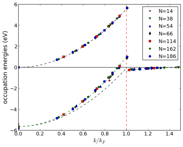
In the presence of electron-electron interactions the natural orbitals and natural energy orbitals are constrained by symmetry to remain plane waves but the ground state wavefunction and hence its 1RDM and 1REDM become more complex. Fully interacting occupation energies from the 1REDM are shown in the lower panel of figure 1. The dominant effect of interactions is a constant energy shift of just under $6~{}eV$ for the strongly occupied states below the Fermi level, arising partly from the uniform positive background present in jellium. The dashed black line in the lower panel of figure 1 is the non-interacting spectrum shifted to match at $k=0$. Interactions only partly average out with the electron-electron repulsion raising the occupation energies at larger $k$ by up to $1~{}eV$. Since the dispersion remains approximately parabolic, this effect can be summed up in terms of an effective mass, $m^{*}$. A dispersion with $m^{*}=0.84m_{e}$ provides a good fit to the interacting occupation energies as shown by the dashed green curve. This suggests a possible relationship between quasiparticle energies and the occupation energies since the quasiparticles are known to acquire an effective mass. Previous quasiparticle calculations based on self-consistent $GW$rietschel83 and related approacheskrakovsky96 find an effective mass near $0.9m_{e}$. Effective masses for the two dimensional HEG obtained with Quantum Monte Carlo total energy differences are also generally smaller than $GW$ results.kwon94 ; kwon96 ; drummond13

Figure 2: Similar to figure 1 but for occupation numbers of the 1RDM. Simulations of interacting systems deviate from one(zero) below(above) $k_{F}$. The dashed green lines are exponential fits of the deviation from ideal behavior about $k_{F}$. For comparison, the solid black curves are polynomial fits to the DMC data of Ortiz and Balloneortiz94 ; ortiz97 .

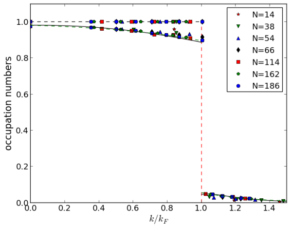
Another known effect of interactions is that the occupation numbers of the 1RDM become finite above $k_{F}$ while the discontinuity at the Fermi surface is reduced. Figure 2 shows the DMC eigenvalues of the 1RDM vs. particle count from our calculations. The occupation numbers above the Fermi surface decrease exponentially with increasing momentum. Despite the rapid decay, fully $7\%$ of the particle weight resides above the Fermi surface. This effect is also visible in the occupation energy spectrum above $k_{F}$ in figure 1. Similar to the occupation numbers, the occupation energies also decrease exponentially with $k$ above the Fermi surface and cumulatively account for $10\%$ of the total energy. We expect this behavior to generalize to other systems with strongly occupied states below the Fermi level (which carry most of the energy) being accompanied by a large number of weakly occupied states providing evanescent energy contributions. The fraction of the total energy residing above the Fermi level, as obtained from the energy density matrix, can be viewed as a measure of correlation. With this metric, the correlation energy of any mean field system is precisely zero.

II.2 Occupation energies for selected excitations of a 14 electron HEG

In order to explore the relationship between the occupation energies obtained from the 1REDM and electron addition and removal energies, we have performed additional DMC calculations on the 14 electron system. The first of these is a direct charge removal from the outermost filled spin down shell performed at constant volume. The second is a spin flip excitation where an electron in the outermost spin down shell is promoted to a new unfilled spin up shell. In both cases we compare total energy differences relative to the unperturbed 14 electron state with results from the active occupation energies. The active space is defined as the set of natural energy orbitals that experienced a significant change in the spin-resolved occupation number between the initial and final states. Eigenstates that did not significantly vary in occupation number are further separated into core states (with occupation number closer to one) and virtual states (with occupation number closer to zero). Although the comparison is made here for a small system for simplicity and convenience, the conclusions drawn from these results should not qualitatively depend on system size.

Figure 3: DMC occupation energies for a 13 electron HEG vs. state index (solid shapes) resolved by spin with spin up in blue and spin down in red. State 1 corresponds to $k=0$ and states 2 through 7 belong to the same shell $k\in\{\pm\Delta k\hat{x},\pm\Delta k\hat{y},\pm\Delta k\hat{z}\}$. A single electron has been removed from the spin down channel of state 7.

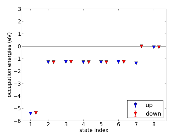
Spin resolved occupation energies (see Eq. 21) for the system with a single electron removed are shown in figure 3. Spin up(down) states are represented by the blue(red) triangles. The $k=0$ state (state 1) is lowest in energy and all 6 states in the second shell ($\lvert k\rvert=\Delta k$ are degenerate. The electron removal is clearly visible with the previously degenerate 7th spin down state displaying an occupation energy near zero. Only this state (state 7) has experienced a significant change in occupation number and so the active space contains this state alone. Since the neighboring spectrum is changed only a small amount, total energy differences will be dominated by the active space as core and virtual contributions to energy differences largely cancel.

Charged systems in periodic boundary conditions experience a shift in the reference potential relative to the neutral statecorsetti2011 ; komsa2012 . The relative difference in occupation energy of the first and second shells for the neutral and charged systems is identical to within error bars and so the potential shift can safely be obtained by aligning the core levels. This is effected by applying a constant potential energy shift of $-0.11~{}eV$ to the charged system. Calculating the potential shift from core occupation energies might also prove useful to QMC studies of charged defect systems which are generally restricted to small supercells.

Figure 4: DMC occupation energies for a 14 electron HEG spin flip excitation vs. state index (solid shapes) resolved by spin with spin up in blue and spin down in red. A single electron has been removed from the spin down channel of state 7 and added to the spin up channel of state 8, which belongs to the third shell, $k=2\Delta k\hat{x}$.

Having taken the alignment potential into account, a meaningful comparison of total energy differences and changes in the active occupation energies can be made. The charge removal energy obtained from DMC total energy differences is $\Delta E_{tot}=E_{tot}^{7^{\uparrow}6^{\downarrow}}-E_{tot}^{7^{\uparrow}7^{\downarrow}}=1.43(2)~{}eV$. For comparison the change in occupation energy over the active space is $\Delta E_{active}=\mathcal{E}_{7^{\downarrow}}^{7^{\uparrow}6^{\downarrow}}-\mathcal{E}_{7^{\downarrow}}^{7^{\uparrow}7^{\downarrow}}=1.27(1)~{}eV$. The occupation energy of the active state in the neutral system accounts for about $90\%$ of the ionization energy ($-\mathcal{E}_{7^{\downarrow}}^{7^{\uparrow}7^{\downarrow}}=1.28(1)~{}eV$). The other $10\%$ is scattered across the core and virtual spaces as the result of correlation, which is consistent with the fraction of total energy residing above the Fermi level we have already witnessed in the ground state. Although some of the energy is dispersed across the state space, the large concentration of energy residing in a single state indicates that the occupation energies of the 1REDM are closely related to particle addition and removal energies for this system.

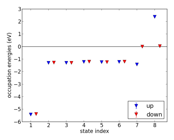
This relationship is also confirmed in the case of a spin flip excitation. Occupation energies for a 14 electron HEG with 8 up and 6 down electrons can be found in figure 4. The spectrum is similar to the charge removal case for states 7 and below since the spin flip consists of removing an electron from the spin down channel of state 7 and then adding it to the spin up channel of state 8, which resides on a higher energy shell. The active space is comprised of these two states. Since the filled shell and spin-flipped systems have the same charge the constant background potentials are already aligned and the spectra can be compared directly. The energy required to flip the spin is $\Delta E_{tot}=E_{tot}^{8^{\uparrow}6^{\downarrow}}-E_{tot}^{7^{\uparrow}7^{\downarrow}}=3.98(2)~{}eV$ according to DMC total energies and $\Delta E_{active}=\mathcal{E}_{8^{\uparrow}}^{8^{\uparrow}6^{\downarrow}}+\mathcal{E}_{7^{\downarrow}}^{8^{\uparrow}6^{\downarrow}}-\mathcal{E}_{8^{\uparrow}}^{7^{\uparrow}7^{\downarrow}}-\mathcal{E}_{7^{\downarrow}}^{7^{\uparrow}7^{\downarrow}}=3.71(3)~{}eV$ according to the active occupation energies. The fraction of energy contained in the active space for the spin flip is similar to the charge removal case.

II.3 Occupation energies of the oxygen atom

Figure 5: DMC occupation energies for the ground state of a neutral oxygen atom with 5 up and 3 down electrons (solid triangles). Experimental binding energies (negative of ionization potential) of the first through the eighth electron in oxygen are shown as dashed horizontal lines as a comparative energy scale.

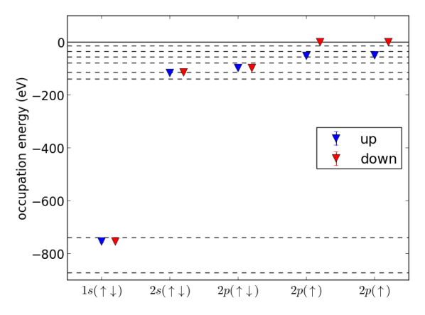
Diffusion Monte Carlo occupation energies obtained with QMCPACK for an all-electron oxygen atom in its electronic ground state are shown in figure 5. In this case, the energy density matrix has been expanded in a basis of 46 orbitals obtained from a Hartree-Fockhartree28 ; fock30 ; roothaan51 calculation performed with the GAMESSschmidt93 ; gordon05 simulation package. The spin state of the atom is clearly reflected in the occupation spectrum with three electron pairs occupying $1s$, $2s$, and $2p$ states along with two unpaired spin down (blue triangles) electrons in the outermost valence states. The spin up (red triangles) partner orbitals of the unpaired electrons are unoccupied as indicated by their near zero occupation energies. The negatives of experimental ionization energies (i.e. the binding energies of single electrons for successive ionizations) are shown in dashed black lines to give a comparative energy scale. This comparison is useful because these binding energies and the occupation energies must add up to the total energy ($E_{tot}^{exp}=-2043.81~{}eV$, $E_{tot}^{DMC}=-2042.29(4)~{}eV$). The $1s$ electrons are very deeply bound in the ground state with occupation energies of $-753(4)~{}eV$. This value resides fairly close to the experimental binding energy of $-739.29~{}eV$ for the first $1s$ electron of the $O^{6+}$ ion. This demonstrates that the occupation spectrum has remained bounded in a physical way despite the strong inhomogeneity of the nucleus.

Moving up the spectrum, we see that the ground state $2s$ electron occupation energies are similarly close to the experimental binding energy of the first $2s$ electron of the $O^{4+}$ ion and so the large gap between $1s$ and $2s$ states is represented well. Out in the $2p$ valence states we see a rather different distribution of energy in the ground state relative to energies imparted to electrons upon ionization. The occupation energies of the $2p$ states are rather deep. This implies that electronic relaxation effects will be quite pronounced for the occupation energies of the 1REDM, with many occupation energies changing during ionization. It is not fully clear why the occupation energies resemble electron removal energies rather well for the homogeneous electron gas and poorly for inhomogeneous oxygen. It is true that the occupation energies resulting from the energy density matrix are not formally guaranteed to obey Koopman’s theorem except in the weakly-interacting limit. In this respect the correspondence between the occupation energies and particle addition/removal energies will depend on the system being studied. The occupation energies in figure 5 are on the same scale as the experimental binding energies and so they do remain related, although not as closely, to electron removal energies for this system.

III Summary

We have introduced a new observable for many-body quantum systems, the energy density matrix, analogous to the well established one body reduced density matrix. The natural orbitals of the two matrices are similar, with the 1RDM providing particle number information in the form of occupation numbers and the 1REDM providing a complementary description of energetics in the form of occupation energies. We have also argued that the evanescent portion of the occupation energy spectrum and the deviations between the two sets of orbitals are a signal of strong correlation effects. It has been shown that the occupation energies obey a total energy sum rule, similar to both the mean field case and the Landau total energy functional for quantum fluids. We have also demonstrated that the eigenstates of the energy density matrix obey a Schrödinger-like equation that is similar in form to the standard quasiparticle equation. The resulting occupation energies for the homogeneous electron gas in the metallic regime resemble quasiparticle energies, in the sense that the spectrum can be described in terms of an effective mass. The occupation energies also approximate electron addition and removal energies for this system as demonstrated by direct comparison with total energy differences for simple charge and spin excitations. In the inhomogeneous case, studied here for a single oxygen atom, the occupation spectrum of the ground state remains bounded from below and reproduces some features of the experimental electron binding energies. The overall quantitative agreement is rather poorer than for HEG, however, showing that the correspondence is not fully general. With further development the energy density matrix may provide a useful tool to describe single particle energetics with quantum Monte Carlo methods which have traditionally been limited to total energies.

Appendix A Quantum Monte Carlo evaluation

This section details the practical evaluation of the energy density matrix within standard ground-state continuum quantum Monte Carlo methods such as variationalmcmillan65 (VMC) or diffusion Monte Carlo (DMC). The formal details and recent applications of these methods have been covered elsewherefoulkes01 ; bajdich09 ; needs10 ; kolorenc11 ; wagner14 and we refer the interested reader to these sources to obtain a full account. These methods are treated here in the abstract, but sufficient detail is retained to unambigously sample the energy density matrix in a real simulation code.

In DMC one measures observables relative to the mixed $N$-body density matrix

$$\hat{\rho}^{DMC}_{N}=\lvert\Psi\rangle\langle\Psi_{0}\rvert.$$ (22)

Here $\Psi$ represents the analytically defined trial wavefunction and $\Psi_{0}$ is the fixed node/phase approximation to the ground state as produced by the diffusion and branching process of Monte Carlo walkers. VMC results are obtained by the substitution $\Psi_{0}\rightarrow\Psi$. The expectation value of observable $A$ is obtained in the usual way:

$$\langle A\rangle =Tr\hat{A}\hat{\rho}^{DMC}_{N}=\langle\Psi_{0}\rvert\hat{A}\lvert\Psi\rangle$$

$$=\int dR\Psi^{*}_{0}(R)\Psi(R)\frac{A\Psi(R)}{\Psi(R)}.$$ (23)

The DMC process explicitly draws configuration space samples $\{R\}$ from the mixed probability distribution $\Psi^{*}_{0}(R)\Psi(R)$.

An efficient and compact representation of the energy density matrix can be obtained by projection onto a suitably chosen single particle basis $\{\phi_{i}\}$. In the case of the HEG these are plane waves, while for systems composed of atoms it is convenient to use orbitals from Hartree-Fock or DFT calculations. In the low energy subset of the basis, a finite and discrete approximation to the energy density matrix ($\mathcal{E}_{1ij}$) is obtained.

$$\mathcal{E}_{1ij} =\langle\phi_{i}\rvert\hat{\mathcal{E}}_{1}\lvert\phi_{j}\rangle$$

$$=\langle\phi_{i}\rvert\sum_{n}Tr_{R_{n}}\hat{h}_{n}\hat{\rho}^{DMC}_{N}\lvert\phi_{j}\rangle$$

$$=\sum_{n}\int dR_{n}dr_{n}dr^{\prime}_{n}\phi_{i}^{*}(r_{n}^{\prime})h(r_{n}^{\prime},R_{n})$$

$$\qquad\qquad\times\Psi(r_{n}^{\prime},R_{n})\Psi_{0}^{*}(r_{n},R_{n})\phi_{j}(r_{n})$$

$$=\int dR\Psi_{0}^{*}(R)\Psi(R)\sum_{n}\phi_{j}(r_{n})$$

$$\times\int dr^{\prime}_{n}\frac{\Psi(r_{n}^{\prime},R_{n})}{\Psi(r_{n},R_{n})}\phi_{i}^{*}(r_{n}^{\prime})\frac{h(r_{n}^{\prime},R_{n})\Psi(r_{n}^{\prime},R_{n})}{\Psi(r_{n}^{\prime},R_{n})}$$ (24)

For systems involving non-local pseudopotentials, the factor $h(r_{n}^{\prime},R_{n})\Psi(r_{n}^{\prime},R_{n})$ is replaced with $\int d\bar{r}_{n}h(r_{n}^{\prime},\bar{r}_{n},R_{n})\Psi(\bar{r}_{n},R_{n})$, where $\bar{r}_{n}$ represents the additional non-local coordinate.

Equation A is a valid way to measure $\hat{\mathcal{E}}_{1}$, but it is inefficient since the additional integral over $r_{n}^{\prime}$ involves a re-evaluation of the Hamiltonian components $h(r_{n}^{\prime},R_{n})$ at each integration point. A more efficient form can be obtained without a loss of accuracy. Upon switching the primed coordinates $r_{n}\leftrightarrow r_{n}^{\prime}$ and rearranging, we obtain

$$\mathcal{E}_{1ij} =\sum_{n}\int dRdr_{n}^{\prime}\Psi^{*}(R)\Psi(R)\frac{\Psi_{0}^{*}(r_{n}^{\prime},R_{n})}{\Psi(r_{n},R_{n})}\phi_{i}^{*}(r_{n})$$

$$\quad\times\phi_{j}(r_{n}^{\prime})\frac{h(r_{n},R_{n})\Psi(R)}{\Psi(R)}$$

$$\approx\sum_{n}\int dRdr_{n}^{\prime}\Psi_{0}^{*}(R)\Psi(R)\frac{\Psi^{*}(r_{n}^{\prime},R_{n})}{\Psi^{*}(r_{n},R_{n})}\phi_{i}^{*}(r_{n})$$

$$\quad\times\phi_{j}(r_{n}^{\prime})\frac{h(r_{n},R_{n})\Psi(R)}{\Psi(R)}$$

$$=\int dR\Psi_{0}^{*}(R)\Psi(R)\sum_{n}\frac{h(r_{n},R_{n})\Psi(R)}{\Psi(R)}\phi_{i}^{*}(r_{n})$$

$$\quad\times\int dr_{n}^{\prime}\frac{\Psi^{*}(r_{n}^{\prime},R_{n})}{\Psi^{*}(r_{n},R_{n})}\phi_{j}(r_{n}^{\prime})$$ (25)

This representation is more efficient because the quantities involving $h(r_{n},R_{n})$ have already been computed at each Monte Carlo configuration $R$. In this way the energy density matrix can be computed at no additional cost over the 1RDM. The additional integral over $r_{n}^{\prime}$ can be evaluated approximately as a Riemann sum over a randomly shifted uniform grid, as is done in this work, or from a set of points sampled from the single particle density. Reusing the same set of points for each value of $n$ additionally reduces the number of required orbital evaluations by a factor of $N$, but the relatively expensive wavefunction ratios must still be computed for each $n$.

We will now show that the approximation in Eq. A does not affect the accuracy of the computed energy density matrix. For simplicity of discussion we will actually consider the 1RDM since the approximation above affects the sampling of each matrix in the same fashion. The 1RDM in DMC is

$$n_{1}(r,r^{\prime})=\sum_{n}\int dR_{n}\Psi(r,R_{n})\Psi_{0}^{*}(r^{\prime},R_{n}).$$ (26)

Considering instead the 1RDM arising from the adjoint of $\hat{\rho}^{DMC}_{N}$

$$n_{1}(r,r^{\prime})^{\dagger} =\sum_{n}\int dR_{n}\Psi_{0}(r,R_{n})\Psi^{*}(r^{\prime},R_{n})$$

$$=\sum_{n}\int dR_{n}\Psi(r,R_{n})\Psi_{0}^{*}(r^{\prime},R_{n})$$

$$\qquad\times\frac{\Psi_{0}(r,R_{n})}{\Psi(r,R_{n})}\frac{\Psi^{*}(r^{\prime},R_{n})}{\Psi_{0}^{*}(r^{\prime},R_{n})}$$ (27)

we see that it differs from the original by the kernel

$$K^{T}(r,r^{\prime},R_{n})=\frac{\Psi_{0}(r,R_{n})}{\Psi(r,R_{n})}\frac{\Psi^{*}(r^{\prime},R_{n})}{\Psi_{0}^{*}(r^{\prime},R_{n})}.$$ (28)

The approximation in equation A is equivalent to introducing the kernel

$$K^{A}(r,r^{\prime},R_{n})=\frac{\Psi_{0}^{*}(r,R_{n})}{\Psi^{*}(r,R_{n})}\frac{\Psi^{*}(r^{\prime},R_{n})}{\Psi_{0}^{*}(r^{\prime},R_{n})}.$$ (29)

For VMC $\Psi_{0}\rightarrow\Psi$ and $K^{A}_{VMC}=K^{T}_{VMC}=1$. For fixed-node (FN) and released-node (RN) DMC the wavefunction is real ($\Psi_{0}^{*}=\Psi_{0}$, $\Psi^{*}=\Psi$) and

$$K^{A}_{FN}=K^{T}_{FN}=\frac{\Psi_{0}(r,R_{n})}{\Psi(r,R_{n})}\frac{\Psi(r^{\prime},R_{n})}{\Psi_{0}(r^{\prime},R_{n})}.$$ (30)

Fixed-phase (FP) DMC gives a similar result since the trial wavefunction and its projection are contrained to share the same phase ($\Psi_{0}=\lvert\Psi_{0}\rvert e^{i\phi}$, $\Psi=\lvert\Psi\rvert e^{i\phi}$) which yields

$$K^{A}_{FP}=K^{T}_{FP}=\frac{\lvert\Psi_{0}(r,R_{n})\rvert}{\lvert\Psi(r,R_{n})\rvert}\frac{\lvert\Psi(r^{\prime},R_{n})\rvert}{\lvert\Psi_{0}(r^{\prime},R_{n})\rvert}.$$ (31)

In all of these cases the 1RDM and the 1REDM are effectively being measured from $\hat{\rho}_{N}^{\dagger}$ which has the same level of accuracy as $\hat{\rho}_{N}$. Additionally, the sum rules summarized in table 1 are all preserved since $K^{A}(r,r,R_{n})=1$.

References

- (1) R. M. Martin, Electronic Structure: Basic Theory and Practical Methods (Cambridge Univ. Press, Cambridge, 2004).
- (2) D. Pines and P. Nozières, The Theory of Quantum Liquids. Vol. 1: Normal Fermi Liquids (W. A. Benjamin, Inc., New York, 1966).
- (3) P.-O. Löwdin, Phys. Rev. 97, 1474 (1955).
- (4) W. M. C. Foulkes, L. Mitas, R. J. Needs, and G. Rajagopal, Rev. Mod. Phys. 73, 33 (2001).
- (5) J. T. Krogel, M. Yu, J. Kim, and D. M. Ceperley, Phys. Rev. B 88, 035137 (2013).
- (6) J. Kim et al., J. Phys. Conf. Ser. 402, 012008 (2012).
- (7) J. C. Slater, Phys. Rev. 34, 1293 (1929).
- (8) E. Schrödinger, Phys. Rev. 28, 1049 (1926).
- (9) E. U. Condon, Phys. Rev. 36, 1121 (1930).
- (10) L. Landau, Soviet Physics Jetp-Ussr 3, 920 (1957).
- (11) L. Hedin, Phys. Rev. 139, A796 (1965).
- (12) R. Grimm and R. Storer, J. Comput. Phys. 7, 134 (1971).
- (13) J. B. Anderson, J. Chem. Phys. 63, 1499 (1975).
- (14) G. Ortiz and P. Ballone, Phys. Rev. B 50, 1391 (1994).
- (15) G. Ortiz and P. Ballone, Phys. Rev. B 56, 9970 (1997).
- (16) H. Rietschel and L. J. Sham, Phys. Rev. B 28, 5100 (1983).
- (17) A. Krakovsky and J. K. Percus, Phys. Rev. B 53, 7352 (1996).
- (18) Y. Kwon, D. M. Ceperley, and R. M. Martin, Phys. Rev. B 50, 1684 (1994).
- (19) Y. Kwon, D. M. Ceperley, and R. M. Martin, Phys. Rev. B 53, 7376 (1996).
- (20) N. D. Drummond and R. J. Needs, Phys. Rev. B 87, 045131 (2013).
- (21) F. Corsetti and A. A. Mostofi, Phys. Rev. B 84, 035209 (2011).
- (22) H.-P. Komsa, T. T. Rantala, and A. Pasquarello, Phys. Rev. B 86, 045112 (2012).
- (23) D. R. Hartree, in Mathematical Proceedings of the Cambridge Philosophical Society (Cambridge Univ. Press, Cambridge, 1928), No. 01, pp. 89–110.
- (24) V. Fock, Zeitschrift für Physik 61, 126 (1930).
- (25) C. C. J. Roothaan, Rev. Mod. Phys. 23, 69 (1951).
- (26) M. W. Schmidt et al., Journal of Computational Chemistry 14, 1347 (1993).
- (27) M. S. Gordon and M. W. Schmidt, in Theory and Applications of Computational Chemistry: the first forty years, edited by C. E. Dykstra, G. Frenking, K. S. Kim, and G. E. Scuseria (Elsevier, Amsterdam, 2005), pp. 1167–1189.
- (28) W. McMillan, Phys. Rev. 138, A442 (1965).
- (29) M. Bajdich and L. Mitas, Acta Physica Slovaca. Reviews and Tutorials 59, 81 (2009).
- (30) R. J. Needs, M. D. Towler, N. D. Drummond, and P. L. Ríos, Journal of Physics: Condensed Matter 22, 023201 (2010).
- (31) J. Kolorenc and L. Mitas, Reports on Progress in Physics 74, 026502 (2011).
- (32) L. K. Wagner, International Journal of Quantum Chemistry 114, 94 (2014).