Controlling observables in time-dependent quantum transport

Abstract

The theory of time-dependent quantum transport addresses the question: How do electrons flow through a junction under the influence of an external perturbation as time goes by? In this paper, we invert this question and search for a time-dependent bias such that the system behaves in a desired way. This can, for example, be an observable that is forced to follow a certain pattern or the minimization of an objective function which depends on the observables. Our system of choice consists of quantum dots coupled to normal or superconducting leads. We present results for junctions with normal leads where the current, the density or a molecular vibration is optimized to follow a given target pattern. For junctions with two superconducting leads, where the Josephson effect triggers the current to oscillate, we show how to suppress the Josephson oscillations by suitably tailoring the bias. In a second example involving superconductivity, we consider a Y shaped junction with two quantum dots coupled to one superconducting and two normal leads. This device is used as a Cooper pair splitter to create entangled electrons on the two quantum dots. We maximize the splitting efficiency with the help of an optimized bias.

I Introduction

Molecular quantum transport is a fast growing research field. The ultimate goal is to produce electronic devices using single molecules as their building blocks Aviram and Ratner (1974); Cuniberti et al. (2005); Di Ventra (2008); Cuevas and Scheer (2010). The prospective improvements regarding operational speed as well as storage capacity are expected to be enormous if the miniaturization of transistors can be taken to the scale of single molecules.

In the past, the main objective was to measure and/or calculate the current-voltage characteristics of the molecular junction. On the theory side, calculations were usually done within the Landauer-Büttiker approach. In recent years, interest has shifted more and more towards time-resolved studies. Such studies allow one to address questions like: How long does it take until the steady state is reached? Can we shorten or lengthen this time span? Does a steady state always exist, and if so, is it unique? To answer this kind of questions by calculations, explicitly time-dependent approaches are necessary, such as time-dependent density functional theory Runge and Gross (1984); Baer et al. (2004); Burke et al. (2005); Kurth et al. (2005); Yuen-Zhou et al. (2009); Di Ventra and D’Agosta (2007); Appel and Di Ventra (2009, 2011), the Kadanoff-Baym equations Stefanucci and van Leeuwen (2013); Myöhänen et al. (2009, 2010); Knap et al. (2011), multi-configuration time-dependent Hartree-Fock Zanghellini et al. (2004); Wang and Thoss (2009, 2013); Albrecht et al. (2012), Quantum Monte-Carlo Mühlbacher and Rabani (2008), time-dependent tight binding Wang et al. (2011); Zhang et al. (2013); Oppenländer et al. (2013), or the hierarchy equation of motion approach Jin et al. (2008); Zheng et al. (2008a, b).

In all those approaches the reaction of the molecular junction to a given external perturbation, i.e. a bias or a gate voltage is calculated. In this article, we want to take a step beyond this point and control the current or other observables of the junction. This means we have to address the inverse question: Which perturbation leads to a desired reaction of the system? To answer this question, optimal control theory provides a suitable framework. This research field was pioneered by the work of Pontryagin Pontryagin et al. (1962) and Bellman Bellman (1957) who paved the way for numerous applications. Initially, optimal control theory was mainly used to solve problems of classical mechanics. Later, it found applications in many other research fields including quantum mechanics. Peirce et al. (1988); Shenghua et al. (1988); Kosloff et al. (1989)

A particularly interesting field goes under the heading of “femto-chemistry” where chemical reactions are influenced with femto-second laser pulses such that a specific reaction gets suppressed or enhanced. Assion et al. (1998); Hartke et al. (1989); Elghobashi et al. (2003); Elghobashi and Gonzalez (2004) A successful experimental application is the selective bond dissociation of molecules. Levis et al. (2001) Other applications of optimal control theory in the quantum world include the control of the electron flow in a quantum ring Räsänen et al. (2007), the accelerated cooling of molecular vibrations Reich and Koch (2013), the control of the entanglement of electrons in quantum wells Räsänen et al. (2012), the optimization of quantum revival Räsänen and Heller (2013), the control of ionization Castro et al. (2009); Räsänen and Madsen (2012) or the selection of transitions between molecular states Jakubetz et al. (1990).

Kleinekathöfer and coworkers combined optimal control theory with the master equation approach for quantum transport and demonstrated the control of various observables in junctions with normal leads Li et al. (2007); Amin et al. (2009); Li and Kleinekathöfer (2010). We take a different approach to the same problem by propagating wave functions. For the time propagation, we employ an algorithm proposed by Stefanucci et al. Stefanucci et al. (2010). This allows us to treat not only normal (N) but also superconducting (S) leads.

The paper is organized as follows: In section II, we explain the model Hamiltonian that we employ to describe the molecular junctions. In section III, we formulate the optimization problem for tailoring the bias such that a chosen observable follows s predefined pattern as best as possible. Various results are presented in section IV. Finally, in section V, we focus on a specific example, a Y shaped junction consisting of two quantum dots coupled to one superconducting and two normal leads. This device is used as a Cooper-pair splitter, for which we maximize the splitting efficiency. In the final section VI, we draw our conclusions.

II Model

Our model system consists of a quantum dot (QD) connected to two semi-infinite, non-interacting one dimensional leads (L and R), which are described by a tight binding Hamiltonian. Later, in section V, we will add a third lead (labeled S) and a second quantum dot. The corresponding changes in the Hamiltonian will then be stated in that section but the overall approach and the structure of the equations stays the same.

The Hamiltonian for the junction with two leads and a single quantum dot reads

$$\hat{H}(t) =\hat{H}_{\textnormal{QD}}+\sum_{\alpha\in\{\textnormal{L},\textnormal{R}\}}\hat{H}_{\alpha}+\sum_{\alpha\in\{\textnormal{L},\textnormal{R}\}}\hat{H}_{T,\alpha}(t)$$ (1)

with

$$\hat{H}_{\textnormal{QD}} =\epsilon_{\textnormal{QD}}\sum_{\sigma\in\{\uparrow,\downarrow\}}\hat{d}_{\sigma}^{\dagger}\hat{d}_{\sigma},$$ (2)

$$\hat{H}_{\alpha} =\sum_{k=0}^{\infty}\sum_{\sigma\in\{\uparrow,\downarrow\}}\left(t_{\alpha}\hat{c}_{\alpha k\sigma}^{\dagger}\hat{c}_{\alpha(k+1)\sigma}+H.c.\right),$$ (3)

$$\qquad+\sum_{k=0}^{\infty}\left(\Delta_{\alpha}e^{i\chi_{\alpha}}\hat{c}_{\alpha k\uparrow}^{\dagger}\hat{c}_{\alpha k\downarrow}^{\dagger}+H.c.\right),$$

$$\hat{H}_{T,\alpha}(t) =\sum_{\sigma\in\{\uparrow,\downarrow\}}\left(t_{\alpha,\textnormal{QD}}e^{i\gamma_{\alpha,\textnormal{QD}}(t)}\hat{c}_{\alpha 0\sigma}^{\dagger}\hat{d}_{\sigma}+H.c.\right).$$ (4)

Here $\gamma_{\alpha,\textnormal{QD}}(t)=\int_{0}^{t}\,dt^{\prime}U_{\alpha}(t^{\prime})$ are the Peierls’ phases with the bias $U_{\alpha}(t),\alpha\in\{\textnormal{L},\textnormal{R}\}$. The operator $\hat{c}_{\alpha k\sigma}^{\dagger}$ ($\hat{c}_{\alpha k\sigma}$) creates (annihilates) an electron at site $k\in\mathbb{N}$ in the lead $\alpha\in\{\textnormal{L},\textnormal{R}\}$ with spin $\sigma\in\{\uparrow,\downarrow\}$. The operator $\hat{d}_{\sigma}^{\dagger}$ ($\hat{d}_{\sigma}$) represents the creation (annihilation) of an electron on the quantum dot.

The observables of prime interest, the density $n_{\textnormal{QD}}(t)$ and the current $I_{\alpha,\textnormal{QD}}(t)$, are given by

$$n_{\textnormal{QD}}(t) =\sum_{\sigma\in\{\uparrow,\downarrow\}}\langle\hat{d}_{\sigma}^{\dagger}(t)\hat{d}_{\sigma}(t)\rangle,$$ (5)

$$I_{\alpha,\textnormal{QD}}(t) =2\Im\sum_{\sigma\in\{\uparrow,\downarrow\}}\left(t_{\alpha,\textnormal{QD}}e^{i\gamma_{\alpha,\textnormal{QD}}(t)}\langle\hat{c}_{\alpha 0\sigma}^{\dagger}(t)\hat{d}_{\sigma}(t)\rangle\right).$$ (6)

All parameters in equations (1) - (4) are real and positive. We always work at temperature $T=0$ and in the wide band limit $t_{\alpha,\textnormal{QD}}\ll t_{\alpha}$, where the coupling to the leads is given by $\Gamma=\Gamma_{\textnormal{L}}+\Gamma_{\textnormal{R}},\Gamma_{\alpha}=\frac{2t_{\alpha,\textnormal{QD}}^{2}}{t_{\alpha}},\alpha\in\{\textnormal{L},\textnormal{R}\}$. In this limit, the results only depend on the couplings $\Gamma_{\alpha}$ but not on the hopping elements individually. The superconducting pairing potentials $\Delta_{\alpha}$ can be written as $\Delta_{\alpha}=\xi_{\alpha}\tilde{\Delta}$, which allows a dimensionless representation of the problem by measuring times in units of $\tilde{\Delta}^{-1}$ and energies as well as currents in units of $\tilde{\Delta}$. In the case of normal leads, we set $\xi_{\alpha}=0$, and $\xi_{\alpha}=1$ otherwise. The presence of superconductivity requires the use of the time-dependent Bogoliubov-de Gennes equation

$$i\frac{\,d}{\,dt}\left(\begin{matrix}u_{q}(k,t)\\ v_{q}(k,t)\end{matrix}\right) =\sum_{l}\mathbf{H}_{kl}(t)\left(\begin{matrix}u_{q}(l,t)\\ v_{q}(l,t)\end{matrix}\right),$$ (7)

$$\mathbf{H}_{kl}(t) =\left(\begin{matrix}\mathbf{h}_{kl}(t)&\mathbf{\Delta}_{kl}\\ \mathbf{\Delta}_{kl}^{\dagger}&-\mathbf{h}_{kl}^{\dagger}(t)\end{matrix}\right).$$ (8)

The single-particle wave functions

$$\psi_{q}(k,t)=[u_{q}(k,t),v_{q}(k,t)]^{t}$$ (9)

represent the time-dependent particle- and hole-amplitudes at site $k$. The algorithm for the time propagation of the single particle wave functions $\psi_{q}(k,t)$ as well as the initial state calculation is explained in the work of Stefanucci et al. Stefanucci et al. (2010), which extends the method of Kurth et al. Kurth et al. (2005) to superconducting leads.

III Optimization problem

We start at $t=0$ in the ground state of the junction with $U_{\alpha}(t\leq 0)=0$. The goal is to tailor the bias $U_{\alpha}(t)$ such that the observable of choice $O(t)$ follows a predefined target pattern as best as possible. The corresponding optimization problem reads

$$\min_{U_{\textnormal{L}}(t),U_{\textnormal{R}}(t)}\|O[\Psi](t)-O^{(\textnormal{target})}(t)\|_{2,[0,T]}^{2}\quad\quad$$ (10)

$$\begin{array}[]{rrl}\text{s.t.}&i\partial_{t}\psi_{q}(t)&=\mathbf{H}[U_{\textnormal{L}},U_{\textnormal{R}}](t)\psi_{q}(t),\ t\in[0,T],\\ &\quad\ \psi_{q}(0)&=\psi_{q}^{0}.\end{array}$$ (12)

Here, $\|\cdot\|_{2,[0,T]}$ denotes the $L^{2}$-norm on the time interval $[0,T]$, i.e. the objective function is the following integral:

$$\int_{0}^{T}\,dt|O[\Psi](t)-O^{(\textnormal{target})}(t)|^{2}.$$ (13)

The integral is well-defined since $T$ and the integrand are finite in all examples studied in this work.

Most common is a variational approach to this problem, like the Rabitz approach Zhu et al. (1998) or Krotov’s method Sklarz and Tannor (2002); Palao and Kosloff (2003). Such an approach incorporates the constraints into the objective function using Lagrange multipliers and searches for the roots of the variation of the new objective function. An alternative approach, which we shall adopt in this article, is the direct minimization of the objective function using derivative-free minimization algorithms. This strategy was successfully used in several works Castro et al. (2009); Krieger et al. (2011); Hellgren et al. (2013); Räsänen et al. (2013). In this way, we avoid various difficulties arising from the time propagation algorithm. This approach can be viewed as the computational analogue to the closed-loop learning algorithms employed in experimental optimization Judson and Rabitz (1992).

The basic idea of our numerical approach is to approximate $U_{\alpha}(t)$ by cubic splines with $N+1$ equidistant nodes at $\tau_{k}=\frac{k}{N}T,k\in\{0,\ldots,N\}$. We choose $\frac{\,d}{\,dt}U_{\alpha}(\tau_{0})=\frac{\,d}{\,dt}U_{\alpha}(\tau_{N})=0$ as the boundary conditions for the splines. The dependence of the problem (10) on the bias $U_{\alpha}(t)$ is replaced by

$$U_{\alpha}(t)\to\left[U_{\alpha}(\tau_{0}),\ldots,U_{\alpha}(\tau_{N})\right]\equiv\vec{u}_{\alpha}.$$ (14)

In this way, the spline-interpolated bias $U_{\alpha}(\vec{u}_{\alpha},t)$ becomes a function of $\vec{u}_{\alpha}$. This then yields a normal non-linear optimization problem with the unknown variables $U_{\alpha}(\tau_{k})$. We further impose the condition $U_{\alpha}(\tau_{0})=0$ since the bias has to be continuous and we assume $U_{\alpha}(t<0)=0$. Figure 1 demonstrates this approach.

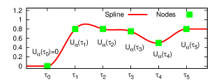
Figure 1: Cubic spline interpolation using six nodes $\tau_{k}$. The optimization algorithm changes the values $U_{\alpha}(\tau_{k}),k\in\{1,\ldots,5\}$. The value $U_{\alpha}(\tau_{0})$ is fixed to zero. The derivatives at both ends are set to zero. The spline does not necessarily take the maximum or minimum value at one of the nodes. In this example, the maximum lies between $\tau_{1}$ and $\tau_{2}$.

Additionally, we add the constraint $U_{\textnormal{L}}(t)=-U_{\textnormal{R}}(t)$ unless otherwise stated, since it reduces the dimensionality of the optimization problem in the numerical implementation by a factor of two. This implies the constraint $\vec{u}_{\textnormal{L}}=-\vec{u}_{\textnormal{R}}$. The resulting non-linear optimization problem is

$$\min_{\vec{u}_{\textnormal{L}},\vec{u}_{\textnormal{R}}\in\mathbb{R}^{N+1}}\|O[\Psi](t)-O^{(\textnormal{target})}(t)\|_{2,[0,T]}^{2}\quad\quad\qquad$$ (15)

$$\begin{array}[]{rcl}\textnormal{s.t.}\quad i\partial_{t}\psi_{q}(t)&=&\mathbf{H}(\vec{u}_{\textnormal{L}},\vec{u}_{\textnormal{R}},t)\psi_{q}(t),\ t\in[0,T],\\ \psi_{q}(0)&=&\psi_{q}^{0},\\ \vec{u}_{\textnormal{L}}&=&-\vec{u}_{\textnormal{R}},\\ U_{\alpha}(\vec{u}_{\alpha},\tau_{0})&=&0,\quad\alpha\in\{\textnormal{L},\textnormal{R}\}.\end{array}$$ (20)

The single particle wave functions $\psi_{q}(t)$ in the problem (15) are only auxiliary variables. Hence, the time-dependent Bogoliubov-de Gennes equation can be removed from the constraint equations for the numerical implementation. The objective function is then written as $\|O[\psi_{q}^{0},\mathbf{H}(\vec{u}_{\textnormal{L}},\vec{u}_{\textnormal{R}},t)](t)-O^{(\textnormal{target})}(t)\|_{2,[0,T]}^{2}$, whose evaluation requires us to solve the time-dependent Bogoliubov-de Gennes equation in order to calculate the observable $O(t)$.

The problem (15) can be solved using standard derivative-free algorithms for non-linear optimization problems. We use the algorithms BOBYQA Powell (2009) or COBYLA Powell (1994, 1998) provided by the library NLopt Johnson . The former one does not support non-linear constraints, but converges faster compared to other tested methods. The latter algorithm will be used for the calculations with non-linear constraints.

We point out that the quality of the results depends on the number of nodes $\tau_{k}$ for the splines. A larger number $N$ is typically favorable for better results, i.e. yields a better match of the observable $O[\Psi](t)$ with its target pattern $O^{(\textnormal{target})}(t)$. But, the computational cost increases with $N$. Besides, it is not guaranteed that the obtained minimum is the global minimum since the used algorithms are local optimization algorithms. Thus, the results may depend on the initial choice for $U_{\alpha}(\tau_{k})$.

IV Results

IV.1 Current and density of a NQDN junction

As a first example, we show the optimization of the current $I_{\textnormal{L},\textnormal{QD}}(t)$ from the left lead onto the quantum dot. This is done for two different numbers of spline nodes $N$. The case $N=4$ shows strong deviations while $N=20$ already yields an excellent agreement of the calculated current $I_{\textnormal{L},\textnormal{QD}}(t)$ with its target pattern.

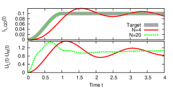
Figure 2: NQDN junction with an optimized current for two different numbers of spline nodes $N$. The parameters are: $\Gamma_{\alpha}=0.2,\epsilon_{\textnormal{QD}}=0.5,\xi_{\alpha}=0$.

The optimization of the density $n_{\textnormal{QD}}(t)$ is very similar to the optimization of a current, one simply exchanges the observable in the objective function. An example is shown in Fig 3. The density follows perfectly the target pattern.

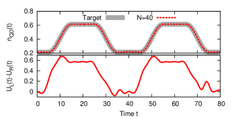
Figure 3: NQDN junction with an optimized density. The parameters are: $\Gamma_{\alpha}=0.2,\epsilon_{\textnormal{QD}}=0.5,\xi_{\alpha}=0$.

IV.2 Controlling classical vibrations

In this paragraph, we extend the model to incorporate a vibrational degree of freedom in the central region. In the past, most theoretical work focused on the electronic system and neglected the nuclear motion. In experiments, the nuclei are, of course, not fixed to a position and their motion can have a significant influence on the measured properties, for example on the current-voltage characteristics Galperin et al. (2007); Koch and von Oppen (2005); Ryndyk et al. (2006); Härtle et al. (2009).

The goal of this section is to control the nuclear motion using the bias as before. Although the bias couples only to the electronic part of the system, it induces changes in the density which in turn influences the nuclear motion. Hence, the electrons mediate between the bias and the vibration. The feasibility of controlling the nuclear motion in a quantum-classical system has already been demonstrated. Castro and Gross (2014)

The vibrational degree of freedom is described within the Ehrenfest approximation following Verdozzi et al. Verdozzi et al. (2006). The modified central part of the electronic Hamiltonian reads

$$\hat{H}_{\textnormal{QD}}(t)=(\epsilon_{\textnormal{QD}}+\lambda x(t))\sum_{\sigma\in\{\uparrow,\downarrow\}}\hat{d}_{\sigma}^{\dagger}\hat{d}_{\sigma}.$$ (21)

The parameter $\lambda$ determines the interaction strength between the electronic and the nuclear system. The equation of motion for the vibrational coordinate $x(t)$ is

$$m\partial_{t}^{2}x(t) =-\frac{\,d}{\,dx}\left(\frac{1}{2}m\omega^{2}x^{2}+\langle\Psi|\hat{H}_{\textnormal{QD}}(t)|\Psi\rangle\right)$$ (22)

$$=-m\omega^{2}x(t)-\lambda n_{\textnormal{QD}}(t),$$ (23)

$$x(0) =x^{0}.$$

The initial value $x^{0}$ is calculated self-consistently and the classical equation of motion for the vibrational degree of freedom is solved simultaneously with the time-dependent Schrödinger equation. The optimization problem for controlling the vibrational coordinate $x(t)$ then reads

$$\min_{\vec{u}_{\textnormal{L}},\vec{u}_{\textnormal{R}}\in\mathbb{R}^{N+1}}\|x(t)-x^{(\textnormal{target})}(t)\|_{2,[0,T]}^{2}\qquad\qquad\quad\$$ (24)

$$\begin{array}[]{rcl}\textnormal{s.t. }&&\\ i\partial_{t}\psi_{q}(t)&=&\mathbf{H}(\vec{u}_{\textnormal{L}},\vec{u}_{\textnormal{R}},x(t),t)\psi_{q}(t),t\in[0,T],\\ m\partial_{t}^{2}x(t)&=&-m\omega^{2}x(t)-\lambda n_{\textnormal{QD}}(t),t\in[0,T],\\ \psi_{q}(0)&=&\psi_{q}^{0},\\ x(0)&=&x^{0},\\ \vec{u}_{\textnormal{L}}&=&-\vec{u}_{\textnormal{R}},\\ U_{\alpha}(\vec{u}_{\alpha},\tau_{0})&=&0,\quad\alpha\in\{\textnormal{L},\textnormal{R}\}.\end{array}$$ (32)

Figure 4 shows the results of such a calculation.

Figure 4: NQDN junction with an optimized position $x(t)$ of a vibration coupled to the quantum dot. The parameters are: $\Gamma_{\alpha}=0.2,\epsilon_{\textnormal{QD}}=0.5,\xi_{\alpha}=0,\lambda=0.1,\omega=0.5,m=1$.

IV.3 Imposing further constraints on the bias

In real-world control experiments, an arbitrary time-dependence of $U_{\alpha}(t)$ is difficult to achieve. In this section, we therefore impose further constraints to restrict the bias $U_{\alpha}(t)$ or the derivative $\partial_{t}U_{\alpha}(t)$. The optimization problem including such additional constraints then reads

$$\min_{\vec{u}_{\textnormal{L}},\vec{u}_{\textnormal{R}}\in\mathbb{R}^{N+1}}\|O[\Psi](t)-O^{(\textnormal{target})}(t)\|_{2,[0,T]}^{2}\qquad\qquad$$ (33)

$$\begin{aligned} \textnormal{s.t. }\quad i\partial_{t}\psi_{q}(t)&=\mathbf{H}(\vec{u}_{\textnormal{L}},\vec{u}_{\textnormal{R}},t)\psi_{q}(t),\ t\in[0,T],\\ \psi_{q}(0)&=\psi_{q}^{0},\\ U_{\alpha}(\vec{u}_{\alpha},\tau_{0})&=0,\\ \vec{u}_{\textnormal{L}}&=-\vec{u}_{\textnormal{R}},\\ U_{\alpha}^{(\textnormal{min})}&\leq\ \ \ \ U_{\alpha}(\vec{u}_{\alpha},t)\leq U_{\alpha}^{(\textnormal{max})},\\ \widetilde{U}_{\alpha}^{(\textnormal{min})}&\leq\frac{\,d}{\,dt}U_{\alpha}(\vec{u}_{\alpha},t)\leq\widetilde{U}_{\alpha}^{(\textnormal{max})}.\end{aligned}$$

The conditions $U_{\alpha}^{(\textnormal{min})}\leq U_{\alpha}(\vec{u}_{\alpha},t)\leq U_{\alpha}^{(\textnormal{max})}$ are in general not equivalent to $U_{\alpha}^{(\textnormal{min})}\leq\vec{u}_{\alpha}\leq U_{\alpha}^{(\textnormal{max})}$, unless one uses a monotonic cubic spline. This can be seen in Fig 1, where the maximum value of the spline lies between $\tau_{1}$ and $\tau_{2}$. The constraint for the time derivative is not accessible in this way.

The cubic spline is a third degree polynomial between two nodes $\tau_{j}$ and $\tau_{j+1}$. Thus, the minimum and maximum values can be calculated analytically in every interval $[\tau_{j},\tau_{j+1}]$. The constraints are replaced by

$$\max_{t\in[\tau_{j},\tau_{j+1}]}U_{\alpha}(\vec{u}_{\alpha},t) \leq U_{\alpha}^{(\textnormal{max})},$$ (34)

$$\min_{t\in[\tau_{j},\tau_{j+1}]}U_{\alpha}(\vec{u}_{\alpha},t) \geq U_{\alpha}^{(\textnormal{min})},$$ (35)

$$\max_{t\in[\tau_{j},\tau_{j+1}]}\frac{\,d}{\,dt}U_{\alpha}(\vec{u}_{\alpha},t) \leq\widetilde{U}_{\alpha}^{(\textnormal{max})},$$ (36)

$$\min_{t\in[\tau_{j},\tau_{j+1}]}\frac{\,d}{\,dt}U_{\alpha}(\vec{u}_{\alpha},t) \geq\widetilde{U}_{\alpha}^{(\textnormal{min})}$$ (37)

for $j\in\{0,\ldots N-1\}$. Figure 5 shows the influence of the additional constraints. They are chosen such that the steady state value can still be reached, but the transient time is lengthened.

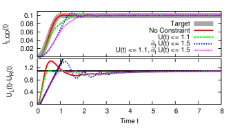
Figure 5: NQDN junction with an optimized current $I_{\textnormal{L,QD}}(t)$. The black lines represent the additional constraints $U(t)\leq 1.1$ and $\partial_{t}U(t)\leq 1.5$. The parameters are: $\Gamma_{\alpha}=0.2,\epsilon_{\textnormal{QD}}=0.5,\xi_{\alpha}=0,N=25$.

IV.4 Generating DC currents in Josephson junctions

When making the leads superconducting, a junction with an applied DC bias does not reach a steady state anymore, but ends up in a time-periodic state. A DC current, on the other hand, can flow through the junction even without applying a bias. These phenomena are known as the AC and DC Josephson effects Josephson (1962). The underlying relation is

$$U(t) =\frac{\hbar}{2e}\frac{\,d\chi}{\,dt},$$ (38)

$$\chi(0) =\chi_{\textnormal{R}}-\chi_{\textnormal{L}},$$ (39)

$$I(t) =I_{0}+I_{1}\sin(\chi(t))+I_{2}\cos(\chi(t)),$$ (40)

where the variables $\chi_{\alpha}$ describe the phase of the superconducting wave function in lead $\alpha$. Thus, the current oscillates with the frequency $\omega=\frac{2e}{\hbar}U$ when applying a constant bias $U$ across the junction. The values of $I_{0},I_{1}$ and $I_{2}$ depend on the bias and only $I_{1}$ is non-zero for zero bias. Following these equations, the only solution for a DC current flowing through the junction would be $\chi(t)\equiv\textnormal{const}$ and hence $U(t)=0$. But these equations do not take switching effects into account and only approximate the current after the transients. In order to force the current to follow a predefined pattern, one can make use of the reaction of the current to time-dependent changes in the bias. These can be used, for example, to compensate the Josephson oscillations.

We start again with optimizing the current $I_{\textnormal{L},\textnormal{{QD}}}(t)$ from the left lead onto the quantum dot such that it follows the target pattern. In this way, we generate a DC current $I_{\textnormal{L},\textnormal{{QD}}}(t)$. But the current $I_{\textnormal{QD},\textnormal{R}}(t)$ still shows the typical oscillation as it is shown in Fig 6.

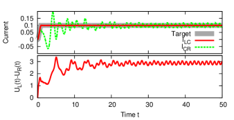
Figure 6: SQDS junction with an optimized current for two different number of spline nodes $N$. The parameters are: $\Gamma_{\alpha}=0.2,\epsilon_{\textnormal{QD}}=0.5,\xi_{\alpha}=1,\chi_{\alpha}=0$.

In order to obtain a real DC current flowing through the Josephson junction, one has to modify the objective function. The idea is to optimize $I_{\textnormal{L},\textnormal{{QD}}}(t)$ and $I_{\textnormal{QD},\textnormal{R}}(t)$ simultaneously such that each of them follows a target pattern. The targets have to be chosen carefully, since one might end up in situations where the targets cannot be reached simultaneously.

Suppose that the currents $I_{\textnormal{L},\textnormal{{QD}}}(t)$ and $I_{\textnormal{QD},\textnormal{R}}(t)$ follow the predefined patterns perfectly. The density on the quantum dot can then be obtained by integrating the continuity equation at the quantum dot:

$$n_{\textnormal{QD}}(t)=n_{\textnormal{QD}}(0)+\int_{0}^{t}\,dt^{\prime}\sum_{\alpha\in\{\textnormal{L},\textnormal{R}\}}I_{\alpha,\textnormal{QD}}^{(\textnormal{target})}(t^{\prime}).$$ (41)

As we see, this can easily lead to contradictions like $n_{\textnormal{QD}}(t)<0$ or $n_{\textnormal{QD}}(t)>2$, if the targets are not chosen carefully. Even situations with $I_{\textnormal{L},\textnormal{{QD}}}(t)=-I_{\textnormal{R},\textnormal{QD}}(t)\neq 0$ for all times $t$ are in general not possible, since the density in such cases would be constant, but switching on a bias normally changes the density.

We avoid these difficulties by using the norm $L^{2}([t_{0},t_{1}])$, $0\leq t_{0}<t_{1}\leq T$ in the objective function, which is denoted by $\|\cdot\|_{2,[t_{0},t_{1}]}$. Furthermore, we remove the constraint $U_{\textnormal{L}}(t)=-U_{\textnormal{R}}(t)$ in order to make the targets reachable. The modified optimization problem reads

$$\min_{\vec{u}_{\textnormal{L}},\vec{u}_{\textnormal{R}}\in\mathbb{R}^{N+1}} \left(\|I_{\textnormal{L},\textnormal{QD}}[\Psi](t)-I_{\textnormal{L},\textnormal{QD}}^{(\textnormal{target})}(t)\|_{2,[t_{0},t_{1}]}^{2}\right.$$ (42)

$$\left.+\|I_{\textnormal{QD},\textnormal{R}}[\Psi](t)-I_{\textnormal{QD},\textnormal{R}}^{(\textnormal{target})}(t)\|_{2,[t_{0},t_{1}]}^{2}\right)$$

$$\begin{matrix}\textnormal{s.t.}\\ \ \\ \ \end{matrix}\quad \begin{array}[]{rcl}i\partial_{t}\psi_{q}(t)&=&\mathbf{H}(\vec{u}_{\textnormal{L}},\vec{u}_{\textnormal{R}},t)\psi_{q}(t),\ t\in[0,T],\\ \psi_{q}(0)&=&\psi_{q}^{0},\\ U_{\alpha}(\vec{u}_{\alpha},\tau_{0})&=&0,\quad\alpha\in\{\textnormal{L},\textnormal{R}\}.\end{array}$$ (46)

The system has now the freedom to adjust the density and currents from time $0$ to $t_{0}$ such that the target patterns can be reached. There are two ways to achieve a DC current flowing through a Josephson junction:

1. Following the equations (38) - (40), only the case $U(t)=0$ produces a DC current, namely $I(t)=I_{1}\sin(\chi_{0})$. This is the DC Josephson effect. In general, this relation is not true for our model, since the quantum dot always supports two Andreev bound states for $U=0$ Stefanucci et al. (2010). They lead to persistent oscillations in the current and density Stefanucci (2007); Khosravi et al. (2008); Stefanucci et al. (2010). The oscillations in the current can be compensated by small variations of the bias $U(t)=U_{\textnormal{L}}(t)-U_{\textnormal{R}}(t)$ around the origin. Figure 7 shows an example of such a solution. This approach is limited by $I_{1}$ and hence does not work for arbitrary large DC currents.

2. An alternative approach is to apply a DC bias across the junction, leading to a linear increase in the phase difference $\chi(t)$ and thus to oscillations in the currents. This is the AC Josephson effect. These oscillations can be compensated again by small variations in the bias, the reaction to these changes cancels the Josephson oscillations. Figure 8 shows an example for this type of solutions.

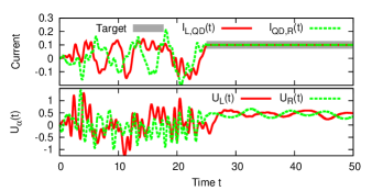
Figure 7: SQDS junction with optimized currents $I_{\textnormal{L},\textnormal{QD}}(t)$ and $I_{\textnormal{QD},\textnormal{R}}(t)$. We remove the constraint $U_{\textnormal{L}}(t)=-U_{\textnormal{R}}(t)$ since the target can not be reached otherwise. The target is the same for both currents and starts at $t=25$. The solution exploits the DC Josephson effect. The parameters are: $\Gamma_{\alpha}=0.2,\epsilon_{\textnormal{QD}}=0.5,\xi_{\alpha}=1,\chi_{\alpha}=0,t_{0}=25,t_{1}=50$.

Figure 8: Same junction as in Fig 7, but a different solution to the problem. This solution exploits the AC Josephson effect.

V Optimizing the Cooper pair splitting efficiency

In this section, we demonstrate how to optimize the Cooper pair splitting efficiency in a two-quantum dot Y-junction. The overall idea is to create entangled electrons at two quantum dots.

The entanglement of quantum particles has fascinated the scientific community since the proposition of the Einstein-Podolsky-Rosen (EPR) Gedankenexperiment Einstein et al. (1935). Entanglement means that two particles are linked such that the measurement of one particle is sufficient to completely determine the quantum state of the other one. A prominent example is a pair of electrons with opposite spin. Suppose, you have a pair of entangled electron in a spin singlet. Then, one spin is up and the other spin is always pointing downwards. Photons are a second example which can be entangled with respect to the polarization.

The EPR Gedankenexperiment is directly linked to the question of non-locality of quantum mechanics: Can a measurement at position $x$ have an influence on a simultaneous or later independent measurement at a different position $x^{\prime}$? This question can be cast into a mathematical formula known as Bell’s inequality Bell (1964). A violation of the latter would prove the non-locality of quantum mechanics.

Great progress has been achieved with entangled photons, but the final experiment ruling out all possible loopholes has not yet been accomplished Giustina et al. (2013). For example, the two measurements at $(x,t)$ and $(x^{\prime},t^{\prime})$ have to be separated such that $c|t-t^{\prime}|<\|x-x^{\prime}\|$, i.e. no information of the first measurement can be transmitted to the second. Hence large distances are typically required to close this loophole Weihs et al. (1998). Another important loophole stems from the detector efficiency, i.e. one has to take into account that undetected particles might behave completely different compared to the detected ones. Typically, one uses the fair sampling assumption stating that the detected particles are selected randomly and behave statistically in the same way as the undetected ones.

To do similar Bell test experiments with electrons is much more difficult and remains an open challenge. In recent years, a number of ingenious experiments to create entangled electrons have been performed Hofstetter et al. (2009, 2011); Herrmann et al. (2010); Schindele et al. (2012), going along with several theoretical developments Recher et al. (2001); Recher and Loss (2002); Sauret et al. (2004); Morten et al. (2006); Golubev and Zaikin (2007); Burset et al. (2011). The basic idea is to use a superconductor as a source of entangled electrons. In the BCS ground state, electrons form Cooper pairs due to the attractive interaction caused by phonons. These pairs consist of two electrons with opposite spin and momentum.

The idea is to create a splitted Cooper pair at the two quantum dots, i.e. one electron is on the left quantum dot and the other with opposite spin is on the right one (see sketch in Fig. 9). However, this process competes with the case of both electrons moving onto the same quantum dot. The latter can be suppressed by a large charging energy of the quantum dots caused by the Coulomb interaction. This make double occupancies less likely.

We propose a way to achieve splitting efficiencies of $99\%$ and more, which we hope will help the eventual experimental demonstration of the violation of Bell’s inequality. In comparison to traditional approaches, our method has two major differences. First, we do not rely on a large Coulomb repulsion on the quantum dots but rather use optimal control theory to tailor the bias in the normal leads in such a way that the splitting probability is maximized. Second, we look at the Cooper pair density on the quantum dots as opposed to the experimental approaches working currents of entangled electrons in the two normal conducting leads. Consequently, a direct comparison of results is not easily possible as the efficiencies measure different ratios. As a future work, it might be worth doing an extensive comparative study answering whether the here created pair eventually moves towards the leads or stays on the quantum dots. In experiments, splitting efficiencies for the current of $90\%$ have been realized in recent experiments Schindele et al. (2012) being significantly higher than previous results. Despite this progress, the experimental proof of the violation of Bell’s inequality is still pending.

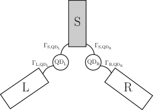
Figure 9: Sketch of the Y junction and explanation of all relevant parameters. Only the lead labeled with S is superconducting. The gray color is used to indicate the superconducting part. The aim is to create entangled electrons on the two quantum dots. All three leads are semi infinite.

In contrast to all systems studied in the previous sections, we now work with three leads. The system is sketched in Fig 9. It consists of two quantum dots ($\textnormal{QD}_{\textnormal{L}}$ and $\textnormal{QD}_{\textnormal{R}}$), one superconducting (S) and two normal leads (L and R).

The Hamiltonian of our modified model reads

$$\hat{H}(t) =\sum_{\alpha\in\{\textnormal{L},\textnormal{R},\textnormal{S}\}}\hat{H}_{\alpha}+\sum_{\alpha\in\{\textnormal{L},\textnormal{R},\textnormal{S}\}}\hat{H}_{T,\alpha}(t),$$ (47)

$$\hat{H}_{\alpha} =\sum_{k=0}^{\infty}\sum_{\sigma\in\{\uparrow,\downarrow\}}\left(t_{\alpha}\hat{c}_{\alpha k\sigma}^{\dagger}\hat{c}_{\alpha(k+1)\sigma}+H.c.\right)$$ (48)

$$\qquad+\sum_{k=0}^{\infty}\left(\Delta_{\alpha}e^{i\chi_{\alpha}}\hat{c}_{\alpha k\uparrow}^{\dagger}\hat{c}_{\alpha k\downarrow}^{\dagger}+H.c.\right),$$

$$\hat{H}_{T,S}(t) =\sum_{\alpha\in\{\textnormal{L},\textnormal{R}\}}\sum_{\sigma\in\{\uparrow,\downarrow\}}\left(t_{\textnormal{S},\textnormal{QD}_{\alpha}}\hat{c}_{\textnormal{S}0\sigma}^{\dagger}\hat{d}_{\textnormal{QD}_{\alpha}\sigma}+H.c.\right),$$ (49)

$$\hat{H}_{T,\alpha}(t) =\sum_{\sigma\in\{\uparrow,\downarrow\}}\left(t_{\alpha,\textnormal{QD}_{\alpha}}e^{i\gamma_{\alpha,\textnormal{QD}_{\alpha}}(t)}\hat{c}_{\alpha 0\sigma}^{\dagger}\hat{d}_{\textnormal{QD}_{\alpha}\sigma}+H.c.\right)$$

$$\qquad\qquad\qquad\textnormal{for }\alpha\in\{\textnormal{L},\textnormal{R}\}.$$ (50)

Note that there is only a bias in the left and right lead. All parameters are again chosen real and positive. Furthermore, we work at temperature $T=0$ and assume the wide band limit $t_{\alpha,\textnormal{QD}_{\beta}}\ll t_{\alpha}$. Again, only the coupling strengths $\Gamma_{\alpha,\textnormal{QD}_{\beta}}={2t_{\alpha,\textnormal{QD}_{\beta}}^{2}}/{t_{\alpha}}$ will be stated.

In the following, we demonstrate how to optimize the Cooper pair splitting efficiency in the above model of a two-quantum dot Y-junction. The goal is to operate the device as a Cooper pair splitter that creates entangled electrons on the two quantum dots. The splitting of a Cooper pair can be understood as a crossed Andreev reflection. An incoming electron in one of the normal leads gets reflected into the other lead as a hole. This creates a Cooper pair in the superconductor. The process is sketched in Fig. 10 (top left). Similarly, the opposite process removes a Cooper pair from the superconductor. Besides, there are three other possible reflection processes: (a) normal reflection, (b) Andreev reflection, and (c) elastic cotunneling. The latter corresponds to a reflection of the incoming electron to the opposite lead. These three processes together with the crossed Andreev reflection are all sketched in Fig. 10.

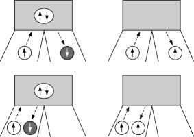
Figure 10: Overview of the four possible reflection processes. Black arrows indicate electrons, white arrows represent holes. The gray block is the superconducting lead S of Fig. 9. Top left: Sketch of a crossed Andreev reflection. The incoming spin up electron in the left lead gets reflected as a spin down hole to the right lead. Simultaneously, a Cooper pair is created in the superconducting lead. The opposite process, which removes a Cooper pair from the superconductor, is also possible. Bottom left: The reflected hole stays in the left lead. This corresponds to the normal Andreev reflection. Top right: Sketch of an elastic cotunneling process. Now, the incoming electron gets reflected into the right lead. Bottom right: Alternatively, the electron can also be reflected into the left lead corresponding to normal reflection.

The central ingredient for the optimization process is the proper definition of a suitable objective function which is then to be maximized. It has to quantify the Cooper pair splitting efficiency. To this end, we first define the so-called pairing density or anomalous density as

$$P_{\textnormal{QD}_{\alpha},\textnormal{QD}_{\beta}}(t) =\langle\hat{d}_{\textnormal{QD}_{\alpha}\downarrow}(t)\hat{d}_{\textnormal{QD}_{\beta}\uparrow}(t)\rangle.$$ (51)

We use its absolute value squared $|P_{\textnormal{QD}_{\alpha},\textnormal{QD}_{\beta}}(t)|^{2}$ as a measure for the Cooper pair density with one electron at $\textnormal{QD}_{\alpha}$ and the other at $\textnormal{QD}_{\beta}$. We propose to maximize the following objective function:

$$\frac{1}{t_{1}-t_{0}}\int_{t_{0}}^{t_{1}}\,dt\frac{\sum_{\alpha\neq\alpha^{\prime}\in\{\textnormal{L},\textnormal{R}\}}|P_{\textnormal{QD}_{\alpha},\textnormal{QD}_{\alpha^{\prime}}}(t)|^{2}}{\sum_{\alpha,\alpha^{\prime}\in\{\textnormal{L},\textnormal{R}\}}|P_{\textnormal{QD}_{\alpha},\textnormal{QD}_{\alpha^{\prime}}}(t)|^{2}}.$$ (52)

The fraction represents the Cooper pair splitting efficiency at time t, which is expressed as the amount of Cooper pairs being split up divided by the total amount of Cooper pairs on the quantum dots. We calculate its average over the time span from $t_{0}$ to $t_{1}$. The pairing densities $P_{\textnormal{QD}_{\alpha},\textnormal{QD}_{\beta}}(t)$ are obtained from the single particle wave functions $\psi_{q}(t)$, i.e., the solutions of the time-dependent Bogoliubov-de Gennes equation (7).

We want to tailor the bias such that we maximize the time averaged Cooper pair splitting efficiency. The corresponding optimization problem then reads

$$\max_{\vec{u}_{\textnormal{L}},\vec{u}_{\textnormal{R}}\in\mathbb{R}^{N+1}}\frac{1}{t_{1}-t_{0}}\int_{t_{0}}^{t_{1}}\,dt\frac{\sum_{\alpha\neq\alpha^{\prime}\in\{\textnormal{L},\textnormal{R}\}}|P_{\textnormal{QD}_{\alpha},\textnormal{QD}_{\alpha^{\prime}}}(t)|^{2}}{\sum_{\alpha,\alpha^{\prime}\in\{\textnormal{L},\textnormal{R}\}}|P_{\textnormal{QD}_{\alpha},\textnormal{QD}_{\alpha^{\prime}}}(t)|^{2}}$$

$$\begin{array}[]{rcl}\textnormal{s.t. }P_{\textnormal{QD}_{\alpha},\textnormal{QD}_{\beta}}(t)&=&\int\,dqf(\epsilon_{q})u_{q}(\textnormal{QD}_{\alpha},t)v_{q}(\textnormal{QD}_{\beta},t)^{\star},\\ \quad i\partial_{t}\psi_{q}(t)&=&\mathbf{H}(\vec{u}_{\textnormal{L}},\vec{u}_{\textnormal{R}},t)\psi_{q}(t),\quad t\in[0,T],\\ \psi_{q}(0)&=&\psi_{q}^{0},\\ U_{\alpha}(\vec{u}_{\alpha},\tau_{0})&=&0,\quad\alpha\in\{\textnormal{L},\textnormal{R}\}.\end{array}$$ (57)

The problem can be solved using again standard derivative-free algorithms for non-linear optimization problems, for example the ones provided by the library NLopt Johnson .

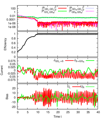
Figure 11: Simulation with an optimized bias. (a) Top: $|P_{\textnormal{QD}_{\alpha},\textnormal{QD}_{\beta}}(t)|^{2}$ as a function of time. (b) Second from top: Resulting efficiency, gray line indicates time interval of optimization. second from bottom (c) Second from bottom: Resulting currents $I_{\textnormal{QD}_{\textnormal{L}},\textnormal{S}}(t)$ and $I_{\textnormal{S},\textnormal{QD}_{\textnormal{R}}}(t)$. (d) Bottom: Tailored bias $U_{\textnormal{L}}(t)$ and $U_{\textnormal{R}}(t)$ of the optimization. The parameters are: $\Gamma_{\textnormal{S},\textnormal{QD}_{\textnormal{L}}}=\Gamma_{\textnormal{S},\textnormal{QD}_{\textnormal{R}}}=\Gamma_{\textnormal{N},\textnormal{QD}_{\textnormal{L}}}=0.2$, $\Gamma_{\textnormal{N},\textnormal{QD}_{\textnormal{R}}}=1$, $\xi_{\textnormal{S}}=1$, $\xi_{\textnormal{L}}=\xi_{\textnormal{R}}=0$, $N=200$.

To achieve high splitting efficiencies it is essential that the junction is asymmetric, i.e. the couplings to the left and to the right quantum dot must not be equal. This is necessary since we observe an upper bound of $50\%$ for the Cooper pair splitting efficiency in symmetric junctions, which is already achieved in the ground state by the usual Cooper pair tunneling leading to the proximity effect. Hence any optimization starting in the ground state will not improve the results. The underlying cause for this limitation is still unknown and under investigation. In order to bypass this issue, we choose an asymmetric coupling of the quantum dots to the normal leads.

The results of such an optimization are depicted in Fig. 11. The bias is tailored such that the Cooper pair splitting efficiency is maximized. It suppresses the non-splitting processes. The efficiency is optimized in the time interval from $t_{0}=10$ to $t_{1}=40$. This interval is indicated by the underlying thick gray line in the plot of the efficiency (second from top). In this interval, we achieve an average efficiency of more than $99\%$. The values of $|P_{\textnormal{QD}_{\textnormal{L}},\textnormal{QD}_{\textnormal{R}}}(t)|^{2}$ and $|P_{\textnormal{QD}_{\textnormal{R}},\textnormal{QD}_{\textnormal{L}}}(t)|^{2}$ are on top of each other. The resulting currents flowing through the junction indicate, that in the time average, there is a net current flowing from the right normal conducting lead (R) via the superconductor (S) to the left one (L). This is deduced from the observation that $I_{\textnormal{QD}_{\textnormal{L}},\textnormal{S}}(t)$ and $I_{\textnormal{S},\textnormal{QD}_{\textnormal{R}}}(t)$ are both negative in the time average. We point out, that this does not say anything about the movement of the entangled Cooper pairs.

This result clearly demonstrates that the Coulomb interaction at the quantum dots is not necessary in order to obtain high efficiencies. One can also succeed with optimized biases.

VI Conclusion

Usually, in the field of molecular electronics, the goal is to calculate the steady-state or time-dependent current that is generated by a given bias and gate voltage. Sometimes, however, one may be interested in taking a step beyond this point and control the current or other observables of the junction. To this end we have presented an algorithm that allows us to calculate the time-dependent bias that achieves a prescribed goal. In the examples presented, we determine numerically the time-dependent bias that forces the current, the density or the molecular vibration to follow a given temporal pattern. The method is general and not restricted to the observables listed above. In the final section we apply our approach to optimize the Cooper pair splitting efficiency in a Y-junction with two quantum dots. We successfully create spatially separated entangled electron pairs with an efficiency of nearly 100%. We expect our approach to be useful in the control of other - essentially arbitrary - observables in molecular junctions.

References

- Aviram and Ratner (1974) A. Aviram and M. A. Ratner, Chemical Physics Letters 29, 277 (1974).
- Cuniberti et al. (2005) G. Cuniberti, G. Fagas, and K. Richter, Introducing Molecular Electronics (Springer, 2005).
- Di Ventra (2008) M. Di Ventra, Electrical Transport in Nanoscale Systems, 1st ed. (Cambridge University Press, 2008).
- Cuevas and Scheer (2010) J. C. Cuevas and E. Scheer, Molecular Electronics (World Scientific Publishing Company, 2010).
- Runge and Gross (1984) E. Runge and E. K. U. Gross, Physical Review Letters 52, 997 (1984).
- Baer et al. (2004) R. Baer, T. Seideman, S. Ilani, and D. Neuhauser, The Journal of chemical physics 120, 3387 (2004).
- Burke et al. (2005) K. Burke, R. Car, and R. Gebauer, Physical Review Letters 94, 146803+ (2005).
- Kurth et al. (2005) S. Kurth, G. Stefanucci, C. O. Almbladh, A. Rubio, and E. K. U. Gross, Physical Review B 72, 035308+ (2005).
- Yuen-Zhou et al. (2009) J. Yuen-Zhou, C. Rodriguez-Rosario, and A. Aspuru-Guzik, Phys. Chem. Chem. Phys. 11, 4509 (2009).
- Di Ventra and D’Agosta (2007) M. Di Ventra and R. D’Agosta, Physical Review Letters 98, 226403+ (2007).
- Appel and Di Ventra (2009) H. Appel and M. Di Ventra, Physical Review B 80, 212303+ (2009).
- Appel and Di Ventra (2011) H. Appel and M. Di Ventra, Chemical Physics 391, 27 (2011).
- Stefanucci and van Leeuwen (2013) G. Stefanucci and R. van Leeuwen, Nonequilibrium Many-Body Theory of Quantum Systems: A Modern Introduction (Cambridge University Press, 2013).
- Myöhänen et al. (2009) P. Myöhänen, A. Stan, G. Stefanucci, and R. van Leeuwen, Physical Review B 80, 115107+ (2009).
- Myöhänen et al. (2010) P. Myöhänen, A. Stan, G. Stefanucci, and R. van Leeuwen, Journal of Physics: Conference Series 220, 012017+ (2010).
- Knap et al. (2011) M. Knap, W. von der Linden, and E. Arrigoni, Physical Review B 84, 115145+ (2011).
- Zanghellini et al. (2004) J. Zanghellini, M. Kitzler, T. Brabec, and A. Scrinzi, Journal of Physics B: Atomic, Molecular and Optical Physics 37, 763+ (2004).
- Wang and Thoss (2009) H. Wang and M. Thoss, The Journal of Chemical Physics 131, 024114+ (2009).
- Wang and Thoss (2013) H. Wang and M. Thoss, J. Phys. Chem. A 117, 7431 (2013).
- Albrecht et al. (2012) K. F. Albrecht, H. Wang, L. Mühlbacher, M. Thoss, and A. Komnik, Physical Review B 86, 081412+ (2012).
- Mühlbacher and Rabani (2008) L. Mühlbacher and E. Rabani, Physical Review Letters 100, 176403+ (2008).
- Wang et al. (2011) Y. Wang, C. Y. Yam, T. Frauenheim, G. H. Chen, and T. A. Niehaus, Chemical Physics 391, 69 (2011).
- Zhang et al. (2013) Y. Zhang, S. Chen, and G. H. Chen, Physical Review B 87, 085110+ (2013).
- Oppenländer et al. (2013) C. Oppenländer, B. Korff, T. Frauenheim, and T. A. Niehaus, Phys. Status Solidi B 250, 2349 (2013).
- Jin et al. (2008) J. Jin, X. Zheng, and Y. Yan, The Journal of Chemical Physics 128, 234703+ (2008).
- Zheng et al. (2008a) X. Zheng, J. Jin, and Y. Yan, New Journal of Physics 10, 093016+ (2008a).
- Zheng et al. (2008b) X. Zheng, J. Jin, and Y. Yan, The Journal of Chemical Physics 129, 184112+ (2008b).
- Pontryagin et al. (1962) L. S. Pontryagin, V. G. Boltyanskii, R. V. Gamkrelidze, and E. F. Mishchenko, Mathematical Theory of Optimal Processes (John Wiley & Sons, New York/London, 1962).
- Bellman (1957) R. Bellman, Dynamic programming (Princeton University Press, 1957).
- Peirce et al. (1988) A. P. Peirce, M. A. Dahleh, and H. Rabitz, Physical Review A 37, 4950 (1988).
- Shenghua et al. (1988) S. Shenghua, A. Woody, and H. Rabitz, The Journal of Chemical Physics 88, 6870 (1988).
- Kosloff et al. (1989) R. Kosloff, S. A. Rice, P. Gaspard, S. Tersigni, and D. J. Tannor, Chemical Physics 139, 201 (1989).
- Assion et al. (1998) A. Assion, T. Baumert, M. Bergt, T. Brixner, B. Kiefer, V. Seyfried, M. Strehle, and G. Gerber, Science 282, 919 (1998).
- Hartke et al. (1989) B. Hartke, J. Manz, and J. Mathis, Chemical Physics 139, 123 (1989).
- Elghobashi et al. (2003) N. Elghobashi, P. Krause, J. Manz, and M. Oppel, Physical Chemistry Chemical Physics 5, 4806 (2003).
- Elghobashi and Gonzalez (2004) N. Elghobashi and L. Gonzalez, Physical Chemistry Chemical Physics 6, 4071+ (2004).
- Levis et al. (2001) R. J. Levis, G. M. Menkir, and H. Rabitz, Science 292, 709 (2001).
- Räsänen et al. (2007) E. Räsänen, A. Castro, J. Werschnik, A. Rubio, and E. K. U. Gross, Physical Review Letters 98, 157404+ (2007).
- Reich and Koch (2013) D. M. Reich and C. P. Koch, New Journal of Physics 15, 125028+ (2013).
- Räsänen et al. (2012) E. Räsänen, T. Blasi, M. F. Borunda, and E. J. Heller, Physical Review B 86, 205308+ (2012).
- Räsänen and Heller (2013) E. Räsänen and E. J. Heller, The European Physical Journal B, 86, 1 (2013).
- Castro et al. (2009) A. Castro, E. Räsänen, A. Rubio, and E. K. U. Gross, EPL (Europhysics Letters) , 53001+ (2009).
- Räsänen and Madsen (2012) E. Räsänen and L. B. Madsen, Physical Review A 86, 033426+ (2012).
- Jakubetz et al. (1990) W. Jakubetz, J. Manz, and H. J. Schreier, Chemical Physics Letters 165, 100 (1990).
- Li et al. (2007) G. Q. Li, M. Schreiber, and U. Kleinekathöfer, EPL (Europhysics Letters) , 27006+ (2007).
- Amin et al. (2009) A. F. Amin, G. Q. Li, A. H. Phillips, and U. Kleinekathöfer, The European Physical Journal B 68, 103 (2009).
- Li and Kleinekathöfer (2010) G. Q. Li and U. Kleinekathöfer, The European Physical Journal B 76, 309 (2010).
- Stefanucci et al. (2010) G. Stefanucci, E. Perfetto, and M. Cini, Physical Review B 81, 115446+ (2010).
- Zhu et al. (1998) W. Zhu, J. Botina, and H. Rabitz, The Journal of Chemical Physics 108, 1953 (1998).
- Sklarz and Tannor (2002) S. E. Sklarz and D. J. Tannor, Physical Review A 66, 053619+ (2002).
- Palao and Kosloff (2003) J. P. Palao and R. Kosloff, Physical Review A 68, 062308+ (2003).
- Krieger et al. (2011) K. Krieger, A. Castro, and E. K. U. Gross, Chemical Physics 391, 50 (2011).
- Hellgren et al. (2013) M. Hellgren, E. Räsänen, and E. K. U. Gross, Physical Review A 88, 013414+ (2013).
- Räsänen et al. (2013) E. Räsänen, A. Putaja, and Y. Mardoukhi, Central European Journal of Physics, Central European Journal of Physics 11, 1066 (2013).
- Judson and Rabitz (1992) R. S. Judson and H. Rabitz, Physical Review Letters 68, 1500 (1992).
- Powell (2009) M. J. D. Powell, Department of Applied Mathematics and Theoretical Physics, Cambridge England, technical report NA2009/06 (2009).
- Powell (1994) M. J. D. Powell, in Advances in Optimization and Numerical Analysis, Vol. 275, edited by S. Gomez and J.-P. Hennart (1994) pp. 51–67.
- Powell (1998) M. J. D. Powell, Acta Numerica 7, 287 (1998).
- (59) S. G. Johnson, “The nlopt nonlinear-optimization package: http://ab-initio.mit.edu/nlopt.” .
- Galperin et al. (2007) M. Galperin, M. A. Ratner, and A. Nitzan, Journal of Physics: Condensed Matter 19, 103201+ (2007).
- Koch and von Oppen (2005) J. Koch and F. von Oppen, Physical Review Letters 94, 206804+ (2005).
- Ryndyk et al. (2006) D. A. Ryndyk, M. Hartung, and G. Cuniberti, Physical Review B 73, 045420+ (2006).
- Härtle et al. (2009) R. Härtle, C. Benesch, and M. Thoss, Physical Review Letters 102, 146801+ (2009).
- Castro and Gross (2014) A. Castro and E. K. U. Gross, Journal of Physics A: Mathematical and Theoretical 47, 025204+ (2014).
- Verdozzi et al. (2006) C. Verdozzi, G. Stefanucci, and C. O. Almbladh, Physical Review Letters 97, 046603+ (2006).
- Josephson (1962) B. D. Josephson, Physics Letters 1, 251 (1962).
- Stefanucci (2007) G. Stefanucci, Physical Review B 75, 195115+ (2007).
- Khosravi et al. (2008) E. Khosravi, S. Kurth, G. Stefanucci, and E. K. U. Gross, Applied Physics A 93, 355+ (2008).
- Einstein et al. (1935) A. Einstein, B. Podolsky, and N. Rosen, Physical Review 47, 777 (1935).
- Bell (1964) J. S. Bell, Physics 1, 195 (1964).
- Giustina et al. (2013) M. Giustina, A. Mech, S. Ramelow, B. Wittmann, J. Kofler, J. Beyer, A. Lita, B. Calkins, T. Gerrits, S. W. Nam, R. Ursin, and A. Zeilinger, Nature 497, 227 (2013).
- Weihs et al. (1998) G. Weihs, T. Jennewein, C. Simon, H. Weinfurter, and A. Zeilinger, Physical Review Letters 81, 5039 (1998).
- Hofstetter et al. (2009) L. Hofstetter, S. Csonka, J. Nygard, and C. Schönenberger, Nature 461, 960 (2009).
- Hofstetter et al. (2011) L. Hofstetter, S. Csonka, A. Baumgartner, G. Fülöp, S. d’Hollosy, J. Nygård, and C. Schönenberger, Physical Review Letters 107, 136801+ (2011).
- Herrmann et al. (2010) L. G. Herrmann, F. Portier, P. Roche, A. Levy Yeyati, T. Kontos, and C. Strunk, Physical Review Letters 104, 026801+ (2010).
- Schindele et al. (2012) J. Schindele, A. Baumgartner, and C. Schönenberger, Physical Review Letters 109, 157002+ (2012).
- Recher et al. (2001) P. Recher, E. V. Sukhorukov, and D. Loss, Physical Review B 63, 165314+ (2001).
- Recher and Loss (2002) P. Recher and D. Loss, Journal of Superconductivity 15, 49 (2002).
- Sauret et al. (2004) O. Sauret, D. Feinberg, and T. Martin, Physical Review B 70, 245313+ (2004).
- Morten et al. (2006) J. P. Morten, A. Brataas, and W. Belzig, Physical Review B 74, 214510+ (2006).
- Golubev and Zaikin (2007) D. S. Golubev and A. D. Zaikin, Physical Review B 76, 184510+ (2007).
- Burset et al. (2011) P. Burset, W. J. Herrera, and A. Levy Yeyati, Physical Review B 84, 115448+ (2011).