More pieces of the puzzle: Chemistry and substructures in the Galactic thick disk

Abstract

We present a study of the chemical abundances of Solar neighbourhood stars associated to dynamical structures in the Milky Way’s (thick) disk. These stars were identified as overdensity in the eccentricity range $0.3<\epsilon<0.5$ in the Copenhagen-Geneva Survey by Helmi et al. (2006). We find that the stars with these dynamical characteristics do not constitute a homogeneous population. A relatively sharp transition in dynamical and chemical properties appears to occur at a metallicity of ${\rm[Fe/H]}\sim-0.4$. Stars with ${\rm[Fe/H]}>-0.4$ have mostly lower eccentricities, smaller vertical velocity dispersions, are $\alpha$-enhanced and define a rather narrow sequence in ${\rm[\alpha/Fe]}$ vs ${\rm[Fe/H]}$, clearly distinct from that of the thin disk. Stars with ${\rm[Fe/H]}<-0.4$ have a range of eccentricities, are hotter vertically, and depict a larger spread in ${\rm[\alpha/Fe]}$. We have also found tentative evidence of substructure possibly associated to the disruption of a metal-rich star cluster. The differences between these populations of stars is also present in e.g. ${\rm[Zn/Fe]}$, ${\rm[Ni/Fe]}$ and ${\rm[SmII/Fe]}$, suggesting a real physical distinction.

1 Introduction

In the concordance $\Lambda$CDM cosmological model, mergers are ubiquitous, and expected to have left imprints in galaxies like the Milky Way (Helmi & White, 1999; Bullock & Johnston, 2005). Although the majority of stars in disks have probably formed in situ, some fraction may originate in accreted objects on low inclination orbits (e.g. Abadi et al., 2003). Some evidence of such events may be the Monoceros ring in the outskirts of our Galaxy (Newberg et al., 2002, although its origin is still debated), the low-latitude substructures in M31 (Richardson et al., 2008), the Arcturus stream (Navarro et al., 2004), the $\omega$Cen stream (Meza et al., 2005; Majewski et al., 2012), and the groups found by Helmi et al. (2006, hereafter H06) and Arifyanto & Fuchs (2006) near the Sun.

The recovery of such events is the focus of many surveys, and correspondingly, attention has been given to the optimal search techniques. Most of the substructures discovered thus far have been identified in projections of phase-space, namely spatially (e.g. Belokurov et al., 2006), kinematically (Gilmore et al., 2002) or in an “integrals of motion” space (Helmi et al., 1999). However, there is the intriguing suggestion that merger debris may also be identifiable through peculiar chemical abundance patterns (Freeman & Bland-Hawthorn, 2002; De Silva et al., 2007), as stars formed in a common system must have experienced similar star formation and enrichment histories. Some first detections of chemically peculiar sequences or clustering have been reported by Nissen & Schuster (2010, 2011) and Wylie-de Boer et al. (2010, 2012).

In this Paper we present chemical abundances for a sample of nearby stars from the Copenhagen-Geneva survey found to define an overdensity in the eccentricity range $0.3\leq\epsilon\leq 0.5$ by H06 . We have performed a high-resolution follow-up study of 72 of these stars, and have supplemented this dataset with that of Stonkutė et al. (2012, 2013, hereafter ST) of 21 stars in the same overdensity. As we shall see below, a few subpopulations of stars with different dynamics and chemical abundances co-exist in this region of Galactic (extended) phase-space.

2 Observations and Analysis

2.1 The puzzle stars

The stars in H06 were identified in the Copenhagen-Geneva survey (Nordström et al., 2004, GCS hereafter), because of their peculiar distribution in the space of orbital apocentre-pericentre and $z$-component of the angular momentum. These stars share similar relatively planar orbits with moderate eccentricities between 0.3 and 0.5. This eccentricity region is overdense with respect to what is expected for a smooth model of the Galaxy (see Figures 10, 11 and 13 of H06). Besides their characteristic dynamics, the 274 stars identified were found to have distinct metallicity and age distributions. A separation into three different Groups was proposed on the basis of their metallicity, namely G1: $-0.45\!<\!{\rm[Fe/H]}\!<\!-0.2$ dex, G2: $\langle{\rm[Fe/H]}\rangle\!\sim\!-0.6$ dex, and G3: ${\rm[Fe/H]}\!<\!-0.7$ dex, where as the metallicity decreases, there is a tendency for the groups to have larger mean eccentricity. Group G2 has some overlap with the Arcturus stream, in terms of its average $V$ velocity and mean ${\rm[Fe/H]}$. Note that these ${\rm[Fe/H]}$ were estimated from Strömgren photometry and are slightly different from those derived here.

Figure 1 shows the velocity distribution of the revised GCS (Holmberg et al., 2009) highlighting the H06 stars. The stars included in this Paper are indicated with solid symbols (those we followed up with high-resolution spectroscopy), or with crosses (those from ST).

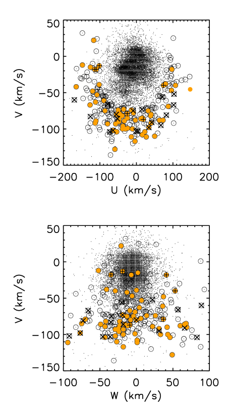
Figure 1: Velocities of stars in the revised GCS catalog, highlighting those from H06 . The solid symbols correspond to those we followed up with high-resolution spectroscopy, while the crosses are from ST. We have kept only stars with revised eccentricities $0.275\leq\epsilon\leq 0.525$. The stars with “+” symbols are those in the “tentative” cluster (see main text).

2.2 Derivation of chemical abundances

We performed our high signal-to-noise high-resolution spectroscopic study using UCLES on the 4m Anglo Australian Telescope. It includes 36 members of G1 (27.5% of all candidates identified by H06 ), 22 members of G2 (25.6%), and 14 members of G3 (20.6%). The wavelength coverage for our observations was $3850$ - $5300\textrm{\AA}$ and at least three exposures of on average $400\ \textrm{s}$ were done per star at a resolution $R\sim 45,000$. A signal-to-noise of $\sim 100-150$ per pixel at the central wavelength was obtained. The data were reduced using the standard IRAF routines ccdred and echelle, which included bias subtraction, flat-fielding, order extraction, scattered light subtraction and wavelength calibration. We focus here on those stars with $(V-K)>1.4$. Furthermore, two stars in G1 have significantly different eccentricities in the revised GCS, so we do not consider these further. We are thus left with a total of 64 stars: 30 from G1, 21 from G2 and 13 from G3.

To supplement this sample we also consider the 21 stars originally in G3 followed up by ST. Two of these have also been observed by us, and 3 have significantly revised GCS eccentricities which place them outside of the region of interest. We are therefore left with 16 independent stars from this sample.

Elemental abundances were derived for our stars by performing a Local Thermodynamic Equilibrium (LTE) analysis with the MOOG code (Sneden, 1973). To measure equivalent widths we used a modified version of the DAOSPEC program which automatically fits Gaussian profiles to lines in a spectrum (Stetson & Pancino, 2008). The modifications involved disabling DAOSPEC’s continuum fitting, and instead performing hand-fitting for our crowded blue data. In this Paper we present the abundances for our stars using stellar parameters calculated using a ‘spectroscopic’ (rather than physical) approach as they yielded better agreement for stars in common with external studies by Reddy et al. (2003, 2006) and Bensby et al. (2003, 2005). In this approach we force excitation and ionisation balance to derive $T_{\rm{eff}}$ and $\log g$ respectively. Microturbulence is found by requiring that there is no dependence of abundance on line strength. We present here abundance results for Mg, Ca, Ti, Cr, Ni, Zn, Nd and Sm, using elements or lines for which hyperfine and isotopic splitting need not be considered. The first three elements represent the $\alpha$-elements (where $[\alpha/\textrm{Fe}]=[\textrm{(Mg+Ca+Ti)}/3\textrm{Fe}]$), Cr, Ni, Zn represent Fe-peak elements, and Nd and Sm have a varying mix of $s$- and $r$-process contributions (Arlandini et al., 1999; Burris et al., 2000).

2.3 Results

We take here a fresh look at the H06 stars now supplemented by the chemical abundances, rather than follow the originally proposed separation into groups.

The central panel of Figure 2 shows the distribution of orbital eccentricity $\epsilon$ for the H06 stars as function of ${\rm[Fe/H]}$. Note that there appears to be a lack of stars in the upper right quadrant, i.e. for $\epsilon>0.4$ at ${\rm[Fe/H]}>-0.4$ (also the case in the full H06 sample). This is also evidenced in the uppermost panel where we compare the ${\rm[Fe/H]}$ cumulative distribution for the full sample (solid), for stars with $\epsilon>0.4$ (dashed), and for those with $\epsilon<0.4$ (dotted-dashed). The probability that the latter two are drawn from the same parent metallicity distribution is $1.1\times 10^{-2}$ according to a KS test. On the other hand, the cumulative distribution of $\epsilon$ is plotted in rightmost panel of the figure. The probability that the stars with ${\rm[Fe/H]}<-0.4$ (dotted-dashed) and those with ${\rm[Fe/H]}>-0.4$ dex (dashed) have the same eccentricity distribution is $4.7\times 10^{-4}$ according to a KS test. Also intriguing is that the stars with ${\rm[Fe/H]}<-0.4$ dex have on average a larger vertical velocity dispersion ($47.7$ km/s ) compared to the group with high metallicity ($\sigma_{z}\sim 31.4$ km/s ).

Figure 2: Eccentricity vs ${\rm[Fe/H]}$ (central panel), ${\rm[\alpha/Fe]}$ vs ${\rm[Fe/H]}$ (bottom panel), and 1D cumulative distributions of ${\rm[Fe/H]}$ (top) and eccentricity (right) for stars in our sample (solid black) and those in ST (crosses). In the bottom panel we have indicated separately with open circles those stars possibly associated to a disrupted cluster. The lines at ${\rm[Fe/H]}=-0.4$ and $\epsilon=0.4$ indicate where a transition in populations seems to be present in our dataset.

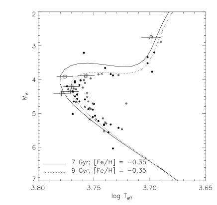
Figure 3: HR diagram for the stars that we followed up spectroscopically (solid symbols), and those from ST (crosses). Those in the tentative cluster identified in the bottom panel of Fig. 2 are indicated with larger light grey symbols with error bars. Stars with [Fe/H] $>-0.4$ dex are shown in dark grey. The temperature error bars correspond to $\pm 100$ K. The curves plotted are Yonsei-Yale isochrones (Demarque et al., 2004) with ${\rm[Fe/H]}=-0.35$ and ${\rm[\alpha/Fe]}=0.2$.

The bottom panel of Figure 2 shows ${\rm[\alpha/Fe]}$ vs ${\rm[Fe/H]}$ for the stars in our sample, where the black solid symbols indicate those that we have followed up and the crosses are from ST. We have highlighted with open symbols a set of 6 stars with ${\rm[Fe/H]}\sim-0.35$ dex. Closer examination of these stars reveals that 3 of them define a very cold kinematic group (visible in Fig. 1 at $V\sim-15$ and $U\sim-100$ km/s , + symbols). These stars’ eccentricities are 0.28, 0.31 and 0.32 while their ${\rm[Fe/H]}=-0.36$, $-0.26$, and $-0.33$ dex. The $\epsilon$ and ${\rm[Fe/H]}$ of the remaining 3 stars are also similar as shown in the central panel of Figure 2. This is also true for the chemical abundances of these stars (Fig. 4 below), for all measured elements except for [Mg/Fe] (where even those stars in the kinematic group depict a larger spread).

There are two possible interpretations that we may put forward: $i$) that the other 3 stars with similar ${\rm[Fe/H]}$ are a random sample of the thin disk, whose orbits are slightly hotter than typical for this component; $ii$) that they are part of the “kinematic clump” of 3 stars (a disrupted cluster?) because they are not very different dynamically, they have similar ${\rm[Fe/H]}$ and other abundances, as well as being indistinguishable in age (and clearly younger than the upper ${\rm[\alpha/Fe]}$ sequence at this metallicity). This is evident from Figure 3, where we plot the HR diagram of the stars in our sample. The lines correspond to 7 (solid) and 9 (dotted) Gyr old Yonsei-Yale isochrones (Demarque et al., 2004) with ${\rm[Fe/H]}=-0.35$ and ${\rm[\alpha/Fe]}=0.2$. We have also used a lighter gray colour for the stars with ${\rm[Fe/H]}>-0.4$ dex but higher ${\rm[\alpha/Fe]}$. This allows comparing the age of the stars in the tentative cluster to those stars with similar metallicity and eccentricity. Clearly those “cluster” stars are on average younger (as they have bluer colours, higher temperatures), and consistent with being a single age population. This motivates us to have a slight preference for the “cluster” scenario as it is not easy to understand why the contamination from the thin disk (which could be present for eccentricities $\sim 0.3$) would preferentially select stars with such a narrow range of ${\rm[Fe/H]}$. Our sample has no bias against stars with high metallicities, so one would perhaps have expected contaminants from a broader range of ${\rm[Fe/H]}$ more representative of the whole of the thin disk.

In summary, the bottom panel of Figure 2 shows that at high ${\rm[Fe/H]}$, stars define a narrow sequence depicting a steep relation between ${\rm[\alpha/Fe]}$ and ${\rm[Fe/H]}$, and that a transition occurs at ${\rm[Fe/H]}\sim-0.4$ dex, below which the scatter in ${\rm[\alpha/Fe]}$ increases significantly. Therefore the joint analysis of the panels in Fig. 2 suggests that at least two, but likely three, populations co-exist in our dataset: a low eccentricity population that dominates at high ${\rm[Fe/H]}$, a high eccentricity population that is essentially only present at low ${\rm[Fe/H]}$, and possibly a disrupted cluster. Note that none of these first two populations could belong to the thin disk given their kinematics and abundance trends. This is in agreement with the recent analysis of the Gaia-ESO survey by Recio-Blanco et al. (2014) that also shows a dearth of stars with high eccentricities at high ${\rm[Fe/H]}$ in the thick disk.

Figure 4 shows various element ratios as function of ${\rm[Fe/H]}$ for all the stars in our sample. We have used the same symbol scheme as in the bottom panel of Fig. 2, while the colour coding (from dark to light) and symbol size (from small to large) indicate increasing values of the eccentricity. The error bars correspond to two different estimates of our measurement uncertainties: from repeat observations of the same star (smaller bar) and from a global estimate (larger bar) derived from the change in the abundance of a given element as $T_{\rm eff}$ varies by $\sim\pm 100$ K, log $g$ by $\pm 0.1$ and ${\rm[Fe/H]}$ by $\pm 0.1$. The black points in the panels correspond to stars from Reddy et al. (2003, 2006) that have $\epsilon<0.3$ or $\epsilon>0.5$ (to provide a comparison sample with different kinematical characteristics from the H06 set). To be on the same scale, and using 15 stars we have in common, we applied a zero-point correction $\Delta={\rm[El/H]}_{us}-{\rm[El/H]}_{Reddy}$ to these abundances, namely $\Delta{\rm[Fe/H]}=0.09$, $\Delta{\rm[Mg/Fe]}=0.06$, $\Delta{\rm[Ca/Fe]}=0.08$, $\Delta{\rm[Ti/Fe]}=0.01$, $\Delta{\rm[Zn/Fe]}=0.02$, $\Delta{\rm[Cr/Fe]}=-0.03$ and $\Delta{\rm[Ni/Fe]}=-0.03$ (for more details, see Williams, 2008). The stars in ST have been put first on the Reddy scale, and later shifted in the same way. The dashed lines in the [Mg/Fe] vs ${\rm[Fe/H]}$ panel correspond to the sequences for the thin and thick disks as determined by Fuhrmann (2011) in his volume complete sample of nearby stars.

The three top left panels of this figure show that stars with ${\rm[Fe/H]}>-0.4$ define a relatively narrow track in [Mg/Fe], [Ca/Fe] and [Ti/Fe], with an internal dispersion smaller than the global estimated error, or even than the error determined from repeats. Note also that [Zn/Fe] and, even [Ni/Fe] follow clearly distinct tracks as function of ${\rm[Fe/H]}$, despite the fact that both Zn and Ni are Fe-peak elements. Recall that in this region of chemical space, most stars have lower eccentricities (darker symbols). We see once more that a transition in the chemical properties of the stars appears to occur at ${\rm[Fe/H]}\sim-0.4$, as the scatter substantially increases for all elements below this metallicity (also in ${\rm[SmII/Fe]}$, which is reasonable if this is largely an $r$-process product of massive stars, Mishenina et al., 2013). Also interesting is that the sequence delineated by the stars with ${\rm[Fe/H]}>-0.4$ appears to define an upper envelope at lower ${\rm[Fe/H]}$ (as there is a tendency for the darker symbols to have higher ${\rm[\alpha/Fe]}$ at these lower metallicities, and perhaps also lower [SmII/Fe]). The higher eccentricity and more metal-poor stars (lighter colours and larger symbols) follow well the sequence of “thick” disk stars, and given their kinematics, could be part of the canonical thick disk (as suggested by e.g. the uppermost dashed line in the [Mg/Fe] vs ${\rm[Fe/H]}$ panel).

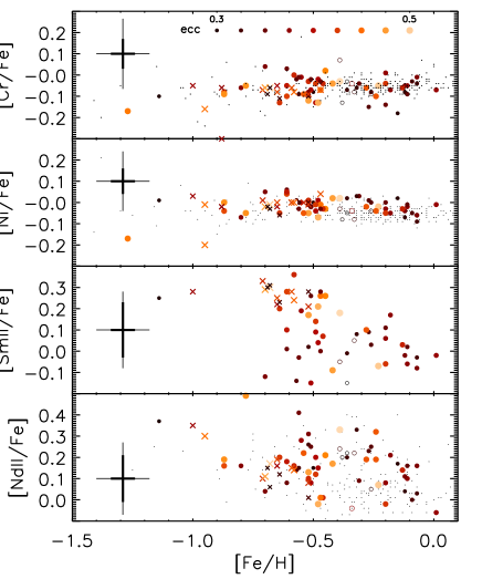
Figure 4: Various elements vs ${\rm[Fe/H]}$ for our sample of H06 stars (circles, where open symbols are for the tentative cluster) and for ST (crosses). The colour-coding (dark to light) and symbol size (small to large) indicates increasing eccentricity as shown in the top right. For comparison, we have also plotted (small dots) stars with $\epsilon<0.3$ and $\epsilon>0.5$ in the thin and thick disks from Reddy et al. (2003, 2006). The error bars indicate two estimates of our uncertainties: from repeats and from varying the derived astrophysical parameters.

Therefore the stars with lower $\epsilon$ tend to define the upper envelope of the ${\rm[\alpha/Fe]}$ vs. ${\rm[Fe/H]}$ both in our joint sample as well as in Reddy’s. It is also interesting to note that the highest ${\rm[Fe/H]}$ stars have lower [Zn/Fe], [Ti/Fe] than even the thin disk stars at this metallicity. On the other hand, their [Ca/Fe] is similar while their [Mg/Fe] is higher even than the thick disk stars at these ${\rm[Fe/H]}$.

The stars indicated with open symbols define very tight structures in [Ni/Fe] and also in [Ti/Fe]. In the other elements the scatter is consistent with the estimated global error. We may thus tentatively conclude that the indication of a single age (Fig. 3), their location in abundance space (which overlaps generally with thin disk stars), and their tight kinematics all are consistent with a (star) cluster origin for these stars.

The two stars with ${\rm[Fe/H]}\sim-0.87$ (HD 25704 and HD 63598) are particularly intriguing, since they have nearly identical compositions in all elements. They also share the same location in the HR diagram, implying that they have the same age (also confirmed by Casagrande et al., 2011). Furthermore, their distances are essentially identical ($\sim 50$ pc). According to their kinematics, they would be on relatively eccentric orbits, with $\epsilon=0.43$ and $0.47$ and velocities ($U$, $V$, $W$) = ($-127$, $-67$, $-9$) km/s and ($16$, $-108$, $1$) km/s, with average errors of 3 and 2 km/s respectively. A possibility is that these stars constitute a binary, as their velocity difference is too large for them to be located on the same orbital phase of a tidal stream.

3 Discussion

We have shown that stars with $0.3\leq\epsilon\leq 0.5$ do not form a homogeneous population. In this eccentricity range, a few populations with different characteristics are found:

• High metallicity stars (${\rm[Fe/H]}>-0.4$ dex) predominantly have lower eccentricities ($\epsilon\leq 0.4$), cold vertical kinematics, are ${\rm[\alpha/Fe]}$ enhanced, and define a relatively narrow track in all $\alpha$-elements vs ${\rm[Fe/H]}$, as well as in Zn and Ni. While their kinematics might suggest they could constitute the tail of the thin disk population, their abundances clearly rule out this possibility. This population is dominated by stars with an average age of 8 Gyr, and has no stars older than 12 Gyr.

• Lower metallicity stars can be on high or low eccentricity orbits, and show a larger abundance scatter than the population described in the previous item, and are also on average older, i.e. $\sim 9$ Gyr, with several stars as old as 14 Gyr. The higher eccentricity stars could be considered representative of the canonical thick disk.

• The third group of stars present in our dataset have very similar iron-peak abundances, and a somewhat larger scatter in $\alpha$ elements, especially in [Mg/Fe]. Half of these stars are also kinematically clustered in a tight clump, and all have similarly low eccentricities and ages, suggesting that they form a dynamical entity with a scale perhaps similar to that of a (star) cluster.

It is interesting to note that the first population overlaps with the high $\alpha$ metal-rich population in Adibekyan et al. (2013) (who also miss high-eccentricity metal-rich stars, see their Fig. 5). However in our sample, as in Bensby et al. (2013), there is no gap in ${\rm[Fe/H]}$ between this population and the more metal-poor stars.

The issue now is how to interpret these two main populations (i.e. excluding the tentative cluster) in the context of the evolution of our Galaxy. Let us consider the following possibilities.

• Mergers: In the most widely discussed scenario for the formation of the thick disk, a pre-existing disk is heated up via a minor merger. Such a disk would be more massive and hence have a higher metallicity, and lower eccentricity than the accreted population (Sales et al., 2009). Thus we would be tempted to identify this population with the sequence defined by the more metal-rich stars in our dataset, and the intruder with the higher eccentricity and lower ${\rm[Fe/H]}$ stars. The colder kinematics of the first group, ages and enhanced ${\rm[\alpha/Fe]}$ (i.e. higher SFR indicating more massive) would also seem to support this view.

• Canonical thick disk and bulge: Stars with higher eccentricities could be associated to the canonical thick disk, while those more metal-rich, could on the basis of their abundance patterns and ages be the extension of the bulge to the Solar neighbourhood. If this scenario is enforced, it would seem to be necessary to argue that the bulge/bar stars eccentricities and vertical motions are on average lower than those of the canonical thick disk, which appears slightly counterintuitive given our knowledge of in-situ bulge stars (e.g. Soto et al., 2012).

• Radial migration: In this scenario the high metallicity population would originate from the inner galactic disk (Grenon, 1999; Schoenrich & Binney, 2009). Hence one might expect such stars to have higher eccentricities (although migrated stars can also be on nearly circular orbits) as well as hotter $\sigma_{z}$ on average as postulated by Schoenrich & Binney (2009) (although see Minchev et al., 2012, who argue that if the vertical action is conserved, then the stars migrating from the inner disk become colder). On the other hand, the population of low ${\rm[Fe/H]}$ could not be considered the migrated population from the outer disk (as in the model by Haywood, 2008), because its $\sigma_{z}$ is higher than that of the thin disk locally, contrary to the prediction from simulations including radial migration (e.g. Solway et al., 2012; Minchev et al., 2012).

Which of these three scenarios is more likely is unclear, although the last one appears less plausible at face value in accounting for all the features observed.

It is interesting that we have not found that stars cluster in tight lumps at a fixed metallicity, except in a few occasions. Rather we have found sequences as expected for populations that have had a finite time to evolve (and self-enrich). The chemical evolution tracks are probably indicative of fairly intense star formation histories rather unlike those of e.g. dSph.

Our work suggests that the Milky Way’s disc(s) are the overlap of several populations with distinct characteristics. The combination of dynamics, stellar population analysis and chemical abundances have allowed us to establish this. However, we seem to be still a long way away from being able to deconstruct and understand the history of the Milky Way.

References

- Abadi et al. (2003) Abadi, M. G., Navarro, J. F., Steinmetz, M. & Eke, V. R. 2003, ApJ, 591, 499
- Adibekyan et al. (2013) Adibekyan, V. Z., Figueira, P., Santos, N. C., et al. 2013, A&A, 554, A44
- Arifyanto & Fuchs (2006) Arifyanto, M. I., & Fuchs, B. 2006, A&A, 449, 533
- Arlandini et al. (1999) Arlandini, C., Käppeler, F., Wisshak, K., Gallino, R., Lugaro, M., Busso, M. & Straniero, O. 1999, ApJ, 525, 886
- Belokurov et al. (2006) Belokurov, V., et al. 2006, ApJ, 642, L137
- Bensby et al. (2003) Bensby, T., Feltzing, S., and Lundström, I. 2003, A&A, 410, 527
- Bensby et al. (2005) Bensby, T., Feltzing, S., Lundström, I., and Ilyin, I. 2005, A&A, 433, 185
- Bensby et al. (2013) Bensby, T., Feltzing, S., & Oey, M. S. 2013, arXiv:1309.2631
- Bullock & Johnston (2005) Bullock, J. S. & Johnston, K. V. 2005, ApJ, 635, 931
- Burris et al. (2000) Burris, D. L., Pilachowski, C. A., Armandroff, T. E., Sneden, C., Cowan, J. J., and Roe, H. 2000, ApJ, 544, 302
- Casagrande et al. (2011) Casagrande, L., Schönrich, R., Asplund, M., et al. 2011, A&A, 530, A138
- De Silva et al. (2007) De Silva G. M., Freeman K. C., Bland-Hawthorn J., Asplund M., and Bessell M. S. 2007, AJ, 133, 694
- Demarque et al. (2004) Demarque P., Woo J.H., Kim Y.C., Yi S., 2004, ApJS, 155, 667
- Freeman & Bland-Hawthorn (2002) Freeman K. C. & Bland-Hawthorn J., 2002, ARA&A, 40, 487
- Fuhrmann (2011) Fuhrmann, K. 2011, MNRAS, 414, 2893
- Gilmore et al. (2002) Gilmore, G., Wyse, R. F. G., & Norris, J. E. 2002, ApJ, 574, L39
- Grenon (1999) Grenon, M. 1999, Ap&SS, 265, 331
- Haywood (2008) Haywood, M. 2008, MNRAS, 388, 1175
- Helmi & White (1999) Helmi, A. & White, S. D. M. 1999, MNRAS, 307, 495
- Helmi et al. (1999) Helmi, A., White, S. D. M., de Zeeuw, P. T. & Zhao, H. 1999, Nature, 402, 53
- Helmi et al. (2006) Helmi, A., et al. 2006, MNRAS, 365, 1309
- Holmberg et al. (2009) Holmberg, J., Nordström, B., & Andersen, J. 2009, A&A, 501, 941
- Majewski et al. (2012) Majewski, S. R., Nidever, D. L., Smith, V. V., et al. 2012, ApJ, 747, L37
- Meza et al. (2005) Meza, A., Navarro, J. F., Abadi, M. G., & Steinmetz, M. 2005, MNRAS, 359, 93
- Minchev et al. (2012) Minchev, I., Famaey, B., Quillen, A. C., et al. 2012, A&A, 548, A127
- Mishenina et al. (2013) Mishenina, T. V., Pignatari, M., Korotin, S. A., et al. 2013, A&A, 552, A128
- Navarro et al. (2004) Navarro, J. F., Helmi, A., & Freeman, K. C. 2004, ApJ, 601, L43
- Newberg et al. (2002) Newberg, H. J., et al. 2002, ApJ, 569, 245
- Nissen & Schuster (2011) Nissen, P. E., & Schuster, W. J. 2011, A&A, 530, A15
- Nissen & Schuster (2010) Nissen, P. E., & Schuster, W. J. 2010, A&A, 511, L10
- Nordström et al. (2004) Nordström, B., et al. 2004, A&A, 418, 989
- Recio-Blanco et al. (2014) Recio-Blanco, A., de Laverny, P., Kordopatis, G., et al. 2014, arXiv:1403.7568
- Reddy et al. (2003) Reddy, B. E., Tomkin, J., Lambert, D. L., and Allende Prieto, C. 2003, MNRAS, 340, 304
- Reddy et al. (2006) Reddy, B. E., Lambert, D. L., and Allende Prieto, C. 2006, MNRAS, 367, 1329
- Richardson et al. (2008) Richardson, J. C., et al. 2008, AJ, 135, 1998
- Sales et al. (2009) Sales, L.V. et al. 2009,MNRAS, 400, L61
- Schoenrich & Binney (2009) Schönrich, R., & Binney, J. 2009, MNRAS, 399, 1145
- Sneden (1973) Sneden, C. 1973, PhD thesis, University of Texas, Austin
- Solway et al. (2012) Solway, M., Sellwood, J. A., & Schönrich, R. 2012, MNRAS, 422, 1363
- Soto et al. (2012) Soto, M., Kuijken, K., & Rich, R. M. 2012, A&A, 540, A48
- Stetson & Pancino (2008) Stetson, P. B., & Pancino, E. 2008, PASP, 120, 1332
- Stonkutė et al. (2012) Stonkutė, E., Tautvaišienė, G., Nordström, B., & Ženovienė, R. 2012, A&A, 541, A157
- Stonkutė et al. (2013) Stonkutė, E., Tautvaišienė, G., Nordström, B., & Ženovienė, R. 2013, A&A, 555, A6
- Williams (2008) Williams, M. E. K., 2008, Australian National University
- Wylie-de Boer et al. (2010) Wylie-de Boer, E., Freeman, K., & Williams, M. 2010, AJ, 139, 636
- Wylie-de Boer et al. (2012) Wylie-de Boer, E., Freeman, K., Williams, M., et al. 2012, ApJ, 755, 35