The exponent in the orthogonality catastrophe
for Fermi gases

Abstract.

We quantify the asymptotic vanishing of the ground-state overlap of two non-interacting Fermi gases in $d$-dimensional Euclidean space in the thermodynamic limit. Given two one-particle Schrödinger operators in finite-volume which differ by a compactly supported bounded potential, we prove a power-law upper bound on the ground-state overlap of the corresponding non-interacting $N$-particle systems. We interpret the decay exponent $\gamma$ in terms of scattering theory and find $\gamma=\pi^{-2}\|\arcsin|T_{E}/2|\|_{\mathrm{HS}}^{2}$, where $T_{E}$ is the transition matrix at the Fermi energy $E$. This exponent reduces to the one predicted by Anderson [Phys. Rev. 164, 352–359 (1967)] for the exact asymptotics in the special case of a repulsive point-like perturbation.

1. Introduction

We consider two quantum systems, each consisting of $N$ non-interacting Fermions in a box of side length $L$ in $d$-dimensional Euclidean space $\mathbb{R}^{d}$, with $d\in\mathbb{N}$. The single-particle Hamiltonians of the two systems differ by a local perturbation potential $V$. As a signature of inequivalent representations of the canonical commutation relations, the overlap $\boldsymbol{\langle}\Phi^{N}_{L},\Psi^{N}_{L}\boldsymbol{\rangle}$ of the $N$-Fermion ground states $\Phi^{N}_{L}$ and $\Psi^{N}_{L}$ must vanish in the thermodynamic limit $L\to\infty$, $N\to\infty$, $N/L^{d}\to\text{const.}>0$ [Fri53, Chap. IV], [Haa96, Chap. II.1.1]. A quantitative version of this behaviour in terms of a power law

$$\bigl{\lvert}\boldsymbol{\langle}\Phi^{N}_{L},\Psi^{N}_{L}\boldsymbol{\rangle}\bigr{\rvert}^{2}\sim L^{-\gamma}$$ (1.1)

was predicted by P. W. Anderson in 1967. In [And67a] he presented a brief computation for the case of a point-like perturbation $V$ in $d=3$ dimensions and arrived at the upper bound

$$\bigl{\lvert}\boldsymbol{\langle}\Phi^{N}_{L},\Psi^{N}_{L}\boldsymbol{\rangle}\bigr{\rvert}^{2}\leqslant L^{-\gamma_{1}}$$ (1.2)

with

$$\gamma_{1}=\pi^{-2}(\sin\delta)^{2}.$$ (1.3)

Here, $\delta$ is the (single-particle) scattering phase shift caused by the point interaction at the Fermi energy. Nowadays, this behaviour is often referred to as Anderson’s orthogonality catastrophe in the physics literature. A mathematical proof for a generalisation of (1.2) and (1.3) was given recently in [GKM14]. Allowing for a bounded, compactly supported, non-negative perturbation $V$ in $\mathbb{R}^{d}$, it is shown there that (1.2) holds with

$$\gamma_{1}=\frac{1}{\pi^{2}}\,\lVert T_{E}/2\rVert_{\mathrm{HS}}^{2},$$ (1.4)

where $T_{E}$ denotes the transition matrix of scattering theory and $\lVert\,\boldsymbol{\cdot}\,\rVert_{\mathrm{HS}}$ the Hilbert-Schmidt norm for operators on the Hilbert space of the energy shell corresponding to the Fermi energy $E$. In the special case considered in [And67a], (1.4) reduces to (1.3). The principal strategy of the argument in [GKM14] is to rewrite the overlap determinant as $\lvert\boldsymbol{\langle}\Phi^{N}_{L},\Psi^{N}_{L}\boldsymbol{\rangle}\rvert^{2}=\det A=\exp(\operatorname{tr}\ln A)$ and to expand the logarithm in a series of non-negative terms

$$\bigl{\lvert}\boldsymbol{\langle}\Phi^{N}_{L},\Psi^{N}_{L}\boldsymbol{\rangle}\bigr{\rvert}^{2}=\exp\bigg{\{}-\sum_{n\in\mathbb{N}}\frac{1}{n}\,\operatorname{tr}\bigl{(}(I-A)^{n}\bigr{)}\bigg{\}},$$ (1.5)

see Lemma 3.1 below. A similar idea was used by M. Kac [Kac54] in his proof of the Szegő limit theorem for Toeplitz determinants which is, in a way, an analogue to (1.1).

By dropping all but the first term $\operatorname{tr}(I-A)$ of the series, which is called Anderson integral in the physics literature, one arrives at an upper bound. The main work of [GKM14] consists in deriving a lower bound of the form $\operatorname{tr}(I-A)\geqslant\gamma_{1}\ln L$ for the Anderson integral with $\gamma_{1}$ given by (1.4). There are only few other mathematically rigorous works on Anderson’s orthogonality catastrophe [KüOS14, G15a, KnOS15, G15b]. It is shown in [KüOS14] that (1.4) in fact provides the exact coefficient in the asymptotics $\operatorname{tr}(I-A)\sim\gamma_{1}\ln L$ of the Anderson integral in the thermodynamic limit for one-dimensional systems. We refer to [KüOS14, GKM14] and references therein for a brief description of the relevance of the orthogonality catastrophe in physics and for a discussion of the theoretical approaches in the physics literature.

In a second paper [And67b] in 1967, P. W. Anderson notes as an aside that the true asymptotics (1.1) of the overlap involves an exponent $\gamma$ for which “… the main difference from the previous result [i.e. (1.3)] is to replace $(\sin\delta)^{2}$ by $\delta^{2}$.” After some controversies about the correctness of interchanging limits [RS71, Ham71], Anderson’s result (1.1) was confirmed in the case of a point interaction $V$ with the decay exponent

$$\gamma=\pi^{-2}\delta^{2}$$ (1.6)

by theoretical-physics methods [Ham71]. A mathematical proof was given recently in [G15b]. For reasons of comparison, we remark that the particle number $N$ in [Ham71] refers to the number of $s$-orbital states below the Fermi energy and thus $N\sim L$. Related results in the context of the Kondo problem in the physics literature can be found in [NdD69, YA70].

The purpose of the present paper is a mathematical contribution towards the exact asymptotics (1.1). We will prove in Theorem 2.2 that, in the presence of a rather general background potential $V_{0}$, a bounded, compactly supported, non-negative perturbation potential $V$ in $\mathbb{R}^{d}$ causes the power-law decay

$$\bigl{\lvert}\boldsymbol{\langle}\Phi^{N}_{L},\Psi^{N}_{L}\boldsymbol{\rangle}\bigr{\rvert}^{2}\leqslant L^{-\gamma+\mathrm{o}(L^{0})}$$ (1.7)

of the overlap for almost every Fermi energy $E\in\mathbb{R}$ along subsequences $L\to\infty$. The decay exponent is given by

$$\gamma=\frac{1}{\pi^{2}}\bigl{\lVert}\arcsin\lvert T_{E}/2\rvert\bigr{\rVert}_{\mathrm{HS}}^{2}.$$ (1.8)

We refer to Theorem 2.2 for the precise statement. In proving (1.8), we obtain a result on the trace of a product of spectral projections of two Schrödinger operators which may be interesting by itself, see Theorem 3.4.

Clearly, when comparing (1.8) to (1.4), we infer $\gamma_{1}\leqslant\gamma$, and the two exponents are related in the spirit of Anderson’s rule quoted above. In view of [G15b] and of the physicists’ results, we conjecture that the exponent $\gamma$ governs the true asymptotics (1.1) of the overlap whenever the modulus of the (appropriately defined) scattering phases does not exceed $\pi/2$.

The proof of Theorem 2.2 relies on the representation (1.5) of the overlap. We determine the dominant behaviour of each term in the $n$-sum in (1.5), because each term contributes to the asymptotics. In order to treat the terms with $n>1$ we have to deal with additional issues. One is the non-positivity of certain trace expressions, another one is to compute the multi-dimensional integral

$$\int_{(0,\infty)^{2n}}\mathrm{d}u_{1}\dotsi\mathrm{d}u_{2n}\,\frac{e^{-(u_{1}+\dotsb+u_{2n})}}{(u_{1}+u_{2})\dotsm(u_{2n-1}+u_{2n})},$$ (1.9)

which contributes to the asymptotics of the $n$th term in (1.5). Subsequently, the values of these integrals show up in the Taylor expansion of the function $x\mapsto(\arcsin x)^{2}$. We compute the integral (1.9) in Sect. 4.5 by identifying it with the first diagonal matrix element of the $(2n-1)$th power of the Hilbert matrix.

Since $V$ causes scattering, the exponent $\gamma$ is typically expected to be strictly positive. In the appendix, we prove this in the case without a background potential.

After we completed this paper, Pushnitski and Frank [FP15] established results on the asymptotics for traces of regularised projections of infinite-volume operators. Their work is partly a generalisation of our analysis in Sections 4.3 to 4.5. In particular, their consequent use of Hankel operators is conceptually valuable and leads to a simplification of proofs. From this point of view it is also less surprising that (a unitary equivalent operator to) the Hilbert matrix appears in our Section 4.5 when we compute the multi-dimensional integral (1.9).

2. Setup and main result

Let $d\in\mathbb{N}$, $\Lambda_{1}\subseteq\mathbb{R}^{d}$ be open and bounded with $0\in\Lambda_{1}$ and for $L>1$, define $\Lambda_{L}:=L\cdot\Lambda_{1}$.

Let the negative Laplacian $-\Delta_{L}$ be supplied with Dirichlet boundary conditions on $\Lambda_{L}$. We define two multiplication operators $V_{0}$ and $V$ acting on $L^{2}(\Lambda_{L})$, corresponding to real-valued functions on $\mathbb{R}^{d}$ with the properties

$$\begin{gathered}\max\{V_{0},0\}\in K_{\mathrm{loc}}(\mathbb{R}^{d}),\quad\max\{-V_{0},0\}\in K(\mathbb{R}^{d}),\\ V\in L^{\infty}(\mathbb{R}^{d}),\quad V\geqslant 0,\quad\operatorname{supp}V\subseteq\Lambda_{1}\text{ compact.}\end{gathered}$$ (V)

Here, we have written $K(\mathbb{R}^{d})$ and $K_{\mathrm{loc}}(\mathbb{R}^{d})$ for the Kato class and the local Kato class, respectively, see [Sim82]. The finite-volume one-particle Schrödinger operators $H_{L}:=-\Delta_{L}+V_{0}$ and $H_{L}^{\prime}:=H_{L}+V$ are self-adjoint and densely defined in the Hilbert space $L^{2}(\Lambda_{L})$. The infinite-volume operators $H:=-\Delta+V_{0}$ and $H^{\prime}:=H+V$ are self-adjoint and densely defined in the Hilbert space $L^{2}(\mathbb{R}^{d})$. Birman’s theorem, see [BÈ67, Thm. 2] or [RS79, Thm. XI.10], is applicable by virtue of [Sim82, Thm. B.9.1] and guarantees the existence and completeness of the wave operators for the pair $H,H^{\prime}$. In particular, their absolutely continuous spectra are the same, i.e.

$$\sigma_{\mathrm{ac}}(H)=\sigma_{\mathrm{ac}}(H^{\prime}).$$ (2.1)

The assumptions (V) on $V_{0}$ and $V$, together with [BHL00, Thm. 6.1], imply that the semigroup operators $e^{-tH_{L}}$ and $e^{-tH_{L}^{\prime}}$ generated by the finite-volume one-particle operators $H_{L}$ and $H_{L}^{\prime}$ are trace class for every $t>0$, and, a fortiori, compact. In particular, $H_{L}$ and $H_{L}^{\prime}$ are bounded from below and have purely discrete spectra. We write $\lambda_{1}^{L}\leqslant\lambda_{2}^{L}\leqslant\dotsb$ and $\mu_{1}^{L}\leqslant\mu_{2}^{L}\leqslant\dotsb$ for their non-decreasing sequences of eigenvalues, counting multiplicities, and $(\varphi_{j}^{L})_{j\in\mathbb{N}}$ and $(\psi_{k}^{L})_{k\in\mathbb{N}}$ for the corresponding sequences of normalised eigenfunctions with an arbitrary choice of basis vectors in any eigenspace of dimension greater than one.

Given $N\in\mathbb{N}$, the induced (non-interacting) finite-volume $N$-particle Schrödinger operators $\hat{H}_{L}$ and $\hat{H}_{L}^{\prime}$ act on the totally antisymmetric subspace $\bigwedge_{j=1}^{N}L^{2}(\Lambda_{L})$ of the $N$-fold tensor product space and are given by

$$\hat{H}_{L}^{(\prime)}:=\sum_{j=1}^{N}I^{\,\otimes^{j-1}}\otimes H_{L}^{(\prime)}\otimes I^{\,\otimes^{N-j}}.$$ (2.2)

The corresponding ground states are given by the totally antisymmetrised products

$$\Phi^{N}_{L}:=\frac{1}{\sqrt{N!}}\,\varphi_{1}^{L}\wedge\dotsm\wedge\varphi_{N}^{L},\qquad\Psi^{N}_{L}:=\frac{1}{\sqrt{N!}}\,\psi_{1}^{L}\wedge\dotsm\wedge\psi_{N}^{L}.$$ (2.3)

In order to avoid ambiguities from possibly degenerate eigenspaces and to realise a given Fermi energy $E\in\mathbb{R}$ in the thermodynamic limit, we choose the number of particles as

$$N_{L}(E):=\#\{j\in\mathbb{N}:\,\lambda_{j}^{L}\leqslant E\}\in\mathbb{N}_{0},$$ (2.4)

which is the eigenvalue counting function of $H_{L}$ at $E$.

The quantity of interest is the ground-state overlap

$$\mathcal{S}_{L}(E):=\Bigl{\langle}\Phi_{L}^{N_{L}(E)},\Psi_{L}^{N_{L}(E)}\Bigr{\rangle}_{N_{L}{(E)}}=\det\Bigl{(}\langle\varphi_{j}^{L},\psi_{k}^{L}\rangle\Bigr{)}_{j,k=1,\dotsc,N_{L}(E)},$$ (2.5)

in particular its asymptotic behaviour as $L\to\infty$. In (2.5), $\langle\,\boldsymbol{\cdot}\,,\,\boldsymbol{\cdot}\,\rangle_{N}$ stands for the scalar product on the $N$-fermion space $\bigwedge_{j=1}^{N}L^{2}(\Lambda_{L})$, and $\langle\,\boldsymbol{\cdot}\,,\,\boldsymbol{\cdot}\,\rangle$ for the one on the single-particle space $L^{2}(\Lambda_{L})$. If $N_{L}(E)=0$, we set $\mathcal{S}_{L}(E):=1$.

Remark 2.1.

The particular choice (2.4) of $N_{L}(E)$ as an eigenvalue counting function turns out to be technically useful when conducting the thermodynamic limit, see Lemma 3.3 below. The particle density $\rho(E)$ of the two non-interacting fermion systems in the thermodynamic limit coincides with the integrated density of states

$$\rho(E)=\lim_{L\to\infty}\frac{N_{L}(E)}{L^{d}\,\lvert\Lambda_{1}\rvert}$$ (2.6)

of the single-particle Schrödinger operator $H$ (which is the same as the integrated density of states of $H^{\prime}$), provided the limit exists. Here, $\lvert\Lambda_{1}\rvert$ denotes the Lebesgue measure of $\Lambda_{1}\subseteq\mathbb{R}^{d}$. Situations where the limit (2.6) is known to exist include periodic $V_{0}$, or $V_{0}$ vanishing at infinity. If the limit (2.6) does not exist, then this is due to the occurrence of more than one accumulation point, because the assumptions on $V_{0}$ in (V), together with [Sim82, Thm. C.7.3], imply $\limsup_{L\to\infty}N_{L}(E)/L^{d}<\infty$ for every $E\in\mathbb{R}$. We will study the asymptotic behaviour of the overlap $\mathcal{S}_{L}(E)$ as $L\to\infty$ regardless of the existence of the limit (2.6).

The main result of this paper is an upper bound on the ground-state overlap $\mathcal{S}_{L}(E)$ for large $L$. Throughout we use the convention $\ln 0:=-\infty$. The terms null set and almost-every (a.e.) refer to Lebesgue measure if not specified otherwise.

Theorem 2.2 (Orthogonality Catastrophe).

Assume conditions (V). Let $(L_{m})_{m\in\mathbb{N}}$ be a sequence in $(0,\infty)$ with $L_{m}\to\infty$. Then there exist a subsequence $(L_{m_{k}})_{k\in\mathbb{N}}$, a null set $\mathcal{N}\subseteq\mathbb{R}$ of exceptional Fermi energies and a function $\gamma\colon\mathbb{R}\setminus\mathcal{N}\to[0,\infty)$ such that for every $E\in\mathbb{R}\setminus\mathcal{N}$ the ground-state overlap (2.5) obeys

$$\lvert\mathcal{S}_{L_{m_{k}}}(E)\rvert\leqslant\exp\Bigl{(}-\tfrac{1}{2}\gamma(E)\ln L_{m_{k}}+\mathrm{o}(\ln L_{m_{k}})\Bigr{)}=L_{m_{k}}^{-\gamma(E)/2+\mathrm{o}(1)}$$ (2.7)

as $k\to\infty$. Equivalently,

$$\limsup_{k\to\infty}\frac{\ln\lvert\mathcal{S}_{L_{m_{k}}}(E)\rvert}{\ln L_{m_{k}}}\leqslant-\frac{\gamma(E)}{2}.$$ (2.8)

The decay exponent $\gamma$ is given by

$$\gamma(E):=\frac{1}{\pi^{2}}\bigl{\lVert}\arcsin\lvert T_{E}/2\rvert\bigr{\rVert}_{\mathrm{HS}}^{2}.$$ (2.9)

Here, $T_{E}:=S_{E}-I_{E}$ is the transition matrix, $S_{E}$ is the scattering matrix for the pair $(H,H^{\prime})$ and energy $E$, and $\lVert\,\boldsymbol{\cdot}\,\rVert_{\mathrm{HS}}$ denotes the Hilbert–Schmidt norm on the fibre Hilbert space $\mathcal{H}_{E}$, on which $T_{E}$ and $S_{E}$ are defined.

Remarks 2.3.

• We refer to Subsection 4.6 for a more precise definition of the scattering-theoretic quantities $T_{E}$ and $S_{E}$.

• In proving Theorem 2.2, we obtain a result on the asymptotics of the trace $\operatorname{tr}\bigl{\{}\bigl{(}1_{(-\infty,E]}(H_{L})1_{(E,\infty)}(H_{L}^{\prime})\bigr{)}^{n}\bigr{\}}$ as $L\to\infty$, which may be interesting by itself; see Theorem 3.4.

• The reason for passing to a subsequence $(L_{m_{k}})_{k\in\mathbb{N}}$ in Theorem 2.2 originates from Lemma 3.3 below. What stands behind it is the lack of known a.e.-bounds on the finite-volume spectral shift function for the pair of operators $H_{L},H_{L}^{\prime}$, which hold uniformly in the limit $L\to\infty$. This unfortunate fact has been noticed many times in the literature, see e.g. [HM10], and the pathological behaviour of the spectral shift function found in [Kir87] illustrates that this is a delicate issue. However, in certain special situations such a.e.-bounds are known, and our result can be strengthened. More precisely, we have

Theorem 2.2’.  Assume the situation of Theorem 2.2 with $d=1$, or replace the perturbation potential $V$ in Theorem 2.2 by a finite-rank operator $V=\sum_{\nu=1}^{n}\langle\phi_{\nu},\,\boldsymbol{\cdot}\,\rangle\,\phi_{\nu}$ with compactly supported $\phi_{\nu}\in L^{2}(\mathbb{R}^{d})$ for $\nu=1,\ldots,n$, or consider the lattice problem on $\mathbb{Z}^{d}$ corresponding to the situation in Theorem 2.2. Then the ground-state overlap (2.5) obeys

$$\lvert\mathcal{S}_{L}(E)\rvert\leqslant\exp\Bigl{(}-\tfrac{1}{2}\gamma(E)\ln L+\mathrm{o}(\ln L)\Bigr{)}=L^{-\gamma(E)/2+\mathrm{o}(1)}$$ (2.10)

for a.e. $E\in\mathbb{R}$ as $L\to\infty$. Equivalently,

$$\limsup_{L\to\infty}\frac{\ln\lvert\mathcal{S}_{L}(E)\rvert}{\ln L}\leqslant-\frac{\gamma(E)}{2}$$ (2.11)

for a.e. $E\in\mathbb{R}$.

Remarks 2.4.

• In [GKM14], similar statements to Theorem 2.2 and Theorem 2.2’ were proved, in particular, the bound

  $${}{}\limsup_{L\to\infty}\frac{\ln\lvert\mathcal{S}_{L}(E)\rvert}{\ln L}\leqslant-\frac{\gamma_{1}(E)}{2},$$ (2.12)

  with the exponent

  $${}{}\gamma_{1}(E)=\frac{1}{\pi^{2}}\bigl{\lVert}T_{E}/2\bigr{\rVert}_{\mathrm{HS}}^{2}.$$ (2.13)

  Note that $\gamma_{1}(E)$, which is called $\gamma(E)$ in [GKM14], is strictly smaller than $\gamma(E)$ whenever both are non-zero. The bigger exponent $\gamma(E)$ is due to treating all terms in a series expansion of $\ln\lvert\mathcal{S}_{L}(E)\rvert$ (see equation (3.2) below) instead of only the Anderson integral, which is the first term of the series and gives rise to $\gamma_{1}(E)$.

• Another mathematical work dealing with AOC is [KüOS14]. That paper proves the exact asymptotics of the Anderson integral in the special case $d=1$ and $V_{0}=0$. In particular, this yields a bound on the overlap as in (2.12) with the same non-optimal $\gamma_{1}(E)$ given by (2.13). The paper also provides a lower bound on $\mathcal{S}_{L}(E)$ with a smaller decay exponent [KüOS14, Cor. 5.6].

3. Series expansion of the overlap

In order to expand the ground-state overlap as a series, we introduce the orthogonal projections

$$P^{N}_{L}:=\sum_{j=1}^{N}\langle\varphi_{j}^{L},\,\boldsymbol{\cdot}\,\rangle\varphi_{j}^{L}\quad\text{and}\quad\Pi^{N}_{L}:=\sum_{k=1}^{N}\langle\psi_{k}^{L},\,\boldsymbol{\cdot}\,\rangle\psi_{k}^{L}$$ (3.1)

for $N\in\mathbb{N}_{0}$, i.e. the projections on the eigenspaces of the first $N$ eigenvalues. Using those, we can prove the following lemma.

Lemma 3.1.

Let $L>1$, $E\in\mathbb{R}$ and assume that $\mathcal{S}_{L}(E)\neq 0$. Then

$$\lvert\mathcal{S}_{L}(E)\rvert^{2}=\exp\biggl{(}-\sum_{n=1}^{\infty}\frac{1}{n}\operatorname{tr}\Bigl{\{}\Bigl{(}P^{N_{L}(E)}_{L}\bigl{(}I-\Pi^{N_{L}(E)}_{L}\bigr{)}\Bigr{)}^{n}\Bigr{\}}\biggr{)},$$ (3.2)

where we take the trace of operators on the Hilbert space $L^{2}(\Lambda_{L})$.

• For brevity, set $N:=N_{L}(E)$. If $N=0$, the assertion is true by definition. Otherwise, define the $N\times N$-matrix $M:=\bigl{(}\langle\varphi_{j}^{L},\psi_{k}^{L}\rangle\bigr{)}_{j,k=1,\dotsc,N}$. Then $\mathcal{S}_{L}(E)=\det M$ and $\lvert\mathcal{S}_{L}(E)\rvert^{2}=\det({MM}^{*})$. For $1\leqslant j,\ell\leqslant N$, the $(j,\ell)$-th entry of ${MM}^{*}$ is

  $$(MM^{*})_{j,\ell}=\sum_{k=1}^{N}\langle\varphi_{j}^{L},\psi_{k}^{L}\rangle\langle\psi_{k}^{L},\varphi_{\ell}^{L}\rangle=\langle\varphi_{j}^{L},\Pi_{L}^{N}\varphi_{\ell}^{L}\rangle=\langle\varphi_{j}^{L},P_{L}^{N}\Pi_{L}^{N}P_{L}^{N}\varphi_{\ell}^{L}\rangle.$$ (3.3)

  Since $\mathcal{S}_{L}(E)\neq 0$ by assumption and therefore ${MM}^{*}>0$, we have $0\leq P_{L}^{N}(I-\Pi_{L}^{N})P_{L}^{N}<1$. Moreover, being of finite rank, $P_{L}^{N}(I-\Pi_{L}^{N})P_{L}^{N}$ is a trace class operator. Thus, we compute

  $$\lvert\mathcal{S}_{L}(E)\rvert^{2} =\det\left(I-P_{L}^{N}(I-\Pi_{L}^{N})P_{L}^{N}\right)$$

  $$=\exp\Bigl{(}\operatorname{tr}\Bigl{\{}\ln\bigl{(}I-P_{L}^{N}(I-\Pi_{L}^{N})P_{L}^{N}\bigr{)}\Bigr{\}}\Bigr{)}$$

  $$=\exp\biggl{(}-\operatorname{tr}\biggl{\{}\sum_{n=1}^{\infty}\frac{1}{n}\Bigl{(}P_{L}^{N}(I-\Pi_{L}^{N})P_{L}^{N}\Bigr{)}^{n}\biggr{\}}\biggr{)}$$

  $$=\exp\biggl{(}-\sum_{n=1}^{\infty}\frac{1}{n}\operatorname{tr}\Bigl{\{}\Bigl{(}P_{L}^{N}(I-\Pi_{L}^{N})\Bigr{)}^{n}\Bigr{\}}\biggr{)},$$ (3.4)

  where we used the expansion $\ln(1-x)=-\sum_{n=1}^{\infty}x^{n}/n$ for the logarithm, which converges absolutely for $\lvert x\rvert<1$. ∎

Remark 3.2.

Lemma 3.1 will be the starting point of our estimates for $\lvert\mathcal{S}_{L}(E)\rvert$. Equation (3.2) can be written as

$$-\ln\lvert\mathcal{S}_{L}(E)\rvert=\frac{1}{2}\sum_{n=1}^{\infty}\frac{1}{n}\operatorname{tr}\Bigl{\{}\Bigl{(}P^{N_{L}(E)}_{L}(I-\Pi^{N_{L}(E)}_{L})\Bigr{)}^{n}\Bigr{\}}.$$ (3.5)

The trace expressions in (3.5) are non-negative, so any truncation of the series yields a lower bound on $-\ln\lvert\mathcal{S}_{L}(E)\rvert$, and therefore an upper bound on the overlap. Keeping only the term for $n=1$, one recovers the so-called Anderson integral, which was estimated in [GKM14].

In the sequel, we will find an upper bound on $\lvert\mathcal{S}_{L}(E)\rvert$ by bounding each individual term of (3.5) from below.

We begin by recasting the orthogonal projections (3.1) as functions of $H_{L}$ and $H_{L}^{\prime}$ in the sense of the spectral calculus. The projections in (3.1) are not necessarily functions of $H_{L}$ and $H_{L}^{\prime}$, since the $N$th eigenvalues might be of multiplicity higher than one. The choice of $N_{L}(E)$ in (2.4), together with a convergence result of the spectral shift function, allows us to rewrite them, at the cost of passing to a subsequence of lengths.

Lemma 3.3.

For $n\in\mathbb{N}$, $L>1$ and $E\in\mathbb{R}$, define

$$\mathcal{F}^{n}_{L}(E):=\operatorname{tr}\Bigl{\{}\Bigl{(}1_{(-\infty,E]}(H_{L})1_{(E,\infty)}(H_{L}^{\prime})\Bigr{)}^{n}\Bigr{\}}$$ (3.6)

and

$$\mathcal{I}^{n}_{L}(E):=\operatorname{tr}\Bigl{\{}\Bigl{(}P^{N_{L}(E)}_{L}(I-\Pi^{N_{L}(E)}_{L})\Bigr{)}^{n}\Bigr{\}}.$$ (3.7)

Then

• Assume (V) and let $(L_{m})_{m\in\mathbb{N}}\subset(0,\infty)$ be a sequence of increasing lengths with $L_{m}\uparrow\infty$. Then there exists a subsequence $(L_{m_{k}})_{k\in\mathbb{N}}$ such that for a.e. Fermi energy $E\in\mathbb{R}$

  $${}{}\bigl{\lvert}\mathcal{F}^{n}_{L_{m_{k}}}(E)-\mathcal{I}^{n}_{L_{m_{k}}}(E)\bigr{\rvert}=\mathrm{o}(\ln L_{m_{k}})$$ (3.8)

  as $k\to\infty$.

• Assume the situation of Theorem 2.2’. Then

  $$\sup_{L>1}\sup_{E\in\mathbb{R}}\bigl{\lvert}\mathcal{F}^{n}_{L}(E)-\mathcal{I}^{n}_{L}(E)\bigr{\rvert}<\infty.$$ (3.9)

• For fixed $L>1$ and $E\in\mathbb{R}$, the definition of $N_{L}(E)$ in $\eqref{eq:N}$ implies

  $$\lambda_{N_{L}(E)}^{L}\leqslant E<\lambda_{N_{L}(E)+1}^{L}\leqslant\mu_{N_{L}(E)+1}^{L}$$ (3.10)

  if we set $\lambda_{0}^{L}:=-\infty$. This allows us to write

  $$P_{L}^{N_{L}(E)}=1_{(-\infty,E]}(H_{L})$$ (3.11)

  and

  $$I-\Pi^{N_{L}(E)}_{L} =1_{(E,\infty)}(H_{L}^{\prime})-\sum_{k=1}^{N_{L}(E)}1_{(E,\infty)}(\mu_{k}^{L})\,\langle\psi_{k}^{L},\,\boldsymbol{\cdot}\,\rangle\psi_{k}^{L}$$

  $$=:1_{(E,\infty)}(H_{L}^{\prime})-Q.$$ (3.12)

  The operator $Q$ is an orthogonal projection with trace

  $$\operatorname{tr}Q =\#\bigl{\{}k\in\{1,\dotsc,N_{L}(E)\}:\,\mu_{k}^{L}>E\bigr{\}}$$

  $$=N_{L}(E)-\#\bigl{\{}k\in\mathbb{N}:\,\mu_{k}^{L}\leqslant E\bigr{\}}=:\xi_{L}(E)$$ (3.13)

  equal to the finite-volume spectral-shift function at the Fermi energy.

  Using $A^{n}-B^{n}=\sum_{k=1}^{n}B^{k-1}(A-B)A^{n-k}$ for bounded operators $A$ and $B$, we write the difference of operator powers on the left-hand side of (3.8) as

  $$\Bigl{(}P^{N_{L}(E)}_{L}1_{(E,\infty)}(H_{L}^{\prime})\Bigr{)}^{n}-\Bigl{(}P^{N_{L}(E)}_{L}(I-\Pi^{N_{L}(E)}_{L})\Bigr{)}^{n}\\ =\sum_{k=1}^{n}\Bigl{(}P^{N_{L}(E)}_{L}(I-\Pi^{N_{L}(E)}_{L})\Bigr{)}^{k-1}P^{N_{L}(E)}_{L}\,Q\,\Bigl{(}P^{N_{L}(E)}_{L}1_{(E,\infty)}(H_{L}^{\prime})\Bigr{)}^{n-k},$$ (3.14)

  where we also use (3.11). We estimate the traces of the operators on the right-hand side of (3.14) by bounding the operator norms of all projections, except for $Q$, by $1$. We then arrive at $n\xi_{L}(E)$ as a upper bound for (3.14). The claim follows by exploiting the weak convergence of $\xi_{L}$ as $L\to\infty$ [HM10, Thm. 1.4] in the situation of (i), or using the uniform boundedness of $\xi_{L}$ in the situation of (ii). We refer to [GKM14, Lemma 3.9] for a detailed argument. ∎

Having established (3.8), we will prove a diverging lower bound for $\operatorname{tr}\bigl{\{}\bigl{(}1_{(-\infty,E]}(H_{L})1_{(E,\infty)}(H_{L}^{\prime})\bigr{)}^{n}\bigr{\}}$ as $L\to\infty$. There will be no restriction to particular sequences of lengths from now on. The following theorem is the main ingredient of the proof.

Theorem 3.4.

Assume the situation of Theorem 2.2 or Theorem 2.2’. Then there exists a null set $\mathcal{N}\subset\mathbb{R}$ of exceptional Fermi energies such that

$$\operatorname{tr}\bigl{\{}\bigl{(}1_{(-\infty,E]}(H_{L})1_{(E,\infty)}(H_{L}^{\prime})\bigr{)}^{n}\bigr{\}}\geqslant nJ_{2n}\operatorname{tr}(\lvert T_{E}/(2\pi)\rvert^{2n})\ln L+\mathrm{o}(\ln L)$$ (3.15)

for every $E\in\mathbb{R}\setminus\mathcal{N}$ and every $n\in\mathbb{N}$ as $L\to\infty$. The error term $\mathrm{o}(\ln L)$ depends on $n$ and $E$, and we introduced the constant

$$J_{2n}:=\pi^{2(n-1)}2^{2n-1}\frac{[(n-1)!]^{2}}{(2n)!}.$$ (3.16)

Remarks 3.5.

• In the next section, we will spell out explicitly the proof of Theorem 3.4 for the situation of Theorem 2.2 only. It follows from Corollary 4.25, Theorem 4.26 and Theorem 4.32. The proof is fully analogous (and even simpler) in the remaining situations of Theorem 2.2’, where $V$ is a finite-rank operator.

• The constant $J_{2n}$ will emerge as the value of a $2n$-dimensional integral which we calculate using the spectral representation of the Hilbert matrix, see Subsection 4.5 below.

Given Theorem 3.4, we are now in a position to prove Theorem 2.2.

• Let $M\in\mathbb{N}$. Let $\mathcal{N}$ be the null set from Theorem 3.4. Let $E\in\mathbb{R}\setminus\mathcal{N}$. We start from Lemma 3.1 and Lemma 3.3, which imply

  $$-\ln\lvert\mathcal{S}_{L_{m_{k}}}(E)\rvert \geqslant\frac{1}{2}\sum_{n=1}^{M}\frac{1}{n}\operatorname{tr}\Bigl{\{}\Big{(}P^{N_{L_{m_{k}}}(E)}_{L_{m_{k}}}\big{(}I-\Pi^{N_{L_{m_{k}}}(E)}_{L_{m_{k}}}\big{)}\Big{)}^{n}\Bigr{\}}$$

  $$=\frac{1}{2}\sum_{n=1}^{M}\frac{1}{n}\operatorname{tr}\Bigl{\{}\Bigl{(}1_{(-\infty,E]}(H_{L_{m_{k}}})1_{(E,\infty)}(H_{L_{m_{k}}}^{\prime})\Bigr{)}^{n}\Bigr{\}}$$

  $$\quad+\mathrm{o}(\ln L_{m_{k}})$$ (3.17)

  for a subsequence $(L_{m_{k}})_{k\in\mathbb{N}}$, as $k\to\infty$, with an $M$-dependent error term $\mathrm{o}(\ln L_{m_{k}})$. By Theorem 3.4, this gives

  $$-\ln\lvert\mathcal{S}_{L_{m_{k}}}(E)\rvert\geqslant\frac{1}{2}\operatorname{tr}\sum_{n=1}^{M}J_{2n}\kern 0.41672pt\lvert T_{E}/(2\pi)\rvert^{2n}\ln L_{m_{k}}+\mathrm{o}(\ln L_{m_{k}})$$ (3.18)

  as $k\to\infty$, with an $M$-dependent error term $\mathrm{o}(\ln L_{m_{k}})$. The constants $J_{2n}$ show up in the series expansion [GR07, Eq. 1.645 2]

  $$\sum_{n=1}^{\infty}J_{2n}x^{2n}=\pi^{-2}\bigl{(}\arcsin(\pi x)\bigr{)}^{2}\qquad\text{for }\lvert x\rvert\leqslant\tfrac{1}{\pi}.$$ (3.19)

  Therefore, monotone convergence and the functional calculus yield

  $$\lim_{M\to\infty}\operatorname{tr}\sum_{n=1}^{M}J_{2n}\lvert T_{E}/(2\pi)\rvert^{2n}=\pi^{-2}\bigl{\lVert}\arcsin\lvert T_{E}/2\rvert\bigr{\rVert}_{\mathrm{HS}}^{2}.$$ (3.20)

  Since (3.18) is valid for every $M\in\mathbb{N}$, we infer

  $$\limsup_{k\to\infty}\frac{\ln\lvert\mathcal{S}_{L_{m_{k}}}(E)\rvert}{\ln L_{m_{k}}}\leqslant-\frac{1}{2}\pi^{-2}\bigl{\lVert}\arcsin\lvert T_{E}/2\rvert\bigr{\rVert}_{\mathrm{HS}}^{2}=-\frac{\gamma(E)}{2},$$ (3.21)

  which proves (2.8). For (2.7), note that by the definition of the limit superior for every $\varepsilon>0$ there is $k_{0}\in\mathbb{N}$ such that

  $$\frac{\ln\lvert\mathcal{S}_{L_{m_{k}}}(E)\rvert}{\ln L_{m_{k}}}\leqslant-\frac{\gamma(E)}{2}+\varepsilon$$ (3.22)

  for all $k\geq k_{0}$, which implies the claim. ∎

It remains to prove Theorem 3.4.

4. Proof of Theorem 3.4

4.1. An integral representation for $\operatorname{tr}\bigl{\{}\bigl{(}f(H_{L})g(H_{L}^{\prime})\bigr{)}^{n}\bigr{\}}$

Throughout this subsection, $n\in\mathbb{N}$, $L>1$ and $E\in\mathbb{R}$ are all fixed. Using the eigenvalue equations of $H_{L}$ and $H_{L}^{\prime}$, we rewrite trace expressions like (3.6).

Lemma 4.1.

Let $f,g\colon\mathbb{R}\to[0,1]$ be measureable functions with compact supports $\operatorname{supp}f\subseteq(-\infty,E]$ and $\operatorname{supp}g\subseteq(E,\infty)$. Then

$$\operatorname{tr}\bigl{\{}\bigl{(}f(H_{L})g(H_{L}^{\prime})\bigr{)}^{n}\bigr{\}}\\ =\sum_{\alpha,\beta\in\mathbb{N}^{n}}\prod_{j=1}^{n}\biggl{(}f(\lambda_{\alpha_{j}}^{L})g(\mu_{\beta_{j}}^{L})\frac{\langle\varphi_{\alpha_{j}}^{L},V\psi_{\beta_{j}}^{L}\rangle\langle\psi_{\beta_{j}}^{L},V\varphi_{\alpha_{j+1}}^{L}\rangle}{(\mu_{\beta_{j}}^{L}-\lambda_{\alpha_{j}}^{L})(\mu_{\beta_{j}}^{L}-\lambda_{\alpha_{j+1}}^{L})}\biggr{)},$$ (4.1)

for multi-indices $\alpha=(\alpha_{1},\dotsc,\alpha_{n})\in\mathbb{N}^{n}$ with the convention $\alpha_{n+1}:=\alpha_{1}$.

• We begin noting that

  $$f(H_{L})=\sum_{j\in\mathbb{N}}f(\lambda_{j}^{L})\,\langle\varphi_{j}^{L},\,\boldsymbol{\cdot}\,\rangle\varphi_{j}^{L},\qquad g(H_{L}^{\prime})=\sum_{k\in\mathbb{N}}g(\mu_{k}^{L})\,\langle\psi_{k}^{L},\,\boldsymbol{\cdot}\,\rangle\psi_{k}^{L}.$$ (4.2)

  To ease notation, we employ the bra-ket notation in the next formula, writing $\langle\varphi,\,\boldsymbol{\cdot}\,\rangle\varphi=:\lvert\kern 0.41672pt\varphi\rangle\langle\varphi\kern 0.41672pt\rvert$ for $\varphi\in L^{2}(\Lambda_{L})$. Then (4.2) implies

  $$\bigl{(}f(H_{L})g(H_{L}^{\prime})\bigr{)}^{n}=\sum_{\alpha,\beta\in\mathbb{N}^{n}}\Bigl{(}\prod_{j=1}^{n}f(\lambda_{\alpha_{j}}^{L})g(\mu_{\beta_{j}}^{L})\Bigr{)}\,\prod_{j=1}^{n}\lvert\kern 0.41672pt\varphi_{\alpha_{j}}^{L}\rangle\langle\varphi_{\alpha_{j}}^{L},\psi_{\beta_{j}}^{L}\rangle\langle\psi_{\beta_{j}}^{L}\kern 0.41672pt\rvert,$$ (4.3)

  and

  $$\operatorname{tr}\bigl{\{}\bigl{(}f(H_{L})g(H_{L}^{\prime})\bigr{)}^{n}\bigr{\}}\\ =\sum_{\alpha,\beta\in\mathbb{N}^{n}}\Bigl{(}\prod_{j=1}^{n}f(\lambda_{\alpha_{j}}^{L})g(\mu_{\beta_{j}}^{L})\Bigr{)}\,\prod_{j=1}^{n}\langle\varphi_{\alpha_{j}}^{L},\psi_{\beta_{j}}^{L}\rangle\langle\psi_{\beta_{j}}^{L},\varphi_{\alpha_{j+1}}^{L}\rangle,$$ (4.4)

  where we used the convention $\alpha_{n+1}:=\alpha_{1}$ for $\alpha\in\mathbb{N}^{n}$. Now, we note that the eigenvalue equations imply

  $$\lambda_{j}^{L}\langle\varphi_{j}^{L},\psi_{k}^{L}\rangle=\langle H_{L}\varphi_{j}^{L},\psi_{k}^{L}\rangle=\mu_{k}^{L}\langle\varphi_{j}^{L},\psi_{k}^{L}\rangle-\langle\varphi_{j}^{L},V\psi_{k}^{L}\rangle$$ (4.5)

  for $j,k\in\mathbb{N}$, and therefore

  $$\langle\varphi_{j}^{L},\psi_{k}^{L}\rangle=\frac{\langle\varphi_{j}^{L},V\psi_{k}^{L}\rangle}{\mu_{k}^{L}-\lambda_{j}^{L}}$$ (4.6)

  whenever $\lambda_{j}^{L}\neq\mu_{k}^{L}$. Since $f$ and $g$ have disjoint supports, (4.6) and (4.4) yield the claim. ∎

Remark 4.2.

In analogy to [GKM14], one might be tempted to define a spectral correlation “measure” by

$$\mu_{L}^{2n}(A_{1}\times\dotsm\times A_{n}\times B_{1}\times\dotsm\times B_{n})\\ :=\operatorname{tr}\big{\{}(1_{A_{1}}(H_{L})V1_{B_{1}}(H_{L}^{\prime})V\;\dotsm\;1_{A_{n}}(H_{L})V1_{B_{n}}(H_{L}^{\prime})V)\big{\}}$$ (4.7)

for $n\in\mathbb{N}$,  $L>1$ and bounded $A_{1},\dotsc,A_{n},B_{1},\dotsc,B_{n}\in\operatorname{Borel}(\mathbb{R})$, which was done for the case $n=1$ in [GKM14]. Lemma 4.1 would then read

$$\operatorname{tr}\bigl{\{}\bigl{(}f(H_{L})g(H_{L}^{\prime})\bigr{)}^{n}\bigr{\}}=\int_{\mathbb{R}^{n}\times\mathbb{R}^{n}}\mathrm{d}\mu_{L}^{2n}(x,y)\prod_{j=1}^{n}\frac{f(x_{j})g(y_{j})}{(y_{j}-x_{j})(y_{j}-x_{j+1})}.$$ (4.8)

However, (4.7) is not necessarily non-negative for $n\geqslant 2$, and therefore we cannot mimick the proof of [GKM14].

Next, we rewrite the right-hand side of (4.1) using a variation of an integral formula that goes back to Feynman and Schwinger.

Lemma 4.3 (Feynman–Schwinger parametrization).

Let $x_{1},\dotsc,x_{n}\in(0,\infty)$. Then

$$\frac{1}{x_{1}\dotsm x_{n}}=\int_{0}^{\infty}\mathrm{d}t\,t^{n-1}\int_{(0,\infty)^{n}}\mathrm{d}u\,\lvert u\rvert_{1}e^{-\lvert u\rvert_{1}}e^{-tu\cdot x},$$ (4.9)

where $u\cdot x=\sum_{j=1}^{n}u_{j}x_{j}$ denotes the Euclidean scalar product and $\lvert u\rvert_{1}:=\sum_{j=1}^{n}\lvert u_{j}\rvert$ the $1$-norm on $\mathbb{R}^{n}$.

• For any measurable function $f\colon(0,\infty)^{n}\to(0,\infty)$ the coarea formula implies

  $$\int_{(0,\infty)^{n}}\mathrm{d}u\,f(u)=\int_{0}^{\infty}\mathrm{d}t\int_{\mathcal{M}}\frac{\mathrm{d}S(\xi)}{\sqrt{n}}t^{n-1}f(t\xi),$$ (4.10)

  where $\mathrm{d}S$ stands for integration with respect to the surface measure on $\mathcal{M}:=\{\xi\in(0,\infty)^{n}:\,\lvert\xi\rvert_{1}=1\}$. Let $r>0$. Starting from $x_{j}^{-1}=\int_{0}^{\infty}\mathrm{d}u_{j}\,e^{-u_{j}x_{j}}$, we compute using (4.10)

  $$\frac{1}{x_{1}\dotsm x_{n}} =\int_{(0,\infty)^{n}}\mathrm{d}u\,e^{-u\cdot x}=\int_{0}^{\infty}\mathrm{d}t\int_{\mathcal{M}}\frac{\mathrm{d}S(\xi)}{\sqrt{n}}t^{n-1}e^{-t\xi\cdot x}$$

  $$=\int_{0}^{\infty}\mathrm{d}t\int_{\mathcal{M}}\frac{\mathrm{d}S(\xi)}{\sqrt{n}}t^{n-1}r^{n}e^{-rt\xi\cdot x},$$ (4.11)

  which is $r$-independent. Given any measurable function $g\colon(0,\infty)\to(0,\infty)$ with $\int_{0}^{\infty}\mathrm{d}r\,\frac{g(r)}{r}=1$, we therefore get

  $$\frac{1}{x_{1}\dotsm x_{n}} =\int_{0}^{\infty}\mathrm{d}r\,g(r)\int_{0}^{\infty}\mathrm{d}t\int_{\mathcal{M}}\frac{\mathrm{d}S(\xi)}{\sqrt{n}}t^{n-1}r^{n-1}e^{-rt\xi\cdot x}$$

  $$=\int_{0}^{\infty}\mathrm{d}t\,t^{n-1}\int_{(0,\infty)^{n}}\mathrm{d}u\,g(\lvert u\rvert_{1})e^{-tu\cdot x},$$ (4.12)

  where we used the Fubini–Tonelli theorem and (4.10) with $f(u)=g(\lvert u\rvert_{1})e^{-tu\cdot x}$. Choosing $g(r):=re^{-r}$ finishes the proof. ∎

We use (4.9) to rewrite the right-hand side of (4.1).

Lemma 4.4.

Let $f,g\colon\mathbb{R}\to[0,1]$ be measurable functions with compact supports $\operatorname{supp}f\subseteq(-\infty,E]$ and $\operatorname{supp}g\subseteq(E,\infty)$. Then,

$$\operatorname{tr}\bigl{\{}\bigl{(}f(H_{L})g(H_{L}^{\prime})\bigr{)}^{n}\bigr{\}}\\ \quad=\int_{0}^{\infty}\mathrm{d}t\,t^{2n-1}\int_{(0,\infty)^{n}\times(0,\infty)^{n}}\mathrm{d}(u,v)\,(\lvert u\rvert_{1}+\lvert v\rvert_{1})e^{-\lvert u\rvert_{1}-\lvert v\rvert_{1}}\hfill\\ \qquad\times\operatorname{tr}\bigg{\{}\prod_{j=1}^{n}\sqrt{V}f(H_{L})e^{(u_{j}+v_{j-1})t(H_{L}-E)}Vg(H_{L}^{\prime})e^{-(u_{j}+v_{j})t(H_{L}^{\prime}-E)}\sqrt{V}\bigg{\}}\hfill$$ (4.13)

with the convention $v_{0}:=v_{n}$ for $v\in\mathbb{R}^{n}$.

• Let $x\in(-\infty,0]^{n}$, $y\in(0,\infty)^{n}$ and define $x_{n+1}:=x_{1}$. Then, by (4.9),

  $$\frac{1}{\prod_{j=1}^{n}(y_{j}-x_{j})(y_{j}-x_{j+1})}\\ \qquad=\int_{0}^{\infty}\mathrm{d}t\,t^{2n-1}\int_{(0,\infty)^{n}\times(0,\infty)^{n}}\mathrm{d}(u,v)\,(\lvert u\rvert_{1}+\lvert v\rvert_{1})e^{-\lvert u\rvert_{1}-\lvert v\rvert_{1}}\\ \times\exp\biggl{(}-t\sum_{j=1}^{n}\big{(}u_{j}(y_{j}-x_{j})+v_{j}(y_{j}-x_{j+1})\big{)}\biggr{)}$$ (4.14)

  and

  $$\sum_{j=1}^{n}\big{(}u_{j}(y_{j}-x_{j})+v_{j}(y_{j}-x_{j+1})\big{)}=\sum_{j=1}^{n}\bigl{(}(u_{j}+v_{j})y_{j}-(u_{j}+v_{j-1})x_{j}\bigr{)}$$ (4.15)

  for $u,v\in(0,\infty)^{n}$. Now, let $\alpha,\beta\in\mathbb{N}^{n}$. Setting $x_{j}=\lambda_{\alpha_{j}}^{L}-E$ and $y_{j}=\mu_{\beta_{j}}^{L}-E$, we can write the denominator in (4.1) as

  $$\frac{1}{\prod_{j=1}^{n}(\mu_{\beta_{j}}^{L}-\lambda_{\alpha_{j}}^{L})(\mu_{\beta_{j}}^{L}-\lambda_{\alpha_{j+1}}^{L})}\\ \qquad=\int_{0}^{\infty}\mathrm{d}t\,t^{2n-1}\int_{(0,\infty)^{n}\times(0,\infty)^{n}}\mathrm{d}(u,v)\,(\lvert u\rvert_{1}+\lvert v\rvert_{1})e^{-\lvert u\rvert_{1}-\lvert v\rvert_{1}}\\ \times\prod_{j=1}^{n}e^{-(u_{j}+v_{j})t(\mu_{\beta_{j}}^{L}-E)}e^{(u_{j}+v_{j-1})t(\lambda_{\alpha_{j}}^{L}-E)}.$$ (4.16)

  The sums over $\alpha$ and $\beta$ in (4.1) contain only finitely many terms, due to the compact supports of $f$ and $g$. Therefore these sums can be interchanged with the integrals from (4.16). This results in

  $$\operatorname{tr}\bigl{\{}\bigl{(}f(H_{L})g(H_{L}^{\prime})\bigr{)}^{n}\bigr{\}}\\ =\int_{0}^{\infty}\mathrm{d}t\,t^{2n-1}\int_{(0,\infty)^{n}\times(0,\infty)^{n}}\mathrm{d}(u,v)\,(\lvert u\rvert_{1}+\lvert v\rvert_{1})e^{-\lvert u\rvert_{1}-\lvert v\rvert_{1}}\qquad\quad\\ \times\sum_{\alpha,\beta\in\mathbb{N}^{n}}\prod_{j=1}^{n}\Bigl{(}f(\lambda_{\alpha_{j}}^{L})e^{(u_{j}+v_{j-1})t(\lambda_{\alpha_{j}}^{L}-E)}g(\mu_{\beta_{j}}^{L})e^{-(u_{j}+v_{j})t(\mu_{\beta_{j}}^{L}-E)}\\ \qquad\times\langle\varphi_{\alpha_{j}}^{L},V\psi_{\beta_{j}}^{L}\rangle\langle\psi_{\beta_{j}}^{L},V\varphi_{\alpha_{j+1}}^{L}\rangle\Bigr{)},$$ (4.17)

  from which the assertion follows. ∎

4.2. Smoothing and infinite-volume operators

Throughout this subsection, $a\in(0,1)$ and $n\in\mathbb{N}$ are fixed. We also fix a cut-off energy $E_{0}\geqslant 1$ and a Fermi energy $E\in[-E_{0}+1,E_{0}-1]$.

The goal is to apply Lemma 4.4 using suitable functions $f$ and $g$ and to rewrite the right-hand side of (4.13) as a trace involving the infinite-volume operators $H$ and $H^{\prime}$. Switching from finite-volume to infinite-volume operators constitutes the core of the argument. The technical tool to implement this switch to infinite-volume objects is the Helffer–Sjöstrand formula, which supplies the proof of Lemma 4.8 below. Since it is applicable to sufficiently smooth functions only, we define appropriately smoothed versions of indicator functions.

Definition 4.5.

Given a length $L>1$, we say that $\chi_{L}^{\pm}\in C_{c}^{\infty}(\mathbb{R})$ are smooth cut-off functions at energy $E$, if they obey

$$\begin{split}1_{[E+2L^{-a},E_{0}]}&\leqslant\chi_{L}^{+}\leqslant 1_{(E+L^{-a},E_{0}+1)},\\ 1_{[-E_{0},E-2L^{-a}]}&\leqslant\chi_{L}^{-}\leqslant 1_{(-E_{0}-1,E-L^{-a})}\end{split}$$ (4.18)

and if there exist $L$-independent constants $c_{k}>0$ for $k\in\mathbb{N}_{0}$, such that

$$\chi_{L}^{\pm}(E\pm L^{-a}\pm x)\leqslant c_{0}L^{a}\,x$$ (4.19)

for all $x\in[0,L^{-a})$ and

$$\biggl{\lvert}\frac{\mathrm{d}^{k}}{\mathrm{d}x^{k}}\chi^{\pm}_{L}(E\pm L^{-a}\pm x)\biggr{\rvert}\leqslant\begin{cases}c_{k}L^{ak}&\text{if }0\leqslant x<L^{-a},\\ c_{k}&\text{otherwise}\end{cases}$$ (4.20)

for every $k\in\mathbb{N}$ and $x\in\mathbb{R}$. We choose the smooth decay of $\chi_{L}^{+}$ in $[E_{0},E_{0}+1]$ independently of $L$, and analogously for $\chi_{L}^{-}$. Clearly such functions exist. Fig. 1 illustrates the behaviour of $\chi_{L}^{\pm}$.

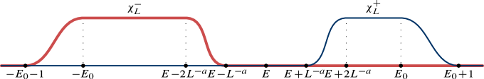
Figure 1. Sketch of the smooth cut-off functions $\chi_{L}^{\pm}$

We are interested in a lower bound for the left-hand side of (3.15) which is proportional to $\ln L$ up to subdominant corrections.

Lemma 4.6.

Let $L>1$. Then

$$\operatorname{tr}\bigl{\{}\bigl{(}1_{(-\infty,E]}(H_{L})1_{(E,\infty)}(H_{L}^{\prime})\bigr{)}^{n}\bigr{\}}$$

$$\geqslant\int_{(0,\infty)^{n}\times(0,\infty)^{n}}\mathrm{d}(u,v)\,(\lvert u\rvert_{1}+\lvert v\rvert_{1})e^{-\lvert u\rvert_{1}-\lvert v\rvert_{1}}\int_{0}^{\infty}\mathrm{d}t\,t^{2n-1}$$

$$\;\;\times\,\operatorname{tr}\bigg{\{}\prod_{j=1}^{n}\sqrt{V}\chi_{L}^{-}(H_{L})e^{(u_{j}+v_{j-1})t(H_{L}-E)}V\chi_{L}^{+}(H_{L}^{\prime})e^{-(u_{j}+v_{j})t(H_{L}^{\prime}-E)}\sqrt{V}\bigg{\}}.$$ (4.21)

• The inequalities

  $$1_{(-\infty,E]}\geqslant\chi_{L}^{-}\quad\text{and}\quad 1_{(E,\infty)}\geqslant\chi_{L}^{+},$$ (4.22)

  together with the cyclicity of the trace, imply

  $$\operatorname{tr}\bigl{\{}\bigl{(}1_{(-\infty,E]}(H_{L})1_{(E,\infty)}(H_{L}^{\prime})\bigr{)}^{n}\bigr{\}}\geqslant\operatorname{tr}\bigl{\{}\bigl{(}\chi_{L}^{-}(H_{L})\chi_{L}^{+}(H_{L}^{\prime})\bigr{)}^{n}\bigr{\}}.$$ (4.23)

  Together with Lemma 4.4, this yields the claim. ∎

Remark 4.7.

In the sequel, we determine the exact asymptotics of the right-hand side of (4.6). Thus it is only the smoothing introduced in Lemma 4.6 which prevents us from determining the exact asymptotics in Theorem 3.4.

The following technical lemma constitutes the core of the arguments in the present subsection.

Lemma 4.8.

For $L>1$, $t\geqslant 0$ and $x\in\mathbb{R}$ we define

$$f_{L}^{t}(x):=\chi_{L}^{-}(x)e^{t(x-E)}\quad\text{and}\quad g_{L}^{t}(x):=\chi_{L}^{+}(x)e^{-t(x-E)},$$ (4.24)

and $h_{L}^{t}$ will stand for either $f_{L}^{t}$ or $g_{L}^{t}$. Let $\varepsilon\in(0,1-a)$ and $M\in\mathbb{N}\setminus\{1\}$. Then there are constants $c>0$, $L_{0}>1$ and a polynomial $Q_{M}$ of degree $M+1$ with non-negative coefficients, such that for every $t\geqslant 0$, every $L\geqslant L_{0}$ and every $\varepsilon\in(0,1-a)$ the estimate

$$\bigl{\lVert}\sqrt{V}\bigl{(}h_{L}^{t}(H_{L}^{(\prime)})-h_{L}^{t}(H^{(\prime)})\bigr{)}\sqrt{V}\bigr{\rVert}\\ \leqslant Q_{M}(t/L^{a})\bigl{(}L^{a-M(1-a-\varepsilon)}+L^{d+a(M+1)}e^{-cL^{\varepsilon}}\bigr{)}$$ (4.25)

holds.

• The proof essentially follows the ideas of a part of the proof in [GKM14, Lemma 3.14]. The idea is to apply the Helffer–Sjöstrand formula to estimate the difference of resolvents, cf. formulae (4.13) and (4.16) in [GKM14]. For a detailed exposition, see [Küt14]. ∎

Before we prove the main assertion of this subsection, we need a spectral-gap estimate.

Lemma 4.9.

There is a constant $C>0$ such that for every $L>1$ and every $t\geqslant 0$ we have

$$\operatorname{tr}\bigl{\{}\sqrt{V}h_{L}^{t}(H^{(\prime)}_{(L)})\sqrt{V}\bigr{\}}\leqslant Ce^{-tL^{-a}},$$ (4.26)

where $h_{L}^{t}\in C_{c}^{\infty}(\mathbb{R})$ is as in Lemma 4.8.

• For the first assertion, note that there is a bounded interval $I\subseteq\mathbb{R}$ such that $h_{L}^{t}\leqslant 1_{I}e^{-tL^{-a}}$ for all $t\geqslant 0$ and $L>1$. Thus,

  $$\operatorname{tr}\bigl{\{}\sqrt{V}h_{L}^{t}(H^{(\prime)}_{(L)})\sqrt{V}\bigr{\}} \leqslant e^{-tL^{-a}}\operatorname{tr}\bigl{\{}\sqrt{V}1_{I}(H^{(\prime)}_{(L)})\sqrt{V}\bigr{\}}$$

  $$\leqslant e^{-tL^{-a}}e^{\sup I}\operatorname{tr}\bigl{\{}\sqrt{V}e^{-H_{(L)}^{(\prime)}}\sqrt{V}\bigr{\}}$$

  $$\leqslant e^{-tL^{-a}}e^{\sup I}\operatorname{tr}\bigl{\{}\sqrt{V}e^{-H^{(\prime)}}\sqrt{V}\bigr{\}}$$ (4.27)

  for $t\geqslant 0$ and $L>1$. The last inequality and the finiteness of $\operatorname{tr}\bigl{\{}\sqrt{V}e^{-H^{(\prime)}}\sqrt{V}\bigr{\}}$ follow from [BHL00, Thm. 6.1]. ∎

The next lemma accomplishes the transition from finite-volume to infinite-volume operators.

Lemma 4.10.

For $L>1$ and $t\geqslant 0$, let $f_{L}^{t},g_{L}^{t}\in C_{c}^{\infty}(\mathbb{R})$ as in Lemma 4.8. Let $u,v\in(0,\infty)^{n}$. Then

$$\int_{0}^{\infty}\mathrm{d}t\;t^{2n-1}\operatorname{tr}\biggl{\lvert}\prod_{j=1}^{n}\sqrt{V}f_{L}^{(u_{j}+v_{j-1})t}(H_{L})Vg_{L}^{(u_{j}+v_{j})t}(H_{L}^{\prime})\sqrt{V}\\ \quad-\prod_{j=1}^{n}\sqrt{V}f_{L}^{(u_{j}+v_{j-1})t}(H)Vg_{L}^{(u_{j}+v_{j})t}(H^{\prime})\sqrt{V}\biggr{\rvert}\\ \quad\leqslant\frac{1}{(\lvert u\rvert_{1}+\lvert v\rvert_{1})^{2n}}\,\mathrm{o}(1)\hfill$$ (4.28)

as $L\to\infty$, where the $\mathrm{o}(1)$-term does not depend on $u$ or $v$. We also used the convention $v_{0}:=v_{n}$.

• To shorten formulas, we introduce a vector $\alpha\in(0,\infty)^{2n}$ via

  $$\alpha_{2j-1}:=u_{j}+v_{j-1}\quad\text{and}\quad\alpha_{2j}:=u_{j}+v_{j}$$ (4.29)

  for $1\leqslant j\leqslant n$ and operators

  $$A^{(L)}_{k}:=\begin{cases}\sqrt{V}f_{L}^{\alpha_{k}t}(H_{(L)})\sqrt{V}&\text{for $k$ odd,}\\ \sqrt{V}g_{L}^{\alpha_{k}t}(H_{(L)}^{\prime})\sqrt{V}&\text{for $k$ even}\end{cases}$$ (4.30)

  for $1\leqslant k\leqslant 2n$. The difference of operator products in (4.28) is then

  $$\prod_{j=1}^{2n}A_{j}^{L}-\prod_{j=1}^{2n}A_{j}=\sum_{k=1}^{2n}A_{1}\dotsm A_{k-1}(A^{L}_{k}-A_{k})A_{k+1}^{L}\dotsm A^{L}_{2n}.$$ (4.31)

  The trace norm of this difference can be estimated using Lemma 4.9: There is a constant $C>0$ such that

  $$\operatorname{tr}\biggl{\lvert}\prod_{j=1}^{2n}A_{j}^{L}-\prod_{j=1}^{2n}A_{j}\biggr{\rvert} \leqslant\sum_{k=1}^{2n}\lVert A_{k}^{L}-A_{k}\rVert\biggl{(}\prod_{j=1}^{k-1}\operatorname{tr}\lvert A_{j}\rvert\biggr{)}\biggl{(}\prod_{j=k+1}^{2n}\operatorname{tr}\lvert A_{j}^{L}\rvert\biggr{)}$$

  $$\leqslant C^{2n-1}\sum_{k=1}^{2n}\lVert A_{k}^{L}-A_{k}\rVert e^{-(\lvert\alpha\rvert_{1}-\alpha_{k})tL^{-a}},$$ (4.32)

  where $\lvert\alpha\rvert_{1}=\alpha_{1}+\dotsb+\alpha_{2n}$ denotes the 1-norm of $\alpha\in(0,\infty)^{2n}$. We estimate the $k$th term in this sum. Let $\varepsilon\in(0,1-a)$ and $M\in\mathbb{N}$. For $L$ sufficiently large, Lemma 4.8 implies

  $$\lVert A_{k}^{L}-A_{k}\rVert e^{-(\lvert\alpha\rvert_{1}-\alpha_{k})tL^{-a}}\\ \leqslant Q_{M}(\alpha_{k}t/L^{a})\bigl{(}L^{a-M(1-a-\varepsilon)}+L^{d+a(M+1)}e^{-cL^{\varepsilon}}\bigr{)}e^{-(\lvert\alpha\rvert_{1}-\alpha_{k})tL^{-a}},$$ (4.33)

  where $Q_{M}(x)=\sum_{\ell=0}^{M+1}q_{\ell}x^{\ell}$ is the polynomial in Lemma 4.8 with non-negative coefficients $q_{\ell}$. Integrating (4.33) yields

  $$\int_{0}^{\infty}\mathrm{d}t\, t^{2n-1}\lVert A_{k}^{L}-A_{k}\rVert e^{-(\lvert\alpha\rvert_{1}-\alpha_{k})tL^{-a}}$$

  $$\leqslant\bigl{(}L^{a-M(1-a-\varepsilon)}+L^{d+a(M+1)}e^{-cL^{\varepsilon}}\bigr{)}$$

  $$\qquad\times\,\sum_{\ell=0}^{M+1}q_{\ell}\int_{0}^{\infty}\!\mathrm{d}t\,t^{2n-1}e^{-(\lvert\alpha\rvert_{1}-\alpha_{k})tL^{-a}}\frac{\alpha_{k}^{\ell}t^{\ell}}{L^{a\ell}}$$

  $$=\bigl{(}L^{a-M(1-a-\varepsilon)}+L^{d+a(M+1)}e^{-cL^{\varepsilon}}\bigr{)}$$

  $$\qquad\times\,\sum_{\ell=0}^{M+1}\frac{q_{\ell}\Gamma(2n+\ell)\alpha_{k}^{\ell}L^{a(2n+\ell)}}{L^{a\ell}(\lvert\alpha\rvert_{1}-\alpha_{k})^{2n+\ell}},$$ (4.34)

  where $\Gamma$ denotes Euler’s Gamma Function. The definition of $\alpha\in(0,\infty)^{2n}$ in (4.29) yields $\lvert\alpha\rvert_{1}=2(\lvert u\rvert_{1}+\lvert v\rvert_{1})$, and thus $\lvert\alpha\rvert_{1}-\alpha_{k}\geqslant\lvert u\rvert_{1}+\lvert v\rvert_{1}\geqslant\alpha_{k}$. This makes the right-hand side of (Proof.) smaller than

  $$C_{M}\frac{L^{2na}}{(\lvert u\rvert_{1}+\lvert v\rvert_{1})^{2n}}\bigl{(}L^{a-M(1-a-\varepsilon)}+L^{d+a(M+1)}e^{-cL^{\varepsilon}}\bigr{)}$$ (4.35)

  with some constant $C_{M}>0$ depending on $Q_{M}$ and $n$. For given $\varepsilon<1-a$, we can choose $M$ large enough for the $L$-terms to vanish as $L\to\infty$. ∎

Using Lemma 4.10, we can rewrite the right-hand side of (4.6).

Corollary 4.11.

The estimate

$$\operatorname{tr} \bigl{\{}\bigl{(}1_{(-\infty,E]}(H_{L})1_{(E,\infty)}(H_{L}^{\prime})\bigr{)}^{n}\bigr{\}}$$

$$\geqslant\int_{(0,\infty)^{n}\times(0,\infty)^{n}}\mathrm{d}(u,v)\,(\lvert u\rvert_{1}+\lvert v\rvert_{1})e^{-\lvert u\rvert_{1}-\lvert v\rvert_{1}}\int_{0}^{\infty}\mathrm{d}t\,t^{2n-1}$$

$$\qquad\times\operatorname{tr}\bigg{\{}\prod_{j=1}^{n}\sqrt{V}\chi_{L}^{-}(H)e^{(u_{j}+v_{j-1})t(H-E)}V\chi_{L}^{+}(H^{\prime})e^{-(u_{j}+v_{j})t(H^{\prime}-E)}\sqrt{V}\bigg{\}}$$

$$\quad+\mathrm{o}(1)$$ (4.36)

holds as $L\to\infty$.

• The claim follows from Lemma 4.6 and Lemma 4.10, which imply that the integral

  $$\int_{(0,\infty)^{n}\times(0,\infty)^{n}}\mathrm{d}(u,v)\,(\lvert u\rvert_{1}+\lvert v\rvert_{1})e^{-\lvert u\rvert_{1}-\lvert v\rvert_{1}}\int_{0}^{\infty}\mathrm{d}t\,t^{2n-1}\\ \quad\times\Biggl{(}\operatorname{tr}\bigg{\{}\prod_{j=1}^{n}\sqrt{V}f_{L}^{(u_{j}+v_{j-1})t}(H_{L})Vg_{L}^{(u_{j}+v_{j})t}(H_{L}^{\prime})\sqrt{V}\bigg{\}}\\ -\operatorname{tr}\bigg{\{}\prod_{j=1}^{n}\sqrt{V}f_{L}^{(u_{j}+v_{j-1})t}(H)Vg_{L}^{(u_{j}+v_{j})t}(H^{\prime})\sqrt{V}\bigg{\}}\Biggr{)}$$ (4.37)

  vanishes in the limit $L\to\infty$, because

  $$\int_{(0,\infty)^{n}\times(0,\infty)^{n}}\mathrm{d}(u,v)\,\frac{e^{-\lvert u\rvert_{1}-\lvert v\rvert_{1}}}{(\lvert u\rvert_{1}+\lvert v\rvert_{1})^{2n-1}}=\frac{1}{(2n-1)!}<\infty,$$ (4.38)

  as can be seen from the coarea formula. ∎

Remark 4.12.

Comparing the smooth cut-off functions $\chi_{L}^{\pm}$ with the ones in [GKM14, Def. 3.13], the difference is that the cut-off functions there have $E$ as the boundary of their support, while the ones here have distance $L^{-a}$ between $E$ and their support. To compensate for this, the $t$-integral has been cut off at $t=L^{-a}$ in [GKM14, Lemma 3.11], which yields a lower bound for $n=1$. For $n\geqslant 2$, it is not immediately clear if the integrand in (4.11) is positive, so cutting off the integration might not result in a lower bound; this is the reason for choosing the cut-off functions different from those in [GKM14].

4.3. Infinite-volume trace expressions

Throughout this subsection, we fix $a\in(0,1)$,  $n\in\mathbb{N}$ and a cut-off energy $E_{0}\geqslant 1$.

In Corollary 4.11, we gave a lower bound on the $n$th term of (3.5) in which only infinite-volume operators occur. In order to control the errors in that step, it was necessary to introduce smoothed versions of indicator functions in (4.22). In the present subsection, our aim is to replace these smoothed functions with discontinuous ones, which will allow us to determine the asymptotics of the resulting expression.

We introduce measures $\mu^{1},\nu^{1}\colon\operatorname{Borel}(\mathbb{R})\to[0,\infty]$ defined by

$$\mu^{1}(A) :=\operatorname{tr}\big{\{}\sqrt{V}1_{A}(H)\sqrt{V}\big{\}}, \nu^{1}(B) :=\operatorname{tr}\big{\{}\sqrt{V}1_{B}(H^{\prime})\sqrt{V}\big{\}}$$ (4.39)

for $A,B\in\operatorname{Borel}(\mathbb{R})$. The expressions in (4.39) are finite for bounded Borel sets as a consequence of [Sim82, Thm. B.9.2].

The absolutely continuous parts of the measures $\mu^{1}$ and $\nu^{1}$ will turn out to be important. To define their densities in an applicable manner, we use a limiting absorption principle due to Birman and Èntina.

Proposition 4.13 ([BÈ67, Lemma 4.3]).

There exists a null set $\mathcal{N}_{0}\subset\mathbb{R}$ such that the limits

$$A(E) :=\lim_{\varepsilon\downarrow 0}\frac{1}{2\varepsilon}\sqrt{V}1_{(E-\varepsilon,E+\varepsilon)}(H)\sqrt{V},$$ (4.40)

$$B(E) :=\lim_{\varepsilon\downarrow 0}\frac{1}{2\varepsilon}\sqrt{V}1_{(E-\varepsilon,E+\varepsilon)}(H^{\prime})\sqrt{V}$$ (4.41)

exist in trace class for all $E\in\mathbb{R}\setminus\mathcal{N}_{0}$ and define non-negative trace class operators $A(E)$ and $B(E)$.

In the next lemma we identify the densities of the absolutely continuous parts of $\mu^{1}$ and $\nu^{1}$. The proof of this lemma follows directly from the definitions.

Lemma 4.14.

The functions $E\mapsto\operatorname{tr}A(E)$, respectively $E\mapsto\operatorname{tr}B(E)$, are locally integrable Lebesgue densities of the absolutely continuous parts of $\mu^{1}$, respectively $\nu^{1}$.

We will need an auxiliary statement for the main result of this subsection.

Lemma 4.15.

Let $\mu$ be a locally finite Borel measure on $\mathbb{R}$. Let $c_{0}>0$ and $0<\varepsilon<\delta<c_{0}$. Then for a.e. $x_{0}\in\mathbb{R}$ there is a constant $C$, depending on $x_{0}$, $c_{0}$ and $\mu$, such that for all $t>0$

$$\int_{[x_{0},x_{0}+\delta]}\mathrm{d}\mu(x)\,e^{-t(x-x_{0})}\leqslant C\frac{1-e^{-t\delta}}{t}$$ (4.42)

and

$$\int_{[x_{0}+\varepsilon,x_{0}+\delta]}\mathrm{d}\mu(x)\,e^{-t(x-x_{0})} \leqslant Ce^{-t\varepsilon/2}\frac{1-e^{-t\delta/2}}{t/2}$$

$$\leqslant C\frac{e^{-t\varepsilon/2}}{t/2}.$$ (4.43)

The exceptional set of values of $x_{0}$ for which the assertion does not hold depends neither on $c_{0}$, $\varepsilon$ nor $\delta$.

• The constant

  $$C:=\sup_{\eta\in(0,c_{0})}\frac{1}{\eta}\mu([x_{0},x_{0}+\eta])$$ (4.44)

  is finite for a.e. $x_{0}\in\mathbb{R}$. We compute using Tonelli’s theorem

  $$\int_{[x_{0},x_{0}+\delta]} \mathrm{d}\mu(x)\,e^{-t(x-x_{0})}$$

  $$=\int_{[x_{0},x_{0}+\delta]}\mathrm{d}\mu(x)\Bigl{(}e^{-t\delta}+t\int_{x}^{x_{0}+\delta}\mathrm{d}\xi\,e^{-t(\xi-x_{0})}\Bigr{)}$$

  $$=\delta e^{-t\delta}\frac{1}{\delta}\mu([x_{0},x_{0}+\delta])+t\int_{x_{0}}^{x_{0}+\delta}\mathrm{d}\xi\int_{[x_{0},\xi]}\mathrm{d}\mu(x)\,e^{-t(\xi-x_{0})}$$

  $$\leqslant C\delta e^{-t\delta}+t\int_{x_{0}}^{x_{0}+\delta}\mathrm{d}\xi\,e^{-t(\xi-x_{0})}\frac{\xi-x_{0}}{\xi-x_{0}}\mu([x_{0},\xi])$$

  $$\leqslant C\delta e^{-t\delta}+Ct\int_{0}^{\delta}\mathrm{d}\xi\,\xi e^{-t\xi}$$

  $$=C\frac{1-e^{-t\delta}}{t}.$$ (4.45)

  The second assertion follows from the first one and the bound $e^{-t(x-x_{0})}\leqslant e^{-t\varepsilon/2}e^{-t(x-x_{0})/2}$ for $\varepsilon\leqslant x-x_{0}\leqslant\delta$. ∎

Definition 4.16.

• For $k\in\mathbb{N}$, we define

  $${}{}I_{k}:=\int_{(0,\infty)^{k}}\mathrm{d}u\,\frac{\lvert u\rvert_{1}e^{-\lvert u\rvert_{1}}}{\prod_{j=1}^{k}(u_{j}+u_{j+1})},$$ (4.46)

  where $u_{k+1}:=u_{1}$ for $u\in\mathbb{R}^{k}$.

• We define discontinuous $L$-independent functions $\chi^{\pm}\colon\mathbb{R}\to[0,1]$ by

  $$\chi^{-}:=\max\{\chi^{-}_{L},1_{[-E_{0},E)}\}\quad\text{and}\quad\chi^{+}:=\max\{\chi^{+}_{L},1_{(E,E_{0}]}\}.$$ (4.47)

Remarks 4.17.

• The integral $I_{k}$ will be discussed further in Subsection 4.5; in particular, $I_{k}$ is finite for every $k\in\mathbb{N}$.

• The functions $\chi_{L}^{\pm}$ converge pointwise to $\chi^{\pm}$ as $L\to\infty$. They are obtained from replacing the smooth $L$-dependent part by a discontinuous step at $E$. Fig. 2 illustrates the behaviour of $\chi^{\pm}$.

Figure 2. Sketch of the discontinuous cut-off functions $\chi^{\pm}$

The following lemma is the main result of the current section.

Lemma 4.18.

There is a null set $\mathcal{N}\subseteq\mathbb{R}$ which does not depend on $a$, $n$ and $E_{0}$, such that for every $E\in[-E_{0},E_{0}]\setminus\mathcal{N}$,

$$\int_{0}^{\infty}\mathrm{d}t\,t^{2n-1} \int_{(0,\infty)^{n}\times(0,\infty)^{n}}\mathrm{d}(u,v)\,(\lvert u\rvert_{1}+\lvert v\rvert_{1})e^{-\lvert u\rvert_{1}-\lvert v\rvert_{1}}$$

$$\quad\;\times\!\Biggl{[}\operatorname{tr}\bigg{\{}\prod_{j=1}^{n}\!\sqrt{V}\chi^{-}_{L}(H)e^{(u_{j}+v_{j-1})t(H-E)}\sqrt{V}$$

$$\hskip 93.89418pt\times\;\sqrt{V}\chi^{+}_{L}(H^{\prime})e^{-(u_{j}+v_{j})t(H^{\prime}-E)}\sqrt{V}\bigg{\}}$$

$$\qquad\quad-e^{-tL^{-a}}\operatorname{tr}\bigg{\{}\prod_{j=1}^{n}\!\sqrt{V}\chi^{-}(H)e^{(u_{j}+v_{j-1})t(H-E)}\sqrt{V}$$

$$\hskip 93.89418pt\times\;\sqrt{V}\chi^{+}(H^{\prime})e^{-(u_{j}+v_{j})t(H^{\prime}-E)}\sqrt{V}\bigg{\}}\Biggr{]}$$

$$\quad=\mathrm{O}(1)$$ (4.48)

as $L\to\infty$, where the $\mathrm{O}(1)$-term depends on $a$, $n$, $E$ and $E_{0}$.

• First, notice that if $f_{j},g_{j}$ are bounded measurable functions of compact support for $1\leqslant j\leqslant n$, then

  $$\operatorname{tr}\prod_{j=1}^{n}\biggl{\lvert}\sqrt{V}f_{j}(H)Vg_{j}(H^{\prime})\sqrt{V}\biggr{\rvert} \leqslant\prod_{j=1}^{n}\operatorname{tr}\Bigl{\{}\sqrt{V}f_{j}(H)\sqrt{V}\Bigr{\}}\operatorname{tr}\Bigl{\{}\sqrt{V}g_{j}(H^{\prime})\sqrt{V}\Bigr{\}}$$

  $$=\int_{\mathbb{R}^{n}}\mathrm{d}\mu^{n}(x)\int_{\mathbb{R}^{n}}\mathrm{d}\nu^{n}(y)\prod_{j=1}^{n}f_{j}(x_{j})g_{j}(y_{j}),$$ (4.49)

  where we wrote $\mu^{n}$ and $\nu^{n}$ for the $n$-fold product measure of $\mu^{1}$ and $\nu^{1}$, respectively.

  For brevity, let $\delta:=L^{-a}$. We introduce a vector $\alpha\in(0,\infty)^{2n}$ via

  $$\alpha_{2j-1}:=u_{j}+v_{j-1}\quad\text{and}\quad\alpha_{2j}:=u_{j}+v_{j}$$ (4.50)

  for $1\leqslant j\leqslant n$ and operators

  $$A^{(L)}_{k}:=\begin{cases}\sqrt{V}\chi^{-}_{(L)}(H)e^{\alpha_{k}t(H-E)}\sqrt{V}&\text{for $k$ odd,}\\ \sqrt{V}\chi^{+}_{(L)}(H^{\prime})e^{-\alpha_{k}t(H^{\prime}-E)}\sqrt{V}&\text{for $k$ even}\end{cases}$$ (4.51)

  for $1\leqslant k\leqslant 2n$. The difference of operator products in (4.18) then equals

  $$\prod_{j=1}^{2n}A_{j}^{L}-e^{-t\delta}\prod_{j=1}^{2n}A_{j}=e^{-t\delta}\Bigl{(}\prod_{j=1}^{2n}A_{j}^{L}-\prod_{j=1}^{2n}A_{j}\Bigr{)}+(1-e^{-t\delta})\prod_{j=1}^{2n}A_{j}^{L},$$ (4.52)

  where as in (4.31),

  $$\prod_{j=1}^{2n}A_{j}^{L}-\prod_{j=1}^{2n}A_{j}=\sum_{k=1}^{2n}A_{1}\dotsm A_{k-1}(A^{L}_{k}-A_{k})A_{k+1}^{L}\dotsm A^{L}_{2n}.$$ (4.53)

  We will treat the two terms on the right-hand side of (4.52) individually. For the first term, we estimate the $k$th term in (4.53). We will carry out the argument in the case where $k$ is even. The argument is similar for odd $k$. Since $0\leqslant\chi^{+}-\chi^{+}_{L}\leqslant 1_{[E,E+2\delta]}$,  $\chi_{(L)}^{-}\leqslant 1_{[-E_{0}-1,E]}$ and $\chi_{(L)}^{+}\leqslant 1_{[E,E_{0}+1]}$, (Proof.) implies

  $$\operatorname{tr}\Bigl{\lvert}A_{1}\dotsm A_{k-1}(A^{L}_{k}-A_{k})A_{k+1}^{L}\dotsm A^{L}_{2n}\Bigr{\rvert}$$

  $$\quad\leqslant\int_{[-E_{0}-1,E]^{n}}\mathrm{d}\mu^{n}(x)\int_{[E,E_{0}+1]^{n}}\mathrm{d}\nu^{n}(y)\,1_{[E,E+2\delta]}(y_{k})$$

  $$\qquad\qquad\times\exp\Bigl{(}-t\sum_{j=1}^{n}\bigl{(}(u_{j}+v_{j})(y_{j}-E)-(u_{j}+v_{j-1})(x_{j}-E)\bigr{)}\Bigr{)}$$

  $$\quad\leqslant C\frac{1-e^{-2(u_{k}+v_{k})t\delta}}{t}\frac{1}{t^{2n-1}}\frac{1}{\prod_{j=1}^{n}(u_{j}+v_{j})(u_{j}+v_{j-1})},$$ (4.54)

  where $C$ is some finite constant and the last inequality follows for a.e. $E\in[-E_{0},E_{0}]$ from applying Lemma 4.15 to every integral and the estimate $1-e^{-tx}\leqslant 1$ to all but the $k$th term. Using the bound $1-e^{-2(u_{k}+v_{k})t\delta}\leqslant 2(u_{k}+v_{k})t\delta$, we conclude

  $$e^{-t\delta}\operatorname{tr}\biggl{\lvert}\prod_{j=1}^{2n}A_{j}^{L}-\prod_{j=1}^{2n}A_{j}\biggr{\rvert}\leqslant 4C\frac{\delta e^{-t\delta}}{t^{2n-1}}\frac{\lvert u\rvert_{1}+\lvert v\rvert_{1}}{\prod_{j=1}^{n}(u_{j}+v_{j})(u_{j}+v_{j-1})},$$ (4.55)

  and therefore

  $$\int_{0}^{\infty} \mathrm{d}t\,t^{2n-1}\int_{(0,\infty)^{n}\times(0,\infty)^{n}}\mathrm{d}(u,v)\,(\lvert u\rvert_{1}+\lvert v\rvert_{1})e^{-\lvert u\rvert_{1}-\lvert v\rvert_{1}}$$

  $$\qquad\times e^{-t\delta}\operatorname{tr}\biggl{\lvert}\prod_{j=1}^{2n}A_{j}^{L}-\prod_{j=1}^{2n}A_{j}\biggr{\rvert}$$

  $$\;\leqslant 4C\int_{0}^{\infty}\mathrm{d}t\,\delta e^{-t\delta}\int_{(0,\infty)^{n}\times(0,\infty)^{n}}\mathrm{d}(u,v)\,\frac{(\lvert u\rvert_{1}+\lvert v\rvert_{1})^{2}e^{-\lvert u\rvert_{1}-\lvert v\rvert_{1}}}{\prod_{j=1}^{n}(u_{j}+v_{j})(u_{j}+v_{j-1})}.$$ (4.56)

  Here, the $t$-integral yields $1$ for every $\delta>0$, and the $(u,v)$-integral is finite since

  $$\int_{(0,\infty)^{n}\times(0,\infty)^{n}}\mathrm{d}(u,v)\,\frac{(\lvert u\rvert_{1}+\lvert v\rvert_{1})^{2}e^{-\lvert u\rvert_{1}-\lvert v\rvert_{1}}}{\prod_{j=1}^{n}(u_{j}+v_{j})(u_{j}+v_{j-1})}\\ \qquad\qquad\leqslant\int_{(0,\infty)^{n}\times(0,\infty)^{n}}\mathrm{d}(u,v)\,\frac{(\lvert u\rvert_{1}+\lvert v\rvert_{1})e^{-\lvert u\rvert_{1}/2-\lvert v\rvert_{1}/2}}{\prod_{j=1}^{n}(u_{j}+v_{j})(u_{j}+v_{j-1})}\hfill\\ \qquad\qquad=2I_{2n}<\infty,\hfill$$ (4.57)

  with $I_{2n}$ as in Definition 4.16. This shows that the integral of the trace norm of the first term on the right-hand side of (4.52) yields an error that remains finite as $L\to\infty$.

  The trace norm of the second term on the right-hand side of (4.52) is

  $$(1-e^{-t\delta})\operatorname{tr}\biggl{\lvert}\prod_{j=1}^{2n}A_{j}^{L}\biggr{\rvert}$$

  $$\leqslant(1-e^{-t\delta})\int_{[-E_{0}-1,E-\delta]^{n}}\mathrm{d}\mu^{n}(x)\int_{[E+\delta,E_{0}+1]^{n}}\mathrm{d}\nu^{n}(y)\,$$

  $$\qquad\times\exp\Bigl{(}-t\sum_{j=1}^{n}\bigl{(}(u_{j}+v_{j})(y_{j}-E)-(u_{j}+v_{j-1})(x_{j}-E)\bigr{)}\Bigr{)}$$

  $$\leqslant C(1-e^{-t\delta})\prod_{j=1}^{n}\frac{e^{-(u_{j}+v_{j-1})t\delta/2}e^{-(u_{j}+v_{j})t\delta/2}}{(u_{j}+v_{j-1})(u_{j}+v_{j})(t/2)^{2}}$$

  $$=2^{2n}C\frac{(1-e^{-t\delta})e^{-(\lvert u\rvert_{1}+\lvert v\rvert_{1})t\delta}t^{-2n}}{\prod_{j=1}^{n}(u_{j}+v_{j})(u_{j}+v_{j-1})},$$ (4.58)

  where the first inequality is a consequence of $\chi_{(L)}^{-}\leqslant 1_{[-E_{0}-1,E]}$ and $\chi_{(L)}^{+}\leqslant 1_{[E,E_{0}+1]}$, and the second inequality follows for a.e. $E\in[-E_{0},E_{0}]$ from Lemma 4.15. Now, we perform the $t$- and $(u,v)$-integration

  $$\int_{(0,\infty)^{n}\times(0,\infty)^{n}}\mathrm{d}(u,v)\,(\lvert u\rvert_{1}+\lvert v\rvert_{1})e^{-\lvert u\rvert_{1}-\lvert v\rvert_{1}}\int_{0}^{\infty}\mathrm{d}t\,t^{2n-1}$$

  $$\hskip 80.00012pt\times\frac{(1-e^{-t\delta})e^{-(\lvert u\rvert_{1}+\lvert v\rvert_{1})t\delta}t^{-2n}}{\prod_{j=1}^{n}(u_{j}+v_{j})(u_{j}+v_{j-1})},$$

  $$=\int_{(0,\infty)^{n}\times(0,\infty)^{n}}\mathrm{d}(u,v)\int_{0}^{\infty}\mathrm{d}t\,\frac{(1-e^{-t})e^{-(1+t)(\lvert u\rvert_{1}+\lvert v\rvert_{1})}(\lvert u\rvert_{1}+\lvert v\rvert_{1})}{t\,\prod_{j=1}^{n}(u_{j}+v_{j})(u_{j}+v_{j-1})}$$

  $$=I_{2n}\int_{0}^{\infty}\mathrm{d}t\,\frac{1-e^{-t}}{t^{2}+t}<\infty,$$ (4.59)

  where we performed the successive changes of variables $t\delta\rightsquigarrow t$ and $(1+t)(u,v)\rightsquigarrow(u,v)$. ∎

Corollary 4.19.

For a.e. $E\in[-E_{0},E_{0}]$, we have

$$\operatorname{tr}\bigl{\{}\bigl{(}1_{(-\infty,E]}(H_{L})1_{(E,\infty)}(H_{L}^{\prime})\bigr{)}^{n}\bigr{\}}$$

$$\geqslant\int_{(0,\infty)^{n}\times(0,\infty)^{n}}\mathrm{d}(u,v)\,(\lvert u\rvert_{1}+\lvert v\rvert_{1})e^{-\lvert u\rvert_{1}-\lvert v\rvert_{1}}\int_{0}^{\infty}\mathrm{d}t\,t^{2n-1}e^{-tL^{-a}}$$

$$\qquad\times\operatorname{tr}\bigg{\{}\prod_{j=1}^{n}\sqrt{V}\chi^{-}(H)e^{(u_{j}+v_{j-1})t(H-E)}V\chi^{+}(H^{\prime})e^{-(u_{j}+v_{j})t(H^{\prime}-E)}\sqrt{V}\bigg{\}}$$

$$\quad+\mathrm{O}(1)$$ (4.60)

as $L\to\infty$. The null set of exceptional energies does not depend on $a$, $n$ and $E_{0}$.

• We combine Corollary 4.11 and Lemma 4.18. ∎

4.4. The logarithmic divergence

Throughout this subsection, we fix $a\in(0,1)$, $n\in\mathbb{N}$ and $E_{0}\geqslant 1$.

The goal is to determine the asymptotics of the right-hand side of (4.19).

Lemma 4.20.

For a.e. $E\in[-E_{0},E_{0}]$,

$$A_{t}(E) :=\sqrt{V}te^{t(H-E)}\chi^{-}(H)\sqrt{V}\to A(E),$$ (4.61)

$$B_{t}(E) :=\sqrt{V}te^{-t(H^{\prime}-E)}\chi^{+}(H^{\prime})\sqrt{V}\to B(E)$$

as $t\to\infty$, where the convergences are in trace class. Moreover,

$$\sup_{t\geqslant 0}\lVert A_{t}(E)\rVert \leqslant\sup_{t\geqslant 0}\operatorname{tr}A_{t}(E)<\infty,$$ (4.62)

$$\sup_{t\geqslant 0}\lVert B_{t}(E)\rVert \leqslant\sup_{t\geqslant 0}\operatorname{tr}B_{t}(E)<\infty.$$

• We follow [GKM14, Lemma 3.16] and treat the operator $B_{t}(E)$; the assertions for $A_{t}(E)$ can be proved using analogous arguments. Recall that $B_{t}(E)$ is non-negative. For (4.61), we show (1) convergence of the trace norms and (2) weak convergence of the operators. Together, this implies convergence in trace class via [Sim05, Addendum H].

  For the trace norms, we compute

  $$\operatorname{tr}B_{t}(E) =\operatorname{tr}\bigl{\{}\sqrt{V}te^{-t(H^{\prime}-E)}\chi^{+}(H^{\prime})\sqrt{V}\bigr{\}}$$

  $$=\int_{[E,E_{0}]}\mathrm{d}\nu^{1}(y)\,te^{-t(y-E)}+\int_{[E_{0},E_{0}+1]}\mathrm{d}\nu^{1}(y)\,\chi^{+}(y)te^{-t(y-E)}$$ (4.63)

  where the second term converges to zero as $t\to\infty$ for $E<E_{0}$. The first term can be written as

  $$\int_{[E,E_{0}]}\mathrm{d}\nu^{1}(y)\,te^{-t(y-E)}=(\nu^{1}_{E_{0}}*\varrho_{t})(E),$$ (4.64)

  where we introduced the restricted (finite) measure $\nu_{E_{0}}^{1}(M):=\nu^{1}(M\cap[-E_{0},E_{0}])$ for $M\in\operatorname{Borel}(\mathbb{R})$ and the approximation of the identity $x\mapsto\varrho_{t}(x):=te^{tx}1_{(-\infty,0)}(x)$. As $t\to\infty$, the convolution in (4.64) converges for a.e. $E\in[-E_{0},E_{0}]$ to $\frac{\mathrm{d}\nu_{\mathrm{ac}}^{1}}{\mathrm{d}E}=\operatorname{tr}B(E)$, see e.g. [MS13, Subsec. 2.4.1]. Thus, the trace norm of $B_{t}(E)$ converges to that of $B(E)$ as $t\to\infty$. This, together with the continuity of $[0,\infty)\ni t\mapsto\operatorname{tr}B_{t}(E)$, which can be seen from (Proof.), implies (4.62).

  For the weak convergence, take some dense countable set $\mathcal{D}\subseteq L^{2}(\mathbb{R}^{d})$. Then by a similar delta-argument as above,

  $$\lim_{t\to\infty}\langle\varphi,B_{t}(E)\psi\rangle=\langle\varphi,B(E)\psi\rangle$$ (4.65)

  for all $\varphi,\psi\in\mathcal{D}$ and all $E\in[-E_{0},E_{0}]$ outside a null set depending on $\mathcal{D}$. Together with (4.62), this proves weak convergence to $B(E)$ for a.e. $E\in[-E_{0},E_{0}]$, see [Wei80, Thm. 4.26]. ∎

The following quantity will enter the asymptotics we set out to prove.

Definition 4.21.

For $E\in\mathbb{R}\setminus\mathcal{N}_{0}$, let

$$\eta_{2n}(E):=\operatorname{tr}\bigl{\{}\bigl{(}A(E)B(E)\bigr{)}^{n}\bigr{\}}$$ (4.66)

and extend it trivially to a function $\eta_{2n}\colon\mathbb{R}\to[0,\infty)$. The non-negativity of (4.66) can be seen from the cyclicity of the trace.

The next corollary will show that the trace expression on the right-hand side of (4.19), times an appropriate power of $t$, converges to $\eta_{2n}(E)$ in the $t\to\infty$ limit.

Corollary 4.22.

Let $\alpha_{1},\dotsc,\alpha_{n},\beta_{1},\dotsc,\beta_{n}>0$. Then for a.e. $E\in[-E_{0},E_{0}]$

$$t^{2n}\operatorname{tr}\bigg{\{}\prod_{j=1}^{n}\sqrt{V}\chi^{-}(H)\alpha_{j}e^{\alpha_{j}t(H-E)}V\chi^{+}(H^{\prime})\beta_{j}e^{-\beta_{j}t(H^{\prime}-E)}\sqrt{V}\bigg{\}}\to\eta_{2n}(E)$$ (4.67)

as $t\to\infty$.

• Using the notation of Lemma 4.20, we have to show

  $$\biggl{\lvert}\operatorname{tr}\bigg{\{}\prod_{j=1}^{n}A_{\alpha_{j}t}(E)B_{\beta_{j}t}(E)\bigg{\}}-\operatorname{tr}\bigl{\{}\bigl{(}A(E)B(E)\bigr{)}^{n}\bigr{\}}\biggr{\rvert}\to 0$$ (4.68)

  as $t\to\infty$. By Lemma 4.20, $\operatorname{tr}\lvert A_{\alpha_{j}t}(E)-A(E)\rvert\to 0$ and $\operatorname{tr}\lvert B_{\beta_{j}t}(E)-B(E)\rvert\to 0$ as $t\to\infty$, while $\sup_{t\geqslant 0}\lVert A_{t}(E)\rVert$ and $\sup_{t\geqslant 0}\lVert B_{t}(E)\rVert$ are finite. Writing the difference of operator products in (4.68) as in (4.31), this proves the corollary. ∎

Lemma 4.23.

Let $f\in L^{1}_{\mathrm{loc}}(\mathbb{R})$ and suppose $\lim_{t\to\infty}f(t)$ exists. Then

$$\lim_{t\to\infty}f(t)=-\lim_{s\downarrow 0}\frac{1}{\ln s}\int_{1}^{\infty}\mathrm{d}t\,t^{-1}e^{-st}f(t).$$ (4.69)

• Take a compact interval $[s_{0},c]\subseteq(0,\infty)$. Then

  $$\frac{\mathrm{d}}{\mathrm{d}{s}}\int_{1}^{\infty}\mathrm{d}t\,t^{-1}e^{-st}f(t)=-\int_{1}^{\infty}\mathrm{d}t\,e^{-st}f(t)$$ (4.70)

  for $s\in[s_{0},c]$, because $\bigl{\lvert}\frac{\mathrm{d}}{\mathrm{d}{s}}t^{-1}e^{-st}f(t)\bigr{\rvert}\leqslant e^{-s_{0}t}\lvert f(t)\rvert$, which is integrable on $[1,\infty)$. Therefore (4.70) holds for all $s>0$. If $\lim_{s\downarrow 0}\int_{1}^{\infty}\mathrm{d}t\,t^{-1}e^{-st}f(t)$ exists, then $\lim_{t\to\infty}f(t)=0$ and the assertion holds. Otherwise,

  $$-\lim_{s\downarrow 0}\frac{1}{\ln s}\int_{1}^{\infty}\mathrm{d}t\,t^{-1}e^{-st}f(t) =\lim_{s\downarrow 0}\frac{1}{1/s}\int_{1}^{\infty}\mathrm{d}t\,e^{-st}f(t)$$

  $$=\lim_{s\downarrow 0}s\int_{0}^{\infty}\mathrm{d}t\,e^{-st}f(t)$$

  $$=\lim_{t\to\infty}f(t),$$ (4.71)

  where the last equality is the statement of the classical final-value theorem, see [Doe74, Thm. 34.3]. ∎

We are now ready to compute the asymptotics of the right-hand side of (4.19)

Theorem 4.24.

For a.e. $E\in[-E_{0},E_{0}]$,

$$\lim_{L\to\infty}\frac{1}{a\ln L}\int_{0}^{\infty}\mathrm{d}t\,t^{2n-1}e^{-tL^{-a}}\!\int_{(0,\infty)^{n}\times(0,\infty)^{n}}\!\mathrm{d}(u,v)\,(\lvert u\rvert_{1}+\lvert v\rvert_{1})e^{-\lvert u\rvert_{1}-\lvert v\rvert_{1}}$$

$$\quad\times\operatorname{tr}\bigg{\{}\prod_{j=1}^{n}\sqrt{V}\chi^{-}(H)e^{(u_{j}+v_{j-1})t(H-E)}V\chi^{+}(H^{\prime})e^{-(u_{j}+v_{j})t(H^{\prime}-E)}\sqrt{V}\bigg{\}}$$

$$=I_{2n}\eta_{2n}(E).$$ (4.72)

• Let $u,v\in(0,\infty)^{n}$ and define

  $$Z(u,v):=\prod_{j=1}^{n}(u_{j}+v_{j-1})(u_{j}+v_{j}).$$ (4.73)

  Using the notation of Lemma 4.20, we see that

  $$Z(u,v) t^{2n}\operatorname{tr}\bigg{\{}\prod_{j=1}^{n}\sqrt{V}\chi^{-}(H)e^{(u_{j}+v_{j-1})t(H-E)}\sqrt{V}$$

  $$\hskip 42.67912pt\times\sqrt{V}\chi^{+}(H^{\prime})e^{-(u_{j}+v_{j})t(H^{\prime}-E)}\sqrt{V}\bigg{\}}$$

  $$=\operatorname{tr}\bigg{\{}\prod_{j=1}^{n}A_{(u_{j}+v_{j-1})t}(E)B_{(u_{j}+v_{j})t}(E)\bigg{\}},$$ (4.74)

  where

  $$\biggl{\lvert}\operatorname{tr}\bigg{\{}\prod_{j=1}^{n}A_{(u_{j}+v_{j-1})t}(E)B_{(u_{j}+v_{j})t}(E)\bigg{\}}\biggr{\rvert}\leqslant\bigl{(}\sup_{t\geqslant 0}\operatorname{tr}A_{t}(E)\sup_{t\geqslant 0}\operatorname{tr}B_{t}(E)\bigr{)}^{n}<\infty.$$ (4.75)

  By Corollary 4.22,

  $$\lim_{t\to\infty}\operatorname{tr}\bigg{\{}\prod_{j=1}^{n}A_{(u_{j}+v_{j-1})t}(E)B_{(u_{j}+v_{j})t}(E)\bigg{\}}=\eta_{2n}(E)$$ (4.76)

  for all $u,v\in(0,\infty)^{n}$. By Remark 4.17 (i),

  $$I_{2n}=\int_{(0,\infty)^{n}\times(0,\infty)^{n}}\mathrm{d}(u,v)\,\frac{(\lvert u\rvert_{1}+\lvert v\rvert_{1})e^{-\lvert u\rvert_{1}-\lvert v\rvert_{1}}}{Z(u,v)}<\infty.$$ (4.77)

  Equations (4.75) to (4.77) supply the assumptions of the dominated convergence theorem. It yields the convergence

  $$\lim_{t\to\infty}f(t)=I_{2n}\eta_{2n}(E)$$ (4.78)

  for

  $$f(t):={} \int_{(0,\infty)^{n}\times(0,\infty)^{n}}\mathrm{d}(u,v)\,(\lvert u\rvert_{1}+\lvert v\rvert_{1})e^{-\lvert u\rvert_{1}-\lvert v\rvert_{1}}\;t^{2n}$$

  $$\times\operatorname{tr}\bigg{\{}\prod_{j=1}^{n}\sqrt{V}\chi^{-}(H)e^{(u_{j}+v_{j-1})t(H-E)}\sqrt{V}$$

  $$\hskip 45.52458pt\times\sqrt{V}\chi^{+}(H^{\prime})e^{-(u_{j}+v_{j})t(H^{\prime}-E)}\sqrt{V}\bigg{\}}$$

  $$={} \int_{(0,\infty)^{n}\times(0,\infty)^{n}}\mathrm{d}(u,v)\,\frac{(\lvert u\rvert_{1}+\lvert v\rvert_{1})e^{-\lvert u\rvert_{1}-\lvert v\rvert_{1}}}{Z(u,v)}$$

  $$\times\operatorname{tr}\bigg{\{}\prod_{j=1}^{n}A_{(u_{j}+v_{j-1})t}(E)B_{(u_{j}+v_{j})t}(E)\bigg{\}},$$ (4.79)

  where $t>0$. The assertion (4.24) follows from

  $$-\lim_{L\to\infty}\frac{1}{\ln(L^{-a})}\int_{0}^{\infty}\mathrm{d}t\,t^{-1}e^{-tL^{-a}}f(t)=\lim_{t\to\infty}f(t),$$ (4.80)

  which is a consequence of Lemma 4.23 and of

  $$\sup_{L>1}\int_{0}^{1}\mathrm{d}t\,t^{-1}e^{-tL^{-a}}f(t)<\infty.$$ (4.81)

  ∎

Corollary 4.25.

For a.e. $E\in\mathbb{R}$, the estimate

$$\operatorname{tr}\bigl{\{}\bigl{(}1_{(-\infty,E]}(H_{L})1_{(E,\infty)}(H_{L}^{\prime})\bigr{)}^{n}\bigr{\}}\geqslant\ln L\;I_{2n}\eta_{2n}(E)+\mathrm{o}(\ln L)$$ (4.82)

holds, where the $\mathrm{o}(\ln L)$-term depends on $n$ and $E$.

• We deduce from Theorem 4.24, Corollary 4.19 and from the arbitrariness of $E_{0}$ that

  $$\liminf_{L\to\infty}\frac{\operatorname{tr}\bigl{\{}\bigl{(}1_{(-\infty,E]}(H_{L})1_{(E,\infty)}(H_{L}^{\prime})\bigr{)}^{n}\bigr{\}}}{\ln L}\geqslant a\,I_{2n}\eta_{2n}(E)$$ (4.83)

  for arbitrary $a\in(0,1)$ and a.e. $E\in\mathbb{R}$. Thus (4.83) holds for $a=1$ and a.e. $E\in\mathbb{R}$. By definition of the limit inferior, this implies the claim. ∎

4.5. A multi-dimensional integral related to the Hilbert matrix

In this subsection, we compute the coefficient of $\eta_{2n}(E)$ in the asymptotics in Corollary 4.25, i.e., we compute the integral

$$I_{n}=\int_{(0,\infty)^{n}}\mathrm{d}u\,\frac{\lvert u\rvert_{1}e^{-\lvert u\rvert_{1}}}{\prod_{j=1}^{n}(u_{j}+u_{j+1})}$$ (4.84)

in Definition 4.16 (i). Here, we use the convention $u_{n+1}=u_{1}$ for $u\in\mathbb{R}^{n}$. We prove

Theorem 4.26.

Let $n\in\mathbb{N}_{\geqslant 2}$. Then

$$I_{n}=(2\pi)^{n-2}\frac{\bigl{(}\Gamma(\frac{n}{2})\bigr{)}^{2}}{\Gamma(n)}.$$ (4.85)

This implies

$$I_{2n}=(2\pi)^{2n-2}\frac{[(n-1)!]^{2}}{(2n-1)!}=nJ_{2n}$$ (4.86)

for $n\in\mathbb{N}$, where $J_{2n}$ was defined in (3.16).

We begin with an elementary lemma.

Lemma 4.27.

Let $n\in\mathbb{N}_{\geqslant 2}$. Then

$$I_{n}=\frac{n}{2}\int_{(0,\infty)^{n}}\mathrm{d}u\,\frac{e^{-\lvert u\rvert_{1}}}{\prod_{j=1}^{n-1}(u_{j}+u_{j+1})}.$$ (4.87)

• Using the symmetry of $I_{n}$ in the components of $u$, we compute

  $$I_{n} =\frac{1}{2}\int_{(0,\infty)^{n}}\mathrm{d}u\,e^{-\lvert u\rvert_{1}}\frac{2\lvert u\rvert_{1}}{\prod_{j=1}^{n}(u_{j}+u_{j+1})}$$

  $$=\frac{1}{2}\sum_{k=1}^{n}\int_{(0,\infty)^{n}}\mathrm{d}u\,e^{-\lvert u\rvert_{1}}\frac{u_{k}+u_{k+1}}{\prod_{j=1}^{n}(u_{j}+u_{j+1})}$$

  $$=\frac{n}{2}\int_{(0,\infty)^{n}}\mathrm{d}u\,\frac{e^{-\lvert u\rvert_{1}}}{\prod_{j=1}^{n-1}(u_{j}+u_{j+1})}.$$ (4.88)

  ∎

In the sequel, we will work with the Rosenblum–Rovnyak integral operator $T\colon L^{2}((0,\infty))\to L^{2}((0,\infty))$, see [Ros58] and [Rov70], defined by

$$(Tf)(x):=\int_{0}^{\infty}\mathrm{d}y\,\frac{e^{-(x+y)/2}}{x+y}f(y)$$ (4.89)

for $f\in L^{2}((0,\infty))$ and $x\in(0,\infty)$. This operator can be explicitly diagonalised. Following [Yaf10, Sec. 4.2], we define the Kontorovich–Lebedev transform, i.e. the unitary operator $U\colon L^{2}((0,\infty))\to L^{2}((0,\infty))$,

$$(Uf)(k):=\pi^{-1}\sqrt{k\sinh(2\pi k)}\,\lvert\Gamma(1/2-ik)\rvert\int_{0}^{\infty}\mathrm{d}x\,x^{-1}W_{0,ik}(x)f(x)$$ (4.90)

for $f\in L^{2}((0,\infty))$ and $k\in(0,\infty)$, where $W_{0,ik}$ denotes the Whittaker function, see [DLMF, Sec. 13.14] or [GR07, Sec. 9.22–9.23]. Then, the spectral representation due to Rosenblum reads

$$(UTf)(k)=\frac{\pi}{\cosh(k\pi)}(Uf)(k)$$ (4.91)

for $f\in L^{2}((0,\infty))$ and $k\in(0,\infty)$, see [Yaf10, Prop. 4.1].

• Let $n\in\mathbb{N}_{\geqslant 2}$. From (4.87) and (4.89), we see that

  $$\frac{2}{n}I_{n}=\bigl{\langle}\phi_{0},T^{n-1}\phi_{0}\bigr{\rangle}_{L^{2}((0,\infty))}$$ (4.92)

  with $\phi_{0}(x):=e^{-x/2}$. From (4.91) and (4.92), we obtain

  $$\frac{2}{n}I_{n}=\bigl{\langle}U\phi_{0},UT^{n-1}\phi_{0}\bigr{\rangle}_{L^{2}((0,\infty))}=\int_{0}^{\infty}\mathrm{d}k\,\lvert(U\phi_{0})(k)\rvert^{2}\Bigl{(}\frac{\pi}{\cosh(k\pi)}\Bigr{)}^{n-1}.$$ (4.93)

  In order to compute $U\phi_{0}$, we employ the classical formula

  $$\lvert\Gamma(1/2-ik)\rvert^{2}=\frac{\pi}{\cosh(k\pi)}$$ (4.94)

  for $k\in\mathbb{R}$, which is a consequence of the reflection formula for the Gamma function, and

  $$\int_{0}^{\infty}\mathrm{d}x\,x^{-1}W_{0,ik}(x)e^{-x/2}=\frac{\pi}{\cosh(k\pi)}\mathchoice{\qquad(k>0)}{\,\ (k>0)}{\,(k>0)}{\,(k>0)},$$ (4.95)

  which follows from the special case $z=1/2$ and $\nu=\kappa=0$ in [DLMF, Eq. 13.23.4]. From (4.90), (4.94), and (4.95), we deduce

  $$\lvert(U\phi_{0})(k)\rvert^{2}=2\pi k\frac{\sinh(k\pi)}{(\cosh(k\pi))^{2}}$$ (4.96)

  for $k>0$. Inserting this into (4.93) yields

  $$\frac{2}{n}I_{n}=2\pi^{n-2}\int_{0}^{\infty}\mathrm{d}k\,k\frac{\sinh k}{(\cosh k)^{n+1}}=\frac{2\pi^{n-2}}{n}\int_{0}^{\infty}\mathrm{d}k\,\frac{1}{(\cosh k)^{n}},$$ (4.97)

  where we applied the substitution $k\rightsquigarrow k/\pi$ and integrated by parts. This integral can be evaluated using the substitution $x=(\cosh k)^{-2}$:

  $$\frac{2}{n}I_{n} =\frac{\pi^{n-2}}{n}\int_{0}^{1}\mathrm{d}x\,x^{n/2-1}(1-x)^{-1/2}=\frac{\pi^{n-2}}{n}\mathrm{B}(n/2,1/2),$$ (4.98)

  where $\mathrm{B}$ denotes Euler’s Beta Function. The claim follows from [GR07, Eq. 8.384 4 and 8.384 1]. ∎

Remark 4.28.

The Rosenblum–Rovnyak operator is the special case $T=\mathcal{H}_{0}$ in [Ros58, Eq. (2.3)] and is unitarily equivalent to the Hilbert matrix $\mathsf{H}\colon\ell^{2}(\mathbb{N}_{0})\to\ell^{2}(\mathbb{N}_{0})$,

$$(\mathsf{H}c)_{j}=\sum_{k=0}^{\infty}\frac{c_{k}}{j+k+1}$$ (4.99)

for $j\in\mathbb{N}_{0}$ and $c\in\ell^{2}(\mathbb{N}_{0})$. In analogy to (4.92), the representation

$$I_{n}=\frac{n}{2}\bigl{\langle}e^{(0)},\mathsf{H}^{n-1}e^{(0)}\bigr{\rangle}_{\ell^{2}(\mathbb{N}_{0})}$$ (4.100)

holds with $e^{(0)}:=(1,0,\dotsc)\in\ell^{2}(\mathbb{N}_{0})$.

4.6. Relations to scattering theory

In order to complete the proof of Theorem 3.4 we need to relate the coefficient $\eta_{2n}(E)$ in Definition 4.21 to the transition matrix from scattering theory. We begin with a definition.

Definition 4.29.

Let $\mathcal{H}_{\mathrm{ac}}(H)$ be the absolutely continuous subspace of the self-adjoint operator $H$. Then $\mathcal{H}_{\mathrm{ac}}(H)$ can be decomposed into a direct integral

$$\int_{\sigma_{\mathrm{ac}}(H)}^{\oplus}\mathrm{d}E\,\mathcal{H}_{E}$$ (4.101)

where $\mathcal{H}_{E}$ is a Hilbert space for every $E\in\sigma_{\mathrm{ac}}(H)$. The operator $H$ acts on $\mathcal{H}_{E}$ by multiplication with the identity, see [Yaf92, §1.5]. This means that a vector $f\in\mathcal{H}_{\mathrm{ac}}(H)$ corresponds to a vector-valued function $E\mapsto f_{E}\in\mathcal{H}_{E}$, and $Hf$ corresponds to $E\mapsto Ef_{E}$.

The transition matrix $T_{E}$ acts as a bounded operator on $\mathcal{H}_{E}$. Moreover, we have the following representation.

Lemma 4.30.

The limit

$$\Phi_{\pm}(E):=\lim_{\varepsilon\downarrow 0}\bigl{(}I+\sqrt{V}(E\pm i\varepsilon-H^{\prime})^{-1}\sqrt{V}\bigr{)}$$ (4.102)

exists in the sense of convergence in operator norm for a.e. $E\in\mathbb{R}$. Moreover, there exists an operator $U(E)\colon\mathcal{H}_{\mathrm{ac}}(H)\to\mathcal{H}_{E}$ such that $U(E)^{*}\,U(E)$ is the identity on $\operatorname{ran}\sqrt{A(E)}$ and the transition matrix $T_{E}\colon\mathcal{H}_{E}\to\mathcal{H}_{E}$ satisfies

$$T_{E}=-2\pi iU(E)\tilde{T}(E)U(E)^{*},$$ (4.103)

where

$$\tilde{T}(E):=-2\pi i\sqrt{A(E)}\Phi_{+}(E)\sqrt{A(E)}.$$ (4.104)

• This is a result in abstract scattering theory, see e.g. [BÈ67, §7], [Yaf92, §5.5] or [BW83, p. 394]. A detailed proof is given in [Küt14]. ∎

Corollary 4.31.

The identity

$$\tilde{T}(E)^{*}\,\tilde{T}(E)=(2\pi)^{2}\sqrt{A(E)}B(E)\sqrt{A(E)}$$ (4.105)

holds for a.e. $E\in\mathbb{R}$. In particular,

$$\lVert T_{E}\rVert_{2n}^{2n}=(2\pi)^{2n}\operatorname{tr}\bigl{\{}\bigl{(}A(E)B(E)\bigr{)}^{n}\bigr{\}}=(2\pi)^{2n}\eta_{2n}(E)$$ (4.106)

for every $n\in\mathbb{N}$, where $\lVert T_{E}\rVert_{2n}:=\sqrt[2n]{\operatorname{tr}\lvert T_{E}\rvert^{2n}}$ is the $2n$-Schatten norm of $T_{E}$.

• The operators $A(E)$ and $B(E)$ can be expressed as the operator limits

  $$-\pi A(E) =\lim_{\varepsilon\downarrow 0}\operatorname{Im}\Bigl{(}\sqrt{V}(E+i\varepsilon-H)^{-1}\sqrt{V}\Bigr{)}$$ (4.107)

  $$-\pi B(E) =\lim_{\varepsilon\downarrow 0}\operatorname{Im}\Bigl{(}\sqrt{V}(E+i\varepsilon-H^{\prime})^{-1}\sqrt{V}\Bigr{)}$$ (4.108)

  which exist for a.e. $E\in\mathbb{R}$, see [BÈ67, Lemma 4.5]. From this and the second resolvent identity $(z-H^{\prime})^{-1}-(z-H)^{-1}=(z-H^{\prime})^{-1}V(z-H)^{-1}$ for $z\in\mathbb{C}\setminus\mathbb{R}$, the statement

  $$\Phi_{+}(E)^{*}A(E)\Phi_{+}(E)$$

  $$=-\frac{1}{\pi}\lim_{\varepsilon\downarrow 0}\Big{\{}\bigl{(}I+\sqrt{V}(E-i\varepsilon-H^{\prime})^{-1}\sqrt{V}\bigr{)}\Bigl{(}\operatorname{Im}\bigl{(}\sqrt{V}(E+i\varepsilon-H)^{-1}\sqrt{V}\bigr{)}\Bigr{)}$$

  $$\hskip 56.9055pt\times\bigl{(}I+\sqrt{V}(E+i\varepsilon-H^{\prime})^{-1}\sqrt{V}\bigr{)}\Big{\}}$$

  $$=\frac{1}{2\pi i}\lim_{\varepsilon\downarrow 0}\Big{\{}\sqrt{V}\bigl{(}I+(E-i\varepsilon-H^{\prime})^{-1}V\bigr{)}\big{(}(E-i\varepsilon-H)^{-1}$$

  $$\hskip 113.81102pt-(E+i\varepsilon-H)^{-1}\big{)}\bigl{(}I+V(E+i\varepsilon-H^{\prime})^{-1}\bigr{)}\sqrt{V}\Big{\}}$$

  $$=\frac{1}{2\pi i}\lim_{\varepsilon\downarrow 0}\Big{\{}\sqrt{V}\bigl{(}(E-i\varepsilon-H^{\prime})^{-1}-(E+i\varepsilon-H^{\prime})^{-1}\bigr{)}\sqrt{V}\Big{\}}$$

  $$=B(E)$$ (4.109)

  follows and yields (4.105). The unitary equivalence on $\operatorname{ran}\sqrt{A(E)}$ in Lemma 4.30 then implies (4.106). ∎

Corollary 4.31 yields the following theorem.

Theorem 4.32.

Let $n\in\mathbb{N}$. For a.e. $E\in\mathbb{R}$

$$\eta_{2n}(E)=\operatorname{tr}(\lvert T_{E}/(2\pi)\rvert^{2n}),$$ (4.110)

where $T_{E}:\mathcal{H}_{E}\to\mathcal{H}_{E}$ is the transition matrix for the energy $E$.

Appendix A Positivity of the exponent

Here we consider the special case $V_{0}=0$ and show that the decay exponent $\gamma(E)$ in (2.9) is strictly positive for a.e. $E>0$. Throughout this appendix, we assume that $V\neq 0$ satisfies (V).

Theorem A.1.

Let $V_{0}=0$. Let $E>0$. Then the operator $A(E)$ from (4.40) has the integral kernel

$$A(E;x,y)=\frac{E^{d/2-1}}{2(2\pi)^{d}}\sqrt{V(x)}\sqrt{V(y)}\,\int_{\mathbb{S}^{d-1}}\mathrm{d}S(\xi)\,e^{i\sqrt{E}\xi\cdot(x-y)}$$ (A.1)

for a.e. $x,y\in\mathbb{R}^{d}$. Here, $\mathrm{d}S$ stands for integration with respect to the surface measure on the unit sphere $\mathbb{S}^{d-1}\subseteq\mathbb{R}^{d}$.

• Let $\varepsilon>0$ and $f\in L^{2}(\mathbb{R}^{d})$. Then, using the Fourier transform and spherical coordinates, we compute for a.e. $x\in\mathbb{R}^{d}$

  $$\Bigl{(} \sqrt{V}1_{(E-\varepsilon,E+\varepsilon)}(-\Delta)\sqrt{V}f\Bigr{)}(x)$$

  $$=\frac{\sqrt{V(x)}}{(2\pi)^{d}}\int_{\mathbb{R}^{d}}\mathrm{d}k\,\int_{\mathbb{R}^{d}}\mathrm{d}y\,1_{(E-\varepsilon,E+\varepsilon)}(\lvert k\rvert^{2})e^{ik\cdot(x-y)}\sqrt{V(y)}f(y)$$

  $$=\frac{\sqrt{V(x)}}{2(2\pi)^{d}}\int_{\mathbb{R}^{d}}\mathrm{d}y\,\sqrt{V(y)}f(y)\int_{E-\varepsilon}^{E+\varepsilon}\mathrm{d}r\,r^{d/2-1}\int_{\mathbb{S}^{d-1}}\mathrm{d}S(\xi)\,e^{i\sqrt{r}\xi\cdot(x-y)},$$ (A.2)

  and therefore

  $$\lim_{\varepsilon\downarrow 0}\frac{1}{2\varepsilon}\Bigl{(}\sqrt{V}1_{(E-\varepsilon,E+\varepsilon)}(-\Delta)\sqrt{V}f\Bigr{)}(x)\\ =\frac{\sqrt{V(x)}}{2(2\pi)^{d}}\int_{\mathbb{R}^{d}}\mathrm{d}y\,\sqrt{V(y)}f(y)E^{d/2-1}\int_{\mathbb{S}^{d-1}}\mathrm{d}S(\xi)\,e^{i\sqrt{E}\xi\cdot(x-y)},$$ (A.3)

  because the integrand in (Proof.) is continuous in $r$. This implies (A.1). ∎

Corollary A.2.

Let $d\geqslant 2$. Let $V_{0}=0$ and $V\neq 0$. Then for any $E>0$ the operator $A(E)$ from (4.40) has infinite rank.

• We first show that the set of functions

  $$\bigl{\{}\mathbb{R}^{d}\ni x\mapsto\sqrt{V(x)}e^{i\xi\cdot x}:\,\xi\in\mathbb{R}^{d}\bigr{\}}$$ (A.4)

  is linearly independent. For this, notice that $\{\mathbb{C}\ni z\mapsto e^{isz}:\,s\in\mathbb{R}\}$ is linearly independent, since for $z=-ix$, these functions have different asymptotic behaviour for $x\to\infty$. Given a finite non-empty set $M\subseteq\mathbb{R}$ and $c_{s}\neq 0$ for $s\in M$, the analytic function $\mathbb{C}\ni z\mapsto\sum_{s\in M}c_{s}e^{isz}$ is therefore not identically zero, and thus $\mathbb{R}\ni x\mapsto\sum_{s\in M}c_{s}e^{isx}$ is zero only on a discrete subset of $\mathbb{R}$.

  Given another finite non-empty set $M\subseteq\mathbb{R}^{d}$ and $c_{\xi}\neq 0$ for $\xi\in M$, define $F\colon\mathbb{R}^{d}\to\mathbb{C}$ via $F(x):=\sum_{\xi\in M}c_{\xi}e^{i\xi\cdot x}$. We show that $F^{-1}(\{0\})\subseteq\mathbb{R}^{d}$ is a null set. Since $F$ is continuous, this preimage is measurable with measure

  $$\int_{\mathbb{R}^{d}}\mathrm{d}x\,1_{F^{-1}(\{0\})}(x)=\int_{\mathbb{S}^{d-1}}\mathrm{d}S(\eta)\int_{0}^{\infty}\mathrm{d}r\,r^{d-1}\,1_{\{0\}}\bigl{(}F(r\eta)\bigr{)}=0,$$

  where the $r$-integral is zero since for $\eta\in\mathbb{S}^{d-1}$ fixed the function $r\mapsto F(r\eta)=\sum_{\xi\in M}c_{\xi}e^{ir\xi\cdot\eta}$ is zero only on a discrete subset of $\mathbb{R}$, as shown above. To show that the set (A.4) is linearly independent, it suffices to show that

  $$\bigl{\{}x\in\mathbb{R}^{d}:\,\sqrt{V(x)}F(x)\neq 0\bigr{\}}=\bigl{\{}x\in\mathbb{R}^{d}:\,V(x)\neq 0\bigr{\}}\cap\bigl{\{}x\in\mathbb{R}^{d}:\,F(x)\neq 0\bigr{\}}$$

  has positive measure. This is the case, since the first set in the intersection has positive measure and the second set is the complement of the null set $F^{-1}(\{0\})$.

  Now, let $f\in\ker A(E)$. Then

  $$0=\langle f,A(E)f\rangle=\frac{E^{d/2-1}}{2(2\pi)^{d}}\int_{\mathbb{S}^{d-1}}\mathrm{d}S(\xi)\Bigl{\lvert}\int_{\mathbb{R}^{d}}\mathrm{d}x\sqrt{V(x)}e^{i\sqrt{E}\xi\cdot x}f(x)\Bigr{\rvert}^{2},$$ (A.5)

  and therefore

  $$\int_{\mathbb{R}^{d}}\mathrm{d}x\sqrt{V(x)}e^{i\sqrt{E}\xi\cdot x}f(x)=0$$ (A.6)

  for a.e. $\xi\in\mathbb{S}^{d-1}$. Since the left-hand side of (A.6) is continuous in $\xi$, (A.6) holds in fact for all $\xi\in\mathbb{S}^{d-1}$. Since $f\in\ker A(E)$ was arbitrary, we conclude that

  $$\bigl{\{}\mathbb{R}^{d}\ni x\mapsto\sqrt{V(x)}e^{i\sqrt{E}\xi\cdot x}:\,\xi\in\mathbb{S}^{d-1}\bigr{\}}\subseteq(\ker A(E))^{\perp}.$$ (A.7)

  Since $\mathbb{S}^{d-1}$ is an infinite set for $d\geqslant 2$, the set of functions on the left-hand side is infinite and linearly independent, and thus $\dim(\ker A(E))^{\perp}=\infty$. Since the coimage $(\ker A(E))^{\perp}$ of the linear map $A(E)$ is isomorphic to $\operatorname{ran}A(E)$ (the restriction $A(E)\rvert_{(\ker A(E))^{\perp}}\colon(\ker A(E))^{\perp}\to\operatorname{ran}A(E)$ being bijective), this shows $\dim\operatorname{ran}A(E)=\infty$. ∎

Remark A.3.

We expect Corollary A.2 to generalise to the situation of non-zero background potentials $V_{0}$ with suitable decay by using generalised eigenfunctions due to Ikebe-Povzner (see [Sim82, §C5] and references therein) in place of $e^{i\sqrt{E}\xi\cdot x}$.

The infinite rank of $A(E)$ implies positivity of $\gamma(E)$.

Theorem A.4.

Let $d\geqslant 2$ and $V_{0}=0$. Then the transition matrix $T_{E}$ corresponding to the pair $H=-\Delta$ and $H^{\prime}=-\Delta+V$ has infinite rank for a.e. $E>0$. In particular, $T_{E}$ is non-zero and therefore

$$\gamma(E)=\pi^{-2}\bigl{\lVert}\arcsin\lvert T_{E}/2\rvert\bigr{\rVert}_{\mathrm{HS}}^{2}>0$$ (A.8)

for a.e. $E>0$.

• By Lemma 4.30, it suffices to show that $\tilde{T}(E)=-2\pi i\sqrt{A(E)}\Phi_{+}(E)$ $\sqrt{A(E)}$ has infinite rank, where $\Phi_{\pm}(E)=\lim_{\varepsilon\downarrow 0}\bigl{(}I+\sqrt{V}(E\pm i\varepsilon-H^{\prime})^{-1}\sqrt{V}\bigr{)}$. We show that its imaginary part $\operatorname{Im}\tilde{T}(E)=\frac{1}{2i}\bigl{(}\tilde{T}(E)-\tilde{T}(E)^{*}\bigr{)}$ has infinite rank. For brevity, set $R:=\lim_{\varepsilon\downarrow 0}\sqrt{V}(E+i\varepsilon-H^{\prime})^{-1}\sqrt{V}$. Recall that by the limiting absorption principle, this limit exists in operator norm for a.e. $E>0$; in particular, $R$ is compact. We fix such an $E>0$ from now on. Then

  $$\operatorname{Im}\tilde{T}(E) =\frac{1}{2i}\Bigl{(}{}-2\pi i\sqrt{A(E)}\Phi_{+}(E)\sqrt{A(E)}$$

  $$\hphantom{=\frac{1}{2i}\Bigl{(}{}}\;-2\pi i\sqrt{A(E)}\Phi_{-}(E)\sqrt{A(E)}\Bigr{)}$$

  $$=-2\pi\sqrt{A(E)}(I+\operatorname{Re}R)\sqrt{A(E)}.$$ (A.9)

  Since $\operatorname{Re}R$ is compact, we can write it as $\operatorname{Re}R=R_{1}+R_{2}$ where $\lVert R_{1}\rVert<1/2$ and $R_{2}$ has finite rank. Thus

  $$-\frac{1}{2\pi}\operatorname{Im}\tilde{T}(E)=\sqrt{A(E)}(I+R_{1})\sqrt{A(E)}+\tilde{A}$$ (A.10)

  where $\tilde{A}$ is a finite rank operator. Now, since $I+R_{1}\geqslant I-\frac{1}{2}I=\frac{1}{2}I$, we get

  $$\sqrt{A(E)}(I+R_{1})\sqrt{A(E)}\geqslant\tfrac{1}{2}A(E).$$ (A.11)

  By Corollary A.2, this operator has infinite rank. ∎

References

- [And67a] P. W. Anderson, Infrared catastrophe in Fermi gases with local scattering potentials, Phys. Rev. Lett. 18, 1049–1051 (1967).
- [And67b] P. W. Anderson, Ground state of a magnetic impurity in a metal, Phys. Rev. 164, 352–359 (1967).
- [BÈ67] M. Š. Birman and S. B. Èntina, The stationary method in the abstract theory of scattering, Math. USSR Izv. 1, 391–420 (1967) [Russian original: Izv. Akad. Nauk SSSR Ser. Mat. 31, 401–430 (1967)].
- [BHL00] K. Broderix, D. Hundertmark and H. Leschke, Continuity properties of Schrödinger semigroups with magnetic fields, Rev. Math. Phys. 12, 181–225 (2000).
- [BW83] H. Baumgärtel and M. Wollenberg, Mathematical scattering theory, Akademie-Verlag, Berlin, 1983.
- [DLMF] NIST Digital Library of Mathematical Functions, http://dlmf.nist.gov/, Release 1.0.6 of 2013-05-06, online companion to [OLBC10].
- [Doe74] G. Doetsch, Introduction to the theory and application of the Laplace transformation, Springer, New York, 1974.
- [FP15] R. L. Frank and A. Pushnitski, The spectral density of a product of spectral projections, J. Funct. Anal. 268, 3867–3894 (2015).
- [Fri53] K. O. Friedrichs, Mathematical aspects of the quantum theory of fields, Interscience, New York, 1953.
- [G15a] M. Gebert, Finite-size energy of non-interacting Fermi gases, Math. Phys. Anal. Geom. 18, 27-1–13 (2015).
- [G15b] M. Gebert, The asymptotics of an eigenfunction-correlation determinant for Dirac- perturbations, J. Math. Phys. 56, 072110-1–18 (2015).
- [GKM14] M. Gebert, H. Küttler and P. Müller, Anderson’s orthogonality catastrophe, Commun. Math. Phys. 329, 979–998 (2014).
- [GR07] I. S. Gradshteyn and I. M. Ryzhik, Table of integrals, series, and products, 7th ed., Elsevier/Academic Press, Amsterdam, 2007.
- [Haa96] R. Haag, Local quantum physics, 2nd ed., Springer, New York, 1996.
- [Ham71] D. R. Hamann, Orthogonality catastrophe in metals, Phys. Rev. Lett. 26, 1030–1032 (1971).
- [HM10] P. D. Hislop and P. Müller, The spectral shift function for compactly supported perturbations of Schrödinger operators on large bounded domains, Proc. Amer. Math. Soc. 138, 2141–2150 (2010).
- [Kac54] M. Kac, Toeplitz matrices, translation kernels and a related problem in probability theory, Duke Math. J. 21, 501–509 (1954).
- [Kir87] W. Kirsch, Small perturbations and the eigenvalues of the Laplacian on large bounded domains, Proc. Amer. Math. Soc. 101, 509–512 (1987).
- [KnOS15] H. K. Knörr, P. Otte and W. Spitzer, Anderson’s orthogonality catastrophe in one dimension induced by a magnetic field, J. Phys. A 48, 325202-1–17 (2015).
- [KüOS14] H. Küttler, P. Otte and W. Spitzer, Anderson’s orthogonality catastrophe for one-dimensional systems, Ann. Henri Poincaré 15, 1655–1696 (2014). 2
- [Küt14] H. Küttler, Anderson’s orthogonality catastrophe, Ph.D. thesis, LMU München (2014).
- [MS13] C. Muscalu and W. Schlag, Classical and multilinear harmonic analysis. Vol. I, Cambridge Stud. Adv. Math., vol. 137, Cambridge University Press, Cambridge, 2013.
- [NdD69] P. Nozières and C. T. de Dominicis, Singularities in the x-ray absorption and emission of metals. iii. one-body theory exact solution, Phys. Rev. 178, 1097–1107 (1969).
- [OLBC10] F. W. J. Olver, D. W. Lozier, R. F. Boisvert and C. W. Clark (eds.) NIST Handbook of mathematical functions, Cambridge University Press, Cambridge, 2010, print companion to [DLMF].
- [Ros58] M. Rosenblum, On the Hilbert matrix. I, Proc. Amer. Math. Soc. 9, 137–140 (1958).
- [Rov70] J. Rovnyak, The Hilbert matrix as a singular integral operator, Acta Sci. Math. (Szeged) 31, 347–350 (1970).
- [RS71] N. Rivier and E. Simanek, Exact calculation of the orthogonality catastrophe in metals, Phys. Rev. Lett. 26, 435–438 (1971).
- [RS79] M. Reed and B. Simon, Methods of modern mathematical physics III, Academic Press, New York, 1979.
- [Sim82] B. Simon, Schrödinger semigroups, Bull. Amer. Math. Soc. (N.S.) 7, 447–526 (1982). Erratum: ibid. 11, 426 (1984).
- [Sim05] B. Simon, Trace ideals and their applications, 2nd ed., Math. Surveys Monogr., vol. 120, Amer. Math. Soc., Providence, RI, 2005.
- [Wei80] J. Weidmann, Linear operators in Hilbert spaces, Grad. Texts in Maths., vol. 68, Springer, New York, 1980.
- [YA70] G. Yuval and P. W. Anderson, Exact results for the Kondo problem: One-body theory and extension to finite temperature, Phys. Rev. B 1, 1522–1528 (1970).
- [Yaf92] D. R. Yafaev, Mathematical scattering theory: general theory, Transl. Math. Monogr., vol. 105, Amer. Math. Soc., Providence, RI, 1992.
- [Yaf10] D. R. Yafaev, A commutator method for the diagonalization of Hankel operators, Funct. Anal. Appl. 44, 295–306 (2010) [Russian original: Funktsional. Anal. i Prilozhen. 44, 65–79 (2010)].