Switching Between Linear Consensus Protocols:
A Variational Approach

Abstract

We consider a linear consensus system with $n$ agents that can switch between $r$ different connectivity patterns. A natural question is which switching law yields the best (or worst) possible speed of convergence to consensus? We formulate this question in a rigorous manner by relaxing the switched system into a bilinear consensus control system, with the control playing the role of the switching law. A best (or worst) possible switching law then corresponds to an optimal control. We derive a necessary condition for optimality, stated in the form of a maximum principle (MP). Our approach, combined with suitable algorithms for numerically solving optimal control problems, may be used to obtain explicit lower and upper bounds on the achievable rate of convergence to consensus. We also show that the system will converge to consensus for any switching law if and only if a certain $(n-1)$ dimensional linear switched system converges to the origin for any switching law. For the case $n=3$ and $r=2$, this yields a necessary and sufficient condition for convergence to consensus that admits a simple graph-theoretic interpretation.

I Introduction

There is an increasing interest in distributed control and coordination of networks consisting of multiple autonomous agents [2]. Applications in this field often demonstrate time-varying connectivity between the agents [3, 4], and a lack of centralized control.

A basic problem in this field is reaching agreement between the agents upon certain quantities of interest. Examples of such consensus problems include formation control among a group of moving agents, computing the averages of certain local measurements, synchronizing the angles of several coupled oscillators, and more (see, e.g., [5, 6] and the references therein).

In this paper, we consider a continuous-time time-varying consensus network as a linear switched system

$$\dot{x}(t) =A_{\sigma(t)}x(t),\quad x(0)=x_{0},$$ (1)

where $x:\mathbb{R}_{+}\to\mathbb{R}^{n}$, $\sigma:\mathbb{R}_{+}\to\{1,\dots,r\}$ is a piecewise constant switching signal, and $A_{i}\in\mathbb{R}^{n\times n}$, $i=1,\dots,r$, is a Metzler matrix with zero row sums. This models switching between $r$ linear consensus subsystems. Let $1_{n}:=\begin{bmatrix}1&\dots&1\end{bmatrix}^{\prime}\in\mathbb{R}^{n}$. Note that the assumptions on the $A_{i}$s imply that $c1_{n}$, $c\in\mathbb{R}$, is an equilibrium point of (1).

Since the $A_{i}$s are Metzler, (1) is a positive linear switched system (PLSS). Positive linear systems have many properties that make them more amenable to analysis (see, e.g., [7]). However, this is not necessarily true for PLSSs (see, e.g., [8, 9]).

For a given switching law $\sigma$, let $x(t,\sigma)$ denote the solution of (1) at time $t\geq 0$.

Definition 1

We say that (1) converges to consensus for a switching law $\sigma$ if $\lim_{t\to\infty}x(t,\sigma)=c1_{n}$ for some $c\in\mathbb{R}$. In other words, all the state-variables converge to the common value $c$. We say that (1) uniformly converges to consensus (UCC) if it converges to consensus for any switching law and any $x_{0}\in\mathbb{R}^{n}$.

It is clear that the behavior of the switched consensus system (1) may be quite different for different switching laws. This naturally raises the following questions.

Question 1

What is the switching law that yields the best possible speed of convergence to consensus?

Question 2

What is the switching law that yields the worst possible speed of convergence to consensus?

Question 3

Is system (1) UCC?

Question 4

Is it possible that for some switching law the switched system reaches a consensus although each subsystem by itself does not reach consensus?

Some of these questions are theoretical in the sense that implementing an optimal switching law usually requires a centralized control. Nevertheless, the information obtained from these questions may still be quite useful in real-world applications. For example, any consensus protocol, including those that are based on local information, may be rated by comparing its behavior to the upper and lower bounds provided by the solutions to Questions 1 and 2. As another example, Question 3 is important because in some scenarios the switching between protocols may depend on unknown or uncontrolled conditions. An affirmative answer to Question 3 guarantees reaching consensus even in the worst possible case.

The goal of this paper is to state these questions in a rigorous manner, and develop an optimal control approach for addressing them. Our approach is motivated by the global uniform asymptotic stability (GUAS) problem for switched systems, that is, the problem of assuring stability under arbitrary switching laws (see, e.g. [10, 11, 12, 13]). The variational approach, pioneered by E. S. Pyatnitsky [14, 15], addresses this question by trying to characterize the “most destabilizing” switching law. If the switched system is asymptotically stable for this switching law then it is GUAS; see the survey papers [16, 17] for more details (see also [18, 19] for some related considerations).

The main contributions of this paper include the following. We rigorously formalize the questions above as optimal control problems, with the control corresponding to the switching law, and derive a maximum principle (MP) that provides a necessary condition for a control to be optimal. When $n=2$, this MP leads to a complete solution of the optimal control problem. Using a dimensionality reduction argument we show that (1) is UCC if and only if a certain $(n-1)$-dimensional switched linear system is GUAS. For the case $n=3$ and $r=2$, this leads to two explicit results: (1) a necessary and sufficient condition for UCC that admits a natural graph-theoretic interpretation; and (2) a proof that there always exists an optimal control that belongs to a set of “nice” controls.

We use standard notation. Column vectors are denoted by lower-case letters and matrices by capital letters. For a matrix $M$, $\operatorname{tr}(M)$ is the trace of $M$, $M^{\prime}$ is the transpose of $M$, and $M>0$ means that $M$ is symmetric and positive-definite. The Lie-bracket of two matrices $A,B\in\mathbb{R}^{n\times n}$, is the matrix $[A,B]:=BA-AB$.

II Optimal control formulation

We begin by quantifying the “distance to consensus”. This can be done in several ways. We use the function $V:\mathbb{R}^{n}\to\mathbb{R}_{+}$ defined by

$$V(x):=\sum_{i=1}^{n}(x_{i}-\operatorname{Ave}(x))^{2},$$ (2)

where $\operatorname{Ave}(x):=\frac{1}{n}1_{n}^{\prime}x$ (see, e.g., [20, 21, 22]). Note that $V(x)\geq 0$, with equality if and only if $x=c1_{n}$ for some $c\in\mathbb{R}$.

Fix an arbitrary final time $T>0$. We formalize Question 1 as follows.

Problem 1

Find a switching law that minimizes $V(x(T))$.

In other words, the problem is to determine a switching law that, given the initial condition $x(0)$ and the final time $T$, “pushes” the system as close as possible to consensus (as measured by $V$) at the final time $T$. Similarly, Question 2 becomes:

Problem 2

Find a switching law that maximizes $V(x(T))$.

Problems 1 and 2 are in fact ill-posed, as the optimal switching law may not be piecewise-constant. To overcome this, we apply the same approach used in the variational analysis of the GUAS problem. The first step is to relax (1) to the more general bilinear consensus control system (BCCS)

$$\dot{x} =\left(\sum_{i=1}^{r}{u_{i}A_{i}}\right)x,\quad u=\begin{bmatrix}u_{1}&\dots&u_{r}\end{bmatrix}\in\mathcal{U},$$

$$x(0) =x_{0},$$ (3)

where $\mathcal{U}$ is the set of measurable control functions satisfying $u_{i}(t)\geq 0$, $i=1,2,\dots,r$, and $\sum_{i=1}^{r}{u_{i}(t)}=1$ for all $t\in[0,T]$.

Remark 1

Note that for $u_{i}(t)\equiv 1$ (II) becomes $\dot{x}=A_{i}x$. Thus, every trajectory of (1) is also a trajectory of (II) corresponding to a bang-bang control. For a control $u\in\mathcal{U}$, let $x(t,u,x_{0})$ denote the solution of (II) at time $t$. For a subset of controls $\mathcal{W}\subseteq\mathcal{U}$, let $R(T,\mathcal{W},x_{0}):=\{x(T,w,x_{0}):w\in\mathcal{W}\},$ that is, the reachable set at time $T$ using controls in $\mathcal{W}$. Let $\mathcal{B}\subset\mathcal{U}$ denote the subset of piecewise constant bang-bang controls. It is well-known [23] that $R(T,\mathcal{B},x_{0})$ is a dense subset of $R(T,\mathcal{U},x_{0})$. In other words, for every $u\in\mathcal{U}$ the solution at time $T$ of (II) can be approximated to arbitrary precision using a solution at time $T$ of the switched system (1). ∎

From here on, we will “forget” the switched system (1) and consider the bilinear control system (II) instead. This is justified by Remark 1. Note that $V$ in (2) can be written as $V(x)=x^{\prime}Px,$ where $P:=I-\frac{1}{n}1_{n}1_{n}^{\prime}$.

The second step in the variational approach is to convert Problem 1 into the following optimal control problem.

Problem 3

Find a control $u\in U$ that minimizes $V(x(T,u))$.

By a standard argument [24], Problem 3 is well-defined, i.e. $\min_{u\in\mathcal{U}}V(x(T,u))$ exists, and there exists an optimal control $u^{*}\in\mathcal{U}$ such that $V(x(T,u^{*}))=\min_{u\in\mathcal{U}}V(x(T,u)).$

Example 1

Consider the case $n=2$. Since the matrices are Metzler with zero row sums, we can write

$$A_{i}=\begin{bmatrix}-a^{i}_{12}&a^{i}_{12}\\ a^{i}_{21}&-a^{i}_{21}\end{bmatrix},\quad i=1,2,\dots,r,$$ (4)

with $a^{i}_{kj}\geq 0$. In this case,

$$\dot{V}(x) =x^{\prime}(\sum_{i=1}^{r}{(PA_{i}+A_{i}^{\prime}P)u_{i}})x$$

$$=2\left(\sum_{i=1}^{r}{\operatorname{tr}(A_{i})u_{i}}\right)x^{\prime}Px$$

$$=2\left(\sum_{i=1}^{r}{\operatorname{tr}(A_{i})u_{i}}\right)V(x),$$

so

$$V(x(T,u))=V(x_{0})\exp\left(2\sum_{i=1}^{r}{\operatorname{tr}(A_{i})\int^{T}_{0}{u_{i}(t)\,\mathrm{d}t}}\right).$$ (5)

Without loss of generality, assume that the matrices are ordered such that

$$\operatorname{tr}(A_{1})\leq\operatorname{tr}(A_{2})\leq\dots\leq\operatorname{tr}(A_{r}).$$ (6)

Then (5) implies the following. If $x_{0}=c1_{2}$ then $V(x_{0})=0$, so $V(x(T,u))=0$ for all $u\in\mathcal{U}$ i.e., every control is optimal. If $\operatorname{tr}(A_{1})=\operatorname{tr}(A_{r})$ then $V(x(T,u))$ does not depend on $u$, so again every control is optimal. If $\operatorname{tr}(A_{1})<\operatorname{tr}(A_{2})$, then (recall that we are considering the problem of minimizing $V(x(T,u))$),

$$u^{*}(t)\equiv e^{1}$$ (7)

is the unique optimal control, where $e^{1}\in\mathbb{R}^{r}$ is the first column of the $r\times r$ identity matrix. If there exists an index $1\leq k<r$ such that $\operatorname{tr}(A_{i})=\operatorname{tr}(A_{k})$ for every $i<k$, and $\operatorname{tr}(A_{k})<\operatorname{tr}(A_{k+1})$, then every control $u\in\mathcal{U}$ satisfying $\sum_{i=1}^{k}{u_{i}(t)}\equiv 1$ is an optimal control. ∎

We conclude that when $n=2$ there always exists an optimal control that is bang-bang with no switches. The next example demonstrates that this property no longer holds when $n=3$.

Example 2

Consider Problem 3 with $n=3$, $r=2$,

$$A_{1}=\begin{bmatrix}-3&3&0\\ 2&-2&0\\ 0&0.01&-0.01\end{bmatrix},\quad A_{2}=\begin{bmatrix}-2&2&0\\ 1&-1&0\\ 0&0.1&-0.1\\ \end{bmatrix},$$

$T=0.5$, and $x_{0}=\begin{bmatrix}1&2&2\end{bmatrix}^{\prime}$. Applying a simple numerical algorithm for determining the optimal control yields

$$u^{*}_{1}(t)=\begin{cases}0,&t\in[0,\tau),\\ 1,&t\in[\tau,0.5],\end{cases}$$ (8)

with $\tau\approx 0.264834.$ The corresponding trajectory satisfies

$$x^{*}(T) =\exp(A_{1}(T-\tau))\exp(A_{2}\tau)x_{0}$$

$$=\begin{bmatrix}1.552900&1.692310&1.996691\end{bmatrix}^{\prime},$$

and $V(x^{*}(T))=0.103011$. On the other hand, if we use only one of the subsystems then we get either $V(\exp(A_{1}T)x_{0})=0.113772$, or $V(\exp(A_{2}T)x_{0})=0.112562.$ Thus, in this case the switching indeed strictly improves the convergence to consensus at the final time $T$. ∎

Example 3

Consider Problem 3 with $n=4$, $r=2$,

$$A_{1}=\begin{bmatrix}-1&1&0&0\\ 1&-1&0&0\\ 0&0&-2&2\\ 0&0&1&-1\end{bmatrix},\;A_{2}=\begin{bmatrix}-1&0&0&1\\ 0&-1&1&0\\ 0&2&-2&0\\ 1&0&0&-1\end{bmatrix},$$

$T=2$, and $x_{0}=\begin{bmatrix}1&-1.9&0.9&-2\end{bmatrix}^{\prime}$. It is straightforward to verify that each sub-system does not reach consensus, being associated with a disconnected graph. Applying a simple numerical algorithm for determining the optimal control yields

$$u^{*}_{1}(t)=\begin{cases}0,&t\in[0,\tau_{1})\cup(\tau_{2},T],\\ 1,&t\in[\tau_{1},\tau_{2}],\end{cases}$$ (9)

with $\tau_{1}\approx 0.102230$ and $\tau_{2}\approx 1.116872.$ The corresponding trajectory satisfies

$$x^{*} (T)=\exp(A_{2}(T-\tau_{2}))\exp(A_{1}(\tau_{2}-\tau_{1}))\exp(A_{2}\tau_{1})x_{0}$$

$$=\begin{bmatrix}-0.614905&-0.721797&-0.744670&-0.740963\end{bmatrix}^{\prime},$$

and $V(x^{*}(T))=0.011265$. This suggests that the optimal switching does lead to consensus as $T\to\infty$. The answer to Question 4 is thus yes. Note that it follows from well-known results that the switched system can converge to consensus for suitable switching laws, as the requirement for integral connectivity [20] holds. ∎

III Main results

III-A Maximum principle

An application of the celebrated Pontryagin maximum principle (PMP) (see, e.g., [25, 26]) yields the following result.

Theorem 1

Let $u^{*}\in\mathcal{U}$ be an optimal control for Problem 3, and let $x^{*}$ denote the corresponding trajectory of (II). Define the adjoint $\lambda:[0,T]\to\mathbb{R}^{n}$ as the solution of

$$\dot{\lambda}(t)=-\left(\sum_{i=1}^{r}{u_{i}^{*}A_{i}}\right)^{\prime}\lambda(t),\quad\lambda(T)=Px^{*}(T),$$ (10)

and define the switching functions $m_{i}(t):=\lambda^{\prime}(t)A_{i}x^{*}(t)$, $i=1,\dots,r.$ Then the following property holds for almost all $t\in[0,T]$. If there exits an index $i$ such that $m_{i}(t)>m_{j}(t)$ for all $j\neq i$, then

$$u_{i}^{*}(t)=0.$$ (11)

Corollary 1

Suppose that $r=2$, i.e. the system switches between $A_{1}$ and $A_{2}$. Let $m(t):=\lambda^{\prime}(t)(A_{1}-A_{2})x^{*}(t).$ Then

$$u^{*}(t)=\begin{cases}\begin{bmatrix}0&1\end{bmatrix}^{\prime},&m(t)>0,\\ \begin{bmatrix}1&0\end{bmatrix}^{\prime},&m(t)<0.\end{cases}$$ (12)

Proof:

The condition $m(t)>0$ corresponds to $m_{1}(t)>m_{2}(t)$ in Thm. 1, hence $u_{1}^{*}(t)=0$ and $u_{2}^{*}(t)=1-u_{1}^{*}(t)=1$. The proof in the case $m(t)<0$ is similar. ∎

Note that the adjoint system (10) is the relaxed version of a switched system switching between $\dot{\lambda}=-A_{i}^{\prime}\lambda$, and that $(-A_{i})^{\prime}$ is a $Z$ matrix (see, e.g. [27]) with zero column sums.

Example 4

Consider again the system in Example 3. Recall that an optimal control is given in (9). Solving numerically the two-point boundary value problem yields the switching function $m$ depicted in Fig. 1. It may be seen that $m(t)<0$ for $t\in(0,\tau_{1})\cup(\tau_{2},T)$, and $m(t)>0$ for $t\in(\tau_{1},\tau_{2})$. Thus, $u^{*}$ indeed satisfies (11). ∎

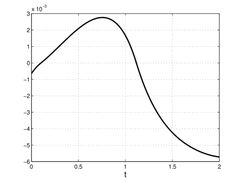
Figure 1: Switching function $m(t)$ in Example 4.

If the set $\{t\in[0,T]:m_{i}(t)=m_{j}(t)\text{ for some }i\not=j\}$ contains isolated points then (11) implies that $u^{*}$ is a bang-bang control corresponding to a switching law in (1). However, in general the optimal control may not be bang-bang. The next result, that follows immediately from Remark 1, describes the relationship between the optimal control problem for the BCCS (II) and the original switched system (1).

Proposition 1

Let $V^{*}:=V(x(T,u^{*}))$. For every $\varepsilon>0$ there exists a piecewise constant switching law $\sigma$ for (1) yielding a cost $V(x(T,\sigma))\leq V^{*}+\varepsilon$. Furthermore, if there exists an optimal control that is piecewise constant and bang-bang then there exists an optimal switching law $\sigma^{*}$ such that $V(x(T,\sigma^{*}))=V^{*}$.

If $\varepsilon_{i}\in\mathbb{R}_{+}$ is a decreasing sequence, with $\lim_{i\to\infty}\epsilon_{i}=0$, then Prop. 1 implies that for every $i$ it is possible to find a switching law $\sigma_{i}$ such that $V(x(T,\sigma_{i}))\leq V^{*}+\varepsilon_{i}$. However, this does not imply that there exists a switching law yielding the optimal cost $V^{*}$, as the limit of a sequence of piecewise constant functions is not necessarily a piecewise constant function.

III-B Geometric considerations

We begin by applying tools from the theory of finite-dimensional Hamiltonian systems to our particular problem. The basic idea is that every symmetry of the Hamiltonian yields a first integral that can be used to simplify the optimal control problem; see [28, Ch. 6]. The Hamiltonian of our optimal control problem is

$$H(x,\lambda):=\lambda^{\prime}\left(\sum_{i=1}^{r}{u_{i}A_{i}}\right)x.$$ (13)

Since $A_{i}$ has zero row sums, $H(x,\lambda)$ is invariant with respect to the translation $x\to x+1_{n}$; the corresponding first integral is $F(x,\lambda):=1_{n}^{\prime}\lambda$. Indeed, $\frac{\partial F}{\partial x}=0$ and $\frac{\partial F}{\partial\lambda}=1_{n}$. Thus, $F(x(t),\lambda(t))$ is a first integral for the Hamiltonian system and this yields the following result.

Proposition 2

The adjoint satisfies

$$1^{\prime}_{n}\lambda(t)=0,\quad\text{for all }t\in[0,T].$$ (14)

Proof:

We already know that $1^{\prime}_{n}\lambda(t)$ is constant, so in particular $1^{\prime}_{n}\lambda(t)\equiv 1_{n}^{\prime}{\lambda}(T)$. Applying (10) yields $1^{\prime}_{n}\lambda(t)\equiv 1^{\prime}_{n}Px^{*}(T)$ and since $1^{\prime}_{n}P=0^{\prime}$, this completes the proof. ∎

The next example demonstrates that for $n=2$ the MP, combined with Prop. 2, can be used to derive (7).

Example 5

Differentiating $m_{i}$ with respect to $t$ and using (II) and (10) yields

$$\dot{m_{i}} =\dot{\lambda}^{\prime}A_{i}x^{*}+\lambda^{\prime}A_{i}\dot{x}^{*}$$

$$=\lambda^{\prime}\left(\sum_{j\neq i}{u_{j}[A_{j},A_{i}]}\right)x^{*}.$$

Suppose that $n=2$. Recall that in this case the matrices can be written as in (4), and a calculation yields

$$[A_{j},A_{i}]=(a_{21}^{i}a_{12}^{j}-a^{i}_{12}a^{j}_{21})\begin{bmatrix}-1&1\\ -1&1\end{bmatrix}.$$

By Prop. 2, $\lambda(t)=\begin{bmatrix}\lambda_{1}(t)&-\lambda_{1}(t)\end{bmatrix}^{\prime}$ for all $t$, so $\dot{m_{i}}(t)\equiv 0$. Thus, for every $i=1,2,\dots,r$,

$$m_{i}(t) \equiv m_{i}(T)$$

$$=\lambda^{\prime}(T)A_{i}x^{*}(T)$$

$$=(x^{*}(T))^{\prime}P^{\prime}A_{i}x^{*}(T)$$

$$=\operatorname{tr}(A_{i})(x_{1}^{*}(T)-x_{2}^{*}(T))^{2}/2.$$ (15)

Assume again that the matrices are ordered as in (6). If $x(0)=c1_{2}$, then the zero sum rows assumption implies that $x_{1}(t)\equiv x_{2}(t)$ for all $u\in\mathcal{U}$, and thus $V(x(T))=0$ for all $u\in\mathcal{U}$. We conclude that in this case every $u\in\mathcal{U}$ is optimal. If $x_{1}(0)\not=x_{2}(0)$ then $x_{1}^{*}(T)\not=x_{2}^{*}(T)$, and combining (5), the fact that $\operatorname{tr}(A_{i})=-a_{12}^{i}-a_{21}^{i}<0$, and (11) yields (7). ∎

Remark 2

Consider the linear consensus system $\dot{x}=Ax$ with $n=2$. Let $0=\eta_{1}\geq\eta_{2}$ denote the eigenvalues of $A$. Recall that the rate of convergence to consensus depends on $\eta_{2}$ (see, e.g., [3]). Since $\operatorname{trace}(A)=\eta_{1}+\eta_{2}=\eta_{2}$, this explains why for $n=2$ the optimal control depends on $\operatorname{sgn}(\operatorname{trace}(A_{i}))$. The optimal control always chooses the matrix with the “better” second eigenvalue. ∎

Example 6

Consider the special case where the matrices also have zero column sums, i.e., $1_{n}^{\prime}A_{i}=0^{\prime}$. It is well-known (see, e.g., [3]) that in this case $\operatorname{Ave}(x(t))$ is invariant, i.e.

$$\operatorname{Ave}(x(t))\equiv\operatorname{Ave}(x_{0}).$$ (16)

Thus, if $\lim_{t\to\infty}x(t)=c1_{n}$ then $c=\operatorname{Ave}(x_{0})$. This is known as average consensus. Let us show that (16) follows from the theory of Hamiltonian symmetry groups; see [28, Ch. 6]. Indeed, in this case the Hamiltonian $H$ in (13) is invariant with respect to the translation $\lambda\to\lambda+1_{n}$; the corresponding first integral is $F(x,\lambda):=1_{n}^{\prime}x$, as $\frac{\partial F}{\partial x}=1_{n}$ and $\frac{\partial F}{\partial\lambda}=0$. Thus, $F(x(t),\lambda(t))$ is a first integral for the Hamiltonian system, so $1_{n}^{\prime}x(t)\equiv 1_{n}^{\prime}x(0)$ and this implies (16). ∎

Remark 3

It is possible to provide an intuitive geometric interpretation of (14). To do this, consider for simplicity the case $n=r=2$. Let $u^{*}$ be an optimal control, and assume for concreteness that

$$x^{*}_{1}(T)>x^{*}_{2}(T),$$ (17)

i.e. $x^{*}(T)$ is “below” the consensus line $l:=\{x\in\mathbb{R}^{2}:x_{1}=x_{2}\}$ (see Fig. 2). Let $\tilde{u}\in\mathcal{U}$ be the control obtained by adding a needle variation, with width $\varepsilon>0$, to $u^{*}$ (as applied in the proof of the PMP), and let $\tilde{x}$ denote the trajectory corresponding to $\tilde{u}$. Let $v$ be the vector such that

$$\tilde{x}(T)-x^{*}(T)=\varepsilon v+o(\varepsilon),$$

i.e. the difference, to first order in $\varepsilon$, between $\tilde{x}(T)$ and $x^{*}(T)$. Let $\mathcal{V}$ denote the set of all these first-order directions for all possible needle variations. Then $\mathcal{V}$ convex, and it is well-known (see e.g. [25, Chapter 4]) that $\lambda(T)$ in the PMP satisfies

$$\lambda^{\prime}(T)v\geq 0,\quad\text{for all }v\in\mathcal{V}.$$

Indeed, the optimality of $u^{*}$ implies that $\mathcal{V}$ cannot span all of $\mathbb{R}^{2}$, and since $\mathcal{V}$ is convex, such a $\lambda(T)$ exists. On the other-hand, (10) yields

$$\lambda(T)=\frac{1}{2}(x_{1}^{*}(T)-x_{2}^{*}(T))\begin{bmatrix}1\\ -1\end{bmatrix},$$

and using (17) implies that $\lambda(T)$ is as shown in Fig. 2. In other words, $\lambda(T)$ is a normal to the line $l$ and the MP states that $\tilde{x}(T)$ cannot be closer to the “consensus line” $l$ than $x^{*}(T)$. ∎

More generally, recall that for $y\in\mathbb{R}^{n}$ the disagreement vector of $y$ is defined by $\delta(y):=y-1_{n}\operatorname{Ave}(y)$ (see, e.g., [3]). By the definition of $P$, $Py=\delta(y)$ for all $y$, and it follows from (10) that $\lambda(T)=\delta(x^{*}(T)).$ Thus, the geometric interpretation of the MP is that any needle perturbation of $u^{*}$ cannot lead to a value $\tilde{x}(T)$ that is closer to the consensus hyperplane $\{x\in\mathbb{R}^{n}:x_{1}=\dots=x_{n}\}$ than $x^{*}(T)$.

Note also that since $P=P^{\prime}P$,

$$V(x(t)) =x^{\prime}(t)P^{\prime}Px(t)$$

$$=\delta^{\prime}(t)\delta(t).$$

Figure 2: Geometric interpretation of Prop. 2 when $n=2$. The vector $v$ is $\tilde{x}(T)-x^{*}(T)$, to first-order in $\varepsilon$, and its inner product with $\lambda(T)$ must be non-negative.

III-C Invariance with Respect to Permutations

Let $\Sigma$ denote the set of all $n\times n$ permutation matrices. Fix an arbitrary $G\in\Sigma$, and define $\tilde{x}(t,u)=Gx(t,u)$. The dynamics for the $\tilde{x}$ system is given by

$$\dot{\tilde{x}} =G(\sum_{i=1}^{r}u_{i}A_{i})G^{\prime}\tilde{x},$$

$$\tilde{x}(0) =Gx_{0}.$$ (18)

Proposition 3

A control $u^{*}$ is an optimal control for (II) if and only if it is an optimal control for (III-C).

Proof:

Note that

$$G^{\prime}PG =G^{\prime}(I-(1/n)1_{n}1^{\prime}_{n})G$$

$$=I-(1/n)G^{\prime}1_{n}1^{\prime}_{n}G$$

$$=I-(1/n)1_{n}1^{\prime}_{n}$$

$$=P.$$

Now fix an arbitrary control $u\in\mathcal{U}$ and let $x(t,u)$ denote the corresponding solution of (II) at time $t$. Define $\tilde{x}(t,u)=Gx(t,u)$. Then

$$V(\tilde{x}(t,u)) =\tilde{x}^{\prime}(t,u)P\tilde{x}(t,u)$$

$$=x^{\prime}(t,u)G^{\prime}PGx(t,u)$$

$$=V(x(t,u)).$$

This implies that a control $u^{*}$ is an optimal control for (II) if and only if it is an optimal control for the $\tilde{x}$ system given by (III-C) and $V(x(t,u^{*}))=V(\tilde{x}(t,u^{*}))$ for all $t\in[0,T]$. ∎

III-D Dimension reduction

It is well-known that the special structure of the consensus matrix allows a dimension reduction to the $(n-1)$-dimensional subspace $\{c1_{n}:c\in\mathbb{R}\}^{\perp}$ (see, e.g., [3, 29, 30]). Here we apply this idea to reduce the dimension of the optimal control problem.

Note that $s^{1}:=1_{n}$ is an eigenvector of $P$ corresponding to the eigenvalue $0$. Furthermore, any vector with sum entries equal to zero is an eigenvector of $P$ corresponding to the eigenvalue $1$. This implies that there exists a set of $n$ linearly independent vectors $\{s^{1},s^{2},\dots,s^{n}\}$, with $s^{k}\in\mathbb{R}^{n}$, satisfying: (1) $Ps^{1}=0$; and (2) $Ps^{k}=s^{k}$, $k=2,\dots,n$. Let

$$S:=\begin{bmatrix}s^{1}&s^{2}&\dots&s^{n}\end{bmatrix}^{\prime}$$

(note the transpose here). We use $S$ to reduce the order of the bilinear control system.

Proposition 4

Fix an arbitrary control $u\in\mathcal{U}$. Let $x(t)$ denote the solution of (II) at time $t$. Define $y:[0,T]\to\mathbb{R}^{n}$ and $z:[0,T]\to\mathbb{R}^{n-1}$ by

$$y(t):=Sx(t),\quad z(t):=Ry(t),$$

where $R\in\mathbb{R}^{(n-1)\times n}$ is the matrix

$$R:=\begin{bmatrix}0&1&0&\cdots&0\\ 0&0&1&\cdots&0\\ \vdots&&&\ddots\\ 0&0&0&\dots&1\\ \end{bmatrix}.$$

Then $z$ satisfies

$$\dot{z}=\left(\sum_{i=1}^{r}{u_{i}\bar{A}_{i}}\right)z,\quad z(0)=RSx_{0},$$ (19)

where $\bar{A}_{i}\in\mathbb{R}^{(n-1)\times(n-1)}$ is the matrix obtained by deleting the first row and the first column of $SA_{i}S^{-1}$. Furthermore, there exists a positive-definite matrix $M\in\mathbb{R}^{(n-1)\times(n-1)}$ such that

$$V(x(t))=z^{\prime}(t)Mz(t),\quad\text{for all }t\geq 0,$$ (20)

Remark 4

Let $\|x\|_{M}:=\sqrt{x^{\prime}Mx}$. Prop. 4 implies that the original optimal control problem, namely, $\min_{u\in\mathcal{U}}V(x(T,u))$ becomes, in the $z$-coordinates, the $(n-1)$-dimensional optimal control problem $\min_{u\in\mathcal{U}}\|z(T,u)\|_{M}^{2}$. However, in the bilinear dynamics of $\dot{z}$ given in (19) the matrices are not necessarily Metzler, nor with zero sum rows. This implies in particular that the switched consensus system is UCC if and only if the reduced-order $z$ system is GUAS. ∎

Proof:

It is straightforward to verify that the first column of $S^{-1}$ is a multiple of $1_{n}$. Since

$$\dot{y}=\left(\sum_{i=1}^{r}{u_{i}SA_{i}S^{-1}}\right)y,$$ (21)

and the first column of $SA_{i}S^{-1}$ is zero, $\dot{y}_{2},\dots,\dot{y}_{n}$ do not depend on $y_{1}$, i.e. the dynamics of the $z_{i}$s is given by the $(n-1)$-dimensional bilinear control system (19). Furthermore,

$$V(x) =x^{\prime}Px$$

$$=y^{\prime}(S^{-1})^{\prime}PS^{-1}y.$$

Since $P1_{n}=0$ and $1_{n}^{\prime}P=0^{\prime}$, both the first column and the first row of $(S^{-1})^{\prime}PS^{-1}$ are zero, so $V(x)=\begin{bmatrix}0&z^{\prime}\end{bmatrix}(S^{-1})^{\prime}PS^{-1}\begin{bmatrix}0\\ z\end{bmatrix}=z^{\prime}Mz$, with $M:=R(S^{-1})^{\prime}PS^{-1}R^{\prime}$. A straightforward calculation shows that $(S^{-1})^{\prime}PS^{-1}v=0$ holds (up to a multiplication by a scalar) only for $v=S1_{n}$, so $M>0$. ∎

Example 7

Consider the case $n=2$. Recall that in this case $A_{i}$ has the form (4). Take $s^{1}=\begin{bmatrix}1&1\end{bmatrix}^{\prime}$, $s^{2}=\begin{bmatrix}1&-1\end{bmatrix}^{\prime}$. Then $SA_{i}S^{-1}=\begin{bmatrix}0&a^{i}_{21}-a^{i}_{12}\\ 0&-(a^{i}_{12}+a^{i}_{21})\end{bmatrix}$, so $\bar{A}_{i}=-(a^{i}_{12}+a^{i}_{21})$. Also, $M=1/2$, so $V(z)=z^{2}/2$. Thus, the dimension reduction argument yields a trivial problem of switching between $r$ one-dimensional subsystems with eigenvalues $-(a^{i}_{12}+a^{i}_{21})=\operatorname{tr}(A_{i})$. ∎

Example 8

Consider the case $n=3$. Then the matrices may be written as

$$A_{i}=\begin{bmatrix}-a^{i}_{12}-a^{i}_{13}&a^{i}_{12}&a^{i}_{13}\\ a^{i}_{21}&-a^{i}_{21}-a^{i}_{23}&a^{i}_{23}\\ a^{i}_{31}&a^{i}_{32}&-a^{i}_{31}-a^{i}_{32}\end{bmatrix},$$ (22)

with $a^{i}_{kj}\geq 0$. Take $s^{1}=\begin{bmatrix}1&1&1\end{bmatrix}^{\prime}$, $s^{2}=\begin{bmatrix}1&-1&0\end{bmatrix}^{\prime}$, and $s^{3}=\begin{bmatrix}0&1&-1\end{bmatrix}^{\prime}$. Then a calculation yields

$$SA_{i}S^{-1}=\begin{bmatrix}0&*&*\\ 0&\bar{a}_{11}^{i}&\bar{a}_{12}^{i}\\ 0&\bar{a}_{21}^{i}&\bar{a}_{22}^{i}\end{bmatrix},$$ (23)

where $*$ denotes entries that are not important for the derivations below, and

$$\bar{a}_{11}^{i} =-({a^{i}_{12}}+{a^{i}_{13}}+{a^{i}_{21}}), \quad\bar{a}_{12}^{i} =a^{i}_{23}-a^{i}_{13},$$ (24)

$$\bar{a}_{21}^{i} ={a^{i}_{21}}-{a^{i}_{31}}, \quad\bar{a}_{22}^{i} =-({a^{i}_{23}}+{a^{i}_{31}}+{a^{i}_{32}}).$$

Clearly, the dynamics of $y_{2}(t)$ and $y_{3}(t)$ does not depend on $y_{1}(t)$, and the $z$ dynamics depends on

$$\bar{A}_{i}:=\begin{bmatrix}\bar{a}_{11}^{i}&\bar{a}_{12}^{i}\\ \bar{a}_{21}^{i}&\bar{a}_{22}^{i}\end{bmatrix},\quad i=1,\dots,r.$$ (25)

Also,

$$M=R(S^{-1})^{\prime}PS^{-1}R^{\prime}=\frac{1}{3}\begin{bmatrix}2&1\\ 1&2\end{bmatrix}.$$ (26)

∎

The next result shows how the dimension reduction allows to reduce the order of the optimal control problem from $2n$ to $2n-2$ (cf. [28, Ch. 6]).

Proposition 5

Let $u^{*}\in\mathcal{U}$ be an optimal control for Problem 3, and let $z^{*}$ denote the corresponding trajectory of the $(n-1)$-dimensional system (19). Define $\mu:[0,T]\to\mathbb{R}^{n-1}$ by

$$\dot{\mu}(t)=-\left(\sum_{i=1}^{r}{u_{i}^{*}\bar{A}_{i}}\right)^{\prime}\mu(t),\;\mu(T)=R(S^{-1})^{\prime}PS^{-1}R^{\prime}z^{*}(T),$$ (27)

and let $\bar{m}_{i}(t):=\mu^{\prime}(t)\bar{A}_{i}z^{*}(t)$. Then for almost all $t\in[0,T]$, if $\bar{m}_{i}(t)>\bar{m}_{j}(t)$ for every $j\neq i$, then

$$u_{i}^{*}(t)=0.$$ (28)

Proof:

Let $\gamma(t):=(S^{-1})^{\prime}\lambda(t)$, where $\lambda(t)$ satisfies (10). Then

$$\dot{\gamma}(t)=-\left(\sum_{i=1}^{r}u_{i}^{*}S{A}_{i}S^{-1}\right)^{\prime}\gamma(t),\;\gamma(T)=(S^{-1})^{\prime}PS^{-1}y^{*}(T).$$

The definition of $\gamma$ and Prop. 2 imply that $\gamma_{1}(t)\equiv 0$, so letting $\mu(t):=R\gamma(t)$ yields (27). Also $m_{i}(t)=\gamma^{\prime}(t)SA_{i}S^{-1}y^{*}(t)=\mu^{\prime}(t)\bar{A}_{i}z^{*}(t)$. Combining this with Thm. 1 completes the proof. ∎

III-E The case $n=3$ and $r=2$

Consider a switched consensus system with $n=3$ and $r=2$. Recall that in this case the dimensionality reduction yields a switched system with dimension $n=2$ and $r=2$. Second-order linear switched systems have been studied extensively and many explicit results are known, especially when the number of subsystems is $r=2$. Using this, we derive two results. The first is a necessary and sufficient condition for UCC. The second is a characterization of an optimal control.

III-E1 Convergence to consensus

Recall that we can associate with $\dot{x}=Ax$, where $A\in\mathbb{R}^{n\times n}$ is a consensus matrix, a directed and weighted graph $G=(V,E,W)$, where $V=\{1,\dots,n\}$, and there is a directed edge from node $i$ to node $j\not=i$, with weight $w_{ji}=a_{ji}$, if and only if $a_{ji}\not=0$. The graph $G$ is said to contain a rooted-out branching as a subgraph if it does not contain a directed cycle and there exists a vertex $v$ (called the root) such that for every vertex $p\in V\setminus\{v\}$ there is a directed path from $v$ to $p$. A necessary and sufficient condition for containing a rooted-out branching is that $\operatorname{rank}(A)=n-1$ [2, Ch. 3].

For two matrices $A,B\in\mathbb{R}^{n\times n}$, let $\operatorname{co}[A,B]:=\{\alpha A+(1-\alpha)B:\;\alpha\in[0,1]\}.$

Theorem 2

The switched consensus system (1) with $n=3$ and $r=2$ is UCC if and only if the digraph corresponding to every matrix in $\operatorname{co}[A_{1},A_{2}]$ contains a rooted-out branching.

Proof:

Assume that the digraph corresponding to $\alpha A_{1}+(1-\alpha)A_{2}$ does not contain a rooted-out branching for some $\alpha\in[0,1]$. Then the solution of the BCCS (II) with $u_{1}(t)\equiv\alpha$ does not converge to consensus for some $x_{0}\in\mathbb{R}^{3}$, and by Remark 1, there is a solution of the switched consensus system (1) that does not converge to consensus.

To prove the converse implication, assume from here on that the digraph corresponding to every matrix in $\operatorname{co}[A_{1},A_{2}]$ contains a rooted-out branching, so the rank of every matrix is $2$. We will show that in this case the reduced order $z$ system is GUAS. We require the following result.

Theorem 3

[31] Let $Z_{1},Z_{2}\in\mathbb{R}^{2\times 2}$ be two Hurwitz matrices. There exists a matrix $Y>0$ such that

$$YZ_{i}+Z_{i}^{\prime}Y<0,\quad i=1,2,$$ (29)

if and only if every matrix in $\operatorname{co}[Z_{1},Z_{2}]$ and in $\operatorname{co}[Z_{1},Z_{2}^{-1}]$ is a Hurwitz matrix.

Note that condition (29) implies that $Q(x):=x^{\prime}Yx$ is a common quadratic Lyapunov function (CQLF) for both $\dot{x}=Z_{1}x$ and $\dot{x}=Z_{2}x$.

Thus, to prove GUAS of the second-order $z$ system it is enough to show that

$$\operatorname{co}[\bar{A}_{1},\bar{A}_{2}]\text{ is Hurwitz},$$ (30)

and

$$\operatorname{co}[\bar{A}_{1},\bar{A}_{2}^{-1}]\text{ is Hurwitz}.$$ (31)

A calculation yields

$$\bar{t}_{i} :=\operatorname{tr}(\bar{A}_{i})=-(a_{12}^{i}+a_{13}^{i}+a_{21}^{i}+a_{23}^{i}+a_{31}^{i}+a_{32}^{i}),$$

$$\bar{d}_{i} :=\det(\bar{A}_{i})=(a_{21}^{i}+a_{23}^{i})(a_{13}^{i}+a_{31}^{i})+(a_{13}^{i}+a_{21}^{i})a_{32}^{i}$$

$$+a_{12}^{i}(a_{23}^{i}+a_{31}^{i}+a_{32}^{i}).$$

This implies that $\bar{t}_{i}\leq 0$, with equality if and only if $A_{i}=0$. Also, $\bar{d}_{i}\geq 0$ with equality if and only if $\operatorname{rank}(A_{i})<2$.

Pick $\alpha\in[0,1]$. By assumption, $\operatorname{rank}(\alpha A_{1}+(1-\alpha)A_{2})=2$, so $\det(\alpha\bar{A}_{1}+(1-\alpha)\bar{A}_{2})>0$, and $\operatorname{tr}(\alpha\bar{A}_{1}+(1-\alpha)\bar{A}_{2})=\alpha\bar{t}_{1}+(1-\alpha)\bar{t}_{2}<0$. Thus, (30) holds.

To prove (31), let $M:=\alpha\bar{A}_{1}+(1-\alpha)\bar{A}_{2}^{-1}$. Seeking a contradiction, assume that $\det(M)=0$. Then clearly $\alpha\not=1$. Also, there exists $v\in\mathbb{R}^{2}\setminus\{0\}$ such that $\alpha\bar{A}_{2}\bar{A}_{1}v=-(1-\alpha)v$. This implies that $\alpha\not=0$, so $\bar{A}_{2}\bar{A}_{1}$ has a real and negative eigenvalue. Since $\det(\bar{A}_{2}\bar{A}_{1})=\bar{d}_{1}\bar{d}_{2}>0$, $\bar{A}_{2}\bar{A}_{1}$ has two negative eigenvalues. However, a calculation shows that $\operatorname{tr}(\bar{A}_{2}\bar{A}_{1})$ is the sum of terms in the form $a^{1}_{ij}a^{2}_{kl}$ and thus $\operatorname{tr}(\bar{A}_{2}\bar{A}_{1})\geq 0$. This contradicts the conclusion that $\bar{A}_{2}\bar{A}_{1}$ has two negative eigenvalues. Thus, $\det(M)\not=0$ and therefore

$$\det(\alpha\bar{A}_{1}+(1-\alpha)\bar{A}_{2}^{-1})>0,\quad\text{ for all }\alpha\in[0,1].$$

We now turn to consider $\bar{q}:=\operatorname{tr}(\alpha\bar{A}_{1}+(1-\alpha)\bar{A}_{2}^{-1})$. Since the matrices are $2\times 2$, $q=\alpha\bar{t}_{1}+(1-\alpha)\bar{t}_{2}/\bar{d}_{2}$. Since $\bar{t}_{i}<0$ and $\bar{d}_{2}>0$, $\bar{q}<0$. This proves (31). Thus, the reduced-order switched system admits a CQLF and thus it is GUAS. By Remark 4, the switched consensus system is UCC. ∎

Example 9

Consider again the matrices in Example 2. Here it is straightforward to see that $\operatorname{rank}(\operatorname{co}[A_{1},A_{2}])=2$. In this case (23) yields $\bar{A}_{1}=\begin{bmatrix}-5&0\\ 2&-0.01\end{bmatrix}$, and $\bar{A}_{2}=\begin{bmatrix}-3&0\\ 1&-0.1\end{bmatrix}$. These two matrices clearly admit a CQLF. For example, for $Y:=\begin{bmatrix}100&0\\ 0&4\end{bmatrix}$, we have $Q_{1}:=-(Y\bar{A}_{1}+\bar{A}_{1}^{\prime}Y)=\begin{bmatrix}1000&-8\\ -8&0.08\end{bmatrix}>0$, and $Q_{2}:=-(Y\bar{A}_{2}+\bar{A}_{2}^{\prime}Y)=\begin{bmatrix}600&-4\\ -4&0.8\end{bmatrix}>0$. We note in passing that combining this with Remark 4 can be used to obtain an explicit exponential upper bound on the rate of convergence to consensus for arbitrary switching laws. ∎

III-E2 Nice optimality

One may intuitively expect that every optimal control will be “nice” or “regular” in some sense. This expectation is wrong. Indeed, we already saw in Example 1 that there are cases where every control $u\in\mathcal{U}$ is optimal. A more reasonable expectation (at least in some cases) is that there always exists at least one optimal control that is “nice”. This kind of nice-optimality results are important because they imply that the search for an optimal control may be limited to a subset of “nice” controls that may be much smaller than $\mathcal{U}$. A classic example is the bang-bang theorem stating that for linear control systems there always exists an optimal control that is piecewise-constant and bang-bang (see, e.g. [32]).

We introduce some notation for scalar controls. Given two controls $u_{1}:[0,T_{1}]\to[0,1]$ and $u_{2}:[0,T_{2}]\to[0,1]$, let $u_{2}*u_{1}$ denote their time-concatenation, that is,

$$(u_{2}*u_{1})(t):=\begin{cases}u_{1}(t),&t\in[0,T_{1}),\\ u_{2}(t-T_{1}),&t\in[T_{1},T_{1}+T_{2}].\end{cases}$$

The corresponding trajectory $x:[0,T_{1}+T_{2}]\to\mathbb{R}^{n}$ is obtained by first following $u_{1}$ and then $u_{2}$. For $\mathcal{U}_{1},\mathcal{U}_{2}\subseteq\mathcal{U}$, let $\mathcal{U}_{2}*\mathcal{U}_{1}$ denote the set of all concatenations $u_{2}*u_{1}$ where, for $i=1,2$, either $u_{i}\in\mathcal{U}_{i}$ or $u_{i}$ is trivial (that is, the domain of $u_{i}$ includes a single point). Hence, $\mathcal{U}_{2}*\mathcal{U}_{1}$ essentially contains both $\mathcal{U}_{1}$ and $\mathcal{U}_{2}$ themselves. For example, if $\mathcal{B}_{k}\subset\mathcal{U}$ denotes the set of piecewise constant bang-bang controls with no more than $k$ discontinuities, then $(\mathcal{B}_{1}*\mathcal{B}_{2})=\mathcal{B}_{4}$ (as the concatenation may introduce an additional discontinuity).

Consider a bang-bang control $u:\mathbb{R}_{+}\to[0,1]$ with switching times $T_{1}<T_{2}<T_{3}<\dots$, that is, $u(t)=v$ for $t\in[0,T_{1})$, $u(t)=1-v$ for $t\in[T_{1},T_{2})$, and so on where $v\in\{0,1\}$. Denote $T_{ij}:=T_{i}-T_{j}$. We say that $u$ is periodic after three switches if $T_{21}=T_{43}=T_{65}=\dots$ and $T_{32}=T_{54}=T_{76}=\dots$. Let $\mathcal{B}\mathcal{P}\subset\mathcal{U}$ denote the set of such controls, and let $\mathcal{P}\mathcal{C}_{k}\subset\mathcal{U}$ denote the set of piecewise constant functions with no more than $k$ discontinuities. Let

$$\mathcal{W}:=(\mathcal{B}_{0}*\mathcal{B}\mathcal{P})\cup(\mathcal{B}_{0}*\mathcal{P}\mathcal{C}_{2}),$$

i.e. the union of: (1) controls that are a concatenation of a control that is periodic after three switches and a bang arc; and (2) controls that are a concatenation of a piecewise constant control with no more than two discontinuities and a bang arc.

We can now state our second main result in this subsection.

Theorem 4

Suppose that $n=3$ and $r=2$. Fix arbitrary $x_{0}\in\mathbb{R}^{3}$ and $T\geq 0$. Consider Problem 3. There exists an optimal control $u^{*}=\begin{bmatrix}u^{*}_{1}&1-u^{*}_{1}\end{bmatrix}^{\prime}$ satisfying

$$u^{*}_{1}\in\mathcal{W}.$$ (32)

Proof:

When $n=3$ the reduced-order $z$-system is a planar bilinear control system. It was shown in [33] that the reachable set of a planar bilinear control system with $r=2$ satisfies

$$R(T,\mathcal{U},x_{0})=R(T,\mathcal{W},x_{0}),\;\;\text{for all }x_{0}\in\mathbb{R}^{2}\text{ and all }T\geq 0.$$ (33)

This implies of course that we can find an optimal control $u^{*}$ for the the $z$-system satisfying $u^{*}\in\mathcal{W}$. By Remark 4, this control is also an optimal control for the original bilinear control system. ∎

Recall that a set $C\subseteq\mathbb{R}^{n}$ is called a convex cone if $p,q\in C$ implies that $k_{1}p+k_{2}q\in C$ for all $k_{1},k_{2}\geq 0$. The cone is said to be: solid if its interior is non-empty; pointed if $C\cap(-C)=\{0\}$; proper if it is both solid and pointed. It was shown in [33] that if there exists a proper cone $C\subset\mathbb{R}^{2}$ that is an invariant set of the planar bilinear dynamics then (33) can be strengthened to

$$R(T,\mathcal{U},x_{0})=R(T,\mathcal{V},x_{0}),\;\;\text{for all }x_{0}\in\mathbb{R}^{2}\text{ and all }T\geq 0,$$

where $\mathcal{V}:=\mathcal{B}_{3}\cup(\mathcal{B}_{0}*\mathcal{P}\mathcal{C}_{2})$. Since the $A_{i}$s are Metzler, the BCCS admits the proper cone $\mathbb{R}_{+}^{3}$ as an invariant set. Thus, $\{Sx:x\in\mathbb{R}^{3}_{+}\}$ is an invariant set of the $y$ system, and

$$\left\{\begin{bmatrix}0&1&0\\ 0&0&1\end{bmatrix}Sx:x\in\mathbb{R}^{3}_{+}\right\}\subseteq\mathbb{R}^{2}$$

is an invariant set of the $z$ system. However, this set is not a proper cone in $\mathbb{R}^{2}$, as it is not pointed.

III-F Worst-case analysis

We convert Problem 2 into the following optimal control problem.

Problem 4

Given the bilinear consensus system (II) and a final time $T>0$, find a control $v^{*}\in\mathcal{U}$ that maximizes $V(x(T))$.

Intuitively, $v^{*}$ maximizes the distance to consensus, so it is a worst-case control.

Since

$$\max_{v\in\mathcal{U}}V(x(T)) =\min_{v\in\mathcal{U}}(-V(x(T)))$$ (34)

$$=\min_{v\in\mathcal{U}}x^{\prime}(T)(-P)x(T),$$

all the results about the optimal control derived above hold once $P$ is replaced with $-P$. For example, the MP in Thm. 1 becomes a necessary condition for the optimality of $v^{*}$ once (10) is replaced by

$$\dot{\lambda}(t)=-\left(\sum_{i=1}^{r}{u_{i}^{*}A_{i}}\right)^{\prime}\lambda(t),\quad\lambda(T)=(-P)x^{*}(T).$$ (35)

Example 10

Consider again the matrices $A_{1},A_{2}$ in Example 2 with $T=1$ and $x_{0}=\begin{bmatrix}1&2&1\end{bmatrix}^{\prime}$. Using a simple numerical algorithm for determining the worst-case control yields

$$v^{*}(t)=\begin{cases}1,&t\in[0,\tau),\\ 0,&t\in(\tau,1],\end{cases}$$ (36)

where $\tau\approx 0.346429$. The corresponding trajectory is

$$x^{*}(T) =\exp(A_{1}(T-\tau))\exp(A_{2}\tau)x_{0}$$

$$=\begin{bmatrix}1.635003&1.648475&1.034004\end{bmatrix}^{\prime}$$

and $V(x^{*}(T))=0.246319$. On the other hand, if we use only one of the subsystems then we get either

$$\exp(A_{1}T)x_{0} =\begin{bmatrix}1.595957&1.602695&1.006758\end{bmatrix}^{\prime},$$

$$V(\exp(A_{1}T)x_{0}) =0.234114,$$

or

$$\exp(A_{2}T)x_{0} =\begin{bmatrix}1.633475&1.683262&1.073270\end{bmatrix}^{\prime},$$

$$V(\exp(A_{2}T)x_{0}) =0.229467.$$

Thus, in this case the switching indeed strictly slows down the convergence to consensus at the final time $T$. Given $v^{*}$, it is straightforward to compute the adjoint in (35) and the switching function $m(t)$ (see Fig. 3). It may be seen that $m(t)<0$ for $t\in[0,\tau)$, and $m(t)>0$ for $t\in(\tau,T]$. Thus, $u^{*}$ indeed satisfies (11). ∎

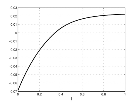
Figure 3: Switching function $m(t)$ in Example 10.

In the reduced-order system, the maximization problem (34) becomes

$$\max_{u\in\mathcal{U}}\|z(T,u)\|_{M}^{2},$$ (37)

where $z$ satisfies (19). Recall that this is an $(n-1)$-dimensional problem. Furthermore, this problem is also closely related to the GUAS problem. Indeed, let $v^{*}\in\mathcal{U}$ be a solution to (37). Then $v^{*}$ “pushes” the state $z$ as far as possible from the origin (for the given final time $T$, initial condition $z_{0}=RSx_{0}$, and metric $\|\cdot\|_{M}$). Since GUAS means convergence to the origin for any control, $v^{*}$ may be interpreted as the “most destabilizing” control (see [30, 29] for closely related ideas in the context of discrete-time consensus algorithms). In the remainder of this section, we explore some of the implications of this connection.

We already know that when $n=2$ there always exists an optimal control $u^{*}$ for Problem 3 that is bang-bang with no switches. The same holds for Problem 4. The next example shows that for $n=3$ this is no longer true.

Example 11

Consider Problem 4 with $n=3$, $r=2$, $T=1$,

$$A_{1}=\begin{bmatrix}-1&1&0\\ 0&-1&1\\ 0&0&0\end{bmatrix},\quad A_{2}=\begin{bmatrix}0&0&0\\ 1&-1&0\\ 0&1&-1\end{bmatrix},$$

and $x_{0}=\begin{bmatrix}2&1&0\end{bmatrix}^{\prime}$. The corresponding BCCS is given by $\dot{x}=(A+Bu)x$, with $u(t)\in[0,1]$, $A:=A_{1}$ and $B:=A_{2}-A_{1}$. We claim that no bang-bang control is optimal. To prove this, assume that $v^{*}$ is an optimal control that is bang-bang. The reduced-order system is $\dot{z}=(\bar{A}+\bar{B}u)z$, with $\bar{A}=\begin{bmatrix}-1&1\\ 0&-1\end{bmatrix}$, $\bar{B}=\begin{bmatrix}0&-1\\ 1&0\end{bmatrix}$, $z_{0}=\begin{bmatrix}1&1\end{bmatrix}^{\prime}$. We know that $v^{*}$ maximizes $|z(T,u)|_{M}^{2}$, with $M$ given in (26), i.e., $|z(1,v^{*})|_{M}^{2}=\max_{u\in\mathcal{U}}|z(1,u)|_{M}^{2}$. The reduced-order system is a positive bilinear control system, as both $\bar{A}$ and $\bar{A}+\bar{B}$ are Metzler matrices. Thus, $\mathbb{R}^{2}_{+}$ is an invariant cone of the dynamics and by [33, Thm. 2], $v^{*}$ has no more than two switches. In other words, the corresponding trajectory satisfies either

$$z^{*}(1)=\exp(\bar{A}(1-t_{1}-t_{2}))\exp((\bar{A}+\bar{B})t_{2})\exp(\bar{A}t_{1})z_{0},$$

or

$$z^{*}(1)=\exp((\bar{A}+\bar{B})(1-t_{1}-t_{2}))\exp(\bar{A}t_{2})\exp((\bar{A}+\bar{B})t_{1})z_{0},$$

where

$$t_{1},t_{2}\geq 0,\quad t_{1}+t_{2}\leq 1.$$ (38)

Since $\bar{A},\bar{A}+\bar{B}\in\mathbb{R}^{2\times 2}$ and both are triangular, it is straightforward to show that both possible forms yield

$$|z^{*} (1)|^{2}_{M}=(2(7+t_{2}(4+(4-5t_{1})t_{1}-4t_{2}$$

$$+t_{1}(-3+(t_{1}-1)t_{1}^{2})t_{2}+(t_{1}^{2}-1)(1+2t_{1})t_{2}^{2}$$

$$+(1+t_{1})^{2}t_{2}^{3})))/(3\exp(2)).$$

Maximizing this subject to (38) yields $t_{1}^{*}\approx 0.2570$, $t_{2}^{*}\approx 0.4615$, and

$$|z^{*}(1)|^{2}_{M}\approx 0.72918.$$ (39)

On the other hand, the control $u(t)\equiv 1/2$ yields

$$z(1) =\exp(\bar{A}+\bar{B}/2)z_{0}$$

$$=\exp(-1/2)\begin{bmatrix}1&1\end{bmatrix}^{\prime},$$

so $|z(1)|^{2}_{M}=2\exp(-1)\approx 0.73576.$ Comparing this to (39) implies that $v^{*}$ is not optimal, so there is no optimal control that is bang bang. In fact, the control $u(t)\equiv 1/2$ is an optimal control. To explain this, note that the eigenvalues of the matrices $\bar{A}_{1},\bar{A}_{2}$ are $\{-1,-1\}$, so the speed of convergence to consensus obtained by using each matrix is $\exp(-t)$. However, the eigenvalues of the matrix $(\bar{A}_{1}+\bar{A}_{2})/2$ (that corresponds to $u(t)\equiv 1/2$) are $\{-1/2,-3/2\}$, where $-1/2$ corresponds to the eigenvector $z_{0}=\begin{bmatrix}1&1\end{bmatrix}^{\prime}$. Thus, for $z(0)=z_{0}$, the rate of convergence to consensus is $\exp(-t/2)$, which is of course slower than $\exp(-t)$ (recall that we are considering the problem of maximizing $V(x(T,u))$). ∎

In general, it is possible of course that a switched system, composed of two asymptotically stable subsystems, will have a diverging trajectory for some switching law. For the reduced-order problem derived from the consensus problem this is not the case, as every trajectory of (19) is bounded. This follows from the fact [20] that $\tilde{V}(x):=\max_{i\in\{1,\dots,n\}}x_{i}-\min_{i\in\{1,\dots,n\}}x_{i}$ is non-increasing along the solution of every linear consensus system (see also [35] for some related considerations). Letting $Q\in\mathbb{R}^{n\times(n-1)}$ denote the matrix $S^{-1}$ with its first column deleted, and using $x=S^{-1}y$, and the fact that the first column of $S^{-1}$ is $c1_{n}$, $c\in\mathbb{R}$, yields

$$x =c{y_{1}}1_{n}+Q\begin{bmatrix}y_{2}&\dots&y_{n}\end{bmatrix}^{\prime}$$

$$=c{y_{1}}1_{n}+Qz.$$

Thus, $\tilde{V}(x(t))\equiv\tilde{W}(z(t))$, where

$$\tilde{W}(z):=\max_{i\in\{1,\dots,n\}}(Qz)_{i}-\min_{i\in\{1,\dots,n\}}(Qz)_{i}.$$

This implies that $\tilde{W}(z(t))$ remains bounded along solutions of the reduced-order system, and since the columns of $Q$ are linearly independent, this implies that every trajectory is bounded.

Example 12

Consider again the system in Example 10. Recall that the worst case control is given in (36). Let $z^{*}$ denote the corresponding trajectory of the reduced-order system. The function $\tilde{W}(z^{*}(t))$ is depicted in Fig. 4. It may be seen that $\tilde{W}(z^{*}(t))$ remains bounded (in fact, it is strictly decreasing). Note the change in the dynamics at the switching point $\tau\approx 0.35$. ∎

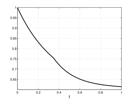
Figure 4: Function $\tilde{W}(z^{*}(t))$ in Example 10.

IV Discussion

Consensus algorithms are essential building blocks in distributed systems. In these systems, the possibility to exchange local information between the agents may be time-varying. A standard model for this is a switched system, switching between several subsystems, each implementing a consensus algorithm with a different connectivity pattern.

In the continuous-time linear case, each subsystem is in the form $\dot{x}=A_{i}x$, where $A_{i}$ is a Metzler matrix with zero row sums. The switching law may have a strong effect on the convergence to consensus and a natural problem is: find a best (or worst) possible switching law.

We consider this question in the framework of optimal control theory. This is motivated by the variational approach used to analyze the GUAS problem in switched systems. In particular, in the case of positive linear switched systems (PLSSs) each subsystem is in the form $\dot{x}=A_{i}x$, with $A_{i}$ a Metzler matrix (see e.g. [8, 9]). Recently, the variational approach was extended to address the GUAS problem for PLSSs [36]. Here the optimality criterion is maximizing the spectral radius of the transition matrix [36].

One advantage of this variational approach is that it allows bringing to bear powerful techniques from optimal and geometric control theory. We apply the PMP to obtain a necessary condition for optimality. The special structure of the consensus problem allows a dimensionality reduction. This shows that a switched consensus system is UCC if and only if a reduced order linear switched system is GUAS. One application of this is that computational complexity results for the GUAS problem (see, e.g. [37, 38]) immediately imply similar results for the UCC problem.

The variational approach leads to a complete solution of the problem when the dimension is $n=2$. For the case $n=3$, and $r=2$, we show that there always exists an optimal control that is “nice”. We also show that the switched consensus system is UCC if and only if the digraph corresponding to any matrix in the convex hull of the two subsystems has a rooted-out branching.

The variational approach has also been used to analyze the GUAS problem for nonlinear switched systems [39, 40, 41], and for discrete-time switched systems [42, 43]. Extensions of the approach described here to nonlinear consensus algorithms [44], and to discrete-time consensus problems [21] may thus be possible.

Finally, note that combining the MP with efficient numerical algorithms for solving optimal control problems may lead to explicit numerical lower and upper bounds for the convergence rate to consensus in many real-world problems. Any algorithm for determining the switching between the subsystems, including those that are based on local information only, can be rated by comparing them to these bounds.

References

- [1] O. Ron and M. Margaliot, “Optimal switching between two linear consensus protocols,” in Proc. 52nd IEEE Conf. on Decision and Control, Florence, Italy, 2013.
- [2] M. Mesbahi and M. Egerstedt, Graph Theoretic Methods in Multiagent Networks. Princeton University Press, 2010.
- [3] R. Olfati-Saber and R. M. Murray, “Consensus problems in networks of agents with switching topology and time-delays,” IEEE Trans. Automat. Control, vol. 49, pp. 1520–1533, 2004.
- [4] D. Zelazo, M. Burger, and F. Allgower, “Dynamic negotiation under switching communication,” in Mathematical System Theory: Festschrift in Honor of Uwe Helmke on the Occasion of his Sixtieth Birthday, K. Huper and J. Trumpf, Eds. CreateSpace, 2013, pp. 479–500.
- [5] R. Olfati-Saber, J. A. Fax, and R. M. Murray, “Consensus and cooperation in networked multi-agent systems,” Proc. IEEE, vol. 95, pp. 215–233, 2007.
- [6] F. Dorfler and F. Bullo, “Synchronization and transient stability in power networks and nonuniform Kuramoto oscillators,” SIAM J. Control Optim., vol. 50, pp. 1616–1642, 2012.
- [7] A. Rantzer, “Distributed control of positive systems,” preprint. [Online]. Available: http://arxiv.org/abs/1203.0047
- [8] L. Gurvits, R. Shorten, and O. Mason, “On the stability of switched positive linear systems,” IEEE Trans. Automat. Control, vol. 52, pp. 1099–1103, 2007.
- [9] L. Fainshil, M. Margaliot, and P. Chigansky, “On the stability of positive linear switched systems under arbitrary switching laws,” IEEE Trans. Automat. Control, vol. 54, pp. 897–899, 2009.
- [10] D. Liberzon and A. S. Morse, “Basic problems in stability and design of switched systems,” IEEE Control Systems Magazine, vol. 19, pp. 59–70, 1999.
- [11] D. Liberzon, Switching in Systems and Control. Birkhäuser, 2003.
- [12] R. Shorten, F. Wirth, O. Mason, K. Wulff, and C. King, “Stability criteria for switched and hybrid systems,” SIAM Review, vol. 49, pp. 545–592, 2007.
- [13] Z. Sun and S. S. Ge, Stability Theory of Switched Dynamical Systems. Springer, 2011.
- [14] E. S. Pyatnitskii, “Absolute stability of nonstationary nonlinear systems,” Automat. Remote Control, vol. 1, pp. 5–15, 1970.
- [15] E. S. Pyatnitskii, “Criterion for the absolute stability of second-order nonlinear controlled systems with one nonlinear nonstationary element,” Automat. Remote Control, vol. 1, pp. 5–16, 1971.
- [16] N. E. Barabanov, “Lyapunov exponent and joint spectral radius: Some known and new results,” in Proc. 44th IEEE Conf. on Decision and Control, Seville, Spain, 2005, pp. 2332–2337.
- [17] M. Margaliot, “Stability analysis of switched systems using variational principles: An introduction,” Automatica, vol. 42, pp. 2059–2077, 2006.
- [18] M. Balde, U. Boscain, and P. Mason, “A note on stability conditions for planar switched systems,” Int. J. Control, vol. 82, pp. 1882–1888, 2009.
- [19] U. Boscain, “Stability of planar switched systems: The linear single input case,” SIAM J. Control Optim., vol. 41, pp. 89–112, 2002.
- [20] L. Moreau, “Stability of multiagent systems with time-dependent communication links,” IEEE Trans. Automat. Control, vol. 50, pp. 169–182, 2005.
- [21] F. Garin and L. Schenato, “A survey on distributed estimation and control applications using linear consensus algorithms,” in Networked Control Systems, ser. Lecture Notes in Control and Information Sciences, A. Bemporad, M. Heemels, and M. Johansson, Eds. London: Springer, 2010, vol. 406, pp. 75–107.
- [22] F. Fagnani and S. Zampieri, “Randomized consensus algorithms over large scale networks,” IEEE J. Selected Areas in Communications, vol. 26, pp. 634–649, 2008.
- [23] H. J. Sussmann, “The bang-bang problem for certain control systems in ,” SIAM J. Control Optim., vol. 10, pp. 470–476, 1972.
- [24] A. F. Filippov, “On certain questions in the theory of optimal control,” SIAM J. Control Optim., vol. 1, pp. 76–84, 1962.
- [25] D. Liberzon, Calculus of Variations and Optimal Control Theory. Princeton, NJ: Princeton University Press, 2011.
- [26] A. A. Agrachev and Y. L. Sachkov, Control Theory From The Geometric Viewpoint, ser. Encyclopedia of Mathematical Sciences. Springer-Verlag, 2004, vol. 87.
- [27] R. A. Horn and C. R. Johnson, Topics in Matrix Analysis. Cambridge, UK: Cambridge University Press, 1991.
- [28] P. J. Olver, Applications of Lie Groups to Differential Equations, 2nd ed. New York, NY: Springer-Verlag, 2000.
- [29] A. Jadbabaie, J. Lin, and A. S. Morse, “Coordination of groups of mobile autonomous agents using nearest neighbour rules,” IEEE Trans. Automat. Control, vol. 48, pp. 988–1001, 2003.
- [30] V. D. Blondel, J. M. Hendrickx, A. Olshevsky, and J. N. Tsitsiklis, “Convergence in multiagent coordination, consensus, and flocking,” in Proc. th IEEE Conf. Decision and Control (CDC-ECC’05), 2005, pp. 2996–3000.
- [31] R. N. Shorten and K. S. Narendra, “Necessary and sufficient conditions for the existence of a common quadratic Lyapunov function for a finite number of stable second order linear time-invariant systems,” Int. J. Adapt. Control Signal Process., vol. 16, pp. 709–728, 2002.
- [32] H. J. Sussmann and J. A. Nohel, “Commentary on Norman Levinson’s paper ‘Minimax, Liapunov and Bang-Bang’,” in Selected Papers of Norman Levinson, J. A. Nohel and D. H. Sattinger, Eds. Birkhäuser, 1998, vol. 2, pp. 463–475.
- [33] M. Margaliot and M. S. Branicky, “Nice reachability for planar bilinear control systems with applications to planar linear switched systems,” IEEE Trans. Automat. Control, vol. 54, pp. 1430–1435, 2009.
- [34] H. J. Sussmann, “A bang-bang theorem with bounds on the number of switchings,” SIAM J. Control Optim., vol. 17, pp. 629–651, 1979.
- [35] B. Chazelle, “Natural algorithms and influence systems,” Commun. ACM, vol. 55, pp. 101–110, 2012.
- [36] L. Fainshil and M. Margaliot, “A maximum principle for positive bilinear control systems with applications to positive linear switched systems,” SIAM J. Control Optim., vol. 50, pp. 2193–2215, 2012.
- [37] N. Vlassis and R. Jungers, “Polytopic uncertainty for linear systems: New and old complexity results,” Systems Control Lett., vol. 67, pp. 9–13, 2014.
- [38] R. Jungers, The Joint Spectral Radius: Theory and Applications, ser. Lecture Notes in Control and Information Sciences. Springer, 2009, vol. 385.
- [39] D. Holcman and M. Margaliot, “Stability analysis of second-order switched homogeneous systems,” SIAM J. Control Optim., vol. 41, no. 5, pp. 1609–1625, 2003.
- [40] M. Margaliot and D. Liberzon, “Lie-algebraic stability conditions for nonlinear switched systems and differential inclusions,” Systems Control Lett., vol. 55, no. 1, pp. 8–16, 2006.
- [41] Y. Sharon and M. Margaliot, “Third-order nilpotency, finite switchings and asymptotic stability,” J. Diff. Eqns., vol. 233, pp. 136–150, 2007.
- [42] T. Monovich and M. Margaliot, “Analysis of discrete-time linear switched systems: A variational approach,” SIAM J. Control Optim., vol. 49, pp. 808–829, 2011.
- [43] T. Monovich and M. Margaliot, “A second-order maximum principle for discrete–time bilinear control systems with applications to discrete–time linear switched systems,” Automatica, vol. 47, pp. 1489–1495, 2011.
- [44] Q. Hui and W. M. Haddad, “Distributed nonlinear control algorithms for network consensus,” Automatica, vol. 44, pp. 2375–2381, 2008.