Multi-Dimensional Wireless Tomography with Tensor-Based Compressed Sensing

Abstract

Wireless tomography is a technique for inferring a physical environment within a monitored region by analyzing RF signals traversed across the region. In this paper, we consider wireless tomography in a two and higher dimensionally structured monitored region, and propose a multi-dimensional wireless tomography scheme based on compressed sensing to estimate a spatial distribution of shadowing loss in the monitored region. In order to estimate the spatial distribution, we consider two compressed sensing frameworks: vector-based compressed sensing and tensor-based compressed sensing. When the shadowing loss has a high spatial correlation in the monitored region, the spatial distribution has a sparsity in its frequency domain. Existing wireless tomography schemes are based on the vector-based compressed sensing and estimates the distribution by utilizing the sparsity. On the other hand, the proposed scheme is based on the tensor-based compressed sensing, which estimates the distribution by utilizing its low-rank property. We reveal that the tensor-based compressed sensing has a potential for highly accurate estimation as compared with the vector-based compressed sensing.

I Introduction

Wireless tomography [11, 14, 15, 18], sometimes called RF (Radio Frequency) tomography or Radio Tomographic Imaging, is a technique for inferring a physical environment within a region by analyzing wireless signals traversed between wireless nodes, and it can be used for inferring the locations of obstructions from the outside of the region. Wireless tomography may lead to developing building monitoring systems for security applications and an emergency use by fire-fighters and police-officers [15].

In general, wireless signal propagating on a wireless link loses its power due to distance, shadowing and multipath fading. Wireless tomography aims at estimating a spatial distribution of the shadowing loss in a monitored region from a measured power of wireless signals. In [1, 15], a spatially correlated shadowing model is presented, and the power attenuation of wireless signals is represented as a system of linear equations of the spatial distribution. In [15, 18], a regularized weighted least-squared (WLS) error estimator is used to estimate the spatial distribution.

Compressed sensing [4, 9], a new paradigm in signal/image processing, is a promising technique for wireless tomography. By means of compressed sensing, we can solve underdetermined linear inverse problems, that is, we can reconstruct an unknown vector from fewer measurements than the length of the unknown vector. Compressed sensing utilizes the sparsity of the unknown vector, where most of its elements are exactly or approximately zero. When the shadowing loss has a high spatial correlation in the monitored region, the spatial distribution has a sparsity in its frequency domain, which enables us to naturally apply compressed sensing. In [11, 14], compressed sensing-based wireless tomography schemes are proposed. In [11], a compressed sensing-based wireless tomography is proposed by extending the basic idea of wireless tomography in [15]. Mostofi [14] proposes compressive cooperative mapping in mobile networks, where mobile nodes collect measurements and estimate a map of spatial variations of the parameters of interest by means of compressed sensing.

Compressed sensing can be categorized into vector-based compressed sensing [2, 4, 9, 19], matrix-based compressed sensing [16, 17], and tensor-based compressed sensing [3, 7]. Wireless tomography schemes explained in the above are based on vector-based compressed sensing and aim at estimating a spatial distribution of the shadowing loss in two-dimensional monitored regions. In this paper, we try to generalize the wireless tomography framework in order to estimate the spatial distribution in higher dimensional regions and propose a multi-dimensional wireless tomography scheme using tensor-based compressed sensing.

Tensors are a higher order generalization of vectors and matrices [7, 12, 5, 13], that is, vectors and matrices correspond to the 1st-order tensors and the 2nd-order tensors, respectively. Tensor-based compressed sensing is a generalization of matrix-based compressed sensing, and tensor-based and matrix-based compressed sensing utilize the low-rank property of unknown tensors and matrices, respectively, while vector-based compressed sensing utilizes the sparsity of unknown vectors. To the best of our knowledge, tensor-based compressed sensing has not been applied to wireless tomography. The most important contribution of this paper is to reveal that the tensor-based compressed sensing has a potential for highly accurate estimation in multi-dimensional wireless tomography.

The remainder of this paper is organized as follows. In section II, we explain vector, matrix, and tensor-based compressed sensing. In section III, we describe the problem formulation in multi-dimensional wireless tomography. In section IV, we propose the multi-dimensional wireless tomography scheme based on tensor-based compressed sensing. In section V, we evaluate the proposed scheme with simulation experiments and discuss its estimation accuracy by comparing it with a wireless tomography scheme based on vector-based compressed sensing. Finally, we conclude this paper in section VI.

II Compressed Sensing

As described in the previous section, we consider three frameworks for compressed sensing: vector-based compressed sensing, matrix-based compressed sensing, and tensor-based compressed sensing, and hereafter, we refer to them as vector recovery, matrix recovery, and tensor recovery, respectively.

II-A Vector Recovery

We first describe the vector recovery, which is a basic problem in compressed sensing [4, 9]. In this problem, we consider estimating an unknown vector $\bm{x}=(x_{1},\ldots,x_{N})^{\top}\in{\cal R}^{N\times 1}$ in a linear inverse problem:

$$\bm{y}=\bm{Ax},$$

where $\top$ denotes the transpose operator, and $\bm{y}\in{\cal R}^{M\times 1}$ and $\bm{A}\in{\cal R}^{M\times N}$ denote a measurement vector and a sensing matrix, respectively, and we assume $M<N$, that is, an underdetermined linear system. We also assume that $\bm{A}$ is known exactly and $\bm{x}$ is sparse in some orthonormal basis $\bm{\Phi}=(\bm{\phi}_{1}\ \bm{\phi}_{2}\ \cdots\ \bm{\phi}_{N})\in\mathcal{R}^{N\times N}$ as $\bm{x}=\bm{\Phi s}$, where $\bm{s}=(s_{1}~{}s_{2}~{}\cdots~{}s_{N})^{\top}\in\mathcal{R}^{N\times 1}$, and $\bm{\phi}_{n}\in\mathcal{R}^{N\times 1}$ ($n=1,2,\ldots,N$). We then have

$$\bm{y}=\bm{Ax}=\bm{A\Phi s}.$$

A straightforward approach to the vector recovery is $\ell_{0}$ optimization:

$$\hat{\bm{s}}=\mathop{\arg\min}_{\bm{s}}\|\bm{s}\|_{0}\ \ \ {\rm subject\ to}\ \ \bm{y}=\bm{A\Phi s},$$

where $\|\bm{s}\|_{0}$ is the $\ell_{0}$ norm of $\bm{s}$ defined as the number of nonzero elements in $\bm{s}$. Finally, we have an estimate $\hat{\bm{x}}$ by $\hat{\bm{x}}=\bm{\Phi}\hat{\bm{s}}$.

Because $\ell_{0}$ norm has the discrete and non-convex natures, the above $\ell_{0}$ optimization problem is difficult to solve in general. Therefore, in compressed sensing, a convex relaxation of $\ell_{0}$ optimization to $\ell_{1}$ optimization is used:

$$\hat{\bm{s}}=\mathop{\arg\min}_{\bm{s}}\|\bm{s}\|_{1}\ \ \ {\rm subject\ to}\ \ \bm{y}=\bm{A\Phi s},$$

where $\|\bm{s}\|_{1}$ is the $\ell_{1}$ norm of $\bm{s}$. Here, for $\bm{z}=(z_{1}~{}z_{2}~{}\cdots~{}z_{L})^{\top}\in{\cal R}^{L\times 1}$ and $p\geq 1$, $\ell_{p}$ norm $\|\bm{z}\|_{p}$ of $\bm{z}$ is defined as

$$\|\bm{z}\|_{p}=\left(\sum_{i=1}^{L}|z_{i}|^{p}\right)^{1/p}.$$

When the measurements are noisy, we can also consider other optimization problems such as $\ell_{1}$-$\ell_{2}$ optimization [19]:

$$\hat{\bm{s}}=\mathop{\arg\min}_{\bm{s}}{\left(\frac{1}{2}\|\bm{y}-\bm{A\Phi s}\|_{2}^{2}+\lambda\|\bm{s}\|_{1}\right)},$$ (1)

where $\|\bm{y}-\bm{Ax}\|_{2}$ is the $\ell_{2}$ norm (Euclidean norm) of $\bm{y}-\bm{Ax}$ and $\lambda$ ($\lambda>0$) is a regularization parameter. Several algorithms to solve the $\ell_{1}$-$\ell_{2}$ optimization have been proposed, e.g., fast iterative shrinkage-thresholding algorithm (FISTA) [2, 19].

II-B Matrix Recovery

In the matrix recovery problem [16], we consider the following linear inverse problem for an unknown matrix $\bm{X}\in\mathcal{R}^{N_{1}\times N_{2}}$:

$$\bm{y}=\mathcal{A}(\bm{X}),$$

where $\mathcal{A}(\cdot)$ represents a linear map $\mathcal{A}:\mathcal{R}^{N_{1}\times N_{2}}\rightarrow\mathcal{R}^{M\times 1}$ to obtain the measurement vector $\bm{y}\in\mathcal{R}^{M\times 1}$. We assume that $M<N_{1}N_{2}$, that is, an underdetermined system.

In the matrix recovery, $\bm{X}$ is estimated by means of a rank minimization problem:

$$\hat{\bm{X}}=\mathop{\arg\min}_{\bm{X}}{\rm rank}(\bm{X})\ \ \ \mbox{subject to}\ \ \bm{y}={\cal A}(\bm{X}).$$ (2)

Because ${\rm rank}(\bm{X})$ also has the discrete and non-convex natures as $\ell_{0}$ norm, the above rank minimization problem is difficult to solve. In the matrix recovery, therefore, a convex relaxation of the rank minimization problem to the nuclear norm minimization is used:

$$\hat{\bm{X}}=\mathop{\arg\min}_{\bm{X}}\|\bm{X}\|_{\ast}\ \ \ \mbox{subject to}\ \ \bm{y}={\cal A}(\bm{X}),$$

where $\|\bm{X}\|_{*}$ is the nuclear norm of $\bm{X}$, which is defined as the sum of its singular values $\sigma_{i}$ ($i=1,2,\ldots,\mathrm{rank}(\bm{X})$):

$$\|\bm{X}\|_{*}=\sum_{i=1}^{{\rm rank}(\bm{X})}\sigma_{i}.$$

Because all the singular values are nonnegative, the nuclear norm is equal to the $\ell_{1}$ norm of the vector composed of singular values [16].

When the measurements are noisy, we can estimate an unknown matrix $\bm{X}$ as the nuclear norm regularized linear least squares problem [17]:

$$\hat{\bm{X}}=\mathop{\arg\min}_{\bm{X}}{\left(\frac{1}{2}\|\bm{y}-{\cal A}(\bm{X})\|_{2}^{2}+\mu\|\bm{X}\|_{*}\right)},$$ (3)

where $\mu$ ($\mu>0$) is a regularization parameter. Several algorithms to solve this problem have been proposed, e.g., the accelerated proximal gradient singular value thresholding algorithm (APG) [17].

II-C Tensor Recovery

II-C1 Tensor Rank

For an integer $D\geq 3$, the $D$-th order tensor is referred to as a higher-order tensor. The vectorization of the $D$-th order tensor $\bm{X}\in{\cal R}^{N_{1}\times N_{2}\times\cdots\times N_{D}}$ is denoted by ${\rm vec}(\bm{X})\in{\cal R}^{N_{1}N_{2}\cdots N_{D}\times 1}$. By the vectorization, the tensor element $(k_{1},k_{2},\ldots,k_{D})$ of $\bm{X}$ is mapped to the $l$-th entry of ${\rm vec}(\bm{X})$, where

$$l=\left\{\sum_{i=1}^{D-1}(k_{i}-1)\left(\prod_{j=i+1}^{D}N_{j}\right)\right\}+k_{D}.$$

The mode-$n$ matricization $(n=1,2,\ldots,D)$ of the $D$-th-order tensor $\bm{X}\in{\cal R}^{N_{1}\times\cdots\times N_{D}}$ is denoted by $\bm{X}_{(n)}\in{\cal R}^{N_{n}\times I_{n}}$, where $I_{n}=\prod_{i=1\atop i\neq n}^{D}N_{i}$. By the mode-$n$ matricization, the tensor element $(k_{1},k_{2},\ldots,k_{D})$ of $\bm{X}$ is mapped to the matrix element $(k_{n},l_{n})$ of $\bm{X}_{(n)}$, where

$$l_{n}=\sum_{i=1\atop i\neq n}^{D}(k_{i}-1)\left(\prod_{j=i+1\atop j\neq n}^{D+1}N_{j}\right),\quad N_{D+1}=1.$$

We refer to $\bm{X}_{(n)}$ as the mode-$n$ unfolding.

There are several notions on the tensor rank [12]. In this paper, we consider the n-rank of the $D$-th order tensor $\bm{X}$, which is the tuple of the ranks of the mode-$n$ unfoldings [13, 7]:

$${\rm n}\mbox{-}{\rm rank}(\bm{X})=\left({\rm rank}(\bm{X}_{(1)}),\ldots,{\rm rank}(\bm{X}_{(D)})\right).$$

II-C2 Tensor Recovery

In the tensor recovery problem, we consider the following linear inverse problem for an unknown $D$-th order tensor $\bm{X}\in\mathcal{R}^{N_{1}\times N_{2}\times\cdots N_{D}}$:

$$\bm{y}=\mathcal{A}(\bm{X}),$$

where $\mathcal{A}(\cdot)$ represents a linear map $\mathcal{A}:\mathcal{R}^{N_{1}\times N_{2}\times\cdots N_{D}}\rightarrow\mathcal{R}^{M\times 1}$ to obtain the measurement vector $\bm{y}\in\mathcal{R}^{M\times 1}$.

Now, we define $f({\rm n}\mbox{-}{\rm rank}(\bm{X}))$ as $f({\rm n}\mbox{-}{\rm rank}(\bm{X}))=\sum_{i=1}^{D}{\rm rank}(\bm{X}_{(i)})$. In the tensor recovery, we consider the minimization of function $f({\rm n}\mbox{-}{\rm rank}(\bm{X}))$ [7]:

$$\hat{\bm{X}}=\mathop{\arg\min}_{\bm{X}}f({\rm n}\mbox{-}{\rm rank}(\bm{X}))\ \ \ \mbox{subject to}\ \ \bm{y}={\cal A}(\bm{X}).$$

Due to the discrete and non-convex nature of the tensor rank, the following convex relaxation is considered:

$$\hat{\bm{X}}=\mathop{\arg\min}_{\bm{X}}\sum_{i=1}^{D}\|\bm{X}_{(i)}\|_{*}\ \ \ {\rm subject\ to}\ \ \bm{y}={\cal A}(\bm{X}).$$

This problem corresponds to the recovery of compressed tensor data via the higher-order singular value decomposition (HOSVD), which is the most commonly used generalization of the matrix SVD to higher-order tensors [13, 5]. Therefore, the tensor recovery is a generalization of the matrix recovery.

When the measurements are noisy, we can estimate an unknown tensor $\bm{X}$ with the following unconstrained optimization:

$$\hat{\bm{X}}=\mathop{\arg\min}_{\bm{X}}{\left(\frac{\mu}{2}\|\bm{y}-{\cal A}(\bm{X})\|_{2}^{2}+\sum_{i=1}^{D}\|\bm{X}_{(i)}\|_{*}\right)},$$ (4)

where $\mu$ $(\mu>0)$ is a regularization parameter. Several algorithms to solve this problem have also been proposed, e.g., Douglas-Rachford splitting for tensor recovery (DR-TR) [7].

III Problem Formulation

In wireless tomography, nodes inject wireless signals into a monitored region, and characteristics such as power attenuation due to obstructions are inferred from the received wireless signals. In this paper, we consider the $D$-dimensional wireless tomography ($2\leq D\leq 4$), where the monitored region is represented by a $D$-dimensional structure on Cartesian coordinates. For the case of $D=4$, wireless tomography is described with 3 spatial axes and the time axis. Here, we discretize the time axis into intervals with the same time unit and let $t$ ($t=1,2,\ldots$) denote the $t$-th time interval, which is also referred to as time $t$ hereafter.

The path loss of signal propagated on a wireless link consists of the large-scale path loss due to distance, shadowing loss due to obstructions, and non-shadowing loss due to multipath fading [8, 1, 15]. Let ${\cal V}$ denote a set of wireless nodes, which are deployed on the border of the monitored region as shown in Fig. 1a. Suppose that a wireless signal is transmitted from a transmitter $v_{i}\in\cal{V}$ to a receiver $v_{j}\in\cal{V}$ ($i,j=1,2,\ldots,|{\cal V}|,\ j\neq i$). We define ${\it dist}(i,j)$ and $\bar{P}({\it dist}(i,j))$ as the distance and the large-scale path loss in dB between $v_{i}$ and $v_{j}$, respectively. In this case, we can model the received signal power $P_{i,j,t}$ [dBm] at $v_{j}$ observed at time $t$ as

$$P_{i,j,t} = P_{\rm TX}-\bar{P}({\it dist}(i,j))-Z_{i,j,t},$$

$$Z_{i,j,t} = Z^{(1)}_{i,j,t}+Z^{(2)}_{i,j,t},$$

where $P_{\rm TX}$, $Z^{(1)}_{i,j,t}$ and $Z^{(2)}_{i,j,t}$ denote the transmitted power at $v_{i}$ in dBm, the shadowing loss in dB, and the non-shadow fading loss in dB, respectively. Furthermore, $\bar{P}({\it dist}(i,j))$ is given by

$$\bar{P}({\it dist}(i,j))=10\alpha\log({\it dist}(i,j))+\beta,$$

where $\alpha$ and $\beta$ are constants and $\alpha\geq 2$ [8]. Using the line integral over the wireless link ${\it path}(i,j)$ between $v_{i}$ and $v_{j}$, we have

$$Z^{(1)}_{i,j,t}=\int_{{\it path}(i,j)}g(\bm{r},t)d\bm{r},$$

where $\bm{r}\in\mathcal{R}^{3}$ denotes a coordinate in the monitored region and $g(\bm{r},t)$ [dB/m] denotes the power attenuation due to the shadowing loss on location $\bm{r}$ at time $t$ [1, 14, 15]. Note that $g(\bm{r},t)=0$ if there is no obstruction on $\bm{r}$. For $Z^{(2)}_{i,j,t}$, we assume a wide-sense stationary Gaussian process with zero mean and variance $\eta^{2}$.

Let us divide the monitored region into $3$-dimensional voxels $(n_{1},n_{2},n_{3})\ (n_{i}=1,2,\ldots,N_{i},\ i=1,2,3)$, and represent $\Delta(n_{1},n_{2},n_{3})\subset\mathcal{R}^{3}$ as a subset of the monitored region within voxel $(n_{1},n_{2},n_{3})$. Here, we assume that $g(\bm{r}\in\Delta(n_{1},n_{2},n_{3}),t=n_{4})$ ($n_{i}=1,2,\ldots,N_{i}$, $i=1,2,3,4$) has a constant value $X_{n_{1},n_{2},n_{3},n_{4}}$ within voxel $(n_{1},n_{2},n_{3})$. Figs. 1b and 1c show examples of a monitored region divided into voxels for $2$-dimensional wireless tomography and $3$-dimensional wireless tomography, respectively. We then have

$$Z^{(1)}_{i,j,n_{4}}=\sum_{n_{1},n_{2},n_{3}}\delta_{i,j}(n_{1},n_{2},n_{3})X_{n_{1},n_{2},n_{3},n_{4}},$$

where $\delta_{i,j}(n_{1},n_{2},n_{3})$ is the overlapped distance between wireless link ${\it path}(i,j)$ and voxel $(n_{1},n_{2},n_{3})$ (See Fig. 2). Note that $\delta_{i,j}(n_{1},n_{2},n_{3})=0$ if ${\it path}(i,j)$ does not traverse voxel $(n_{1},n_{2},n_{3})$.

Now, let $\mathcal{Q}_{n_{4}}=\{(v_{i},v_{j})\mid v_{i},v_{j}\in\mathcal{V},\ i,j\in\{1,2,\ldots,|\mathcal{V}|\}\}$ ($n_{4}=1,2,\ldots,N_{4}$) denote a set of pairs of nodes used for measurements at time $n_{4}$. In addition, let $(v_{i_{m}}^{(n_{4})},v_{j_{m}}^{(n_{4})})\in\mathcal{Q}_{n_{4}}$ ($m=1,2,\ldots,M_{n_{4}}$, $i_{m},j_{m}\in\{1,2,\ldots,|\mathcal{V}|\}$, $i_{m}\neq j_{m}$) denote $M_{n_{4}}$ pairs of wireless nodes, where $M_{n_{4}}=|\mathcal{Q}_{n_{4}}|$. Given $P_{i_{m},j_{m},n_{4}}$, $P_{\rm TX}$ and $\bar{P}({\it dist}({i_{m},j_{m}}))$, we can obtain the following linear equation:

$$y_{m}^{(n_{4})} \triangleq P_{\rm TX}-P_{i_{m},j_{m},n_{t}}-\bar{P}({\it dist}({i_{m},j_{m}}))$$ (5)

$$= \sum_{n_{1},n_{2},n_{3}}\delta_{i_{m},j_{m}}(n_{1},n_{2},n_{3})X_{n_{1},n_{2},n_{3},n_{4}}$$

$$+Z^{(2)}_{i_{m},j_{m},n_{4}},$$

where $y_{m}^{(n_{4})}$ is referred to as the $m$-th measured shadowing loss at time $n_{4}$. Furthermore, let $\bm{y}^{(n_{4})}=(y_{1}^{(n_{4})}~{}y_{2}^{(n_{4})}~{}\cdots~{}y_{M_{n_{4}}}^{(n_{4})})^{\top}\in\mathcal{R}^{N_{1}N_{2}N_{3}\times 1}$ denote a measurement vector at time $n_{4}$ and $\bm{X}^{(n_{4})}=\{X_{n_{1},n_{2},n_{3},n_{4}}\mid n_{i}=1,2,\ldots,N_{i},i=1,2,3\}$ denote a loss field tensor at time $n_{4}$. With a linear map $\mathcal{A}^{(n_{4})}:\mathcal{R}^{N_{1}\times N_{2}\times N_{3}}\rightarrow\mathcal{R}^{M_{n_{4}}\times 1}$, (5) is rewritten as follows:

$$\bm{y}^{(n_{4})}=\mathcal{A}^{(n_{4})}(\bm{X}^{(n_{4})})+\bm{w}^{(n_{4})},$$

where $\bm{w}^{(n_{4})}=(Z_{i_{1},j_{1},n_{4}}^{(2)}~{}Z_{i_{2},j_{2},n_{4}}^{(2)}~{}\cdots~{}Z_{i_{M_{n_{4}}},j_{M_{n_{4}}},n_{4}}^{(2)})$.

Defining measurement vector $\bm{y}$ as

$$\bm{y} \triangleq \left(\begin{array}[]{c}\bm{y}^{(1)}\\ \bm{y}^{(2)}\\ \vdots\\ \bm{y}^{(N_{4})}\\ \end{array}\right)$$ (10)

$$= \left(\begin{array}[]{c}\mathcal{A}^{(1)}(\bm{X}^{(1)})\\ \mathcal{A}^{(2)}(\bm{X}^{(2)})\\ \vdots\\ \mathcal{A}^{(N_{4})}(\bm{X}^{(N_{4})})\\ \end{array}\right)+\left(\begin{array}[]{c}\bm{w}^{(1)}\\ \bm{w}^{(2)}\\ \vdots\\ \bm{w}^{(N_{4})}\\ \end{array}\right),$$ (19)

we finally reformulate (19) with a linear map ${\cal A}:{\cal R}^{N_{1}\times N_{2}\times N_{3}\times N_{4}}\rightarrow{\cal R}^{M\times 1}$:

$$\bm{y}={\cal A}(\bm{X})+\bm{w},$$ (20)

where $\bm{X}=\{\bm{X}^{(n_{4})}\mid n_{4}=1,2,\ldots,N_{4}\}\in\mathcal{R}^{N_{1}\times N_{2}\times N_{3}\times N_{4}}$ denote a loss field tensor and $\bm{w}=((\bm{w}^{(1)})^{\top}~{}(\bm{w}^{(2)})^{\top}~{}\cdots~{}(\bm{w}^{(N_{4})})^{\top})^{\top}\in\mathcal{R}^{N_{1}N_{2}N_{3}N_{4}\times 1}$ denote a noise vector.

Wireless tomography is a linear inverse problem to estimate $\bm{{\rm X}}$ from the measurement vector $\bm{y}$. Note that $D$-dimensional wireless tomography for $D=2,3$ can be formulated as special cases of the 4-dimensional wireless tomography. Namely, the 2-dimensional wireless tomography corresponds to the 4-dimensional wireless tomography with $N_{1}>1$, $N_{2}>1$, and $N_{3}=N_{4}=1$, where the loss field tensor $\bm{X}$ has two spatial axes (i.e., $x$-axis, $y$-axis). For the case of $D=3$, we can consider two cases: three spatial axes (i.e., $x$-axis, $y$-axis, and $z$-axis), and two spatial axes and time axis. The former corresponds to the 4-dimensional wireless tomography with $N_{1}>1,N_{2}>1$, $N_{3}>1$, and $N_{4}=1$, while the latter corresponds to the 4-dimensional wireless tomography with $N_{1}>1,N_{2}>1,N_{3}=1$, and $N_{4}>1$.

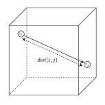
(a)

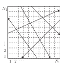
(b)

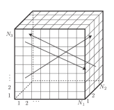
(c)

Figure 1: Multi-dimensional wireless tomography. (a) Wireless nodes are deployed on the border of the monitored region. (b) The monitored region for 2-dimensional wireless tomography. (c) The monitored region for 3-dimensional wireless tomography.

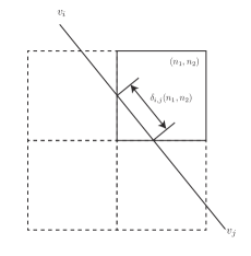
Figure 2: An example of overlap distance $\delta_{i,j}(n_{1},n_{2},\ldots,n_{D})$ on wireless link $\mathit{path}(i,j)$ between wireless nodes $v_{i}\in\cal{V}$ and $v_{j}\in\cal{V}$ for $D=2$.

IV Wireless Tomography with Compressed Sensing

We assume that $X_{n_{1},\ldots,n_{D}}$ has a high spatial correlation, which enables us to estimate $X_{n_{1},\ldots,n_{D}}$ by means of compressed sensing. In the following subsections, we first describe the wireless tomography scheme based on the vector recovery, which has been studied in [11, 14], and then, we explain the wireless tomography scheme based on the tensor recovery.

IV-A Vector Recovery-Based Wireless Tomography

We define a loss field vector $\bm{x}$ as $\bm{x}={\rm vec}(\bm{X})\in{\cal R}^{N_{1}N_{2}N_{3}N_{4}\times 1}$, and reformulate (20) as $\bm{y}=\bm{Ax}+\bm{w}$, where $\bm{A}\in{\cal R}^{M\times N_{1}N_{2}N_{3}N_{4}}$ denotes a sensing matrix. Let ${\cal F}$ denote a linear map that transforms $\bm{X}$ to its frequency domain representation such as the $D$-dimensional discrete Fourier transform (DFT) and the $D$-dimensional discrete cosine transform (DCT). In addition, let $\bm{S}={\cal F}(\bm{X})\in{\cal C}^{N_{1}\times N_{2}\times N_{3}\times N_{4}}$ and $\bm{s}=\mathrm{vec}(\bm{S})$ denote the frequency domain representation of $\bm{X}$ and its vectorization, respectively. The matrix that transforms $\bm{s}$ to $\bm{x}$ is denoted by $\bm{\Phi}\in{\cal C}^{N_{1}\cdots N_{D}\times N_{1}\cdots N_{D}}$, that is, $\bm{x}=\bm{\Phi s}$, so we have

$$\bm{y}=\bm{A\Phi s}+\bm{w}.$$

Then, let $\bm{F}_{N}=\{F_{k,n}\mid 1\leq k,n\leq N\}$ ($N\geq 1$) denote an $N\times N$ unitary matrix such as the one-dimensional DFT matrix and the one-dimensional DCT matrix. In the case of DCT, $F_{k,n}$ is given by

$$F_{n,k}=\left\{\begin{array}[]{cl}\displaystyle\frac{1}{\sqrt{N}},&k=1,1\leq n\leq N,\\ \displaystyle\sqrt{\frac{2}{N}}\cos\frac{\pi(2n+1)k}{2N},&2\leq k\leq N,1\leq n\leq N.\end{array}\right.$$

By using $\bm{F}_{N}$, $\bm{\Phi}$ can be written as

$$\bm{\Phi}=\bm{F}_{N_{1}}^{\top}\otimes\bm{F}_{N_{2}}^{\top}\otimes\bm{F}_{N_{3}}^{\top}\otimes\bm{F}_{N_{4}}^{\top},$$

where $\otimes$ represent the Kronecker product, and if $\bm{B}=\{b_{i,j}\}$ and $\bm{C}=\{c_{k,l}\}$ are $L_{1}\times L_{2}$ and $L_{3}\times L_{4}$ matrices, respectively, $\bm{B}\otimes\bm{C}$ is defined as

$$\bm{B}\otimes\bm{C}=\left(\begin{array}[]{cccc}b_{1,1}\bm{C}&b_{1,2}\bm{C}&\cdots&b_{1,L_{2}}\bm{C}\\ b_{2,1}\bm{C}&b_{2,2}\bm{C}&\cdots&b_{2,L_{2}}\bm{C}\\ \vdots&\vdots&\ddots&\vdots\\ b_{L_{1},1}\bm{C}&b_{L_{1},2}\bm{C}&\cdots&b_{L_{1},L_{2}}\bm{C}\\ \end{array}\right).$$

Consequently, we can obtain an estimate $\hat{\bm{s}}$ of the frequency domain representation $\bm{s}$ by the sparse vector recovery, as explained in section II-A, and then have the estimate $\hat{\bm{x}}$ of loss field vector $\bm{x}$ by $\hat{\bm{x}}=\bm{\Phi}\hat{\bm{s}}$.

IV-B Tensor Recovery-Based Wireless Tomography

The wireless tomography scheme based on the tensor recovery estimates the loss field tensor $\bm{X}$ from the measurement vector $\bm{y}$ by means of the tensor recovery explained in section II-C. Because each element of measurement vector $\bm{y}$ includes a noise in a practical situation, we estimate $\bm{X}$ by means of (4). Namely, from (19) and (20), we can rewrite (4) as

$$\hat{\bm{X}} = \mathop{\arg\min}_{\bm{X}}{\left(\frac{\mu}{2}\|\bm{y}-{\cal A}(\bm{X})\|_{2}^{2}+\sum_{i=1}^{D}\|\bm{X}_{(i)}\|_{*}\right)}$$

$$= \mathop{\arg\min}_{\bm{X}}\left(\frac{\mu}{2}\sum_{n_{4}=1}^{N_{4}}\|\bm{y}^{(n_{4})}-{\cal A}^{(n_{4})}(\bm{X}^{(n_{4})})\|_{2}^{2}\right.$$

$$\left.+\sum_{i=1}^{D}\|\bm{X}_{(i)}\|_{\ast}\right).$$

It is worth mentioning that the matrix recovery-based wireless tomography corresponds to the tensor recovery-based wireless tomography for $D=2$. Therefore, in the following, we use the tensor recovery-based wireless tomography for $D=2$ and the matrix recovery-based wireless tomography exchangeably.

V Performance Evaluation

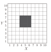
(a) $D=2$.

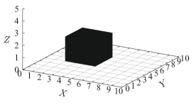
(b) $D=3$.

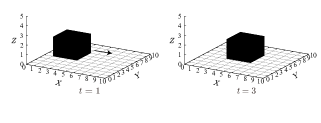
(c) $D=4$.

Figure 3: Monitored regions for simulation experiments.

V-A Simulation Setup

In this section, we demonstrate the performance of the tensor recovery scheme by comparing it with that of the vector recovery scheme for $D=2,3,4$. Figs. 3a, 3b, and 3c show the monitored regions for $D=2$, $D=3$, and $D=4$, respectively. In the case of $D=2$, we set $N_{1}=N_{2}=10$ and place a $3\times 3$ square-shaped obstruction in the monitored region, which is represented by dark pixels in Fig. 3a. The elements of $\bm{X}\in\mathcal{R}^{N_{1}\times N_{2}}$ are set to $10$ within the dark pixels and $0$ within the other pixels. 40 wireless nodes are placed on the border of the monitored region as shown in Fig. 4a. Next, in the case of $D=3$, we set $N_{1}=N_{2}=10,\ N_{3}=5$ and place a $3\times 3\times 2$ obstruction, which is represented by dark voxels in Fig. 3b. The elements of $\bm{X}\in\mathcal{R}^{N_{1}\times N_{2}\times N_{3}}$ are set to $10$ within the dark voxels and $0$ within the other pixels. 200 wireless nodes are placed on the sides of the monitored region as shown in Fig. 4b. Finally, in the case of $D=4$, we set $N_{1}=N_{2}=10$, $N_{3}=5$, and $N_{4}=3$, where the monitored region is the same environment as the case of $D=3$ and the obstruction is moving as shown in Fig. 3c.

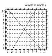
(a) $D=2$.

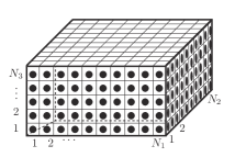
(b) $D=3,4$.

Figure 4: Node placement in simulation experiments.

In each simulation experiment, $M$ pairs of wireless nodes are randomly chosen to establish $M$ wireless links, and in each pair, a randomly chosen node is set to a transmitter and the other is set to a receiver. We assume that each measurement is contaminated with a Gaussian noise with zero mean and variance $\eta^{2}$.

In the vector recovery scheme, we use the DCT to transform the loss field tensor $\bm{X}$ to its frequency representation, and estimate the loss field tensor by solving the optimization problem (1) with FISTA [2, 19]. The regularization parameter $\lambda$ in (1) is set to $1.0$. On the other hand, in the tensor recovery scheme, we estimate the loss field tensor $\bm{X}$ by solving the optimization problem (3) [17] for $D=2$ and the optimization problem (4) [7] for $D=3,4$. The regularization parameter $\mu$ is set to $1.0$. Note that in this paper, we do not consider the optimization of the regularization parameters $\lambda$ and $\mu$, which is beyond the scope of the paper.

We evaluate the performance of the vector and tensor recovery schemes in terms of the normalized reconstruction error $\epsilon$ between the true loss field tensors and the corresponding estimated loss field tensors. In more detail, for given $M$ and $\eta$, we conduct $N_{\rm run}$ independent simulation experiments to calculate $\epsilon$, which is defined as

$$\epsilon=\frac{1}{N_{\rm run}}\sum_{i=1}^{N_{\rm run}}\frac{\|\hat{\bm{X}_{[i]}}-\bm{X}\|_{\rm F}}{\|\bm{X}\|_{\rm F}}.$$ (21)

In (21), $\hat{\bm{X}}_{[i]}$ ($i=1,2,\ldots,N_{\rm run}$) denote the estimated loss field tensor obtained by the $i$-th simulation experiment and $\|\cdot\|_{\rm F}$ represents the Frobenius norm. Here, for $\bm{{\rm Z}}=\{Z_{n_{1},n_{2},\ldots,n_{D}}\mid n_{i}=1,2,\ldots,N_{i},i=1,2,\ldots,D\}\in\mathcal{R}^{N_{1}\times N_{2}\times\cdots N_{D}}$, its Frobenius norm is defined as

$$\|\bm{{\rm Z}}\|_{\rm F}=\left(\sum_{n_{1}=1}^{N_{1}}\sum_{n_{2}=1}^{N_{2}}\cdots\sum_{n_{D}=1}^{N_{D}}Z_{n_{1},n_{2},\ldots,n_{D}}^{2}\right)^{\frac{1}{2}}.$$

V-B Simulation Results

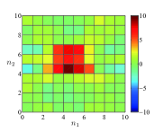
(a) Vector recovery.

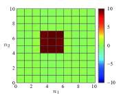
(b) Matrix recovery.

Figure 5: Examples of the estimated loss field tensor ($D=2$, $M=60$, $\eta=0$).

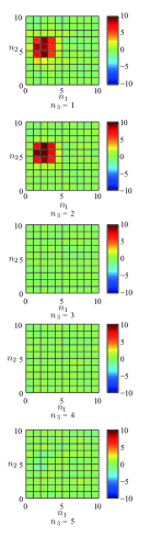
(a) Vector recovery

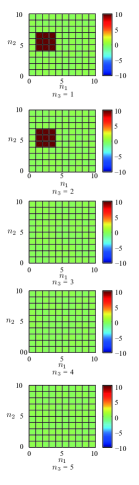
(b) Tensor recovery

Figure 6: Examples of the estimated loss field tensor using the vector and tensor recovery-based wireless tomography  ($D=3$, $M=300$, $\eta=0$).

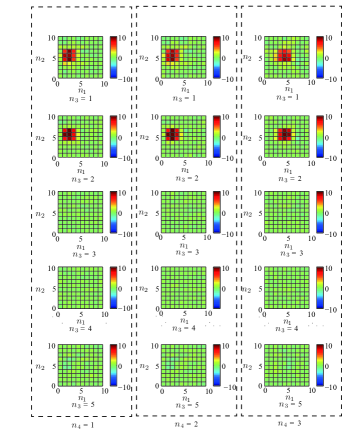
(a) Vector recovery.

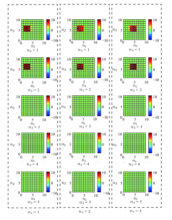
(b) Tensor recovery.

Figure 7: Examples of the estimated loss field tensor ($D=4$, $M=900$, $M_{n_{4}}=300$ $(n_{4}=1,2,3)$, $\eta=0$).

Figs. 5, 6, and 7 show examples of the estimated loss field tensors for $D=2$, $3$, and $4$, respectively. For each figure, we show the loss field tensors estimated by the vector and tensor recovery schemes in the noiseless environment (i.e., $\eta=0$). Here, the number ($M$) of measurements is set to $60$ for the case of $D=2$, and $M$ is set to $300$ for the case of $D=3$. For the case of $D=4$, furthermore, $M$ is set to $900$, and the number $M_{n_{4}}$ $(n_{4}=1,2,3)$ of measurements at time $n_{4}$ is set to $300$. From these figures, we observe that the tensor recovery scheme (i.e., Figs. 5b, 6b, and 7b) can estimate the loss field tensor more accurately than the vector recovery scheme (i.e., Figs. 5a, 6a, and 7a).

For fair comparison of the results obtained in different dimensions, we define the normalized number $\gamma$ of measurements as

$$\gamma=\frac{M}{N_{1}N_{2}N_{3}N_{4}},$$

where $N_{3}=N_{4}=1$ for $D=2$ and $N_{4}=1$ for $D=3$. Figs. 8, 9, and 10 show the reconstruction error $\epsilon$ vs. $\gamma$ in the noiseless environment (i.e., $\eta=0$) for $D=2$, $3$, and $4$, respectively. In these figures, “DCT”, “Matrix”, and “Tensor” represent the performances of the vector, matrix and tensor recovery schemes, respectively, where we set the number $N_{\rm run}$ of simulation experiments for each parameter to $50$. From these figures, we observe that the tensor recovery scheme can achieve lower reconstruction errors than the vector recovery scheme.

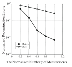
Figure 8: The normalized reconstruction error $\epsilon$ vs. the number $M$ of measurements ($D=2$, $\eta=0$).

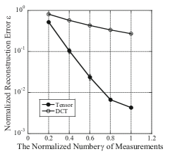
Figure 9: The normalized reconstruction error vs. the number $M$ of measurements ($D=3$, $\eta=0$).

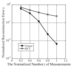
Figure 10: The normalized reconstruction error vs. the number $M$ of measurements ($M=4$, $\eta=0$).

Figs. 11, 12, and 13 show the normalized reconstruction error $\epsilon$ vs. the standard deviation $\eta$ of noise for $D=2$, $3$, and $4$, respectively, where we set $M=60$ for $D=2$, $M=300$ for $D=3$, and $M=900$ and $M_{n_{4}}=300$ ($n_{4}=1,2,3$) for $D=4$. For the cases of $D=2$ and $3$, we observe that the tensor recovery scheme has lower reconstruction errors even in the noisy environments. For the case of $D=4$, however, we observe that the tensor recovery scheme achieves a better performance than the vector recovery scheme only for smaller $\eta$. These figures indicate that the tensor recovery scheme is vulnerable to the measurement noise. Therefore, in order to ensure the performance gain by the tensor recovery scheme, measurement techniques with smaller observation noise are required, where we leave it as a future work.

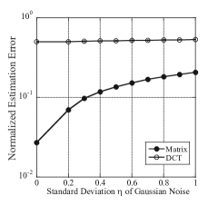
Figure 11: The normalized reconstruction error $\epsilon$ vs. standard deviation $\eta$ of noise ($D=2$, $M=60$).

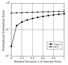
Figure 12: The normalized reconstruction error vs. standard deviation $\eta$ of noise ($D=3$, $M=300$).

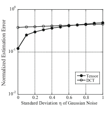
Figure 13: The normalized reconstruction error vs.  standard deviation $\eta$ of noise ($D=4$, $M=900$).

V-C Discussion: Vector Recovery vs. Tensor Recovery

In this subsection, we discuss the reason why the tensor recovery scheme can achieve more accurate estimation of loss field tensors than the vector recovery scheme, as shown in the previous subsection. In order to simplify the discussion, we focus on the case of $D=2$.

In the vector recovery scheme, by using the frequency domain representation $\bm{S}$, the loss field tensor $\bm{X}$ can be written as [10]

$$\bm{X}=\bm{F}_{N_{1}}^{\rm\top}\bm{S}\bm{F}_{N_{2}}.$$

When $\bm{X}$ has a high spatial correlation, most of the energy in $\bm{X}$ is concentrated in a few low-frequency elements of $\bm{S}$, that is, $\bm{S}$ is an approximately sparse matrix. Therefore, when applying the vector recovery to the measurement vector $\bm{y}$, we obtain a sparsified matrix $\hat{\bm{S}}$ by replacing the elements with a smaller absolute value in $\bm{S}$ with zeros. We thus obtain the estimated loss field tensor $\hat{\bm{X}}^{\rm(V)}$ as

$$\hat{\bm{X}}^{\rm(V)}=\bm{F}_{N_{1}}^{\rm\top}\hat{\bm{S}}\bm{F}_{N_{2}}.$$

The reconstruction error $\kappa_{\rm(V)}$ of $\hat{\bm{X}}^{\rm(V)}$ is then given by

$$\kappa_{\rm(V)}=\|\hat{\bm{X}}^{\rm(V)}-\bm{X}\|_{\rm F}.$$

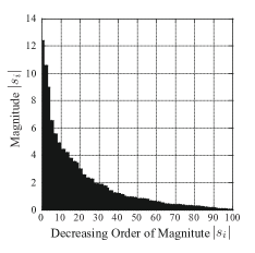
(a) Frequency representation of a loss field tensor

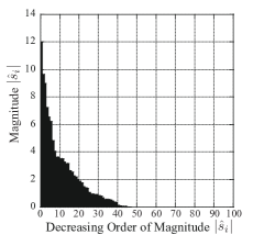
(b) Frequency representation of a loss field Tensor estimated by the vector recovery scheme.

Figure 14: An example of ordered spectrum of a loss field tensor.

Figs. 14a and 14b show $|s_{i}|$ and $|\hat{s}_{i}|$ $(i=1,2,\ldots,N_{1}N_{2})$ sorted in the decreasing order, where $\bm{s}=\mathrm{vec}(\bm{S})=(s_{1}~{}s_{2}~{}\cdots~{}s_{N_{1}N_{2}})^{\top}$ and $\hat{\bm{s}}=\mathrm{vec}({\hat{\bm{S}}})=(\hat{s}_{1}~{}\hat{s}_{2}~{}\cdots~{}\hat{s}_{N_{1}N_{2}})^{\top}$ are defined as the vectorization of $\bm{S}$ and $\hat{\bm{S}}$, respectively. We observe that $\hat{\bm{s}}$ is obtained by replacing the smaller elements of $\bm{s}$ with zeros.

On the other hand, in the tensor recovery scheme, the reconstruction error can be explained with SVD. Namely, let us define $\sigma_{i}\ (i=1,2,\ldots,r)$ as singular values of $\bm{X}$, where $r=\min\{N_{1},N_{2}\}$. With matrices $\bm{U}\in{\cal R}^{N_{1}\times r}$ and $\bm{V}\in{\cal R}^{N_{2}\times r}$ whose column vectors are orthogonal, the SVD of $\bm{X}$ can be written as

$$\bm{X}=\bm{U\Sigma V}^{\top},$$

where $\bm{\Sigma}={\rm diag}(\sigma_{1},\sigma_{2},\ldots,\sigma_{r})$ denotes an $r\times r$ diagonal matrix.

Without loss of generality, we can assume that singular values $\sigma_{i}\ (i=1,2,\ldots,r)$ are arranged in the decreasing order, i.e., $\sigma_{1}\geq\sigma_{2}\geq\cdots\geq\sigma_{r}\geq 0$. Applying the tensor recovery scheme to the measurement vector $\bm{y}$, we obtain a diagonal matrix $\hat{\bm{\Sigma}}=\mathrm{diag}(\hat{\sigma}_{1},\hat{\sigma}_{2},\ldots,\hat{\sigma}_{r})$ by replacing the $r-K$ smaller diagonal elements of $\bm{\Sigma}$ with zeros, that is, $\hat{\sigma}_{i}\approx\sigma_{i}$ $(i=1,2,\ldots,K)$, $\hat{\sigma}_{K+1}=\hat{\sigma}_{K+2}=\cdots=\hat{\sigma}_{r}=0$. We thus obtain estimated loss field tensor $\hat{\bm{X}}^{(\rm M)}$ as

$$\hat{\bm{X}}^{\rm(M)}=\bm{U}\hat{\bm{\Sigma}}\bm{V}^{\top}.$$

The reconstruction error $\kappa_{\rm(M)}$ of $\hat{\bm{X}}^{(\rm M)}$ is then given by

$$\kappa_{\rm(M)}=\|\hat{\bm{X}}^{\rm(M)}-\bm{X}\|_{\rm F}.$$

Table I shows singular values of the true loss field tensor and an estimated loss field tensor. Because the rank of the loss field tensor $\bm{X}$ in Fig. 3a is $\mathrm{rank}\bm{X}=1$, $\bm{X}$ has only one non-zero singular value $\sigma_{1}$. The estimated loss field tensor $\hat{\bm{X}}$ highly approximates $\bm{X}$ by replacing $\sigma_{i}$ ($i=3,4,\ldots,N_{1}N_{2}$) with zeros.

TABLE I: Singular values of a loss field tensor and its estimated loss field tensor ($D=2$, $M=60$).

$i$	$1$	$2$	$3,4,\ldots,N_{1}N_{2}$
$\sigma_{i}$	$30.00$	$0$	$0$
$\hat{\sigma}_{i}$	$29.68$	$0.001244$	$0$

Finally, suppose that both $\hat{\bm{S}}$ and $\hat{\bm{\Sigma}}$ generally have $K$ non-zero elements. For the case of $D=2$, it is well-known that SVD provides the smallest reconstruction error, that is, $\kappa_{\rm(M)}\leq\kappa_{\rm(V)}$ [10, 6], where $\kappa_{\rm(M)}$ is given by

$$\kappa_{\rm(M)}=\sqrt{\sum_{i=K+1}^{r}\sigma_{i}^{2}}.$$

Therefore, for the case of $D=2$, the tensor recovery scheme is the best way in terms of the reconstruction error. Actually, in [6], the authors show that the SVD-based image compression obtains better reconstruction errors than the DCT-based image compression. Furthermore, in [13], HOSVD is studied and it is shown that low-rank approximation of the $D$-th tensor provides a good approximation in terms of the reconstruction error.

VI Conclusion

In this paper, we proposed a multi-dimensional wireless tomography using tensor-based compressed sensing, which enables us to estimate the locations of internal obstructions by a small number of measurement signals. While the conventional wireless tomography using the vector recovery-based compressed sensing utilizes the sparsity of the frequency representation of a given loss field tensor, the proposed wireless tomography utilizes its low-rank property. With simulation experiments, we validated the effects of the proposed wireless tomography, and showed that the tensor recovery-based wireless tomography can provide more accurate estimation of the loss field tensor, especially in a less noisy environment.

We still have some remaining issues to be resolved. For example, in order to achieve noiseless measurements, we require a signal processing technique to extract a direct link in multipath fading environments. In this paper, we assumed that many wireless nodes are deployed on the border of the monitored region, and we chose wireless links randomly by using these wireless nodes. In a situation where there are a small number of wireless nodes, however, we have to consider a wireless node selection scheme to achieve an efficient estimation of a loss field tensor. We will try these issues in the future work.

References

- [1] P. Agrawal and N. Patwari, “Correlated link shadow fading in multi-hop wireless networks,” IEEE Transactions on Wireless Communications, vol. 8, no. 8, pp. 4024–4036, Aug. 2009.
- [2] A. Beck and M. Teboulle, “A fast iterative shrinkage-thresholding algorithm for linear inverse problems,” SIAM Journal on Imaging Sciences, vol. 2, no. 1, pp. 183–202, 2009.
- [3] C. F. Caiafa and A. Cichocki, “Computing sparse representations of multidimensional signals using Kronecker bases,” Neural Computation, vol. 25, no. 1, pp. 186–220, Jan. 2013.
- [4] E. J. Candès and M. B. Wakin, “An introduction to compressive sampling,” IEEE Signal Processing Magazine, vol. 25, no. 2, pp. 21–30, Mar. 2008.
- [5] J. Chen and Y. Saad, “On the tensor SVD and the optimal low rank orthogonal approximation of tensors,” SIAM Journal on Matrix Analysis and Applications, vol. 30, no. 4, pp. 1709–1734, 2009.
- [6] A. Dapena and S. Ahalt, “A hybrid DCT-SVD image-coding algorithm,” IEEE Transactions on Circuits and Systems for Video Technology, vol. 12, no. 2, pp. 114–121, Feb. 2002.
- [7] S. Gandy, B. Recht, and I. Yamada, “Tensor completion and low-n-rank tensor recovery via convex optimization,” Inverse Problems, vol. 27, no. 2, Feb. 2011.
- [8] H. Hashemi, “The indoor radio propagation channel,” Proceedings of the IEEE, vol. 81, no. 7, pp. 943–968, Jul. 1993.
- [9] K. Hayashi, M. Nagahara, and T. Tanaka, “A user’s guide to compressed sensing for communications systems,” IEICE Transactions on Communications, vol. E96-B, no. 3, pp. 685–712, Mar. 2013.
- [10] A. K. Jain, Fundamentals of Digital Image Processing, Prentice Hall, 1989.
- [11] M. A. Kanso and M. G. Rabbat, “Compressed RF tomography for wireless sensor networks: centralized and decentralized approaches,” in Proc. the 5th IEEE International Conference on Distributed Computing in Sensor Systems, pp. 173–186, Jun. 2009.
- [12] T. G. Kolda and B. W. Bader, “Tensor decompositions and applications,” SIAM Review, vol. 51, no. 3, pp. 455–500, Aug. 2009.
- [13] L. D. Lathauwer, B. D. Moor, and J. Vandewalle, “A multilinear singular value decomposition,” SIAM Journal on Matrix Analysis and Applications, vol. 21, no. 4, pp. 1253–1278, 2000.
- [14] Y. Mostofi, “Compressive cooperative sensing and mapping in mobile networks,” IEEE Transactions on Mobile Computing, vol. 10, no. 12, pp. 1769–1784, Dec. 2011.
- [15] N. Patwari and P. Agrawal, “Effects of correlated shadowing: connectivity, localization, and RF tomography,” in Proc. International Conference on Information Processing in Sensor Networks, pp. 82–93, Apr. 2008.
- [16] B. Recht, M. Fazel, and P. A. Parrilo, “Guaranteed minimum-rank solutions of linear matrix equations via nuclear norm minimization,” SIAM Review, vol. 52, no. 3, pp. 471–501, 2010.
- [17] K. C. Toh and S. Yun, “An accelerated proximal gradient algorithm for nuclear norm regularized linear least squares problems,” Pacific Journal of Optimization, vol. 6, no. 3, pp. 615–640, Sep. 2010.
- [18] J. Wilson and N. Patwari, “Radio tomographic imaging with wireless networks,” IEEE Transactions on Mobile Computing, vol. 9, no. 5, pp. 621–632, May 2010.
- [19] M. Zibulevsky and M. Elad, “L1-L2 optimization in signal and image processing,” IEEE Signal Processing Magazine, vol. 27, no. 3, pp. 76–88, May 2010.