Blind Interference Alignment in General Heterogeneous Networks

Abstract

Heterogeneous networks have a key role in the design of future mobile communication networks, since the employment of small cells around a macrocell enhances the network’s efficiency and decreases complexity and power demand. Moreover, research on Blind Interference Alignment (BIA) has shown that optimal Degrees of Freedom (DoF) can be achieved in certain network architectures, with no requirement of Channel State Information (CSI) at the transmitters. Our contribution is a generalised model of BIA in a heterogeneous network with one macrocell with $K$ users and $K$ femtocells each with one user, by using Kronecker (Tensor) Product representation. We introduce a solution on how to vary beamforming vectors under power constraints to maximize the sum rate of the network and how optimal DoF can be achieved over $K+1$ time slots.

I Introduction

Next-generation mobile and cellular networks will require higher capacity and reliabilty, as well as power-efficiency. Interference Alignment (IA), first introduced by Maddah-Ali, Motahari and Khandani in [1] and Cadambe and Jafar in [2], made a very promising step in this direction by proving that it is possible that the $K$-user interference channel, under the assumption of global perfect CSI, can have $K/2$ DoF, i.e. “everyone gets half the cake”. The novelty of the IA scheme, as described in [1]-[3], lies in the fact that it attempts to align, rather than cancel or reduce, interference along dimensions different from the dimensions of the actual signal.

Initially, the main drawbacks of IA were the requirement of global perfect CSI at the transmitter (CSIT), which resulted in feedback overhead, and its complexity, as only for the $K=3$ case, as presented in [4], a closed-form solution could be easily described. In general, in the absence of perfect or partial CSIT, the DoF of a network collapse, i.e transmissions are no longer reliable. However, for certain networks, the scheme of Blind IA (BIA), originally presented by Wang, Gou and Jafar in [5] and Jafar in [6], can achieve full DoF, even when no CSIT is available. BIA can be successfully achieved by a) knowing distinct coherence patterns associated with different receivers, or b) employing distinct antenna switching patterns at receivers equipped with reconfigurable antennas. Furthermore, as suggested by Jafar in [7], BIA can achieve even higher than $K/2$ DoF in certain cellular environments simply by seeing frequency reuse as a simple form of IA. Moreover, [7] introduced the feasibility of BIA in heterogenous networks due to interference diversity, i.e. the observation that every receiver experiences a different set of interferers, and depending on the actions of its interferers, the interference-free signal subspace fluctuates differently from the rest of the receivers. Finally, [8] and [9] introduced an equal-power allocation BIA scheme that reduces noise enhancement by constant power transmission.

In this paper, based on [5]-[7], we propose a generalised model of BIA in a heterogeneous network, where there is one macrocell with $K$ users and $K$ femtocells with one user each (see Figure 1). Our contribution is the generalisation of the construction given by Jafar, [7, Section 6] in the case $K=2$, introducing the application of BIA to heterogeneous networks. Moreover, this paper introduces a new description of the BIA model using a Kronecker Product representation. Based on our findings, the DoF that can be achieved in both tiers of the network are presented. Finally, we discuss how to vary parameters of the model to maximize sum rate, extending the ideas of [8]-[9], and demonstrating optimality in the sum rate sense.

The rest of the paper is organized as follows. Section II presents the general description of the BIA model, including the determination of the beamforming matrices, and the whole decoding process. Section III presents the DoF that can be achieved in the macrocell and the $K$ femtocells. Section IV presents the achievable sum rate formula for the heterogenous network. Finally, Section V gives an overview of our results, illustrated with the aid of simulations/graphs.

II System Model

We generalise Jafar’s model [7, Section 6], under the same channel assumptions. Consider the Broadcast Channel (BC) of a heterogeneous network, as shown in Figure 1, with 1 macrocell and $K$ femtocells. At the $N\times N$ MIMO BC of the macrocell, there is one transmitter $T_{xA}$ with $N$ antennas, and $K$ users equipped with $N$ antennas each. Transmitter $T_{xA}$ has $N$ messages to send to every user, and furthermore, when it transmits to user $a_{k}$, where $k\in\left\{1,2,...,K\right\}$, it causes interference to all the other $K-1$ users in the macrocell. At the $M_{r}\times N$ MIMO BC of each femtocell, there is one transmitter $T_{xk}$ with $N$ antennas, and one user $f_{k}$ equipped with $M_{r}$ antennas, with $M{}_{r}=N-1$. Transmitter $T_{xk}$ has $\mathcal{M}=(T-1)M_{r}+1$ messages to send to the femtocell user $f_{k}$, and when it transmits to $f_{k}$, it causes interference to the macrocell user $a_{k}$. The operation is performed over $T=K+1$ channel uses (i.e. time slots), which constitute a supersymbol. The channel is assumed to remain constant over the supersymbol.

The BIA scheme works by using different antenna switching patterns for each of the $K$ femtocells. These switching patterns are encoded in the indicator vectors as described later in this section. For the successful application of the BIA scheme, the following assumptions, as in [7], are made:

• Users in the femtocells do not receive any interference from transmissions in the macrocell

• No CSIT is required, only knowledge of the connectivity of the network is available at the transmitters

II-A Beamforming Matrices

II-A1 Macrocell

The $((NT)\times 1$) signal at receiver $a_{k}$, for the supersymbol, is given by:

$$\mathbf{y}^{[a_{k}]}=\mathbf{H}^{[a_{k}]}\mathbf{X}{}_{A}+\mathbf{H}^{[f_{k}a_{k}]}\mathbf{X}_{f_{k}}+\mathbf{Z}^{[a_{k}]}$$ (1)

Channel transfer matrices are statistically independent due to users’ different locations, and each one of their entries follows an i.i.d. Gaussian distribution $\mathcal{CN}(0,1)$. $\mathbf{H}^{[a_{k}]}\in\mathcal{\mathcal{C}}^{NT\times NT}$ is the channel transfer matrix from $T_{xA}$ to $a_{k}$, and is given by $\mathbf{H}^{[a_{k}]}=\mathbf{I}_{T}\otimes\mathbf{h}^{[a_{k}]}$ (here and throughout $\otimes$ represents the Kronecker (Tensor) product), as the channel is non-varying, where $\mathbf{h}^{[a_{k}]}\in\mathcal{\mathcal{C}}^{N\times N}$ is the channel for one time slot. $\mathbf{H}^{[f_{k}a_{k}]}\in\mathcal{C}^{NT\times NT}$ is the inter-cell interference channel transfer matrix from $T_{x_{k}}$ to $a_{k}$, and is given by $\mathbf{H}^{[f_{k}a_{k}]}=\mathbf{I}_{T}\otimes\mathbf{h}^{[f_{k}a_{k}]}$, where $\mathbf{h}^{[f_{k}a_{k}]}\in\mathcal{\mathcal{C}}^{N\times N}$ is the channel for one time slot. Finally, $\mathbf{Z}^{[a_{k}]}\sim\mathit{\mathcal{CN}}(0,\sigma_{n}^{2}\mathbf{I}_{NT})$ denotes the independent Additive White Gaussian Noise (AWGN) vector.

The ($N\times 1$) data stream vector of each user $a_{k}$ is given by $\mathbf{U}^{[a_{k}]}$. The choice of the ($(NT)\times N$) beamforming matrices $\mathbf{V}^{[a_{k}]}$ carrying messages to users in the macrocell is not unique and should lie in a space that is orthogonal to the channels of the other $K-1$ macrocell users.

$$\mathbf{V}^{[a_{k}]}=\frac{a}{\sqrt{N}}(\mathbf{v}^{[a_{k}]}\otimes\mathbf{I}_{N}),$$ (2)

where $a\in\mathrm{\mathfrak{\boldsymbol{\mathfrak{\mathcal{\mathbb{R}}}}}}$ is a constant determined by power considerations (see (4)), and ($T\times 1$) $\mathbf{v}^{[a_{k}]}$ should be a unit vector with entries equal to $c$, $\sqrt{1-c^{2}}$ (for $c\in\mathrm{\mathfrak{\boldsymbol{\mathfrak{\mathcal{\mathbb{R}}}}}}$ and $c\neq 0,\pm 1$) or $0$, with a different combination for every $a_{k}$. For every macrocell user, there will be one time slot in which only they will be receiving messages. Also, there will be another time slot (time slot 2 in Figure 2) over which $T_{xA}$ will transmit to all users. The $((NT)\times 1)$ vector $\mathbf{X}{}_{A}$ transmitted by $T_{xA}$, is given by:

$$\mathbf{X}{}_{A}=\sum_{i=1}^{K}\mathbf{V}^{[a_{i}]}\mathbf{U}^{[a_{i}]}$$ (3)

The total transmit power is given by the power constraint:

$$P_{\mathrm{macrocell}}=\mathbb{E}[\mathrm{tr}(\mathbf{X}_{A}\mathbf{X}_{A}^{T})]=KNa^{2}$$ (4)

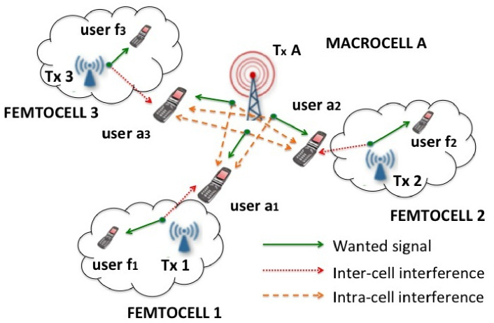
Figure 1: BIA in a heterogeneous network: $K=3$ users in the macrocell and $K=3$ femtocells with 1 user each

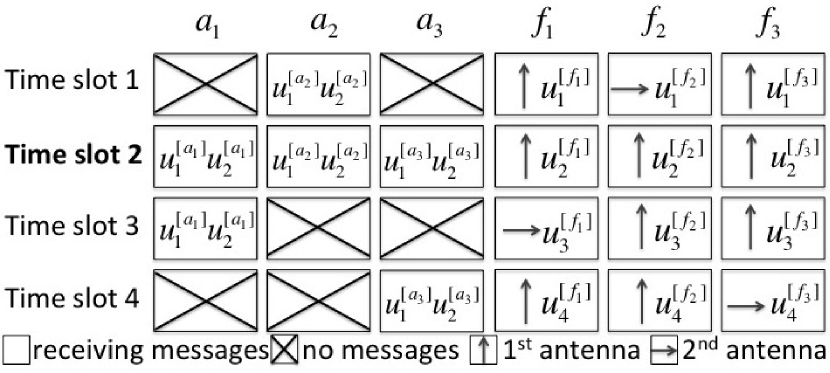
Figure 2: Beamforming in macrocell and femtocells

Example 1.

The same model will be used as an example in this paper: For $K=3$ users in the macrocell with $N=2$ transmit/receive antennas and messages for each user, $M_{r}=1$ receive and $N=2$ transmit antennas and $\mathcal{M}=4$ messages sent in each one of the $K=3$ femtocells, and $T=4$ time slots, the beamforming matrices, as shown in Figure 2, are given by:

$\mathbf{V}^{[a_{1}]}=\frac{a}{\sqrt{N}}(\mathbf{v}^{[a_{1}]}\otimes\mathbf{I}_{2})=\frac{a}{\sqrt{2}}\bigl{[}\begin{array}[]{cccc}0&c&\sqrt{1-c^{2}}&0\end{array}\bigr{]}^{T}\otimes\mathbf{I}_{2}$

$\mathbf{V}^{[a_{2}]}=\frac{a}{\sqrt{N}}(\mathbf{v}^{[a_{2}]}\otimes\mathbf{I}_{2})=\frac{a}{\sqrt{2}}\bigl{[}\begin{array}[]{cccc}\sqrt{1-c^{2}}&c&0&0\end{array}\bigr{]}^{T}\otimes\mathbf{I}_{2}$

$\mathbf{V}^{[a_{3}]}=\frac{a}{\sqrt{N}}(\mathbf{v}^{[a_{3}]}\otimes\mathbf{I}_{2})=\frac{a}{\sqrt{2}}\bigl{[}\begin{array}[]{cccc}0&c&0&\sqrt{1-c^{2}}\end{array}\bigr{]}^{T}\otimes\mathbf{I}_{2}$

II-A2 Femtocells

At each femtocell, the ($(M_{r}T)\times 1$) signal at receiver $f_{k}$, for the supersymbol, is given by:

$$\mathbf{y}^{[f_{k}]}=\mathbf{H}^{[f_{k}]}\mathbf{X}{}_{f_{k}}+\mathbf{Z}^{[f_{k}]},$$ (5)

where $\mathbf{H}^{[f_{k}]}\in\mathcal{C}^{M_{r}T\times NT}$ is the channel transfer matrix from $T_{xf}$ to$f_{k}$, and is given by ${\color[rgb]{0,0,0}\mathbf{H}^{[f_{k}]}=\mathbf{I}_{T}\otimes\mathbf{h}^{[f_{k}]}}$ where $\mathbf{h}^{[f_{k}]}\in\mathcal{\mathcal{C}}^{M_{r}\times N}$ is the channel for one time slot, and $\mathbf{Z}^{[f_{k}]}\sim(0,\sigma_{n}^{2}\mathbf{I}_{M_{r}T})$ denotes the Additive White Gaussian Noise (AWGN) vector.

In each femtocell, the ($\mathcal{M}\times 1$) data stream vector of each user $f_{k}$ is given by $\mathbf{U}^{[f_{k}]}$. The $((NT)\times\mathcal{M})$ beamforming matrix $\mathbf{V}^{[f_{k}]}$ is given by:

$$\mathbf{V}^{[f_{k}]}=\frac{b}{\sqrt{N}}\left(\sum_{i=1}^{T}\mathbf{\mathbf{\gamma}}_{i}^{[f_{k}]^{T}}\otimes\mathbf{r}_{i}\mathbf{q}_{i}\right)$$ (6)

where $b\in\mathrm{\mathfrak{\boldsymbol{\mathfrak{\mathcal{\mathbb{R}}}}}}$ is a constant determined by power considerations (see (8)), and $\mathbf{v}_{1}^{[f_{k}]}=\sum_{i=1}^{T-1}\mathbf{\gamma}_{i}^{[f_{k}]}$ and $\mathbf{v}_{2}^{[f_{k}]}=\mathbf{\gamma}_{T}^{[f_{k}]}$ are ($1\times T$) unit vectors with entries equal to 1 and 0, with $\mathbf{v}_{2}^{[f_{k}]}$ having only its $t$th entry ($t$ denoting the time slot that $a_{k}$ receives no interference) equal to 1, such that $\sum_{j=1}^{2}\mathbf{v}_{j}^{[f_{k}]}=\begin{bmatrix}1&1&...&1\end{bmatrix}$. Also, for $i=1,...,T-1$, we set $\mathbf{r}_{i}$ equal to the first $M_{r}$ columns of $\mathbf{I}_{N}$ with $\mathbf{e}_{1}$ equal to the sum of the columns of $\mathbf{r}_{i}$, and $\mathbf{e}_{2}=\mathbf{r}_{T}$ equal to the last column of $\mathbf{I}_{N}$. Furthermore, for $i=1,...,T-1$, $\mathbf{q}_{i}$ is equal to the submatrix of $\mathbf{I}_{\mathcal{M}}$ consisting of rows $(M_{r}(i-1)+1,M_{r}i),$ and $\mathbf{q}_{T}$ is equal to the submatrix of $\mathbf{I}_{\mathcal{M}}$ consisting of row $\mathcal{M}$. The $t$th component of $\mathbf{\gamma}_{i}^{[f_{k}]}$ being 1 means that in the $k$th femtocell, the antennas determined by $\mathbf{r}_{i}$ are in use at time $t$, and the messages determined by $\mathbf{q}_{i}$ are transmitted. Finally, the ($(NT)\times 1$) vector, transmitted by $T_{xK}$ is given by:

$$\mathbf{X}{}_{f_{k}}=\mathbf{V}^{[f_{k}]}\mathbf{U}^{[f_{k}]}$$ (7)

The total transmit power is given by the power constraint:

$$P_{\mathrm{femtocell}}=\mathbb{E}[\mathrm{tr}(\mathbf{X}_{f_{k}}\mathbf{X}_{f_{k}}^{T})]=\mathcal{M}^{2}\frac{b^{2}}{N}$$ (8)

Example 2.

For our example-model, the beamforming matrix for user $f_{1}$, as depicted in Figure 2, is given by:

$\mathbf{V}^{[f_{1}]}=\frac{b}{\sqrt{2}}\left(\sum_{i=1}^{4}\mathbf{\mathbf{\gamma}}_{i}^{[f_{1}]^{T}}\otimes\mathbf{r}_{i}\mathbf{q}_{i}\right)$

with $\sum_{i=1}^{3}\mathbf{\gamma}_{i}^{[f_{1}]}=\mathbf{v}_{1}^{[f_{1}]}=[\begin{array}[]{cccc}{\normalcolor 1}&1&{\normalcolor 0}&1\end{array}]$ , $\mathbf{\gamma}_{4}^{[f_{1}]}=\mathbf{v}_{2}^{[f_{1}]}=[\begin{array}[]{cccc}{\color[rgb]{0,0,0}0}&{\color[rgb]{0,0,0}0}&1&{\color[rgb]{0,0,0}0}\end{array}]$

for $i=1,2,3:$ $\mathbf{r}_{i}=\begin{bmatrix}1&0\end{bmatrix}^{T}$with $\mathbf{e}_{1}=\begin{bmatrix}1&0\end{bmatrix}^{T}$, $\mathbf{r}_{4}=\mathbf{e}_{2}=\begin{bmatrix}0&1\end{bmatrix}^{T}$,

$\mathbf{q}_{i}$ the ith unit basis vector

II-B Projection & Effective Channel Matrix

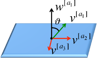
Figure 3: Schematic plot of beamforming vectors: $\mathbf{w}_{s}^{[a_{1}]}$ is orthogonal to $\mathbf{v}^{[a_{2}]}$ ,$\mathbf{v}^{[a_{3}]}$ .

II-B1 Macrocell

In the macrocell, in order remove inter- and intra-cell interference, the received signal should be projected to a subspace orthogonal to the subspace that interference lies in. The rows of the ($N\times NT$) projection matrix $\mathbf{P}^{[a_{k}]}$ form an orthonormal basis of this subspace:

$$\mathbf{P}^{[a_{k}]}={\displaystyle\sum_{s=1}^{2}}\left(\mathbf{w}_{s}^{[a_{k}]}\otimes\mathbf{D}_{s}^{[a_{k}]}\mathbf{\widetilde{h}}^{[f_{k}a_{k}]}\right),$$ (9)

where

1. for all s, the ($1\times T$) $\mathbf{w}_{s}^{[a_{k}]}$ is a unit vector orthogonal to $\mathbf{v}^{[a_{i}]}$ for $i\neq k$, as shown in Figure 3,

2. $\mathbf{w}_{s}^{[a_{k}]}$ has coefficients equal to zero on the non-zero values of $\mathbf{\mathbf{\gamma}}_{i}^{[f_{k}]^{T}}$ for $s=1$ and $i=T$, and for $s=2$ and $i=1...T-1$,

3. $\mathbf{D}_{1}^{[a_{k}]}=\mathrm{diag}(\mathbf{e}_{2})$ and $\mathbf{D}_{2}^{[a_{k}]}=\mathrm{diag}(\mathbf{e}_{1})$,

4. $\mathbf{\widetilde{h}}^{[f_{k}a_{k}]}$ is an $(N\times N)$ matrix, whose rows are unit vectors, with the $N$th row orthogonal to all the columns of $\left(\mathbf{h}^{[f_{k}a_{k}]}\mathbf{r}_{i}\right)$ for $i=1...T-1$, and the remaining $(N-1)$ rows orthogonal to $\left(\mathbf{h}^{[f_{k}a_{k}]}\mathbf{\mathbf{r}}_{T}\right)$.

Example 3.

For the toy-model, setting $A=\sqrt{(h_{22}^{[f_{1}a_{1}]2}+h_{12}^{[f_{1}a_{1}]2})}$ and $B=\sqrt{(h_{21}^{[f_{1}a_{1}]2}+h_{11}^{[f_{1}a_{1}]2})}$, $P^{[a_{1}]}$ is given by:

$$\mathbf{P}^{[a_{1}]}={\displaystyle\sum_{s=1}^{2}}\left(\mathbf{w}_{s}^{[a_{1}]}\otimes\mathbf{D}_{s}^{[a_{1}]}\mathbf{\widetilde{h}}^{[f_{1}a_{1}]}\right)=$$

$$\left(\begin{bmatrix}\frac{c}{\sqrt{1+c^{2}}}&\frac{-\sqrt{1-c^{2}}}{\sqrt{1+c^{2}}}&0&\frac{c}{\sqrt{1+c^{2}}}\end{bmatrix}\otimes\begin{bmatrix}0&0\\ \frac{h_{21}^{[f_{1}a_{1}]}}{B}&\frac{-h_{11}^{[f_{1}a_{1}]}}{B}\end{bmatrix}\right)$$

$$+\left(\begin{bmatrix}0&0&1&0\end{bmatrix}\otimes\begin{bmatrix}\frac{h_{22}^{[f_{1}a_{1}]}}{A}&\frac{-h_{12}^{[f_{1}a_{1}]}}{A}\\ 0&0\end{bmatrix}\right),$$

where

$\mathbf{w}_{1}^{[a_{1}]}=\begin{bmatrix}\frac{c}{\sqrt{1+c^{2}}}&\frac{-\sqrt{1-c^{2}}}{\sqrt{1+c^{2}}}&0&\frac{c}{\sqrt{1+c^{2}}}\end{bmatrix}$, $\mathbf{w}_{2}^{[a_{1}]}=\begin{bmatrix}0&0&1&0\end{bmatrix}$,

$\mathbf{D}_{1}^{[a_{k}]}=\mathrm{diag}(\begin{bmatrix}0&1\end{bmatrix}^{T})$, $\mathbf{D}_{2}^{[a_{k}]}=\mathrm{diag}(\begin{bmatrix}1&0\end{bmatrix}^{T})$,

$\widetilde{\mathbf{h}}^{[f_{1}a_{1}]}=\begin{bmatrix}\frac{1}{A}&0\\ 0&\frac{1}{B}\end{bmatrix}\begin{bmatrix}h_{22}^{[f_{1}a_{1}]}&-h_{12}^{[f_{1}a_{1}]}\\ h_{21}^{[f_{1}a_{1}]}&-h_{11}^{[f_{1}a_{1}]}\end{bmatrix}$

Theorem 1. Multiplying the received signal by projection matrix $\mathbf{P}^{[a_{k}]}$:

$$\mathbf{\widetilde{y}}^{[a_{k}]}=\mathcal{\mathbf{P}}^{[a_{k}]}\mathbf{y}^{[a_{k}]}$$ (10)

gives an effective channel:

$$\mathbf{\widetilde{y}}^{[a_{k}]}=\mathcal{\mathbf{\mathcal{H}}}^{[a_{k}]}\mathbf{U}^{[a_{k}]}+\mathbf{\widetilde{Z}}^{[a_{k}]},$$ (11)

where

$$\mathcal{\mathbf{\mathcal{H}}}^{[a_{k}]}=\frac{a}{\sqrt{N}}\mathcal{D}^{[a_{k}]}\mathbf{\widetilde{h}}^{[f_{k}a_{k}]}\mathbf{h}^{[a_{k}]},$$ (12)

with diagonal matrix

$$\mathcal{D}^{[a_{k}]}={\displaystyle\sum_{s=1}^{2}}\mathbf{w}_{s}^{[a_{k}]}\mathbf{v}^{[a_{k}]}\mathbf{D}_{s}^{[a_{k}]}=\mathrm{diag}\left(\mathbf{w}_{s}^{[a_{k}]}\mathbf{v}^{[a_{k}]}\right)$$ (13)

and $\mathbf{\widetilde{Z}}^{[a_{k}]}=\mathcal{\mathbf{P}}^{[a_{k}]}\mathbf{Z}^{[a_{k}]}$ remains white noise with the same variance (since $\mathbf{w}_{s}^{[a_{k}]}$ is a unit vector).

Proof:

We show that $P^{[a_{k}]}$ removes intra- and inter- cell interference at the kth receiver. Substituting, (1) and (3) in (10), we can consider the coefficients of $\mathbf{U}^{[a_{i}]}$ and $\mathbf{U}^{[f_{k}]}$ separately. For $i\neq k$, using $\left(A\otimes B\right)\left(C\otimes D\right)=\left(AC\right)\otimes\left(BD\right)$, for intra-cell interference, coefficient of $\mathbf{U}^{[a_{i}]}$ becomes:

$$\mathbf{P}^{[a_{k}]}\mathbf{H}^{[a_{k}]}\mathbf{V}^{[a_{i}]} =\frac{a}{\sqrt{N}}{\displaystyle\sum_{s=1}^{2}}\left(\mathbf{w}_{s}^{[a_{k}]}\otimes\mathbf{D}_{s}^{[a_{k}]}\mathbf{\widetilde{h}}^{[f_{k}a_{k}]}\right)$$

$$\times(\mathbf{I}_{T}\otimes\mathbf{h}^{[a_{k}]})(\mathbf{v}^{[a_{i}]}\otimes\mathbf{I}_{N})$$

$$=\frac{a}{\sqrt{N}}{\displaystyle\sum_{s=1}^{2}}\left(\mathbf{w}_{s}^{[a_{k}]}\mathbf{v}^{[a_{i}]}\right)\otimes\left(\mathbf{D}_{s}^{[a_{k}]}\mathbf{\widetilde{h}}^{[f_{k}a_{k}]}\mathbf{h}^{[a_{k}]}\right),$$ (14)

where by definition, for all s, $\mathbf{w}_{s}^{[a_{k}]}\mathbf{v}^{[a_{i}]}=0$, i.e. $\mathbf{w}_{s}^{[a_{k}]}$ is orthogonal to $\mathbf{v}^{[a_{i}]}$ if $i\neq k$. For $i=k$ the remaining term is (13). For inter-cell interference, coefficient of $\mathbf{U}^{[f_{k}]}$:

$$\mathbf{P}^{[a_{k}]}\mathbf{H}^{[f_{k}a_{k}]}\mathbf{V}^{[f_{k}]} =\frac{b}{\sqrt{M_{t}}}{\displaystyle\sum_{s=1}^{2}}\left(\mathbf{w}_{s}^{[a_{k}]}\otimes\mathbf{D}_{s}^{[a_{k}]}\mathbf{\widetilde{h}}^{[f_{k}a_{k}]}\right)$$

$$\times\left(\mathbf{I}_{T}\otimes\mathbf{h}^{[f_{k}a_{k}]}\right)\left(\sum_{i=1}^{T}\mathbf{\mathbf{\gamma}}_{i}^{[f_{k}]^{T}}\otimes\mathbf{r}_{i}\mathbf{q}_{i}\right)$$

$$=\frac{b}{\sqrt{M_{t}}}{\displaystyle\sum_{s=1}^{2}{\displaystyle\sum_{i=1}^{T}\mathbf{w}_{s}^{[a_{k}]}}}\mathbf{\gamma}_{i}^{[f_{k}]^{T}}\otimes\mathbf{D}_{s}^{[a_{k}]}\mathbf{\widetilde{h}}^{[f_{k}a_{k}]}\mathbf{h}^{[f_{k}a_{k}]}\mathbf{r}_{i}\mathbf{q}_{i},$$ (15)

where for $\mathbf{s=1}$: if $i=T$, the $(\mathbf{w}_{s}^{[a_{k}]}\mathbf{\gamma}_{i}^{[f_{k}]^{T}})=0$ and if $i=1,...,(T-1)$, the $(\mathbf{D}_{s}^{[a_{k}]}\mathbf{\widetilde{h}}^{[f_{k}a_{k}]}\mathbf{h}^{[f_{k}a_{k}]}\mathbf{r}_{i})=0$. Premultiplying by $\mathbf{D}_{s}^{[a_{k}]}$ selects a row of $\mathbf{\widetilde{h}}^{[f_{k}a_{k}]}$ and postmultiplying by $\mathbf{r}_{i}$ selects a column of $\mathbf{\widetilde{h}}^{[f_{k}a_{k}]}$, with the resulting row and column being orthogonal by 4).

For $\mathbf{s=2}$: if $i=1,...,(T-1)$, the $(\mathbf{w}_{s}^{[a_{k}]}\mathbf{\gamma}_{i}^{[f_{k}]^{T}})=0$ and if $i=T$, the $(\mathbf{D}_{s}^{[a_{k}]}\mathbf{\widetilde{h}}^{[f_{k}a_{k}]}\mathbf{h}^{[f_{k}a_{k}]}\mathbf{r}_{i})=0$. ∎

II-B2 Femtocell

The effective channel matrix $\mathcal{\mathbf{\mathcal{H}}}^{[f_{k}]}$ is given by:

$$\mathcal{\mathbf{\mathcal{H}}}^{[f_{k}]}=\frac{b}{\sqrt{N}}\left(\mathbf{I}_{T}\otimes\mathbf{h}^{[f_{k}]}\right)\left(\sum_{i=1}^{T}\mathbf{\mathbf{\gamma}}_{i}^{[f_{k}]^{T}}\otimes\mathbf{r}_{i}\mathbf{q}_{i}\right),$$ (16)

and the final post-processed signal at receiver $f_{k}$ becomes:

$$\mathbf{\widetilde{y}}^{[f_{k}]}=\mathcal{\mathbf{\mathcal{H}}}^{[f_{k}]}\mathbf{U}^{[f_{k}]}+\mathbf{\widetilde{Z}}^{[f_{k}]},$$ (17)

where $\mathbf{\widetilde{Z}}^{[f_{k}]}$ remains white noise with the same variance.

III Degrees of Freedom

Theorem 2: In the heterogeneous network, counting messages, $DoF_{\mathrm{macrocell}}=\frac{KN}{K+1}$ and $DoF_{\mathrm{femtocell}}=\frac{KM_{r}+1}{K+1}$, and thus the total DoF that can be achieved are given by:

$$DoF_{\mathrm{total}}=\frac{K(N+KM_{r}+1)}{K+1}$$ (18)

III-A BIA vs. TDMA

In order to further understand the advantage, in DoF, of the BIA scheme proposed, Table 1 summarizes the DoF that can be achieved by BIA and TDMA. The total DoF gain achieved by BIA is given by $DoF_{BIA}-DoF_{TDMA}=\frac{K-N+M_{r}}{K+1}\underset{(M_{r}=N-1)}{=}\frac{K-1}{K+1}$.

Scheme	Macrocell	K Femtocells	Total Network
BIA	$\frac{KN}{K+1}$	$\frac{K(KM_{r}+1)}{K+1}$	$\frac{K(N+KM_{r}+1)}{K+1}$
TDMA	$N$	$M_{r}(K-1)$	$N+M_{r}(K-1)$

Table 1: DoF of BIA and TDMA

Moreover, the benefit of the employment of the BIA scheme in heterogeneous networks is related to the number of receive antennas in the macrocell and femtocells. Based on our research, compared to TDMA, as the number of receive antennas in the macrocell increases, the benefit we get from BIA decreases. Finally, as the number of receive antennas in each femtocell increases, the benefit we get from BIA remains almost the same.

IV Achievable Rate

IV-A Macrocell

Since there is no CSIT, the total rate for each user in the macrocell, for ONE time slot and setting $\mathcal{K}^{[a_{k}]}=\widetilde{\mathbf{h}}^{[f_{k}a_{k}]}\mathbf{h}^{[a_{k}]}$, is given by:

$$R^{[a_{k}]}=\frac{1}{T}\mathrm{\mathtt{\mathbb{E}}}\left[\log\det\left(\mathbf{I}_{N}+\frac{P_{\mathrm{macrocell}}}{KN^{2}\sigma_{n}^{2}}\mathcal{D}^{[a_{k}]}\mathcal{K}^{[a_{k}]}\mathcal{K}^{[a_{k}]^{*}}\mathcal{D}^{[a_{k}]^{*}}\right)\right]$$ (19)

For any channel realisation, in the high SNR limit, the rate is maximised by maximising the value of

$$\mathrm{det}\mathcal{D}^{[a_{k}]}=\prod_{s=1}^{2}\left(\mathbf{w}_{s}^{[a_{k}]}\mathbf{v}^{[a_{k}]}\right)$$ (20)

For our example, see Figure 3, with $K=3$ users, (20) is maximised for $c=0.5299,$ since the values of $N$ and channel transfer matrices are fixed for a given channel realisation.

IV-B Femtocells

Since there is no CSIT, the rate for each femtocell user, for ONE time slot, is given by:

$$R^{[f_{k}]}=\frac{1}{T}\mathcal{\mathbb{E}}\left[\log\det\left(\mathbf{I}_{\mathcal{M}}+\frac{P_{\mathrm{femtocell}}}{\sigma_{n}^{2}}\frac{1}{\mathcal{M}^{2}}\mathcal{\widetilde{H}}^{[f_{k}]}\mathcal{\widetilde{H}}^{[f_{k}]^{*}}\right)\right],$$ (21)

where

$$\mathcal{\mathbf{\mathcal{\widetilde{H}}}}^{[f_{k}]}=\frac{\sqrt{N}}{b}\mathcal{\mathbf{\mathcal{H}}}^{[f_{k}]}$$ (22)

V Overview of results

Most of our simulations were based on the toy-model already described. The statistical model chosen was i.i.d. Rayleigh and our input symbols were QPSK modulated. Finally, Zero-Forcing (ZF) detection was performed in the decoding stage. Typical values of $a$ and $b$ used in a real system are $a=\sqrt{40}$ and $b=\sqrt{5}$.

V-A Bit Error Rate (BER) Performance

In order to investigate the BER performance of our toy-model, the effect of varying the values of constants $a$ and $c$ from the beamforming vectors for macrocell users and $b$ from the beamforming vectors for femtocell users, was investigated. Firstly, the BER performance of the network was investigated for different values of $a$ and $b$. As $a$ and $b$ “control” the power with which messages are transmitted, when they are varied, effectively the total transmit power of the network changes as well. For instance, Figure 4 shows how the BER performances of the macrocell and femtocells are affected when we vary coefficients $a$ and $b$. Finally, as discussed in Section IV an optimal value for $c$ can be found, which for our toy-model is $c=0.5299$. Figure 5 depicts how the BER performance of the macrocell is affected as $c$ changes.

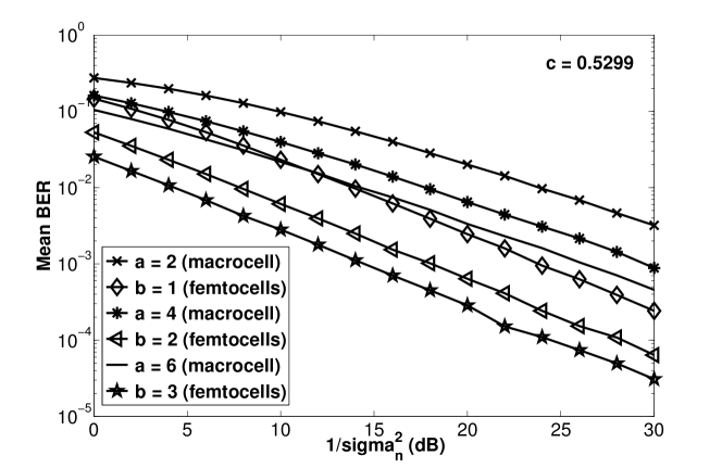
Figure 4: BER in macrocell and femtocells for different values of $a$ and $b$. As $a$ and $b$ increase BER performances in macrocell and femtocells improve.

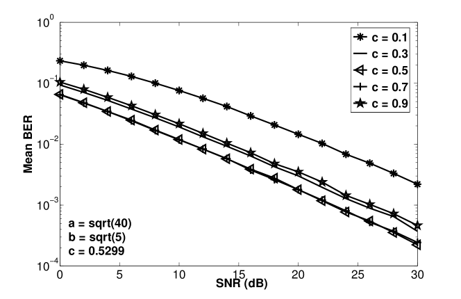
Figure 5: BER in the macrocell for different values of $c$. BER performance in the macrocell is improved for values of $c$ close to 0.5299.

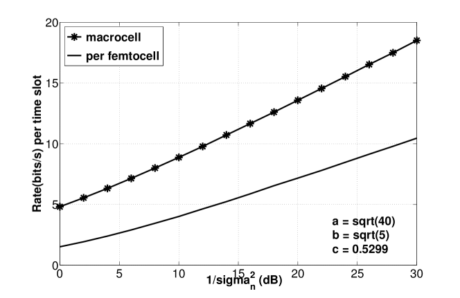
Figure 6: Rate of heterogeneous network with respect to the noise variance. The rate in the macrocell is higher than the rate per femtocell.

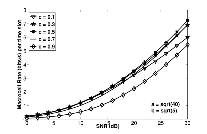
Figure 7: Rate in the macrocell for different values of $c$. The rate in the macrocell is optimised for values of $c$ very close to 0.5299.

V-B Sum Rate Performance

As discussed in section IV, the value of $c$ has a key-role in the sum rate performance of the macrocell. In Figure 6 the rate of the heterogeneous network is depicted and in Figure 7, it can be observed how the sum rate in the macrocell changes with $c$, achieving its best performance for values of $c$ close to $0.5299$.

VI Summary

Overall, this paper introduces how the BIA scheme can be applied into heterogeneous networks. Considering the fact that no CSIT is required, the DoF that can be achieved were discussed, which are the same with the IA scheme requiring perfect CSIT. Moreover, the BIA model was investigated from the perspective of equal power allocation, and how that can affect the optimal performance of the system. In that context, the important role of $c$, in the performance of the network, suggests that there is ground for further research on optimising the network performance. Finally, the description of the model in a Kronecker product representation provides a different insight on how the BIA scheme works.

VII Acknowledgements

This work was supported by NEC; the Engineering and Physical Sciences Research Council [EP/I028153/1]; and the University of Bristol. The authors thank Simon Fletcher & Patricia Wells for useful discussions.

References

- [1] M. Maddah-Ali, A. Motahari, A. Khandani, “Communications over X channel: Signaling and performance analysis”, in Tech. Report, UW-ECE-2006-12, University of Waterloo, July 2006.
- [2] V.R. Cadambe, S.A. Jafar, “Interference Alignment and Degrees of Freedom of the K-User Interference Channel”, IEEE Trans. Inf. Theory, vol. 54, no. 8, pp. 3425-3441, Aug. 2008.
- [3] O. El Ayach, S.W. Peters, R.W. Heath, “The Practical Challenges of Interference Alignment”, IEEE Wireless Commun., vol. 20, no. 1, pp. 35-42, Feb. 2013.
- [4] O.E. Ayach, S.W. Peters, R.W. Heath, “The Feasibility of Interference Alignment Over Measured MIMO-OFDM Channels”, IEEE Trans. Veh. Technol., vol. 59, no. 9, Nov. 2010.
- [5] T. Goum, C. Wang, S.A. Jafar, “Aiming Perfectly in the Dark-Blind Interference Alignment Through Staggered Antenna Switching”, IEEE Trans. Signal Process., vol. 59, no. 6, pp. 2734-2744, June 2011.
- [6] S.A. Jafar, “Blind Interference Alignment”, IEEE J. Sel. Topics Signal Proces., vol. 6, no. 3, pp. 216-227, June 2012.
- [7] S.A. Jafar, “Elements of Cellular Blind Interference Alignment-Aligned Frequency Reuse, Wireless Index Coding and Interference Diversity”, arXiv:1203.2384v1, Mar. 2012.
- [8] C. Wang, H.C. Papadopoulos, S.A. Ramprashad, G. Caire, ‘Design and Operation of Blind Interference Alignment in Cellular and Cluster-Based Systems’, ITA, Feb. 2011
- [9] C. Wang, H.C. Papadopoulos, S.A. Ramprashad, G. Caire, ‘Improved Blind Interference Alignment in a Cellular Environment using Power Allocation and Cell-Based Clusters’, IEEE ICC, Kyoto, June 2011