Kinematics of Clustering

Abstract

The dynamical system for inertial particles in fluid flow has both attracting and repelling regions, the interplay of which can localize particles. In laminar flow experiments we find that particles, initially moving throughout the fluid domain, can undergo an instability and cluster into subdomains of the fluid when the flow Reynolds number exceeds a critical value that depends on particle and fluid inertia. We derive an expression for the instability boundary and for a universal curve that describes the clustering rate for all particles.

1 Introduction

Dynamical systems theory is the natural language of transport. The kinematic equation $d\mathbf{x}/dt=\mathbf{u}(\mathbf{x},t)$ describes the Lagrangian motion of a passive particle at position $\mathbf{x}$ moving according to fluid velocity field $\mathbf{u}$, and for incompressible flows ($\nabla\cdot\mathbf{u}=0$) this is a volume-preserving dynamical system. Remarkably the physical coordinates of the fluid particles are exactly the same as the phase space coordinates of the dynamical system, permitting direct visualization of the system orbits, which can be regular or chaotic [3, 17, 10]. Particles, moving in fluids are often assumed to move passively if their inertia is small enough, tending toward neutrally buoyant and infinitesimally small. A particle moves passively when it does not change the fluid velocity field and instantaneously matches its own velocity to that of the fluid. How does the dynamical system for particle motion change in the presence of finite inertia?

Here we visualize the motion of inertial particles using a stirred tank laminar flow and examine a mechanism for particle localization that arises from interaction of the intrinsic inertia of particle and fluid. Stirred tanks are used globally in the processing industries and have been in industrial use almost unchanged for literally centuries [2]. The new result is the discovery and explanation of a particle clustering instability whereby particles moving initially through the entire fluid volume spontaneously move into and stay in a subdomain of the fluid. The explanation hinges on the existence and interplay of both attractors and repellors in the augmented dynamical system for motion of inertial particles. As attractors and repellors are caused by common features of natural or engineered flows, we anticipate that this localization mechanism may be activated in many laminar flows.

2 Inertial Particle Dynamical System

2.1 Fluid Motion

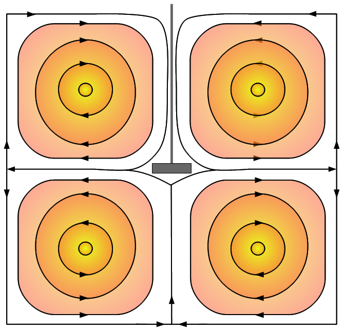
Unbaffled stirred tank flow is axisymmetric in time-average, and so produces a dynamical system that is 2-dimensional and conserves phase space. Figure 1a shows the skeleton of the laminar flow which has Kolmogorov–Arnold–Mosur (KAM) tubes above and below the impeller. The impeller provides a high frequency periodic perturbation to the flow skeleton to create a sea of chaotic orbits surrounding smaller KAM tubes (see figure 4). The boundaries of the KAM tubes are material surfaces, and fluid does not cross them, except by slow diffusion. This creates separated flow regions that do not exchange fluid. As stirred tanks are typically driven to turbulence, only recently have studies of the chaotic laminar flow in stirred tanks been reported [7, 18, 19].

2.2 Particle Motion

Newton’s law describing the velocity $\mathbf{V}_{p}(t)$ of a spherical particle with density $\rho_{p}$ and radius $a$ immersed in a fluid with density $\rho_{f}$ gives the Maxey–Riley (MR) equation of motion [9]:

$$\rho_{p}\frac{d\mathbf{V}_{p}}{dt} = \rho_{f}\frac{D\mathbf{u}}{Dt}+(\rho_{p}-\rho_{f})\mathbf{g}-\frac{9\nu\rho_{f}}{2a^{2}}\left(\mathbf{V}_{p}-\mathbf{u}\right)$$

$$-\frac{\rho_{f}}{2}\left(\frac{d\mathbf{V}_{p}}{dt}-\frac{D\mathbf{u}}{Dt}\right).$$

The forces are, respectively, the force exerted by the undisturbed flow on the particle, buoyancy force, Stokes drag and the added-mass from part of the fluid moving with the particle; neglected are the history force and higher order corrections [11]. There is a subtle difference between the operators $D/Dt$ and $d/dt$: $D/Dt=\partial/\partial t+\mathbf{u}\cdot\mathbf{\nabla}$ is the usual convective derivative taken along the path of a fluid element, while $d/dt=\partial/\partial t+\mathbf{V}_{p}\cdot\mathbf{\nabla}$ is a derivative taken along the particle trajectory. Both derivatives are the same for passive particles. Inertia is characterized by the parameter $\mu$,

$$\mu=\frac{St}{R}\quad\mbox{with}\quad R=\frac{2\rho_{f}}{\rho_{f}+2\rho_{p}}\quad\mbox{and}\quad St=\frac{2}{9}\left(\frac{a}{L}\right)^{2}Re,$$ (2)

where $St$ is the Stokes number, $R$ gives the density variation and Re is the flow Reynolds number; $\mu$ gives the ratio of the particle relaxation time and the typical time scale of the flow. Deviation of a particle from passive behavior is quantified by the particle Reynolds number $\mbox{{Re}}_{p}=a|\mathbf{V}_{p}-\mathbf{u}|/\nu$, $\nu$ the kinematic viscosity. $\mbox{{Re}}_{p}=0$ when a particle moves passively with the fluid and becomes non-zero when inertia causes particles to deviate from fluid streamlines: $\mbox{{Re}}_{p}\rightarrow 0$ as $\mu\rightarrow 0$.

Using (2f) to non-dimensionalize (2.2) gives

$$\mu\left(\frac{d\mathbf{V}_{p}}{dt}-\frac{3R}{2}\frac{D\mathbf{u}}{Dt}\right)=-\left(\mathbf{V}_{p}-\mathbf{u}\right),$$ (3)

where we have neglected buoyancy by setting gravity to zero; although, density differences are retained in $\mu$ through the added mass. Equation 3 is valid in the limit of dilute particle number density, $\mbox{{Re}}_{p}\ll 1$ and the assumption that particle motion does not effect $\mathbf{u}$, i.e. a one-way coupling. As our objective is the minimal model required to capture particle clustering, agreement with data must ultimately approve the approximations.

(a)	(b)

Figure 1: (a) Passive (fluid) particle dynamical system for stirred tank at low Re; two toroidal rolls exist above and below the impeller. (b) Phase space of augmented dynamical system for particle motion. Attracting hyperplane of fluid coordinates is perspective view of (a). Vertical coordinate is $\mbox{{Re}}_{p}$. Particle orbits repelled from the fluid hyperplane move in the full phase space and eventually reattract onto the hyperplane either outside tubes (blue) or inside tubes (red).

The addition of inertia augments the 2-dimensional fluid dynamical system to 4 dimensions in which the inertial particle trajectories move. The dynamical system for motion in the particle phase space $\mathbf{\chi}=(\mathbf{X}_{p},\mathbf{V}_{p})$ is

$$\frac{d\mathbf{X}_{p}}{dt}=\mathbf{V}_{p}$$ (4a)

$$\frac{d\mathbf{V}_{p}}{dt}=-\mu^{-1}\left(\mathbf{V}_{p}-\mathbf{u}\right)+\frac{3R}{2}\frac{D\mathbf{u}}{Dt}.$$ (4b)

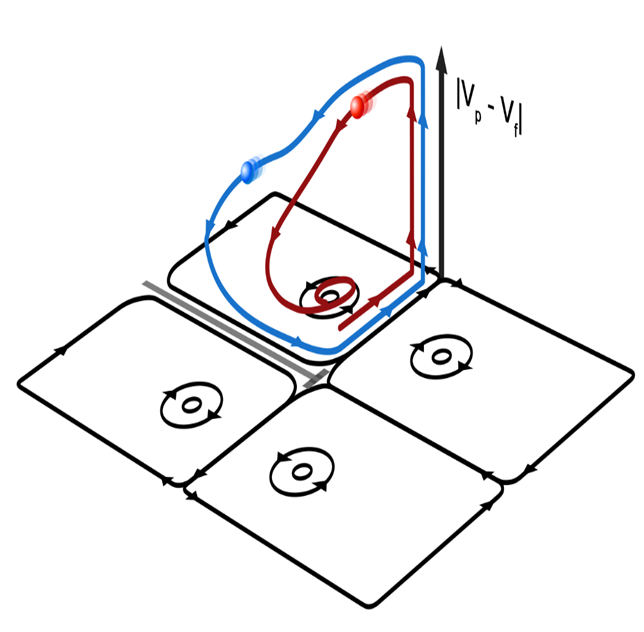
The inertial phase space has two key properties. (1) There is an attracting hyperplane containing passive fluid motion where $\mathbf{V}_{p}=\mathbf{u}$. This plane is overall attracting due to fluid drag, but in places this plane is repelling. Compact repelling regions are called repellors in contradistinction to attractors. (2) The system (4) is non-conservative with a divergence, the rate of contraction of phase space volume, given by

$$\nabla\cdot\mathbf{\chi}=-\mu^{-1}.$$ (5)

Non-conservation of phase volume is generic when other forces are added to the conservative fluid system [11].

Figure 1b schematically shows the phase space and representative orbits of the inertial dynamical system. The oblique plane is the fluid hyperplane and is the same as in figure 1a. Due to hydrodynamic drag, a particle will always eventually move nearly passively in the fluid hyperplane until perturbed away. When repelled from the fluid plane, a particle moves non-passively through the rest of the augmented dynamical system. This simply means that when a particle moves non-passively, it requires four numbers, the particle location and its velocity, to describe its state. Because the material surfaces of the separated flow regions are transport barriers only in the fluid plane, when particles leave the fluid plane and move through particle coordinate space (schematically shown in figure 1b with red and blue orbits), they can reattract to any part of the the fluid plane, ending up inside the separated flow region (red orbit) or outside of it (blue orbit). When attracted into separated flow regions that have no repellors, particles will stay in the attracting subdomains. This interplay between attracting and repelling flow regions can lead to particle clustering, as we demonstrate below.

3 Experiment

Figure 2: A tank, filled with moderately viscous fluid and particles, is stirred at a controlled rate by a Rushton impeller (view along shaft, top left corner). Light shines through a slit to illuminate a cross-section of flow which is filmed.

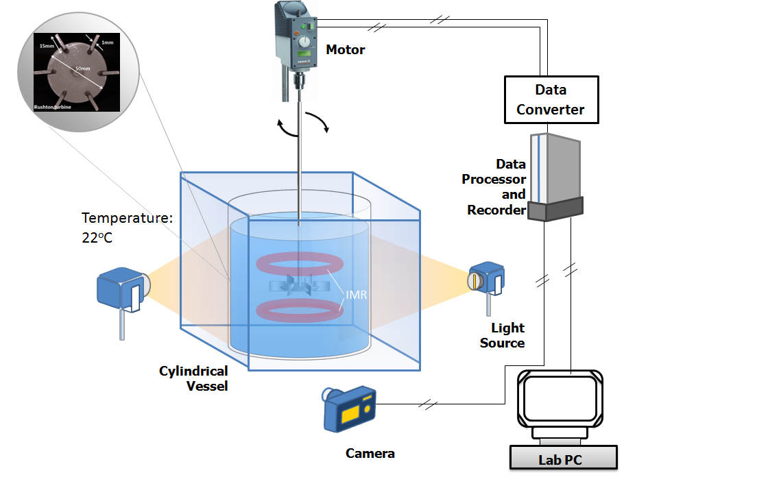
Our experiment (figure 2) consists of an open tank (190 mm diameter) filled (190 mm depth) with a moderately viscous fluid (1% water/glycerin; viscosity $\eta=0.83$ Pa-sec; density $\rho_{f}=1260$ kg/m³). Suspended by a centered shaft, half-way in the fluid depth, is an impeller (6-bladed Rushton) of a type that sucks fluid along the axial (shaft) directions and pushes fluid radially outward in the impeller plane. The impeller has a diameter $L=70$ mm and is rotated at a controlled rate $\Omega$; the flow Reynolds number is $\mbox{{Re}}=UL/\nu=\Omega L^{2}/\nu$, where $U=\Omega L$ and $L$ are the characteristic velocity and length scales of the fluid flow and $\nu=\eta/\rho_{f}$ is the kinematic viscosity. $\mbox{{Re}}<150$ here, an order of magnitude below the transition to turbulence.

3.1 Particles

particle	$a$	$\rho_{p}$	$\rho_{p}/\rho_{f}$	$a/L$	$\mu/\mbox{{Re}}$
	[mm]	kg/m3	—	$\times 10^{2}$	$\times 10^{4}$
Resin	$0.65\pm 0.05$	1220	0.97	0.93	0.28
Polystyrene	$1.4\pm 0.4$	1000	0.79	2.0	1.2
Polystyrene	$2.3\pm 0.4$	1000	0.79	3.3	3.1
PMMA	$3.18\pm 0.05$	1180	0.94	4.5	6.6
Capsule	$28\pm 0.05$	874	0.69	40	430

Table 1: Particle properties. Fluid density $\rho_{f}=1260$ kg/m³ and length scale $L=70$ mm. $\mu/\mbox{{Re}}$ is the intrinsic particle inertia, stripping out the variable component of fluid inertia

Particle properties are given in Table 1. The largest particle is the light capsule used for orbit visualization, described below. Experiments to measure the clustering instability boundary and the clustering rate use the other four particles. The light capsules used in figure 3 have $\mu\sim 1$, and the particles used to produce the data in Figs. 4 and 6 have $10^{-4}<\mu<10^{-2}$.

3.2 Visualization

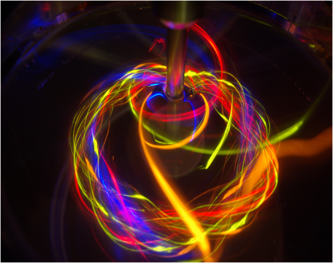(a)

(b)

Figure 3: Chaotic flow in a tank with impeller. Orbits visualized with long exposure photographs using light capsules of various colors. (a) Capsules started near the fluid surface, showing spontaneous migration of particles into a KAM tube. (b) Side view and close-up of impeller region; impeller not visible. Above and below impeller are KAM tubes in which particles execute helical orbits.

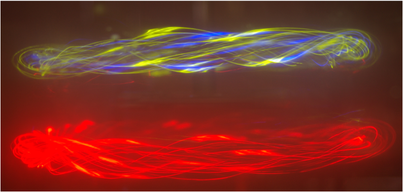
We visualize particle and fluid orbits in several ways. A new technique that we developed is particularly good at exposing the structure of individual orbits and is also suitable for larger containers. This method places a light emitting diode inside a transparent spherical capsule. Figure 3 shows long exposure photographs after one or a few light capsules were placed in the tank. Fig 3a is an oblique view from above and figure 3b is a side view. Above and below the impeller are the KAM tubes inside of which the light capsules trace out helical orbits. Outside the torus the pathlines of fluid particles are chaotic and well-mixed. The flow structure in the laminar flow tank is a typical chaotic flow with coexisting KAM and chaotic regions. This is the kinematic flow template that mediates the effects of inertial forces.

Several groups have examined particle motion inside laminar flow vortices [13, 20, 1] and found that particles migrate toward the center of a tube or, if cantori exist, particles may migrate into the cantori. Figure 3a shows orbits three capsules initially placed at the fluid surface that spontaneously and rapidly move through the chaotic region into the tube; once in the tube the capsules move in helical orbits passively with the fluid flow. Below we quantify and explain this type of particle localization using the four low inertia particles in Table 1. To our knowledge, our experiments are the first to show how inertial particles get into laminar flow vortex tubes.

4 Clustering Instability

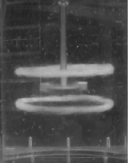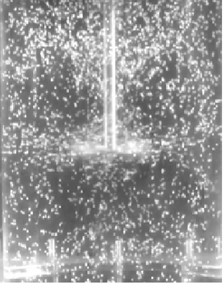
before instability	after instability

Figure 4: (right) After instability particle cluster into KAM tubes. (left) Before instability particles move throughout the tank except in KAM tubes.

Figure 4 illustrates the clustering transition. Flow is established at a particular Re, then particles are poured into the tank and swiftly disperse in the fluid everywhere except into the KAM tubes (figure 4a): particles move sufficiently passively to respect the material surface. At a somewhat higher Re we find that the particles spontaneously cluster into the tubes (figure 4b). There are two necessary conditions for particle clustering: (1) the existence of repellors to convert particle trajectories from being nearly coincident with fluid trajectories (passive behavior) into particle trajectories that are nearly independent of fluid trajectories (non-passive behavior); and, (2) separated flow regions, not too far away from repellors, into which particles can settle and that prevent particles from encountering repellors again. As condition (2) is amply fulfilled by the tubes of figure 3, we now specify condition (1) for a fluid repellor.

Prior to the work of Cartwright, Piro and co-workers [4, 5], it was commonly assumed that particles with low enough inertia would behave passively, i.e. a particle released in a fluid with a slight velocity mismatch compared to the fluid velocity (initially small $\mbox{{Re}}_{p}$) would adapt, after a short transient, to the local fluid velocity. If the right side of (3) is small, then the assumption appears natural to take $D/Dt=d/dt$, in which case (3) has the trivial solution that an initial velocity mismatch decays exponentially in a characteristic time of $\mu$. However, this is not always true. Sapsis and Haller [14, 8, 15], expanding on the earlier work [4, 5], proved that the fluid plane of (3) is overall attracting, but also that parts of the plane repel particles wherever

$$\sigma_{min}\left[\mathbf{S}+\mu^{-1}\mathbf{I}\right]<0.$$ (6)

$\mathbf{S}=\frac{1}{2}\left[\nabla\mathbf{u}+\left(\nabla\mathbf{u}\right)^{T}\right]$ is the rate of strain tensor, $\mathbf{I}$ is the unit tensor and $\sigma_{min}\left[\cdot\right]$ denotes the minimum eigenvalue of the bracketed tensor. As our flow is axisymmetric, the required eigenvalue can be determined from the characteristic equation of the $2\times 2$ matrix in (6) as $\sigma_{min}=\mu^{-1}-(-\det(\mathbf{S}))^{1/2}$. From a general result of matrix algebra, $-\det(\mathbf{S})=\frac{1}{2}\mathrm{tr}(S^{2})=\frac{1}{2}\mathbf{S}:\mathbf{S}$, where we have used that $\mathrm{tr}(\mathbf{S})=0$; the dyadic (double dot) product gives the sum of the squared strain rates along the eigendirections of $\mathbf{S}$. The invariant dyadic product of the rate of strain tensor is often used as the definition of the (local) total strain rate [6, 16], and we define the total strain rate as $\dot{\gamma}=\frac{1}{2}(\mathbf{S}:\mathbf{S})^{1/2}$, which converts (6) to

$$\mu\dot{\gamma}>1,$$ (7)

which we interpret as inertial stress. As the strain along streamlines is proportional to the radius of curvature of the streamline, a particle (nearly) passively follows a fluid streamline until the streamline curves too much, with (7) quantifying how much strain is “too much”. As a particle flows around the streamline curve, if the stress required to follow the fluid streamline exceeds (7), then inertial perturbations amplify particle trajectories away from fluid trajectories.

Strain rate varies with position in the fluid, and (7) is a local criterion. We estimate strain in the tank from the literature [12]. For Newtonian fluid $\dot{\gamma}=k\mbox{{Re}}$, where $k$ is a constant specific to impeller type. Equation 7 then becomes

$$\mu k>\mbox{{Re}}^{-1},$$ (8)

which is no longer a local quantity. Rather, it is an upper bound to the global instability boundary of critical Reynolds number for a particle with inertia $\mu$ to scatter from repellors.

Figure 5: Instability boundary theory and data. As a function of Re each particle type goes along a diagonal line with slope proportional to inertia. Thick line is (8). Open circles, no clustering; filled circles, clustering. For a Rushton impeller $k=5$.

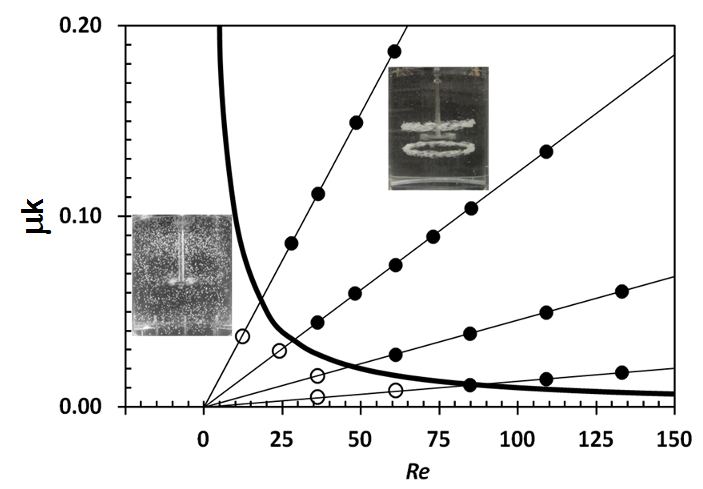
With the two necessary clustering conditions in hand, our experimental procedure is to introduce particles into the established flow at low Re, increase Re incrementally and film activity in the tank. Figure 5 plots data for four particles with $10^{-4}<\mu<10^{-2}$. Open circles denote no clustering and solid symbols clustering. As $St$ contains a factor of Re, each particle plots along a diagonal line with slope proportional to inertia. The thick solid line is (8). To the right and above the line, (8) predicts clustering, which is confirmed by the data. It is remarkable that the data agree so well with (8), which has no adjustable parameters.

5 Clustering Rate

Once a particle encounters repellor(s), it acquires a non-zero $\mbox{{Re}}_{p}$ and moves away from the fluid plane to move in the full inertial phase space (figure 1b). As the augmented dynamical system is non-conservative, the particle will reattract onto the fluid subspace, i.e. through drag the particle’s velocity and path will eventually approximate those of some fluid streamline until a repellor is again encountered. It is tempting to suppose that the clustering rate of particles into tubes is given by the divergence (5). The clustering rate should be proportional to the divergence; however, (5) is not the correct divergence because a repelled particle has $\mbox{{Re}}_{p}>1$ and the MR equation is no longer valid. Prediction of the rate of particle capture breaks down into two related questions: what is the probability $P_{c}$ of a particle being captured into a tube; and, what is the probability distribution $\cal P$ for the location in the fluid where a particle returns to moving passively?

(a)
(b)	(c)

Figure 6: Clustering rate. (a) Illustration of the probability density function ${\cal P}$ versus distance from a repellor. Vertical dashed lines illustrate a roll. (b) The increase of number of clustered particles as a function of time non-dimensionalized by the impeller rotation rate at the indicated inertia. Dots are data and lines are exponential fits. Cyan points are below the clustering threshold. (c) Data in (b) collapse onto a universal curve when time is scaled by the rate $\lambda$ defined in the text. Colors follow the legend in (b).

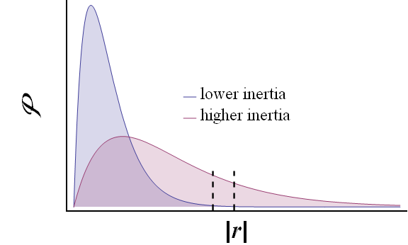
If $N_{t}$ is the number of particles that have gone into the tube, then the increase of $N_{t}$ during a time interval $dt$ is $dN_{t}=P_{c}\>dt$. The capture probability per unit time is proportional to the number of particles still outside the tube, $N_{f}$ (with the total number of particles $N_{0}=N_{f}+N_{t}$) and to the circulation rate of the flow. The capture probability is also proportional to the convolution of $\cal P$ with the tube volume fraction $\cal V$, which we have independently measured as a function of Re. Even in the absence of detailed knowledge of $\cal P$ we can still reach some general conclusions. Particles with less inertia will on average reacquire a fluid streamline closer to the repellor. With increasing particle inertia, $\cal P$ will spread out more evenly over the fluid domain. Figure 6a illustrates this idea, in which $|\mathbf{r}|$ is distance from the repellor and the dashed lines represent a separated region. From this line of reasoning we expect the clustering rate to increase with inertia. Of course, this illustration will be complicated by the possibility of more than one repellor. The capture probability per unit time $P_{c}\propto\Omega N_{f}\int{\cal P}{\cal V}\;dv$, where the convolution integral is taken over the fluid domain, and it follows that

$$\frac{dN_{t}}{d\tau}\propto\left(\frac{1}{2}N_{0}-N_{t}\right)\int{\cal P}{\cal V}\;dv,$$ (9)

where $\tau=\Omega t$ and the $1/2$ is from measuring the capture into a single tube whereas there are two tubes. Defining $w=N_{t}/(N_{0}/2)$, the solution to (9) is

$$w=1-\exp(-\lambda t).$$ (10)

$N_{t}$ is an exponential function of time that saturates at a rate $\lambda=\Omega\int{\cal P}{\cal V}\;dv$.

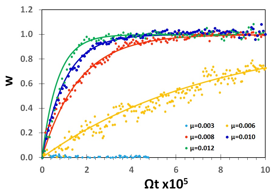
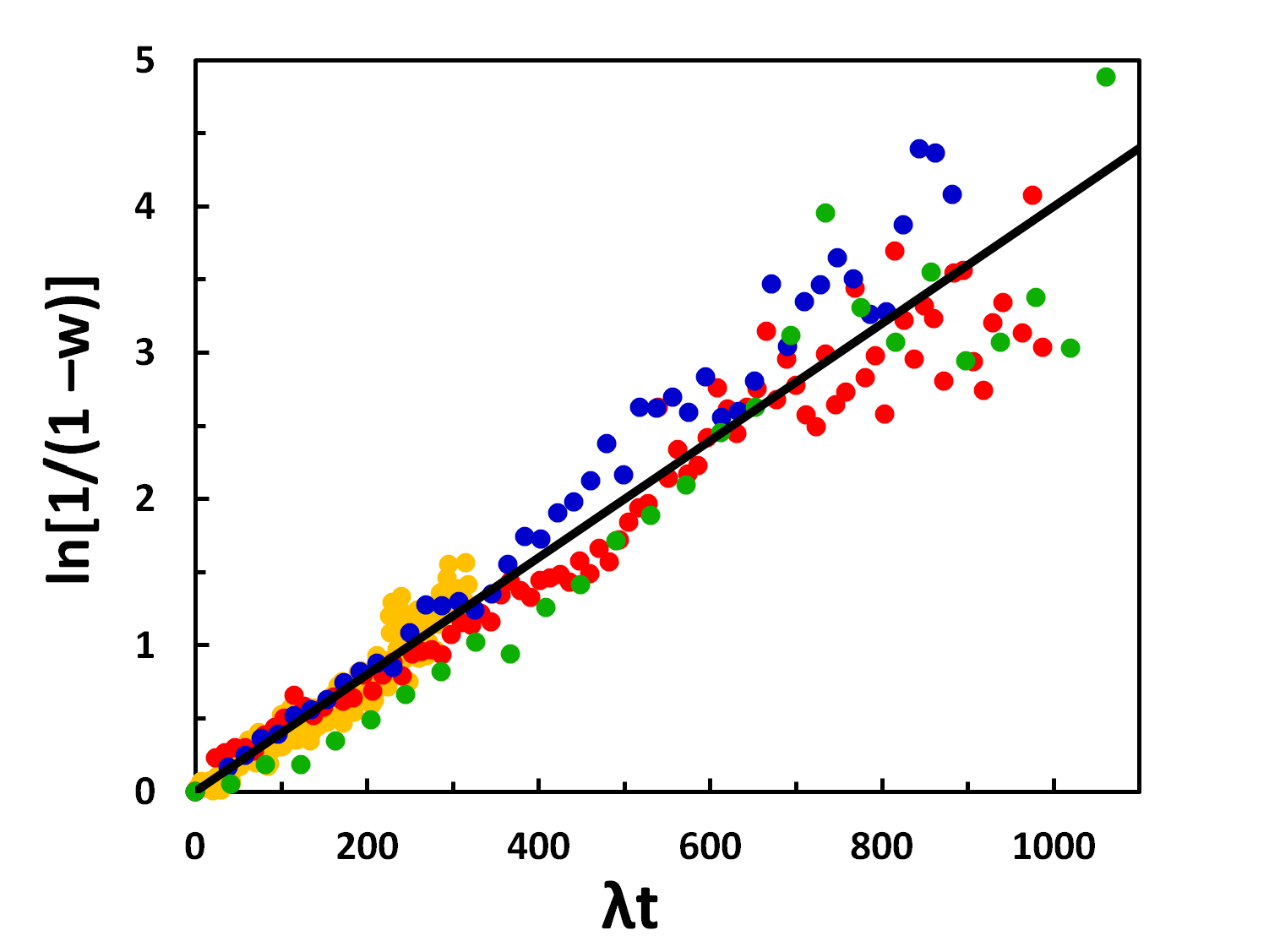
We test this prediction by measuring the number of particles captured by a tube $w$ as a function of time $t$. We do this by measuring the light transmitted through the region of a single tube and summing the pixel intensity. Figure 6b shows that $w$ is indeed a saturating exponential and that the clustering rate increases with $\mu$. We find that $\lambda=C(\mu-\mu_{c})^{\beta}{\cal V}\Omega$, with $\mu_{c}$ the value of $\mu$ at the instability boundary in figure 5, collapses all data onto a universal curve (figure 6c) with $\beta=1.79\pm 0.03$ and $C=(4.01\pm 0.04)\times 10^{-3}$.

6 Conclusions

We have outlined experiments and theory that pose some fresh answers to the question, where do particles go in fluid flows? As the ultimate fate, location and arrangement of particles is a key determinant of material form and function and of industrial process efficiency, this is a question that arises in diverse areas. Taking a dynamical systems approach, we have shown that the kinematics of inertial particles given by the MR equation has an augmented phase space with a hyperplane corresponding to passive fluid motion that both attracts and repels particles. The interplay of attractors and repellors can localize particles into small volumes of the fluid domain. Physically these involve respectively separated and sufficiently straining flow regions. Equation 8 gives the critical Re for when particle paths become divorced from fluid streamlines which is the onset of the clustering instability; the instability boundary depends only on material properties and the characteristic strain rate. MR kinematics accurately predicts how particles starting on the fluid manifold leave but cannot predict how particles reattract onto the fluid manifold. However, the clustering rate is well-characterized by a scaling relation. As the two necessary physical attributes are readily found in chaotic flows, we anticipate being able to activate this clustering instability in many flows.

Future work will take several approaches. First measurement or computation of the details of the velocity field would map out the location(s) and spatial extent of repellors. In the same vein direct measurement of the probability distribution $\cal P$ would be a difficult 3-dimensional experiment but could be done to understand the physics determining the clustering rate. Also, MR theory is restricted to spherical particles; extension of theory to non-spherical or deformable particles would be of great use. Finally, it has not escaped our notice that the clustering phenomena we have exposed suggests a basis for separation technologies.

References

- [1] Adetola A. Abatan, Joseph J. McCarthy, and Watson L. Vargas. Particle migration in the rotating flow between co-axial disks. AIChE Journal, 52(6):2039–2045, 2006.
- [2] Georgius Agricola. De Re Metallica. Dover Publications 1950, 1556. Book 8, image 22.
- [3] Hassan Aref. The development of chaotic advection. Physics of Fluids, 14(4):1315–1325, 2002.
- [4] Armando Babiano, Julyan Cartwright, Oreste Piro, and Antonello Provenzale. Dynamics of a small neutrally buoyant sphere in a fluid and targeting in Hamiltonian systems. Physical Review Letters, 84(25):5764–5767, 2000.
- [5] Julyan Cartwright, Marcelo Magnasco, and Oreste Piro. Bailout embeddings, targeting of invariant tori, and the control of Hamiltonian chaos. Physical Review, E 65:045203(R), 2002.
- [6] M. S. Chong, A. E. Perry, and B. J. Cantwell. A general classification of three-dimensional flow fields. Physics of Fluids, 2(5):765–777, 1990.
- [7] G. O. Fountain, D. V. Khakhar, I. Mezić, and J. M. Ottino. Chaotic mixing in a bounded three-dimensional flow. Journal of Fluid Mechanics, 417:265–301, 2000.
- [8] George Haller and Themistoklis Sapsis. Where do inertial particles go in fluid flows? Physica, D 237:573–583, 2008.
- [9] Martin R. Maxey and James J. Riley. Equation of motion for a small rigid sphere in a nonuniform flow. Physics of Fluids, 26:883–889, 1983.
- [10] Guy Metcalfe. Applied fluid chaos: Designing advection with periodically reoriented flows for micro to geophysical mixing and transport enhancement. In Robert L. Dewar and Frank Detering, editors, Complex physical, biophysical and econophysical systems, pages 187–239. World Scientific, 2010.
- [11] Guy Metcalfe, M. F. M. Speetjens, D. R. Lester, and H. J. H. Clercx. Beyond passive: Chaotic transport in stirred fluids. Advances in Applied Mechanics, 45:109–188, 2012.
- [12] Edward L. Paul, Victor Atiemo-Obeng, and Suzanne M. Kresta, editors. Handbook of Industrial Mixing. Wiley-Interscience, 2003.
- [13] Murray Rudman. Mixing and particle dispersion in the wavy vortex regime of Taylor-Couette flow. AIChE Journal, 44(5):1015–1026, 1998.
- [14] Themistoklis Sapsis and George Haller. Instabilities in the dynamics of neutrally buoyant particles. Physics of Fluids, 20:017102, 2008.
- [15] Themistoklis Sapsis and George Haller. Clustering criterion for inertial particles in two-dimensional time-periodic and three-dimensional steady flows. Chaos, 20:017515, 2010.
- [16] Michel Speetjens, Murray Rudman, and Guy Metcalfe. Flow regime analysis of non-Newtonian duct flows. Physics of Fluids, 18:013101, 2006.
- [17] R. Sturman, J. M. Ottino, and S. Wiggins. The Mathematical Foundations of Mixing. Cambridge University Press, 2006.
- [18] Koji Takahashi and Mitsunori Motoda. Chaotic mixing created by object inserted in a vessel agitated by an impeller. Chemical Engineering Research and Design, 87:386–390, 2009.
- [19] S. Wang, J. Wu, and E. Bong. Reduced IMRs in a mixing tank via agitation improvement. Chemical Engineering Research and Design, 91(6):1009–1017, 2013.
- [20] Steven T. Wereley and Richard M. Lueptow. Inertial particle motion in a Taylor Couette rotating filter. Physics of Fluids, 11(2):325–333, 1999.