Emission from Water Vapor and Absorption from Other Gases at 5–7.5 Microns in Spitzer-IRS Spectra of Protoplanetary Disks

Abstract

We present spectra of 13 T Tauri stars in the Taurus-Auriga star-forming region showing emission in Spitzer Space Telescope Infrared Spectrograph (IRS) 5–7.5$\mu$m spectra from water vapor and absorption from other gases in these stars’ protoplanetary disks. Seven stars’ spectra show an emission feature at 6.6$\mu$m due to the $\nu_{2}$ = 1–0 bending mode of water vapor, with the shape of the spectrum suggesting water vapor temperatures $>$500 K, though some of these spectra also show indications of an absorption band, likely from another molecule. This water vapor emission contrasts with the absorption from warm water vapor seen in the spectrum of the FU Orionis star V1057 Cyg. The other six of the thirteen stars have spectra showing a strong absorption band, peaking in strength at 5.6–5.7$\mu$m, which for some is consistent with gaseous formaldehyde (H₂CO) and for others is consistent with gaseous formic acid (HCOOH). There are indications that some of these six stars may also have weak water vapor emission. Modeling of these stars’ spectra suggests these gases are present in the inner few AU of their host disks, consistent with recent studies of infrared spectra showing gas in protoplanetary disks.

1 Introduction

Water has been observed in its gaseous form in numerous astrophysical environments. Its signature is seen in spectra of stellar atmospheres (Jørgensen et al., 2001; Jones et al., 2002; Roellig et al., 2004; Cushing et al., 2006), the extended atmosphere of Mira (Kuiper, 1962; Yamamura et al., 1999), and the circumstellar realms of numerous oxygen-rich Asymptotic Giant Branch stars (Cami, 2002; Sargent et al., 2010). The absorption and emission lines attributed to water in the 5.5–7.2$\mu$m Becklin-Neugebauer/Kleinman-Low (BN/KL) spectrum are identified as belonging to the $\nu_{2}$ = 1–0 bending mode of water vapor (Gonzalez-Alfonso et al., 1998). Spectral lines from water vapor were observed in spectra of the molecular cloud cores surrounding embedded Young Stellar Objects (YSOs; Helmich et al., 1996; van Dishoeck & Helmich, 1996; Dartois et al., 1998). Water vapor emission lines have been seen in the Spitzer Space Telescope (Werner et al., 2004) Infrared Spectrograph (IRS; Houck et al., 2004) spectra of the protostar NGC 1333-IRAS 4B (Watson et al., 2007).

Chiang & Goldreich (1997) noted that one of the most important coolants in young circumstellar disks is water vapor, and they discuss how gas may regulate the temperatures of dust grains in these disks. Observations of such protoplanetary disks are therefore crucial in helping to constrain the physics of such disks. Emission from water vapor has been seen in near-infrared (1 $<\lambda/\,{\rm\mu m}<$ 2.3) spectra of circumstellar disks (Carr et al., 2004) and in the far-infrared by Herschel-HIFI (Hogerheijde et al., 2011). Carr & Najita (2008) presented a mid-infrared Spitzer-IRS spectrum of the classical T Tauri star (TTS) AA Tau from 10–34 $\mu$m showing numerous emission lines from water vapor and the simple organic molecules HCN and C₂H₂. Numerous other studies (Mandell et al., 2008; Salyk et al., 2008; Pontoppidan et al., 2010a, b; Carr & Najita, 2011; Salyk et al., 2011; Mandell et al., 2012; Najita et al., 2013) have shown spectra indicating emission from these and other gases suggesting an origin in the inner few AU of protoplanetary disks. Najita et al. (2010) report HCO+ and possibly CH₃ from a Spitzer-IRS spectrum of TW Hya. These studies have typically made use of high-resolution Spitzer-IRS spectra; however, low-resolution Spitzer-IRS spectra have also been used to study molecular (including simple organic) emission (see studies of HCN and C₂H₂ by Pascucci et al., 2009; Teske et al., 2011). Here we report the detection of emission from water vapor (H₂O) and absorption from the simple organic molecules formaldehyde (H₂CO) and formic acid (HCOOH) in the inner regions of a number of TTSs in the Taurus-Auriga star-forming region as revealed by their 5–7.5$\mu$m spectra.

2 Data

2.1 Spectral Data Reduction

We analyze the spectra of 13 TTSs in the Taurus-Auriga star-forming region (Table 1). We selected the sources with the strongest emission or absorption structures in the 5–7.5 $\mu$m range not due to previously identified gas or solid-state species (e.g. polycyclic aromatic hydrocarbons – PAHs) or ices (Pontoppidan et al., 2005; Furlan et al., 2008; Zasowski et al., 2009; Boogert et al., 2011) from the Furlan et al. (2006) sample. All 5–7.5$\mu$m spectra included in our analysis were reduced and prepared by the same techniques (including dereddening) as described by Furlan et al. (2006) and Sargent et al. (2009), including deriving uncertainties from half the difference between the spectra obtained at the 2 nod positions, and applying a 1% lower threshold to the relative uncertainties, such that any relative uncertainty less than 1% was set to 1%. The spectra treated this way includes the spectrum of V1057 Cyg, a FU Orionis object whose spectrum was shown by Green et al. (2006) and suggested by those authors to have water vapor absorption bands over 5–7.5 $\mu$m wavelengths. Other spectra reduced and prepared this way include the Class III YSOs, HBC 388 and LkCa 1 (Furlan et al., 2006), which were chosen because they have no dust emission in excess of 2% of the continuum over 5–35 $\mu$m (i.e., the level of the flat field variation of the IRS; see the Spitzer-IRS Handbook), so any structure seen in their spectra must be photospheric in origin. As such, they are useful to compare to our TTS sample of 13 spectra.

2.2 Spectra with the 6.6$\mu$m Emission Feature

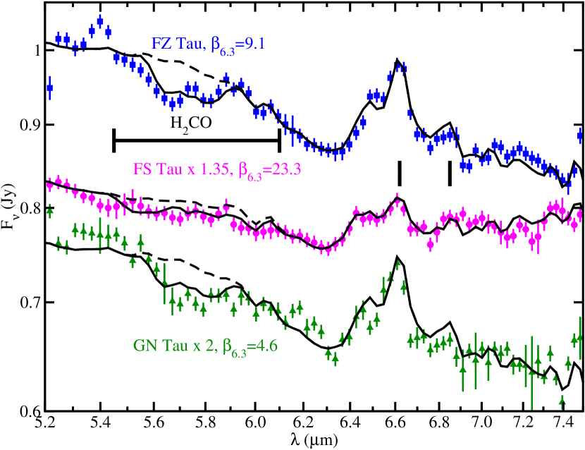
Figure 2: Spectra like RW Aur A, which show the 6.6$\mu$m water vapor emission feature but require H₂CO in the model. The data are solid points with one sigma error bars. FZ Tau is blue filled squares, FS Tau is magenta filled circles, and GN Tau is green upward-pointing triangles. The name of the star is indicated by the label of the same color as its spectrum. The black line going through each spectrum is the model of that spectrum. The amount by which the observed spectrum is scaled is indicated in the label for each source. The label also gives the ratio of the flux at 6.3$\mu$m in the observed spectrum to that inferred from the photosphere plotted for the source by Furlan et al. (2006), $\beta_{6.3}$. The two short vertical black lines have the same meaning as in Figure 1, as do the dashed lines and horizontal bar with vertical markers.

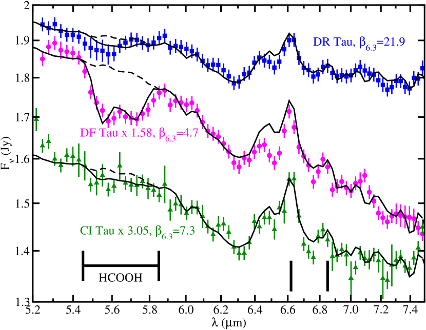
Figure 3: Spectra showing the 6.6 $\mu$m water vapor emission feature but requiring HCOOH in the model. Same plot convention as in Figure 2, except that DR Tau is the blue filled squares, DF Tau is the magenta filled circles, CI Tau is the green filled upward-pointing triangles, and the horizontal bar with vertical markers now indicates the wavelength span of the formic acid band.

The spectra of CI Tau, DF Tau, DR Tau, FS Tau, FZ Tau, GN Tau, and RW Aur A each show what appears to be an emission feature that peaks at ${\sim\,}$6.6$\mu$m. Figure 1 shows this feature for RW Aur A to be much larger in amplitude than the error bars on the data points composing the feature. The same is found for the other 6 spectra showing strong 6.6 $\mu$m emission features in Figures 2 and 3. In Table 1, we quantify the significance of the 6.6 $\mu$m feature by providing the ratio of the absolute value of the equivalent width of the feature to its uncertainty. For RW Aur A and the other 6 stars showing strong 6.6 $\mu$m emission features, this ratio is always greater than 8. In order to determine whether a feature was an artifact, we examined spectra of comparably bright TTSs, including DP Tau, AA Tau, FN Tau, GH Tau, and HK Tau (see Fig. 3 of Furlan et al., 2006), to determine the consistency of the 5–7.5 $\mu$m spectral band. The 5 comparison TTS spectra from Furlan et al. (2006) show hardly any spectral structure at all over these wavelengths; instead, one sees smooth continuum for these 5 spectra. All of the 13 TTS spectra we analyze in our study plus the 5 comparison TTS spectra from Furlan et al. (2006) have been reduced in a similar manner; e.g., variable column width aperture extraction, the use of RSRFs, etc. Therefore, we believe the 6.6$\mu$m emission features to be intrinsic to the TTSs and not artifacts.

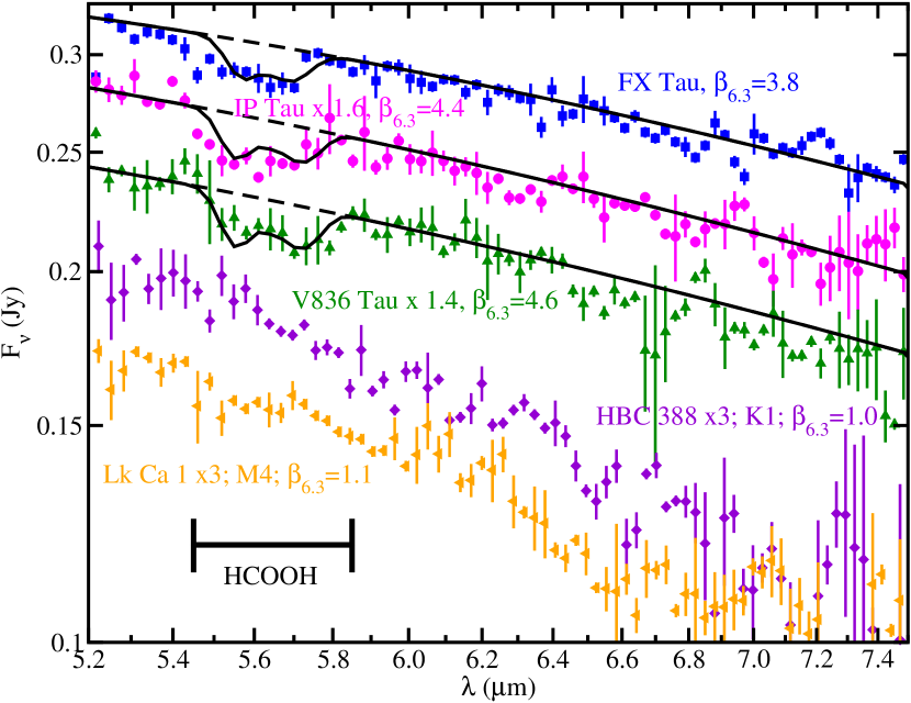
Figure 5: Spectra showing the 5.7 $\mu$m absorption band, modeled using HCOOH. Same plot convention as in Figure 2, except that FX Tau is the blue filled squares, IP Tau is the magenta filled circles, V836 Tau is the green upward-pointing filled triangles, and the horizontal bar with vertical markers now indicates the wavelength span of the formic acid band. Also shown are the Class III YSO sources HBC 388 as violet filled diamonds and Lk Ca 1 as orange filled leftward-pointing triangles.

The lack of this feature in Class III YSO spectra (e.g., see the spectra of HBC 388 and Lk Ca 1 in Figure 5) further argues against these features being artifacts. In general, the Short-Low detector of Spitzer-IRS (5–14 $\mu$m wavelength) is very well behaved, not suffering from the degree of the “rogue” pixel phenomenon (e.g., Watson et al., 2007) that, for example, the Long-High detector suffers. Finally, the degree of mispointing measured in the cross-dispersion direction (i.e., along the length of the slit) varies in our sample from less than 0.1 pixel width (the Short-Low pixel width is 1.8$\arcsec$) to 0.8 pixel width. As shown by Sargent (2009) for the Spitzer-IRS Mapping Mode observation of DH Tau, IQ Tau, and IT Tau (AOR # 3536128), the dispersion-direction (perpendicular to the length of the slit) mispointing tracked with the cross-dispersion mispointing. Therefore, mispointing of the observations does not seem to be responsible for the features seen at these wavelengths. It is also worth noting that some of these seven spectra showing strong 6.6 $\mu$m emission also have significant absorption in the 5.7 $\mu$m band. This includes FZ Tau, GN Tau, RW Aur A, and especially DF Tau. These four have 5.7 $\mu$m absorption band equivalent width to uncertainty ratios greater than 5 (see Table 1).

2.3 Spectra with the 5.7 $\mu$m Absorption Band

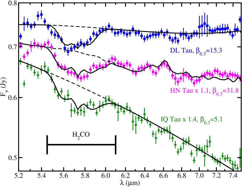
Figure 4: Spectra showing the 5.7 $\mu$m absorption band, modeled using H₂CO. Same plot convention as in Figure 2, except that DL Tau is the blue filled squares, HN Tau is the magenta filled circles, IQ Tau is the green filled upward-pointing triangles, and the horizontal bar with vertical markers now indicates the wavelength span of the formaldehyde band.

The spectra of DL Tau, FX Tau, HN Tau, IP Tau, IQ Tau, and V836 Tau each show what appears to be an absorption band centered around 5.7$\mu$m (Figures 4 and 5). As with the emission features in Figures 1, 2, and 3, Figures 4 and 5 show these absorption bands to be much larger in amplitude than the error bars on the data points composing the band. We computed the significance of this feature in a manner similar to how it was done for the 6.6 $\mu$m emission feature and provide it also in Table 1. Note that the significance of the 5.7 $\mu$m absorption band is always greater than 4. Also, two of these 5.7 $\mu$m absorption band exemplars, HN Tau and IP Tau, have 6.6 $\mu$m emission feature equivalent width to uncertainty ratios greater than 3 (Table 1). Thus, the presence of the 6.6 $\mu$m feature does not exclude the presence of the 5.7 $\mu$m band, and vice-versa.

3 Analysis

3.1 Models of the Seven Spectra with Strong 6.6 $\mu$m Emission Features

We argue that the 6.6 $\mu$m emission feature seen in the 5–7.5$\mu$m spectra of some of our sample arises from emission from water vapor, H₂O. Specifically, the water vapor emission seen over these wavelengths comes largely from the $\nu_{2}$ = 1–0 bending mode of water vapor, as in the case of the features seen by Gonzalez-Alfonso et al. (1998) in the spectrum of the BN/KL region of Orion. In the Gonzalez-Alfonso et al. (1998) BN/KL spectrum, the R branch ($\lambda<6.3\mu$m) lines are seen in absorption, the P branch ($\lambda>6.3\mu$m) lines are seen in emission; of the Q branch lines, some are in absorption, while others are in emission.

In Figure 1, we plot the spectrum and model of RW Aur A. We begin with RW Aur A to identify the most likely origin of the 6.6 $\mu$m feature. Our model includes water vapor only in emission. Full radiative transfer modeling is beyond the scope of the present work. We assume LTE for our models, and for RW Aur A, we assume a model with three components added together. We vary the temperature, column density, and inferred radius of emitting region to match the model to the data, judging the quality of fit by eye. We kept the model as simple as possible, but sufficiently complex so that the model fits the data well. The intensity of radiation emerging from each component is of the form

$$I_{\nu} = I_{\nu,0}e^{-\tau_{\nu}}+S_{\nu}(1-e^{-\tau_{\nu}})$$ (1)

where $I_{\nu,0}$ is the background intensity, $\tau_{\nu}$ is the optical depth of the slab of gas, and $S_{\nu}$ is the source function of the slab of gas (i.e., a Planck function at the temperature of the gas). We assumed the water vapor to have a microturbulent velocity of 1 km s^-1. Because of the low resolution of these Spitzer-IRS spectra, we have no information on the widths of the individual lines, as the water lines are not resolved, but our assumed microturbulent velocity is similar to the $\sigma$ = 2 km s^-1 local line width assumed by Salyk et al. (2008) for their gas modeling of Spitzer-IRS spectra of protoplanetary disks. The temperature of the water vapor giving rise to the 6.6 $\mu$m feature cannot be much lower than 500 K, or else the 6.6 $\mu$m feature would become too weak to match the spectrum. We used the HITEMP2010 line list for the main isotopologue of water vapor (Rothman et al., 2010), and the HITRAN2012 line list for the main isotopologue of formaldehyde (Rothman et al., 2013). For the partition function of these molecules at lower temperatures (T $\leq$ 75 K), we use the partition functions available at the Jet Propulsion Laboratory website (Pickett et al., 1998). For partition functions at higher temperatures, we use HITRAN2008 (Rothman et al., 2009). We then rebin the model to the spectral resolution of the IRS (R $\sim$ 60-120) over these wavelengths.

For RW Aur A, our model is a sum of the flux from 3 components, each of the form F_ν,i = $\Omega_{i}$I_ν,i, where the intensity, I_ν,i, for each is determined using Equation 1 (though some of the models use this equation iteratively to determine the emergent intensity for a more complicated geometry; see Section 3.2), each component with its own independent solid angle. The first component is an isothermal slab of water vapor at 1100 K of column density 1.7$\times$10¹⁵ cm^-2, with zero background intensity. The second component is a naked blackbody (i.e., no slab in front of it, so $\tau_{\nu}$ = 0) at 190 K. Both these two components have the same solid angle, which is equal to that of a face-on disk of radius 920$\,R_{\sun}$ at a distance of 139pc (the assumed distance to the Taurus/Auriga star-forming region; here, we follow Bertout et al., 1999). The third component features a 1400 K blackbody behind an isothermal cloud of formaldehyde (H₂CO) at 500 K of column density 7$\times$10¹⁸ cm^-2. The solid angle for the third component is equivalent to that of a face-on disk of radius 16.1$\,R_{\sun}$ at 139 pc. Though the solid angle for the water emission is much greater than that for the H₂CO absorption, the actual abundance ratio of the two (Table 2) is roughly 8:1 in favor of water. Perhaps the water giving rise to the spectral emission we see originates from a wider range of disk radii, while the formaldehyde originates from a narrower range. Because we do not perform self-consistent radiative transfer modeling of the gas emission and absorption, we cannot say much more about the relative locations in the protoplanetary disks of the water and the formaldehyde. The assumed column densities of water and formaldehyde are similar to or lower than the values for the molecules included in the model of AA Tau by Carr & Najita (2008) for wavelengths longward of 10 $\mu$m. Also, the solid angles of these components suggest regions in the inner few AU of the protoplanetary disk, consistent with the water vapor inferred from modeling by Carr & Najita (2008). That our model produces a 6.6$\mu$m emission feature means there must be a temperature inversion: the water vapor is hotter than the material underneath, further supporting an origin in the cooler disk regions in the inner few AU. The maximum optical depth of any of the H₂O lines in the model of RW Aur A over 5–7.5$\mu$m is $\sim$ 0.01, while the maximum optical depth of any of the H₂CO lines in the model is $\sim$ 4.4.

The model matches the 6.6 $\mu$m feature quite well, including the “shoulder” on the feature at 6.5 $\mu$m. Further, our model matches the overall shape of the 5–7.5 $\mu$m spectrum quite well, with only a few excursions outside of the spectral error bars. The water vapor emission in our model also matches the minor emission bump seen at 6.85 $\mu$m in the spectrum. We caution, however, that the “features” seen at 6.6 $\mu$m, 6.85 $\mu$m, etc are actually manifolds of multitudes of narrow water vapor lines that Spitzer-IRS cannot resolve at this low spectral resolution. For example, between 6.3 and 6.75 $\mu$m in the RW Aur A model (roughly corresponding to the 6.6 $\mu$m “feature”, or manifold), there are $>$ 500 lines of peak flux $>$ 0.05 Jy in the unconvolved model. Much of the water vapor emission seen over 5–7.5 $\mu$m belongs to the water vapor $\nu_{2}$ = 1–0 bending mode that Gonzalez-Alfonso et al. (1998) identified in their spectrum of BN/KL. Between 5.6–6.1 $\mu$m, the model is mostly within the error bars of the spectrum. The excursions over this range may be due to the simplicity of assuming absorption from formaldehyde at only one temperature (500 K). For our model of RW Aur A, we assume an abundance ratio of water to formaldehyde of $\sim$ 8 (Table 2). A range of temperatures of formaldehyde (see the models of DL Tau, HN Tau, and IQ Tau in Section 3.2) may improve the match of the model to the spectrum over this wavelength range.

As further verification of the identity of the species giving rise to the 6.6 $\mu$m feature, we model the spectrum of the FU Orionis object, V1057 Cyg. This star’s Spitzer-IRS spectrum was first presented by Green et al. (2006), who noted the presence of weak absorption bands between 5–7.5 $\mu$m in many of the FU Orionis type objects’ IRS spectra, including that of V1057 Cyg, and attributed these bands to water vapor. Indeed, Green et al. (2013) found emission from water in a Herschel-PACS spectrum of V1057 Cyg. Following the suggestion of Green et al. (2006), we constructed a model of water vapor absorption for this object’s spectrum. The first model component is an isothermal cloud of water vapor at 800 K of column density 6$\times$10¹⁹ cm^-2 in front of a 950 K blackbody subtending a solid angle equivalent to a face-on disk of radius 227 $\,R_{\sun}$ at a distance of 600pc (Hartmann & Kenyon, 1996), while the second model component is merely a 200 K blackbody subtending a solid angle equivalent to that of a face-on disk of radius 1800 $\,R_{\sun}$ at a distance of 600pc (Hartmann & Kenyon, 1996). For model details, see Table 2. The microturbulent velocity assumed for the water lines in the V1057 Cyg model is 10 km/s. The quality of the fit of the model to the V1057 Cyg spectrum is quite remarkable, considering the simplicity of the model. The model also matches the manifolds between 5.2–5.8 $\mu$m. In a number of ways the V1057 Cyg spectrum is a mirror of the RW Aur A spectrum: V1057 Cyg (RW Aur A) has a local maximum (minimum) at 6.3 $\mu$m, a shoulder at 6.5 $\mu$m, a local minimum (maximum) at 6.6 $\mu$m, a local minimum (maximum) at 6.8 $\mu$m, etc. One notable difference, however, is that the overall shape of the H₂O absorption band in the V1057 Cyg spectrum between 5.2–6.3 $\mu$m is not mirrored in a pure emission band in the RW Aur A spectrum. For comparison, a Spitzer-IRS spectrum of a pure H₂O emission band over these wavelengths can be seen in the spectrum of the lower-mass Oxygen-rich AGB star shown by Sargent et al. (2010). This supports our claim that there is absorption present in the RW Aur A spectrum at these wavelengths, and that formaldehyde is a good candidate to explain this.

We modeled the 6 other spectra showing strong 6.6 $\mu$m emission features in a manner similar to how we modeled RW Aur. The spectra and their best-fit models are shown in Figures 2 and 3, and the model parameters are listed in Table 2. We conclude water vapor emission is responsible for the 6.6 $\mu$m features seen in the observed spectra of RW Aur A (Figure 1) and the 6 other TTSs plotted in Figures 2 and 3.

For the spectra of FZ Tau, FS Tau, and GN Tau, we used models similar to that of RW Aur A, in that we used water and formaldehyde (Figure 2). As can be seen, the models match the observed data fairly successfully, matching the 6.6 $\mu$m feature well. The model of FZ Tau additionally successfully matches the $\sim$ 0.1 $\mu$m wide manifolds at 6.85, 5.7, 5.9, and 6.05 $\mu$m. Overall, the manifolds are weaker for FS Tau, and its model reflects that. Considering that the higher relative uncertainties on the data for GN Tau, the model fit is still satisfactory.

The spectra of DR Tau, DF Tau, and CI Tau require absorption from a molecule other than formaldehyde, as formaldehyde produces an absorption band too wide for these spectra, especially for DF Tau (Figure 3). Instead, for the models of these spectra, we replace formaldehyde with formic acid (HCOOH; line list for the main isotopologue from HITRAN2008; see Rothman et al., 2009). Again, the models match the spectra fairly successfully. For DF Tau, the formic acid absorption feature matches the absorption band very well in strength, width, central wavelength. It even matches the “dimple” at the bottom of the feature, around 5.65 $\mu$m. The model of DR Tau mostly matches the manifolds seen in its spectrum. The model of CI Tau also matches its spectrum well, though the relative uncertainties are somewhat higher than the other spectra in Figure 3.

3.2 Models of the Six Spectra with Strong 5.7 $\mu$m Absorption Bands

The other 6 TTS spectra in our sample of 13 show either weak 6.6 $\mu$m emission features or none at all. Rather, they show strong absorption bands centered at 5.7 $\mu$m. We note that these absorption bands are centered at too short a wavelength to be consistent with water ice absorption (see Pontoppidan et al., 2005). Organic ice mixtures are another possibility to consider. Such ices involve mixtures of H₂O, CH₃OH, NH₃, CO, CH₄, H₂CO, and other molecules, in varying ratios, both without and with ultraviolet photolysis, at varying temperatures (Greenberg, 1986; Allamandola et al., 1988; Schutte et al., 1993; Bernstein et al., 1994, 1995; Gerakines et al., 1996; Muñoz Caro & Schutte, 2003; Nuevo et al., 2006; Bisschop et al., 2007; Danger et al., 2013). The spectra of these organic ice mixtures are similar in that, though features begin appearing around 5.7 $\mu$m, the features grow stronger toward 10 $\mu$m wavelength. The same is true for kerogen and Murchison meteorite organic residue (Khare et al., 1990). The spectrum of H₂CO:NH₃ ice at 10 K after deposition shown by Schutte et al. (1993) is somewhat different in that its 5.8 $\mu$m feature is stronger than the other features out to 10 $\mu$m; however, the 5.8 $\mu$m does not match the central wavelengths of the absorption bands we observe in our TTS sample. Such behavior observed in the infrared spectra of all these studies of organic solids and ice mixtures is not observed in our spectra, so we do not attribute the 5.7 $\mu$m absorption in our TTS spectra to such organic solids and ice mixtures.

These 5.7 $\mu$m absorption bands are clearly seen in the spectra of DL Tau, HN Tau, IQ Tau, FX Tau, IP Tau, and V836 Tau (Figures 4 and 5) and are also seen for some of the stars showing the 6.6 $\mu$m emission feature (see previous subsection). For the model of RW Aur A (Figure 1 and Section 3.1), we modeled this absorption by including formaldehyde, H₂CO, in our model, in addition to water vapor. We do the same for HN Tau (Figure 4), as it seems to have a weak 6.6 $\mu$m emission feature. However, the 5–7.5 $\mu$m spectra of the other 5 spectra in Figures 4 and 5 seem to require no water vapor in their models.

Figure 4 shows the spectra and models of DL Tau, HN Tau, and IQ Tau. These models of DL Tau, HN Tau, and IQ Tau assume there is a layer of cold formaldehyde in front of a layer of warmer formaldehyde, in front of a hotter blackbody, and that the solid angle of the layers and blackbody are the same (Table 2). The model for HN Tau additionally includes a separate component of water vapor emission. In order to compute the part of the emergent spectrum giving rise to the absorption band, Equation 1 is used iteratively, such that the first iteration determines intensity I_ν from radiation emerging from the first layer, where the hot blackbody is I_ν,0, the source function of the lower (warmer) formaldehyde layer is S_ν, and $\tau_{\nu}$ is the optical depth of the lower formaldehyde layer. The intensity determined from this first iteration, I_ν, becomes the background intensity, I_ν,0, for the second iteration of Equation 1, where S_ν in the second iteration is the source function for the gas in the upper (cooler) formaldehyde layer, and $\tau_{\nu}$ in the second iteration is the optical depth of this upper formaldehyde layer. The warmer formaldehyde provides much of the absorption over the entire band, though less so at the center. The cooler formaldehyde provides the rest of the absorption at the center of the band. The maximum optical depth of any of the lines of formaldehyde over 5–7.5 $\mu$m comprising this model is ${\sim\,}$11. As noted previously, the absorption bands seen in our sample at these wavelengths seem to break down into two types: a wider band and a narrower band. The three spectra shown in Figure 4 have the wider band and are well modeled by formaldehyde. This wider band typically spans the region 5.4–6.0 $\mu$m.

The spectra of FX Tau, IP Tau, and V836 Tau, shown in Figure 5, have the narrower absorption band that is too narrow to be fit by formaldehyde, which fit the wider bands shown in Figure 4. This narrow band typically spans about 5.45–5.85 $\mu$m. For these 3 spectra, we assume absorption from formic acid instead of formaldehyde. As with the models in Figure 3, the formic acid produces a narrower band in each model shown in Figure 5 that mostly matches the observed absorption features. The best match is for V836 Tau, in terms of the width, strength, and central wavelength of the band, though the relative uncertainties are somewhat large. For IP Tau, the strength of the band is well modeled, though the model band is a little narrower and shifted slightly to longer wavelengths than the band seen in the data. The same is true for FX Tau, with a discrepancy between model and data perhaps slightly greater than was true for IP Tau.

We also include in Figure 5 the spectra of two Class III YSOs without any dust excess. These spectra - HBC 388, a K1 star, and LkCa 1, an M4 star - demonstrate that the photospheric contribution to any features seen at 5–7.5 $\mu$m is very minor, if present at all. The spectral types of these stars span most of the range of the spectral types for our sample of TTS (Table 1). HBC 388 shows hardly any absorption bands over these wavelengths at all. LkCa 1 shows a very shallow absorption band at 6.3–7 $\mu$m that is possibly due to water vapor in the stellar photosphere (Roellig et al., 2004; Cushing et al., 2006). However, excess infrared emission for our sample of TTSs essentially “fills in” such bands in the stellar photosphere spectra of our TTSs. The ratios of the observed flux at 6.3 $\mu$m (which, relatively free from water vapor lines, should give the best indication of the local dust continuum) to the inferred stellar photosphere flux (interpolated at this wavelength from the photospheric SEDs plotted for our TTS sample by Furlan et al., 2006) at this wavelength, $\beta_{6.3}$, are all very high, between 3.8 (FX Tau) and 31.8 (HN Tau; see Figures 4 and 5). Thus, the emission and absorption features and bands that we model in our TTS spectra are circumstellar in origin, not photospheric.

3.3 Equivalent Widths, Central Wavelengths, and Integrated Fluxes of the 5.7 $\mu$m Band and 6.6 $\mu$m Feature for Taurus-Auriga TTSs

We selected our sample of 13 TTSs from Taurus/Auriga because they showed the strongest 6.6 or 5.7 $\mu$m features. However, these features are seen in other TTS spectra from the Taurus/Auriga star-forming region. It is beyond the scope of the present study to model the emission seen in all such stars. However, it is relatively simple to measure the equivalent widths, central wavelengths (defined in the same sense as they were defined by Sloan et al., 2007), and integrated fluxes for our spectra. Equivalent widths provide a relative measure the strength of the emission or absorption features, while integrated fluxes provide an absolute measure of such strengths. The central wavelengths are important, especially for the 5.7 $\mu$m band because the central wavelength of the feature shifts according to the type of molecule providing the absorption (shorter central wavelength for formic acid, longer central wavelength for formaldehyde). Our modeling work informs these measurements by suggesting the wavelength ranges to fit continua and to measure central wavelength, equivalent width, or integrated flux.

We began by determining continua for the 6.6 and 5.7 $\mu$m features. We fit a power law continuum of the form F_ν,mod = 10${}^{C}\lambda^{P}$ to the data just outside each feature by least-squares; we used 5.36–5.429 and 6.026–6.10 $\mu$m for the 5.7 $\mu$m band and 6.265–6.34 and 6.7–7.0 $\mu$m for the 6.6 $\mu$m band. After determining the continuum to use for each feature, the equivalent width and integrated flux (defined as the difference between observed spectrum and computed continuum, integrated over the band) was computed over 5.428–6.026 $\mu$m for the 5.7 $\mu$m band and 6.34–6.7 $\mu$m for the 6.6 $\mu$m feature. We computed these equivalent widths and integrated fluxes for all the TTSs analyzed by Sargent et al. (2009) except for 4 – CoKu Tau/4, DM Tau, GM Aur, and Lk Ca 15 – as these TTSs have inner holes in their disks, so that there is little to no disk emission over 5–7.5 $\mu$m wavelength.

Next, we measured the central wavelengths of these features. To do this, we integrated, channel-by-channel across the features over the same wavelength ranges used to measure equivalent widths, from each end towards the other until we reached the first channel that put the channel integration sum over 50% of the total integrated flux within the feature. We then interpolated between this channel and the previous one to determine the wavelength corresponding to exactly 50% integrated flux. This was performed in both increasing and decreasing wavelength directions. The central wavelength is then the average of the result obtained from the two different directions.

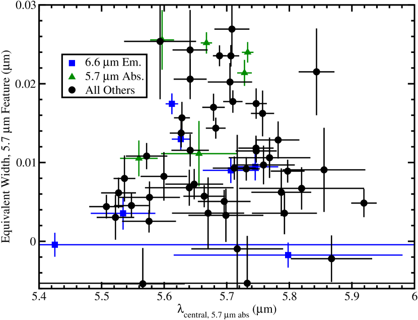
Figure 6: Plot of the measured 5.7 $\mu$m absorption feature equivalent width (in $\mu$m) versus the central wavelength of the 5.7 $\mu$m absorption feature. The blue filled squares are the 7 spectra in our sample showing strong 6.6 $\mu$m emission features, the green filled triangles are the 6 spectra in our sample showing strong 5.7 $\mu$m absorption features, and the black filled circles are the other 48 TTSs in the Sargent et al. (2009) sample (not including CoKu Tau/4, DM Tau, GM Aur, and Lk Ca 15 because they are transitional disks) from the Taurus/Auriga star-forming region.

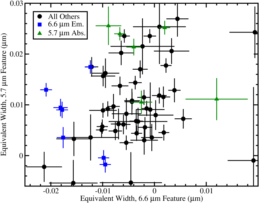
Figure 7: Plot of the measured 5.7 $\mu$m absorption feature equivalent width (in $\mu$m) versus the measured 6.6 $\mu$m emission feature equivalent width (in $\mu$m). Same plot style as in Figure 6.

We then searched for trends between the 5.7 and 6.6 $\mu$m central wavelengths and equivalent widths and the dust model parameters, stellar properties, and disk properties explored by Sargent et al. (2009), and also with the 5.7 and 6.6 $\mu$m central wavelengths, equivalent widths, and integrated fluxes themselves. The three H₂CO absorption exemplars (DL Tau, HN Tau, and IQ Tau; see Figure 4) do have 5.7 $\mu$m absorption band central wavelengths (5.668, 5.733, and 5.728 $\mu$m, respectively; see Table 1) systematically long-ward of the central wavelengths for the same band in the 3 HCOOH absorption exemplars (FX Tau, 5.560 $\mu$m; IP Tau, 5.597 $\mu$m; and V836 Tau, 5.656 $\mu$m; Figure 5; Table 1). However, very little in the way of significant correlations were found. Figure 6 shows the 5.7 $\mu$m equivalent width versus the 5.7 $\mu$m central wavelength. For smaller equivalent widths, there is a wide range of central wavelengths, but for the larger equivalent widths, the central wavelength ranges only between about 5.6–5.7 $\mu$m, which is consistent with the modeling described in Sections 3.1 and 3.2. We computed the correlation coefficient, r, and the probability of a correlation coefficient of equal or greater magnitude being found for a non correlated data set (Taylor, 1982), P, in the same manner as Sargent et al. (2009). We found r = 0.18 and P = 16% for the pair of 5.7 $\mu$m equivalent width and 5.7 $\mu$m central wavelength, so there is no correlation between this pair. We also searched for a trend between the 5.7 $\mu$m and 6.6 $\mu$m features’ equivalent widths. These are plotted in Figure 7. For this pair, we also find no correlation, with r = 0.24 and P = 6%.

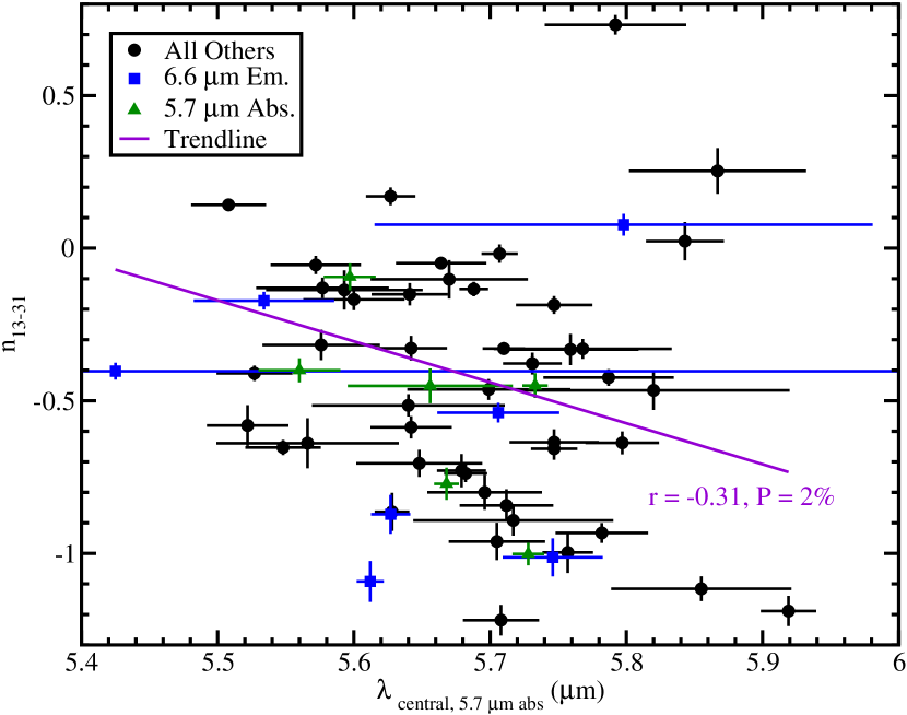
Figure 8: Plot of the 13-to-31 $\mu$m index versus the 5.7 $\mu$m absorption feature central wavelength. The trend line determined from least-squares fitting of all 59 plotted points is the violet line, and the correlation coefficient and probability of a correlation coefficient of equal or greater magnitude being found for a non-correlated data set (see Sargent et al., 2009) are indicated beside the line. Otherwise, same plot style as in Figure 6.

One pair that illustrates the typical sort of weak trend found between an equivalent width or central wavelength is between the spectral continuum index, n_13-31, measuring the continuum color in the infrared spectrum (Furlan et al., 2011), and the 5.7 $\mu$m central wavelength. This is plotted in Figure 8, with r = -0.31 and P = 2%, indicating there is a very weak indication of more negative 13-to-31 micron spectral index (bluer color) with increasing 5.7 $\mu$m central wavelength. However, at a glance, little correlation of note appears in Figure 8. More negative n_13-31 index suggests a more settled disk (Furlan et al., 2011). The trend would thus suggest that more settled disks tend to have the absorption band shifted to longer wavelengths, presumably because of greater H₂CO abundance relative to HCOOH. This potential trend should be explored in a larger sample of TTS spectra. Caution, however, is urged in attempting to interpret a correlation between n_13-31 index and 5.7 $\mu$m central wavelength.

3.4 Comparison of 6.6 $\mu$m Ro-vibrational and 17 $\mu$m Ground State H₂O Emission

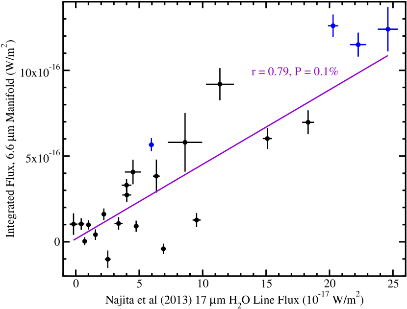
Figure 9: Plot of the 17 $\mu$m H₂O line flux (in 10^-17 W m^-2) from Najita et al. (2013) versus 6.6 $\mu$m emission manifold integrated flux (in W m^-2). Blue points are CI Tau, DR Tau, FZ Tau, and RW Aur A, as discussed in the text, while the black points are all the other stars in common between the Najita et al. (2013) sample and the sample for which we measured 6.6 and 5.7 $\mu$m equivalent widths and integrated fluxes. As with Figure 8, the violet line is the trend line, and the correlation coefficient and P are indicated beside the line.

Of the seven stars with strong H₂O emission (see Section 3.1), Najita et al. (2013) report $\sim$ 17 $\mu$m H₂O line fluxes from Spitzer-IRS Short-High ($\sim$ 10–19 $\mu$m) spectra for four: CI Tau, DR Tau, FZ Tau, and RW Aur A. By widening the comparison to all stars in common between the Najita et al. (2013) sample and all stars in our sample for which we measure equivalent widths and integrated fluxes, we obtain a sample of 23 stars. We plot in Figure 9 the 17 $\mu$m H₂O line fluxes from Najita et al. (2013) versus the 6.6 $\mu$m integrated fluxes we measure. There is a definite correlation between the Najita et al. (2013) 17 $\mu$m H₂O line flux with our 6.6 $\mu$m integrated fluxes of r = 0.79 and P = 0.1 %.

Carr & Najita (2011) note that H₂O lines in the 16–18 $\mu$m region are high-excitation ground state lines. Finzi et al. (1977) found that water relaxes from its stretching modes, $\nu_{1}$ and $\nu_{3}$, by first transferring to the bending overtone, $\nu_{2}$ = 2, then to the bending fundamental, $\nu_{2}$ = 1, then to the ground state; thus, the bending mode of water is strongly coupled to the rotational levels in the ground state (see also González-Alfonso & Cernicharo, 1999). The correlation between the rovibrational 5–7.5 $\mu$m H₂O emission and the 17 $\mu$m H₂O ground state lines could be consistent with non-LTE excitation of these H₂O ground state lines by radiative pumping through the H₂O $\nu_{2}$ = 1 mode. As Mandell et al. (2012) summarize, modeling by Meijerink et al. (2009) and observations by Mandell et al. (2008) and Pontoppidan et al. (2010a) suggest radiative pumping from the star enhances rovibrational H₂O emission from protoplanetary disks. We urge caution, however, as this sample size is somewhat small (23). In the future, we will compare the 6.6 $\mu$m H₂O feature to the 17 $\mu$m H₂O line fluxes in a larger sample.

4 Discussion

We note the temperatures required ($>$500 K) to fit the 6.6$\mu$m features in the 7 stars that have this feature are consistent with the temperature required to fit the $>$ 10–34 $\mu$m spectrum of AA Tau, 575 K, shown by Carr & Najita (2008). The water vapor in the circumstellar disk of AA Tau was inferred by Carr & Najita (2008) to arise from the inner regions of its disk ($<$ 3 AU). We similarly suggest the water vapor to be located in the inner regions of the protoplanetary disks whose spectra we show.

The H₂CO absorption exemplars, DL Tau, HN Tau, and IQ Tau, all seem to require 2 temperatures of H₂CO to fit their 5.7 $\mu$m absorption bands. As noted previously, the cooler 50 K component is added to “fill in” absorption at the center of the band that the warmer 500 K component could not do by itself. In reality, the H₂CO probably spans a range of temperatures in these disks, but we opt for simplicity in our modeling. The same is likely true for HCOOH and H₂O in our wider sample.

One point of comparison for our work is to the model of molecular emission by Carr & Najita (2011) from RW Aur A as seen in its high resolution Spitzer-IRS spectrum. Carr & Najita (2011) obtain a water temperature of 600 K, with a column density of water of 1.55$\times$10¹⁸cm^-2, and an inferred radius of emitting region of 1.49 AU. In our modeling, we determine a water temperature of 1100 K, a column density of 1.7$\times$10¹⁵cm^-2, and an inferred radius of emitting region of $\sim$ 4.3 AU. We model water lines over 5–7.5 $\mu$m wavelength, which arise mostly from $\nu_{2}$ = 1–0 transitions, while water lines at $\lambda>$ 10 $\mu$m modeled by Carr & Najita (2011) arise more from rotational transitions within the ground state of water. Thus, we likely probe different disk conditions. The water vapor in our model of RW Aur A has a lower column density spread out over a larger range of radii, so perhaps the hotter water vapor is located higher up in the atmosphere. Thermo-chemical modeling shows hot water vapor relatively high in the disk atmosphere ($>$1000 K gas located 1 AU above midplane at R = 3-4 AU from the star; see Figure 7 of Woitke et al., 2009). However, it is more likely that the higher resolution spectra modeled by Carr & Najita (2011) simply provide better constraints on the water vapor than the low resolution Short-Low 5–7.5 $\mu$m spectra we model. The higher resolution Spitzer-IRS spectra begin to separate emission lines (though such spectra do not necessarily outright resolve them), while Short-Low over 5–7.5 $\mu$m does not begin to resolve water emission lines.

Meijerink et al. (2009) suggest that protoplanetary disks that have experienced greater settling of dust to disk midplane, and therefore have higher gas-to-dust ratios in the upper disk layers, will have increased line-to-continuum ratios of emission from water vapor at infrared wavelengths. Furlan et al. (2006) compared spectral indices from radiative transfer models that include the effects of dust settling (D’Alessio et al., 2006) to observed spectral indices for TTSs in Taurus/Auriga and find that the mid-infrared continuum colors in general become bluer when there is greater dust settling and the disks become flatter. Furlan et al. (2011) measured the colors between 6–13 and 13–31 $\mu$m using the indices n_6-13 and n_13-31, which we cite for our sample in Table 1. Our sample’s n_6-13 indices range from -1.39 to -0.62, while our samples n_13-31 indices range from -1.09 to 0.03. As seen in Figure 7 of Furlan et al. (2011), such indices are consistent with a large fraction of the Taurus/Auriga TTS population, and as seen in Figure 22 of Furlan et al. (2011), this range of indices indicates significant settling, consistent with the suggestion by Meijerink et al. (2009). However, as we discussed in the previous subsection, we do not see trends between 6.6 $\mu$m equivalent width and either of the continuum color indices, n_6-13 and n_13-31. Perhaps any such trend is weak and might be found if our sample included more flared disks (i.e., with more positive indices).

We investigated the critical densities of the water vapor lines in the 5–7.5 $\mu$m region to determine how sensitive they might be to the degree of disk flaring (i.e., from dust settling) in protoplanetary disks. Using a list of energy levels for the ground (rotation-only) and first few vibrational states for both ortho- and para-water from Faure & Josselin (2008), we followed the methodology of Watson et al. (2007) and computed the sum of the Einstein A-coefficients of permitted downward radiative transitions and the sum of the collisional rate coefficients for H₂-H₂O (also from Faure & Josselin, 2008) for each possible level, and divided the former by the latter for each level. We determined the allowed transitions for the first few vibrational levels of water using the selection rules described by Thi & Bik (2005). From the Faure & Josselin (2008) collisional rate coefficients, we obtain critical densities of about 10⁷ to 10¹¹ cm^-3 for the first 45 levels (i.e., the ground state) of both ortho- and para-water. These values are somewhat lower than the 10¹⁰ to 10¹² cm^-3 determined by Watson et al. (2007) for water using levels and collisional rate coefficients from Green et al. (1993) and Phillips et al. (1996). Faure & Josselin (2008) note that their lower rates may be in error by up to 1 or 2 orders of magnitude, which perhaps helps explain this discrepancy. However, the Faure & Josselin (2008) collisional rate coefficients have the advantage of covering a wide range of transitions, and, thus, self-consistency. The lines in the 5–7.5 $\mu$m region giving rise, in large part, to the emission seen in our models that match the observed spectra are mostly $\nu_{2}$ = 1–0 transitions, though a few $\nu_{2}$ = 2–1 transitions also contribute. The critical densities of these lines assuming the Faure & Josselin (2008) collisional rate coefficients are in the range of about 10¹⁰ to 6$\times$10¹² cm^-3. Thus, the critical densities giving rise to the 5–7.5 $\mu$m water emission are, on average, an order of magnitude or two higher than those giving rise to the pure rotational transitions of water seen longward of 10 $\mu$m wavelength, suggesting the 5–7.5 $\mu$m water lines arise from denser disk regions. Thus, one might expect that the disks with least dust settling may hide their water vapor emission, assuming the scale height of the dust in the inner few AU of the disks increases sufficiently as a result of the increased flaring.

Our model of the FU Orionis star V1057 Cyg is interesting in that it lacks absorption from HCOOH or H₂CO, unlike the TTSs in our sample. Its spectrum is fit well with absorption only from H₂O at 800 K in front of a 950 K blackbody of radius 1.1 AU, with additional continuum emission from a 200 K blackbody of radius 8.4 AU. A glance at the spectra of other FU Orionis stars shown by Green et al. (2006) suggests they have absorption features in the 5–7.5 $\mu$m range largely or totally due to water vapor. Both having water vapor absorption instead of emission and lacking HCOOH and H₂CO absorption seems to differentiate this small sample of FU Orionis stars and our TTS sample. The water vapor absorption profiles of FU Orionis stars is likely due to internal heating from viscous accretion, while the water vapor emission profiles of TTS’s is likely due to external heating by stellar irradiation. The 5 FU Orionis stars studied by Green et al. (2006) are among the least extinguished (flat spectrum) FU Orionis stars by several different indices Green et al. (2013). Those with more extinction show absorption from various ices over the 5–7.5 $\mu$m range typical of Class 0/I protostars (Green et al., 2006; Quanz et al., 2007).

Qi et al. (2013) detected formaldehyde in the TTS disk of TW Hya and in the disk of the Herbig Ae star HD 163296 at millimeter wavelengths using the Submillimeter Array (SMA). They propose that formaldehyde may form from hydrogenation of CO ice. Aikawa et al. (2012) constructed psuedo-time-dependent models of molecules in a young protoplanetary disk, though it is not clear how these models perform concerning formaldehyde. Formic acid has been detected before from star-forming regions at radio wavelengths (Ikeda et al., 2001; Remijan & Hollis, 2006). Aikawa et al. (2012) also expect formic acid to play a significant role in disk chemistry. One major formation pathway for HCOOH gas comes from dissociative recombination of CH₃O${}_{2}^{+}$, which itself comes from a HCO⁺+H₂O reaction (Aikawa et al., 2012). It is also worth mentioning that formaldehyde (H₂CO) and formic acid (HCOOH) are chemically very similar, exchanging an H in formaldehyde for an OH in formic acid. Thus, it may be no coincidence that we see formaldehyde present in some TTS disks and formic acid in other TTS disks. We further note that both formaldehyde and formic acid ices are suggested by Spitzer-IRS spectra of Class I/II young stellar objects in the Taurus-Auriga star-forming region (Zasowski et al., 2009). Formaldehyde was also found in absorption in 3.6 $\mu$m spectra of the protostar W33A (Roueff et al., 2006). If these molecules are present in ices falling onto newly-formed protoplanetary disks, then they may also remain in the later phase when the envelope has finished falling onto the disk, for us to see in TTS spectra.

One possible explanation for the presence of formaldehyde gas in disks providing strong absorption is that the formaldehyde gas there is short-lived. Formaldehyde is known to undergo unimolecular dissociation (Troe, 2007). The rate coefficient, k_Mol,0, determined by Troe (2007) for formaldehyde dissociating to molecular hydrogen and CO is only valid between the temperatures of 1200–3500 K. We estimate the lifetime of formaldehyde in the disk of FZ Tau. Replacing the argon concentration in the Troe (2007) formula with an estimate of the disk gas density in its upper disk layers from the critical density of 10¹¹ cm^-3 determined by Watson et al. (2007) for the disk around the protostar NGC 1333 IRAS 4B (this value is in between the estimates of minimum and maximum gas density, n_min and n₀, respectively, at a radius of $\sim$ 3 AU in the disk model of Chiang & Goldreich, 1997), and assuming the disk gas is at the temperature of the H₂O (1200 K; see Table 2), we compute a half-life (the time it takes half of the population of this molecule to dissociate into molecular hydrogen and CO) of formaldehyde in the FZ Tau disk of $\sim$ 240 years. Such a short lifetime may provide a natural explanation for the general lower temperatures of formaldehyde in our models (Table 2) in that hotter formaldehyde molecules tend to dissociate and cease to exist, but we would advocate for more detailed follow-up calculations in the future.

5 Conclusions

We modeled the emission and absorption bands in the 5–7.5 $\mu$m region of 13 TTS in the Taurus-Auriga star-forming region. We show strong evidence for water vapor emission in the seven sources showing the 6.6$\mu$m emission feature. Such water emission contrasts with the absorption from water vapor seen in the spectrum of the FU Orionis star V1057 Cyg. It is remarkable how much of the spectral detail of the V1057 Cyg spectrum over 5–7.5 $\mu$m is matched by our model that includes absorption from water vapor at a single temperature of 800 K (with blackbodies providing continuum). For the entire sample, there is also absorption centered near 5.6-5.7$\mu$m that is consistent for some of the stars with formaldehyde and for others with formic acid. However, these are not the only stars in the Taurus/Auriga TTS population that show evidence of water vapor emission at 6.6$\mu$m or the absorption around 5.6–5.7$\mu$m from formaldehyde and/or some other gas species. Numerous Spitzer-IRS spectra of TTSs outside our present sample of 13 show a 6.6 $\mu$m emission feature and 5.7 $\mu$m absorption band (e.g., McClure et al., 2010; Furlan et al., 2011; Manoj et al., 2011).

For the TTS spectra requiring water vapor emission, the water vapor temperatures range between 600–1200 K, the column densities range from 1.7$\times$10¹⁵ cm^-2 to 3.6$\times$10¹⁷ cm^-2, and the inferred radii of the emitting region range from 200–1000 $\,R_{\sun}$ (Table 2). This results mostly in maximum optical depths for water lines between 5–7.5 $\mu$m mostly less than 1, except for DR Tau ($\tau_{max,1}\sim$ 5; Table 2). The cool blackbodies included to add longer wavelength continuum over this wavelength range go from 160–300 K.

The TTS spectra requiring formaldehyde absorption have formaldehyde temperatures ranging from 50–1000 K (sometimes they have formaldehyde at 2 temperatures), column densities ranging from 2$\times$10¹⁷ cm^-2 to 1.3$\times$10¹⁸ cm^-2, and inferred radii of the absorbing region ranging from 10–22 $\,R_{\sun}$. This results in formaldehyde 5–7.5 $\mu$m region maximum optical depths for any one component ranging from 2–11. The temperatures for the blackbody underlying these formaldehyde slabs range from 1000–1400 K; i.e., the hot inner regions of the disks (Table 2).

The TTS spectra requiring formic acid absorption have formic acid temperatures at either 500 or 1000 K, column densities ranging from 4$\times$10¹⁶ cm^-2 to 3.5$\times$10¹⁸ cm^-2, and inferred radii of the absorbing region ranging from 7 to 19 $\,R_{\sun}$. Maximum optical depths over 5–7.5 $\mu$m for any formic acid line range from 0.2–2.5. The blackbody underlying each formic acid slab ranges in temperature from 1300–1600 K, which (as with the blackbodies underlying the formaldehyde slabs) suggests an origin in the hot inner disk regions.

To confirm the identifications of formaldehyde and formic acid from the observed 5.6–5.7 $\mu$m absorption bands, we would suggest observations of nearby infrared bands of these molecules. Formic acid has the $\nu_{6}$ band centered near 9.05 $\mu$m (Baskakov et al., 2006) of approximately the same strength as the 5.65 $\mu$m band, as is revealed by the HITRAN2008 line list for formic acid (Rothman et al., 2009). There is a hint of shallow absorption near this wavelength as seen in the Spitzer-IRS spectrum of DF Tau (Sargent et al., 2009); however, this wavelength region is confused with emission from silicate dust. Therefore, it would be desirable to obtain high resolution N-band spectroscopy within the 8.75–9.25 $\mu$m range (approximately the span of the HCOOH 9.05 $\mu$m band) of stars whose Spitzer-IRS 5–7.5 $\mu$m spectra show absorption bands centered at 5.65 $\mu$m that are well-modeled by formic acid. Formic acid also possesses an additional band of comparable but slightly lesser strength centered near 15.6 $\mu$m (a blend of the $\nu_{7}$ and $\nu_{9}$ bands; see Baskakov et al., 2006). Lines have been computed for formic acid, however, at present, it appears that it is possible only to compute relative line intensities for this band (Perrin et al., 2002). There are also weaker bands of formic acid centered near 2.8 and 3.4 $\mu$m ($\nu_{1}$ and $\nu_{2}$, respectively Baskakov et al., 2006), but we could not find any line data for them. For formaldehyde, there is a band of comparable strength to the 5.7 $\mu$m band centered near 3.55 $\mu$m. This was the band whose lines were observed by Roueff et al. (2006) in the infrared spectrum of the protostar W33A. There are no other infrared bands of comparable strength to these two bands for formaldehyde, so we would advocate high resolution L-band ($\sim$ 3.55 $\mu$m) observations of stars whose Spitzer-IRS spectra show a 5.7 $\mu$m absorption band that is best modeled by formaldehyde, to confirm the presence of formaldehyde based on the 5.7 $\mu$m band.

Spectral data at 5–7.5$\mu$m will be quite powerful when combined with data on water vapor and other gases longward of 10$\mu$m, like what Carr & Najita (2008) showed and modeled for AA Tau. Additionally, data on water vapor, when combined with data on CO (see Najita et al., 1996, 2003), OH (Mandell et al., 2008), etc., promises to reveal much about the physics and chemistry of gases in protoplanetary disks. Higher-resolution spectroscopic follow-up by current missions, such as SOFIA, and future missions such as James Webb Space Telescope (JWST) should begin to separate the lines of water vapor, formaldehyde, formic acid, and other gas species in the 5–7.5$\mu$m region of these stars’ spectra. Using these observations, detailed modeling should yield valuable clues regarding the origin of water in the inner regions of protoplanetary disks, which is relevant to studies of the origin of water on planets in the habitable zones of stars.

Figure 1: Detailed model of the spectra of RW Aur A (a TTS) and V1057 Cyg (an FU Ori star). The observed spectrum of RW Aur A is the black filled circles with one sigma error bars. The green line is the model for RW Aur A. The blue filled squares and associated one sigma error bars are the spectrum of V1057 Cyg, and the orange solid line is the model of this spectrum. Both model and spectrum for V1057 Cyg are scaled by 0.29. For details, see Section 3.1 of the text. The two short vertical black lines indicate the central wavelengths of the 6.6 and 6.85 $\mu$m emission features discussed in the text. The dashed line is a model of RW Aur A that is the same as the solid line model, except that there is no formaldehyde absorption. The horizontal bar with vertical markers labeled H₂CO indicates the wavelength span of the formaldehyde band.

Table 1: Sample

	Sp.			Misptg.	Misptg.	5.7$\mu$m	5.7$\mu$m	5.7$\mu$m	6.6$\mu$m	6.6$\mu$m	6.6$\mu$m
Star	Ty.a	n${}_{6-13}^{\rm a}$	n${}_{13-31}^{\rm a}$	SL2n1b	SL2n2b	$\lambda_{central}^{c}$	EW$\times$1000d	$\left|EW\right|$/$\sigma_{EW}^{e}$	$\lambda_{central}^{c}$	EW$\times$1000d	$\left|EW\right|$/$\sigma_{EW}^{e}$
6.6 $\mu$m Emissionf
CI Tau	K7	-0.97	-0.17	0.062	-0.096	5.534$\pm$0.052	3.55$\pm$2.1	1.7	6.573$\pm$0.012	-17.6$\pm$1.2	15
DF Tau	M2	-1.39	-1.09	$\cdots$	$\cdots$	5.612$\pm$0.010	17.5$\pm$1.3	13	6.597$\pm$0.007	-12.4$\pm$1.1	11
DR Tau	K5	-0.90	-0.40	$\cdots$	$\cdots$	5.425$\pm$1.529	-0.4$\pm$1.5	0.27	6.574$\pm$0.014	-9.8$\pm$1.1	8.9
FS Tau	M0	-0.62	0.03	-0.075	0.096	5.798$\pm$0.183	-1.7$\pm$1.6	1.1	6.529$\pm$0.023	-9.5$\pm$1.1	8.6
FZ Tau	M0	-1.18	-0.89	0.363	0.768	5.627$\pm$0.014	13.0$\pm$1.3	10	6.582$\pm$0.006	-20.9$\pm$1.1	19
GN Tau	M2.5	-0.96	-1.02	$\cdots$	$\cdots$	5.746$\pm$0.037	9.5$\pm$1.7	5.6	6.572$\pm$0.007	-18.1$\pm$1.4	13
RW Aur A	K3	-0.69	-0.54	$\cdots$	$\cdots$	5.706$\pm$0.045	9.0$\pm$1.6	5.6	6.580$\pm$0.007	-17.8$\pm$1.1	16
5.7 $\mu$m Absorptionf
DL Tau	K7	-0.77	-0.77	-0.662	-0.278	5.668$\pm$0.009	25.2$\pm$1.4	18	6.425$\pm$0.044	2.0$\pm$1.1	1.8
FX Tau	M1	-1.07	-0.40	0.095	0.315	5.560$\pm$0.030	10.5$\pm$2.3	4.6	6.551$\pm$0.063	-2.5$\pm$2.1	1.2
HN Tau	K5	-0.70	-0.44	$\cdots$	$\cdots$	5.733$\pm$0.009	24.0$\pm$1.3	18	6.572$\pm$0.018	-6.7$\pm$1.1	6.1
IP Tau	M0	-0.93	-0.11	0.335	0.132	5.597$\pm$0.019	25.6$\pm$3.8	6.7	6.481$\pm$0.021	-8.9$\pm$2.5	3.6
IQ Tau	M0.5	-1.30	-1.00	-0.248	-0.61	5.728$\pm$0.012	21.4$\pm$1.6	13	6.528$\pm$0.047	-4.0$\pm$1.4	2.9
V836 Tau	K7	-1.38	-0.45	$\cdots$	$\cdots$	5.656$\pm$0.061	11.1$\pm$4.1	2.7	6.662$\pm$0.031	12.0$\pm$6.0	2.0

Table 2: Models

H2O						H2CO or HCOOH
	T1	N1	Tbb1	R${}_{bb1}^{a}$		T2	N2	Tbb2	R${}_{bb2}^{a}$		abund.
Star	(K)	(1018 cm-2)	(K)	(AU)	$\tau_{max,1}$	(K)	(1018 cm-2)	(K)	($\,R_{\sun}$)	$\tau_{max,2}$	ratiob
H2O and H2CO
DL Tauc	$\cdots$	$\cdots$	200	2.0	$\cdots$	300,50	1.1,0.2	1000	22	10,7.0	0
FS Tau	600	0.01	200	2.5	0.13	1000	1	1400	13	2.3	18
FZ Tau	1200	0.005	190	2.5	0.026	150	0.8	1400	16	14	6.7
GN Tau	1100	0.01	200	1.2	0.058	200	0.5	1400	10	6.7	13
HN Tauc	900	0.0035	200	1.8	0.026	500,50	1.3,0.3	1200	16	8.2,11	1.4
IQ Tauc	$\cdots$	$\cdots$	$\cdots$	$\cdots$	$\cdots$	500,50	1.2,0.2	1400	11	7.5,7.0	0
RW Aur A	1100	0.0017	190	4.3	0.0099	500	0.7	1400	16	4.4	7.9
H2O and HCOOH
CI Tau	900	0.0085	200	1.6	0.062	1000	0.5	1400	12	0.35	15
DF Tau	900	0.0022	160	4.7	0.016	1000	3	1400	18	2.1	2.3
DR Tau	600	0.36	300	0.93	4.6	500	0.04	1600	19	0.22	980
FX Tau	$\cdots$	$\cdots$	$\cdots$	$\cdots$	$\cdots$	500	0.2	1300	10	1.1	0
IP Tau	$\cdots$	$\cdots$	$\cdots$	$\cdots$	$\cdots$	1000	2.8	1400	6.9	2.0	0
V836 Tau	$\cdots$	$\cdots$	$\cdots$	$\cdots$	$\cdots$	1000	3.5	1400	6.8	2.5	0
H2O Only
V1057 Cygd	800	60	200	8.4	74	$\cdots$	$\cdots$	$\cdots$	$\cdots$	$\cdots$	$\infty$

References

- Aikawa et al. (2012) Aikawa, Y., Wakelam, V., Hersant, F., Garrod, R. T., & Herbst, E. 2012, ApJ, 760, 40
- Allamandola et al. (1988) Allamandola, L. J., Sandford, S. A., & Valero, G. J. 1988, Icarus, 76, 225
- Baskakov et al. (2006) Baskakov, O. I., Markov, I. A., Alekseev, E. A., et al. 2006, Journal of Molecular Structure, 795, 54
- Bernstein et al. (1994) Bernstein, M. P., Sandford, S. A., Allamandola, L. J., & Chang, S. 1994, Journal of Physical Chemistry, 98, 12206
- Bernstein et al. (1995) Bernstein, M. P., Sandford, S. A., Allamandola, L. J., Chang, S., & Scharberg, M. A. 1995, ApJ, 454, 327
- Bertout et al. (1999) Bertout, C., Robichon, N., & Arenou, F. 1999, A&A, 352, 574
- Bisschop et al. (2007) Bisschop, S. E., Fuchs, G. W., Boogert, A. C. A., van Dishoeck, E. F., & Linnartz, H. 2007, A&A, 470, 749
- Boogert et al. (2011) Boogert, A. C. A., Huard, T. L., Cook, A. M., et al. 2011, ApJ, 729, 92
- Cami (2002) Cami, J. 2002, Ph.D. Thesis,
- Carr et al. (2004) Carr, J. S., Tokunaga, A. T., & Najita, J. 2004, ApJ, 603, 213
- Carr & Najita (2008) Carr, J. S., & Najita, J. R. 2008, Science, 319, 1504
- Carr & Najita (2011) Carr, J. S., & Najita, J. R. 2011, ApJ, 733, 102
- Chiang & Goldreich (1997) Chiang, E. I., & Goldreich, P. 1997, ApJ, 490, 368
- Cushing et al. (2006) Cushing, M. C., et al. 2006, ApJ, 648, 614
- D’Alessio et al. (2006) D’Alessio, P., Calvet, N., Hartmann, L., Franco-Hernández, R., & Servín, H. 2006, ApJ, 638, 314
- Danger et al. (2013) Danger, G., Orthous-Daunay, F.-R., de Marcellus, P., et al. 2013, Geochim. Cosmochim. Acta, 118, 184
- Dartois et al. (1998) Dartois, E., D’Hendecourt, L., Boulanger, F., Jourdain de Muizon, M., Breitfellner, M., Puget, J.-L., & Habing, H. J. 1998, A&A, 331, 651
- Faure & Josselin (2008) Faure, A., & Josselin, E. 2008, A&A, 492, 257
- Finzi et al. (1977) Finzi, J., Hovis, F. E., Panfilov, V. N., Hess, P., & Moore, C. B. 1977, J. Chem. Phys., 67, 4053
- Furlan et al. (2006) Furlan, E., et al. 2006, ApJS, 165, 568
- Furlan et al. (2008) Furlan, E., McClure, M., Calvet, N., et al. 2008, ApJS, 176, 184
- Furlan et al. (2011) Furlan, E., Luhman, K. L., Espaillat, C., et al. 2011, ApJS, 195, 3
- Gerakines et al. (1996) Gerakines, P. A., Schutte, W. A., & Ehrenfreund, P. 1996, A&A, 312, 289
- Gonzalez-Alfonso et al. (1998) Gonzalez-Alfonso, E., Cernicharo, J., van Dishoeck, E. F., Wright, C. M., & Heras, A. 1998, ApJ, 502, L169
- González-Alfonso & Cernicharo (1999) González-Alfonso, E., & Cernicharo, J. 1999, ApJ, 525, 845
- Green et al. (1993) Green, S., Maluendes, S., & McLean, A. D. 1993, ApJS, 85, 181
- Green et al. (2006) Green, J. D., Hartmann, L., Calvet, N., et al. 2006, ApJ, 648, 1099
- Green et al. (2013) Green, J. D., Evans, N. J., II, Kóspál, Á., et al. 2013, ApJ, 772, 117
- Greenberg (1986) Greenberg, J. M. 1986, Ap&SS, 128, 17
- Hartmann & Kenyon (1996) Hartmann, L., & Kenyon, S. J. 1996, ARA&A, 34, 207
- Helmich et al. (1996) Helmich, F. P., et al. 1996, A&A, 315, L173
- Hogerheijde et al. (2011) Hogerheijde, M. R., Bergin, E. A., Brinch, C., et al. 2011, Science, 334, 338
- Houck et al. (2004) Houck, J. R., et al. 2004, ApJS, 154, 18
- Ikeda et al. (2001) Ikeda, M., Ohishi, M., Nummelin, A., et al. 2001, ApJ, 560, 792
- Jones et al. (2002) Jones, H. R. A., Pavlenko, Y., Viti, S., & Tennyson, J. 2002, MNRAS, 330, 675
- Jørgensen et al. (2001) Jørgensen, U. G., Jensen, P., Sørensen, G. O., & Aringer, B. 2001, A&A, 372, 249
- Khare et al. (1990) Khare, B. N., Thompson, W. R., Sagan, C., et al. 1990, First International Conference on Laboratory Research for Planetary Atmospheres, 3077, 340
- Kuiper (1962) Kuiper, G. P. 1962, Communications of the Lunar and Planetary Laboratory, 1, 197
- Mandell et al. (2008) Mandell, A. M., Mumma, M. J., Blake, G. A., Bonev, B. P., Villanueva, G. L., & Salyk, C. 2008, ApJ, 681, L25
- Mandell et al. (2012) Mandell, A. M., Bast, J., van Dishoeck, E. F., et al. 2012, ApJ, 747, 92
- Manoj et al. (2011) Manoj, P., Kim, K. H., Furlan, E., et al. 2011, ApJS, 193, 11
- McClure et al. (2010) McClure, M. K., Furlan, E., Manoj, P., et al. 2010, ApJS, 188, 75
- Meijerink et al. (2009) Meijerink, R., Pontoppidan, K. M., Blake, G. A., Poelman, D. R., & Dullemond, C. P. 2009, ApJ, 704, 1471
- Muñoz Caro & Schutte (2003) Muñoz Caro, G. M., & Schutte, W. A. 2003, A&A, 412, 121
- Najita et al. (1996) Najita, J., Carr, J. S., Glassgold, A. E., Shu, F. H., & Tokunaga, A. T. 1996, ApJ, 462, 919
- Najita et al. (2003) Najita, J., Carr, J. S., & Mathieu, R. D. 2003, ApJ, 589, 931
- Najita et al. (2010) Najita, J. R., Carr, J. S., Strom, S. E., et al. 2010, ApJ, 712, 274
- Najita et al. (2013) Najita, J. R., Carr, J. S., Pontoppidan, K. M., et al. 2013, ApJ, 766, 134
- Nuevo et al. (2006) Nuevo, M., Meierhenrich, U. J., Muñoz Caro, G. M., et al. 2006, A&A, 457, 741
- Pascucci et al. (2009) Pascucci, I., Apai, D., Luhman, K., et al. 2009, ApJ, 696, 143
- Perrin et al. (2002) Perrin, A., Flaud, J.-M., Bakri, B., et al. 2002, Journal of Molecular Spectroscopy, 216, 203
- Phillips et al. (1996) Phillips, T. R., Maluendes, S., & Green, S. 1996, ApJS, 107, 467
- Pickett et al. (1998) Pickett, H. M., Poynter, R. L., Cohen, E. A., et al. 1998, J. Quant. Spec. Radiat. Transf., 60, 883
- Pontoppidan et al. (2005) Pontoppidan, K. M., Dullemond, C. P., van Dishoeck, E. F., et al. 2005, ApJ, 622, 463
- Pontoppidan et al. (2010a) Pontoppidan, K. M., Salyk, C., Blake, G. A., et al. 2010, ApJ, 720, 887
- Pontoppidan et al. (2010b) Pontoppidan, K. M., Salyk, C., Blake, G. A., Käufl, H. U. 2010, ApJ, 722, L173
- Qi et al. (2013) Qi, C., Öberg, K. I., & Wilner, D. J. 2013, ApJ, 765, 34
- Quanz et al. (2007) Quanz, S. P., Henning, T., Bouwman, J., et al. 2007, ApJ, 668, 359
- Remijan & Hollis (2006) Remijan, A. J., & Hollis, J. M. 2006, ApJ, 640, 842
- Roellig et al. (2004) Roellig, T. L., et al. 2004, ApJS, 154, 418
- Rothman et al. (2009) Rothman, L. S., Gordon, I. E., Barbe, A., et al. 2009, J. Quant. Spec. Radiat. Transf., 110, 533
- Rothman et al. (2010) Rothman, L. S., Gordon, I. E., Barber, R. J., et al. 2010, J. Quant. Spec. Radiat. Transf., 111, 2139
- Rothman et al. (2013) Rothman, L. S., Gordon, I. E., Babikov, Y., et al. 2013, J. Quant. Spec. Radiat. Transf., 130, 4
- Roueff et al. (2006) Roueff, E., Dartois, E., Geballe, T. R., & Gerin, M. 2006, A&A, 447, 963
- Salyk et al. (2008) Salyk, C., Pontoppidan, K. M., Blake, G. A., et al. 2008, ApJ, 676, L49
- Salyk et al. (2011) Salyk, C., Pontoppidan, K. M., Blake, G. A., Najita, J. R., & Carr, J. S. 2011, ApJ, 731, 130
- Sargent et al. (2006) Sargent, B., Forrest, W. J., D’Alessio, P., et al. 2006, ApJ, 645, 395
- Sargent et al. (2009) Sargent, B. A., et al. 2009, ApJS, 182, 477
- Sargent (2009) Sargent, B. A. 2009, Ph.D. Thesis,
- Sargent et al. (2010) Sargent, B. A., et al. 2010, ApJ, 716, 878
- Schutte et al. (1993) Schutte, W. A., Tielens, A. G. G. M., & Allamandola, L. J. 1993, ApJ, 415, 397
- Sloan et al. (2007) Sloan, G. C., Jura, M., Duley, W. W., et al. 2007, ApJ, 664, 1144
- Taylor (1982) Taylor, J. R. 1982, A Series of Books in Physics, Oxford: University Press, and Mill Valley: University Science Books, 1982,
- Teske et al. (2011) Teske, J. K., Najita, J. R., Carr, J. S., et al. 2011, ApJ, 734, 27
- Thi & Bik (2005) Thi, W.-F., & Bik, A. 2005, A&A, 438, 557
- Troe (2007) Troe, J. 2007, Journal of Physical Chemistry A, 111, 3862
- van Dishoeck & Helmich (1996) van Dishoeck, E. F., & Helmich, F. P. 1996, A&A, 315, L177
- Watson et al. (2007) Watson, D. M., et al. 2007, Nature, 448, 1026
- Werner et al. (2004) Werner, M. W., et al. 2004, ApJS, 154, 1
- Woitke et al. (2009) Woitke, P., Kamp, I., & Thi, W.-F. 2009, A&A, 501, 383
- Yamamura et al. (1999) Yamamura, I., de Jong, T., & Cami, J. 1999, A&A, 348, L55
- Zasowski et al. (2009) Zasowski, G., Kemper, F., Watson, D. M., et al. 2009, ApJ, 694, 459