Cosmological Tests using Redshift Space Clustering in BOSS DR11

Abstract

We analyze the clustering of large scale structure in the Universe in a model independent method, accounting for anisotropic effects along and transverse to the line of sight. The Baryon Oscillation Spectroscopy Survey Data Release 11 provides a large sample of 690,000 galaxies, allowing determination of the Hubble expansion $H$, angular distance $D_{A}$, and growth rate $G_{\Theta}$ at an effective redshift of $z=0.57$. After careful bias and convergence studies of the effects from small scale clustering, we find that cutting transverse separations below 40 Mpc/$h$ delivers robust results while smaller scale data leads to a bias due to unmodelled nonlinear and velocity effects. The converged results are in agreement with concordance $\Lambda$CDM cosmology, general relativity, and minimal neutrino mass, all within the 68% confidence level. We also present results separately for the northern and southern hemisphere sky, finding a slight tension in the growth rate – potentially a signature of anisotropic stress, or just covariance with small scale velocities – but within 68% CL.

I Introduction

Three dimensional maps of galaxy positions over wide sky areas are greatly advancing our cosmological knowledge. The clustering of galaxies measures the growth of large scale structure and echoes the baryon-photon sound horizon scale in the extra power of the baryon acoustic oscillation feature. Studying clustering along the line of sight (in the redshift direction) and transverse to the line of sight (in the angular direction) probes the Hubble expansion and the angular diameter distance respectively Ballinger et al. (1996); Matsubara & Suto (1996); Hu:2003ti ; Padmanabhan:2008ag . Such anisotropic effects have been extensively analyzed in various redshift surveys (e.g., Okumura et al., 2008; Gaztanaga:2008xz, ; Reid:2012sw, ; Beutler et al., 2013; Samushia et al., 2014; Sanchez et al., 2014). Combining the radial and transverse information can measure the cosmically induced shear of the clustering, known as the Alcock-Paczynski effect Alcock:1979mp ; corredoira .

Here we use the 690,000 galaxies of the Baryon Oscillation Spectroscopic Survey (BOSS) Data Release 11 (DR11) to carry out a model independent anisotropic clustering analysis, measuring the Hubble parameter $H$, angular distance $D_{A}$, and growth rate variable $G_{\Theta}$ in a volume with effective redshift $z_{\rm eff}=0.57$. This analysis does not assume any specific dark energy model or even the Friedmann-Robertson-Walker relation between the expansion rate $H$ and distance $D_{A}$, nor the general relativity relation between expansion and growth $G_{\Theta}$ Song:2013ejh .

This work closely follows our approach Song:2013ejh ; Linder:2013lza with BOSS DR9 simulation and data, with several improvements arising from both the BOSS data (see Linder:2013lza ) and our analysis. The data covers a wider sky area, much more uniformly, and the computational simulations for the mock catalogs take into account more instrumental effects. In our analysis the improved data quality allows straightforward use of the covariance matrix without need for the previous singular value decomposition to control noise. We also study in more detail the dependence of the results on the small scale clustering and their convergence behavior as this regime, with uncertain nonlinearity and velocity effects, is truncated.

Section II summarizes briefly our approach to fitting the clustering correlation function, concentrating on differences from Song:2013ejh ; Linder:2013lza . We measure the anisotropic clustering in Section III. In Section IV we present the joint likelihood results for the cosmological quantities of the expansion $H$, distance $D_{A}$, and growth $G_{\Theta}$, and assess consistency with the concordance cosmology, neutrino mass, and general relativity. We also investigate the dependence of the cosmological results on the small scale cut–off, in terms of both bias and precision, and explore the comparison of northern and southern Galactic hemisphere data. We summarize and conclude in Section V.

II Theoretical Model and Simulation

II.1 Theoretical model

The observed galaxy two–point correlation function, $\xi$, is given by

$$\xi(\sigma,\pi) = \int\frac{d^{3}k}{(2\pi)^{3}}{P}(k,\mu)e^{i{\bf k}\cdot{\bf s}}\ ,$$ (1)

where $\sigma$ and $\pi$ are the separations between the galaxies of the pair in the transverse and radial directions respectively, with respect to the observer, and $s$ is the total separation $s=(\sigma^{2}+\pi^{2})^{1/2}$. The correlation function is the Fourier transform of the power spectrum $P$, with $\vec{k}$ the wavemode and $\mu$ the cosine of the angle between $\vec{k}$ and the line of sight.

The two point correlation function $\xi$ as observed in redshift space (i.e. where the radial dimension is not true separation but distance as measured through redshift, involving both separation and radial velocity) involves two distinct effects from redshift space distortions (RSD) Kaiser:1987qv ; Hamilton (1998). In the linear regime, the density fluctuations and peculiar velocities are coherently evolved through the continuity equation. Thus the known correlation function in real space from the linear perturbation theory developed by gravitational instability is uniquely transformed into $\xi(\sigma,\pi)$ in redshift space. Gravitational infall squeezes the clustering pattern in redshift space along the line of sight (i.e. the $\pi$-direction), enhancing the correlation function by the Kaiser factor Kaiser:1987qv . In the non–linear regime, however, the observed correlation function appears elongated along the line of sight due to the random virial velocities of galaxies, called the Finger of God effect (FoG) 1972MNRAS.156P…1J . Because the FoG effect smears into even large scales, the linear theory Kaiser effect is not appropriate along the $\pi$ direction 1999ApJ…517..531S ; Scoccimarro:2004tg .

A more accurate description of these RSD effects is required for BOSS clustering data. Improved models were tested using simulations in Song:2013ejh , and applied to DR9 data in Linder:2013lza . These corrections are briefly reviewed below.

The mapping between real space and redshift space has significant correlations between the density and velocity fields. Although it extends into a infinite series of polynomials, a few leading modes are dominant near the linear regime. While the original linear theory includes terms up to $\mu^{4}$, terms up to $\mu^{6}$ are necessary in the improved models; higher order terms can be safely ignored in the quasi-linear regime Taruya:2010mx .

The cross–correlation spectrum between density $\delta$ and velocity $\Theta$ is not independently measured, but rather estimated from the measured auto–correlations of $\delta$ and $\Theta$, based upon the assumption of a perfect cross–correlation coefficient (which is valid only in the linear theory). The deviation of spectra from the linear theory is perturbatively calculated using the resummed perturbation theory called RegPT Taruya:2007xy ; Taruya:2012ut . When restricting analysis to the quasi-linear regime, the result is the non–linear portions of the power spectra are better separated from the linear spectra; for the latter the assumption of perfect cross–correlation between density and velocity fields can be applied.

However, the FoG effect remains non–perturbative in this model. The non–linear smearing effect is dominant at first order, and can be parameterised by a velocity dispersion $\sigma_{p}$. Our theoretical models (as all others) are broken at scales in which higher order terms become important, however. This motivates us to introduce the cut–off scales and consider them carefully. We use two cut–offs: $s_{\rm cut}$ and $\sigma_{\rm cut}$. The $s_{\rm cut}$ accounts for the limit of theoretical description of RegPT, and the $\sigma_{\rm cut}$ reflects the unknown contamination of the residual FoG effect.

II.2 Methodology and simulation test

The observed clustering as a function of the transverse and radial distances is related to the density and velocity growth functions, and the FoG parameter $\sigma_{p}$. Cosmological information is extracted from the density and velocity functions.

From the clustering $\xi(\sigma,\pi)$, measured in comoving distances, the transverse and radial distances scale linearly with $D_{A}$ and $H^{-1}$ respectively. The evolution of clustering occurs coherently for all scales in linear theory, and its initial shape (scale dependence) is determined in the early universe. Using early universe information from the cosmic microwave background we denote this as a Planck (or WMAP9) prior. All evolution in the amplitude after the last scattering epoch informs us about late time cosmology. We denote the normalized density and coherent motion (velocity) growth functions as $G_{b}$ and $G_{\Theta}$. This is a model independent analysis in the sense that we do not require, or use, any specific assumptions on energy density components such as dark energy or curvature; indeed we do not even have to assume the Friedmann-Robertson-Walker relation of $D_{A}$ as an integral of $H^{-1}$. Note that $G_{b}=bG_{\delta}$, where $b$ is the galaxy bias and in linear theory $G_{\delta}=D$, where $D$ is the growth factor. Similarly $G_{\Theta}=dD/d\ln a$ is growth rate, and is proportional to the sometimes used combination $f\sigma_{8}$ Song:2008qt , with $G_{\Theta}=f\sigma_{8}\,(D_{0}/\sigma_{8,0})$ where 0 denotes the present. See Linder:2013lza for more details.

The spectra of the density and the velocity fields are naturally expected to receive nonlinear corrections. One of these corrections comes from the random motion of galaxies, which results in the damping effect of the power spectrum amplitude. We apply a Gaussian FoG function with free parameter $\sigma_{p}$ characterizing the velocity. However, as these non–perturbative damping effects are not fully understood, we employ a cut-off scale to remove small scales where this is exacerbated, and study the effects of varying that scale.

In order to check the validity of our overall approach, we test it against simulations. We use the mock galaxy catalogs created by Manera:2012sc , which are designed to investigate the various systematics in the galaxy sample from Data Release 11 (DR11) of the Baryon Oscillation Spectroscopic Survey (BOSS) (Schlegel et al., 2009; Eisenstein et al., 2011; Anderson et al., 2012), referred to as the “CMASS” galaxy sample. In constructing the mock galaxy catalogs, Manera:2012sc utilized second-order Lagrangian perturbation theory (2LPT) for the galaxy clustering driven by gravity, which enables the creation of a mock catalogs much faster than running an $N$-body simulation. The redshift range of galaxies in the catalog is $0.43<z<0.7$ and each catalog contains $\sim 7\times 10^{5}$ galaxies, 90% of which are central galaxies residing in dark matter halos of $\sim 10^{13}h^{-1}M_{\odot}$. Table 1 illustrates that our analysis successfully recovers the simulated values for the cosmological quantities $D_{A}$, $H^{-1}$ and $G_{\Theta}$. Our studies show that $s_{\rm cut}=50\,h^{-1}\,{\rm Mpc}$ and $\sigma_{\rm cut}=40\,h^{-1}\,{\rm Mpc}$ give converged, robust results.

Parameters	Simulated values	Measured values
$D_{A}\,(\,h^{-1}\,{\rm Mpc})$	$932.6$	$939.7^{+26.7}_{-32.6}$
$H^{-1}\,(\,h^{-1}\,{\rm Mpc})$	$2177.5$	$2120.5^{+82.3}_{-100.6}$
$G_{\Theta}$	$0.46$	$0.47^{+0.10}_{-0.07}$

Table 1: We demonstrate the recovery of input simulation values from our analysis pipeline using the 2D clustering model. The measured values of $D_{A}$, $H^{-1}$ and $G_{\Theta}$, and their 68% confidence level uncertainties for each realization, agree well with the input simulation values.

III Measurements

In our analysis we utilise the updated data release (DR11) of the Baryon Oscillation Spectroscopic Survey (BOSS; Bolton et al., 2012; Dawson et al., 2013; Smee et al., 2013) which is part of the larger Sloan Digital Sky Survey (SDSS; York et al., 2000; Gunn et al., 2006) program. From DR11 we focus our analysis on the Constant Stellar Mass Sample (CMASS) CMASS , which contains 690,826 galaxies and covers the redshift range $z=0.43-0.7$ over a sky area of $\sim$8,500 square degrees. The angular coverage of DR11 CMASS is shown in Fig. 1. The majority of CMASS galaxies are bright, central galaxies (in the halo model framework) and are thus highly biased ($b\sim 2$) (Nuza et al., 2013).

Figure 1: The DR11 CMASS completeness map in Mollweide projection. The North and South patches are centred at RA-Dec locations (185, 25) and (2, 10) respectively.

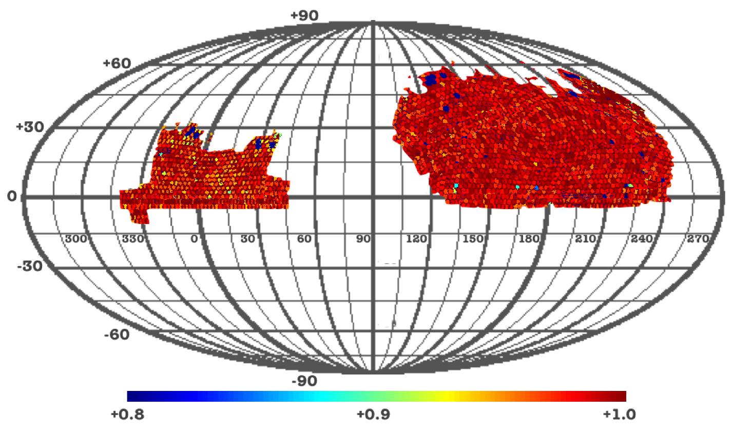
Each spectroscopically observed galaxy is weighted to account for three distinct observational effects: redshift failure, $w_{fail}$; minimum variance, $w_{\rm FKP}$Feldman et al. (1994); and angular variation, $w_{sys}$, which accounts for airmass dependent seeing effects and stellar contamination. These weights are described in more detail in Anderson et al. (2012) and Ross et al. (2012). The total weight for each galaxy is calculated as the product of these weights, i.e., $w_{total}=w_{fail}w_{\rm FKP}w_{sys}$. The random catalog points are also weighted but they only include the minimum variance FKP weight.

The CMASS galaxy sample is distributed over the range $0.43<z<0.7$, with an effective redshift of $z_{\rm eff}=0.57$ and an effective volume of $V_{\rm eff}\sim 6.0\,$Gpc³ calculated as

$$V_{\rm eff}=\sum\left(\frac{{n}(z_{i})P_{0}}{1+{n}(z_{i})P_{0}}\right)^{2}\Delta V(z_{i})\ ,$$ (2)

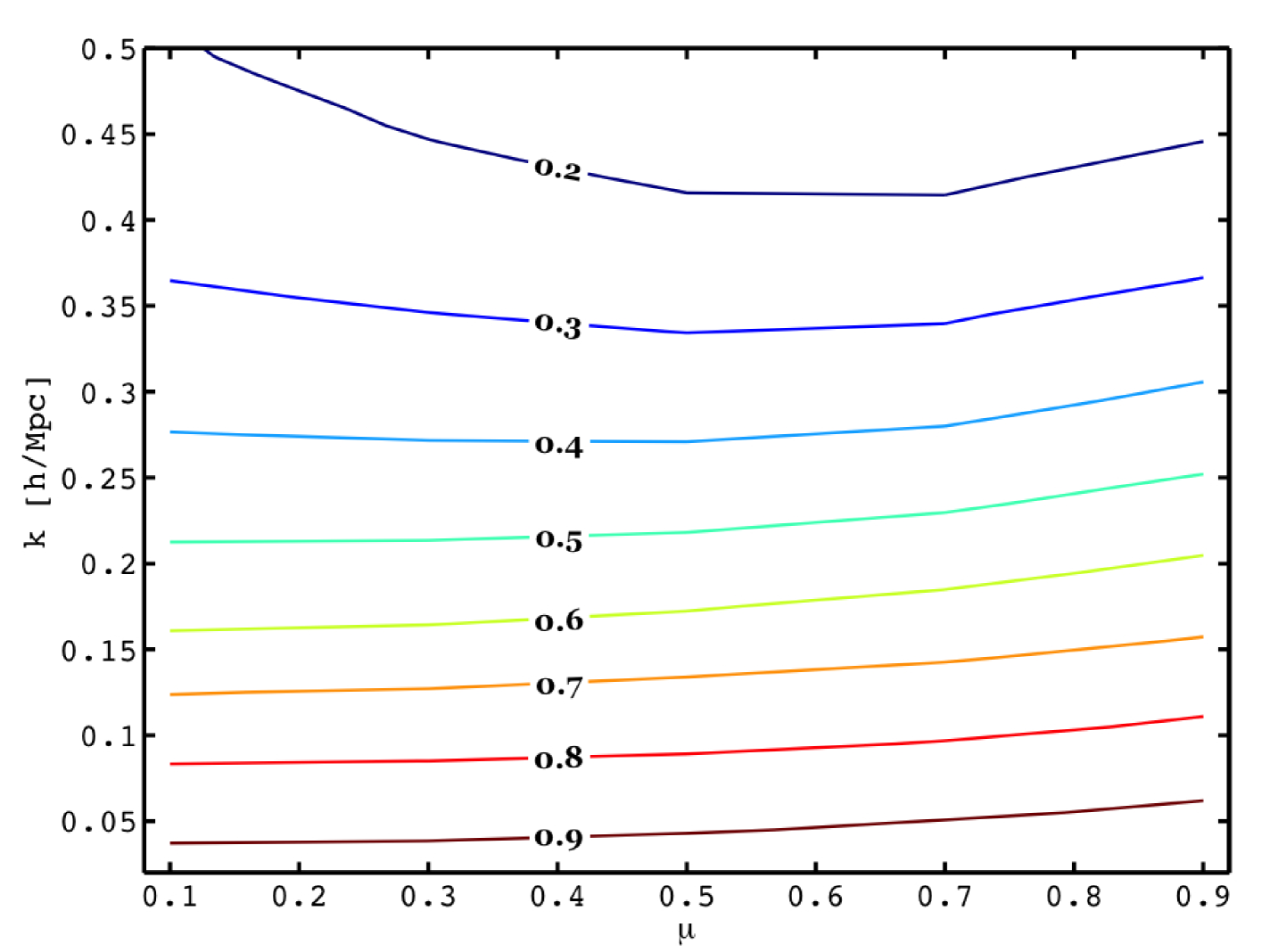
where $\Delta V(z)$ is the volume of a shell at redshift $z$ and $P_{0}=20,000h^{-1}$Mpc. To sample the density and velocity fields more fully, one can either increase the sampling density (raise $nP$) or survey new volumes. Figure 2 shows the sample variance completeness of the DR11 volume for each Fourier mode $k$ and $\mu$, i.e.

$$v(k,\mu)=\left(\frac{\bar{n}P(k,\mu)}{1+\bar{n}P(k,\mu)}\right)^{2}\ ,$$ (3)

where $\bar{n}$ is the average galaxy density within the volume, and the anisotropic power spectrum $P(k,\mu)$ is measured from mock simulations in Okumura et al. (2012). When $v$ approaches unity (for high $nP$) then further information on the density field at that $k$–$\mu$ can only come from surveying different volumes; Fig. 2 can thus be thought of as showing the sample variance completeness.

Figure 2: The normalized effective volume $v(k,\mu)$, showing the sample variance completeness, is plotted. Values near unity mean that new volumes must be surveyed to gain further information on the density and velocity fields; lower values mean further galaxies can contribute information.

We compute the redshift-space 2-dimensional correlation function $\xi(\sigma,\pi)$ of the BOSS DR11 galaxy catalog using the standard Landy-Szalay estimator Landy & Szalay (1993). In the computation of the correlation estimator we use a random point catalogue that constitutes an unclustered but observationally representative sample of the BOSS CMASS survey. The angular points are chosen to reside within the survey geometry with a Monte Carlo acceptance proportional to the RA-Dec sector completeness, and the redshifts are obtained via the random shuffle method of Ross et al. (2012). The randoms are also assigned FKP weights, just as for the galaxies. To reduce the statistical variance of the estimator we use $\sim 50$ times as many randoms as we have galaxies. We perform the coordinate transforms using the fiducial Planck best fit flat $\Lambda$CDM cosmological model ($\omega_{b}=0.022068$, $\omega_{c}=0.12029$, $h=0.67$).

Figure 3: The measured (blue filled contours), best fit (thin black), and LCDM-predicted (thin dotted) cases of $\xi(\sigma,\pi)$ are plotted, using the Planck early universe prior. The thick solid and dashed circles represent 2D BAO rings from the measurement and the Planck LCDM prediction.

We calculate the correlation function in 225 bins spaced by $10\,h^{-1}\,{\rm Mpc}$ in the range $0<\sigma,\pi<150\,h^{-1}\,{\rm Mpc}$. The BOSS sample is naturally separated into North and South samples with 520,805 and 170,021 galaxies respectively, and we measure the anisotropic two-point correlation function in the north, south and combined samples.

Our results depend not only on the correlation functions but also on the errors of these measurements. Also, different bins of the correlation function can be strongly correlated to each other, therefore it is necessary to estimate a covariance matrix to give correct constraints on cosmological parameters.

For this purpose we use PTHALO Manera:2012sc mock galaxy catalogs, updated to reflect the larger observational area. These catalogs were used for BAO analysis in Anderson et al. (2014) and have the same survey geometry and number density as the CMASS galaxy sample that was used in our analysis. The mocks catalogs constitute 600 density field realizations created using second-order Lagrangian perturbation theory (2LPT). The density and velocity fields created using 2LPT eventually break down as one goes to small scales, but it was confirmed by Manera:2012sc ; Reid:2012sw that the correlation functions measured from the mock catalogs based on 2LPT match the one measured from the BOSS survey at scales larger than $20\,h^{-1}\,{\rm Mpc}$. In our analysis below, we will use the data at $s\geq 50\,h^{-1}\,{\rm Mpc}$ and, as we did in Song:2013ejh , to be conservative we will additionally remove the data along the line of sight, which is known to deviate from linear theory starting from larger scales than the data perpendicular to the line of sight (see Sec. IV below). Note that we use these mock catalogs solely to estimate errors of the correlation function measured from the CMASS sample.

For each realization we compute the correlation function as we did for the observed catalog and obtain a covariance matrix as described in detail in Linder:2013lza .

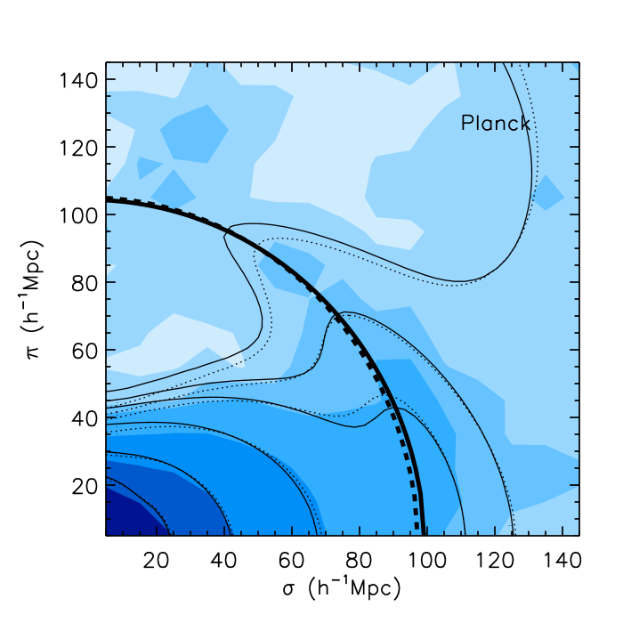
The measured two point correlation function $\xi(\sigma,\pi)$ is presented as blue filled contours in Fig. 3, with the levels of $(0.2,0.06,0.16,0.005,0.002,-0.001,-0.006)$ from the inner to outer contours. The RSD anisotropy is clearly visible, as is the 2D BAO ring at $\sqrt{\sigma^{2}+\pi^{2}}\approx 100~{}\,h^{-1}\,{\rm Mpc}$.

IV Results

IV.1 Cosmology from combined maps

	Planck LCDM	Combined	North	South
$D_{A}$	$936.3$	$954.9^{+19.8}_{-21.6}$	$955.1^{+20.8}_{-21.7}$	$970.4^{+35.8}_{-41.1}$
$H^{-1}$	$2170.8$	$2159.8^{+136.3}_{-117.8}$	$2207.2^{+124.9}_{-103.0}$	$2220.9^{+243.9}_{-358.0}$
$G_{b}$	—	$1.15^{+0.08}_{-0.08}$	$1.10^{+0.07}_{-0.07}$	$1.15^{+0.20}_{-0.19}$
$G_{\Theta}$	$0.46$	$0.41^{+0.09}_{-0.09}$	$0.34^{+0.08}_{-0.08}$	$0.54^{+0.16}_{-0.17}$
$\sigma_{p}$	—	$6.2^{+3.6}_{-3.8}$	$1.5^{+3.3}$	$9.2^{+3.4}_{-4.4}$

Table 2: We present the measured values of $D_{A}\,(\,h^{-1}\,{\rm Mpc})$, $H^{-1}\,(\,h^{-1}\,{\rm Mpc})$, $G_{b}$, $G_{\Theta}$ and $\sigma_{p}\,(\,h\,{\rm Mpc}^{-1})$, and their 68% CL uncertainties, using the combined data, and the north and the south maps separately. Here the cutoffs are $s_{\rm cut}=50\,h\,{\rm Mpc}^{-1}$ and $\sigma_{\rm cut}=40\,h\,{\rm Mpc}^{-1}$.

Information on the late-time cosmological expansion and dynamics are encoded in the distances along and transverse to the line of sight, and the growth of the density and velocity fields. A first consistency check of $D_{A}$ and $H^{-1}$ with the Planck LCDM model can be ascertained by comparing the two 2D BAO rings in Fig. 3. The thick dashed and solid circles represent the rings estimated from the Planck LCDM model and the DR11 measurements. The growth functions do not alter the 2D BAO ring, and it is distorted differently by $D_{A}$ and $H^{-1}$ in the transverse and radial directions. The consistency between the solid and dashed circles means that the measured distances agree well with the Planck LCDM model.

We quantify this in Table 2, where the measured $D_{A}$ and $H^{-1}$ are within the 68% confidence limit of the Planck LCDM prediction. We discuss the effect of $\sigma_{\rm cut}$ below, and of North vs South maps in the next section.

Figure 4: The measured values of $D_{A}$, $H^{-1}$ and $G_{\Theta}$ are shown for various $\sigma_{\rm cut}$ from $30\,h\,{\rm Mpc}^{-1}$ and $60\,h\,{\rm Mpc}^{-1}$. The values have converged for $\sigma_{\rm cut}\geq 40\,h\,{\rm Mpc}^{-1}$, but inclusion of smaller scales biases the answers by $\sim 1\sigma$. The dotted lines, representing the Planck LCDM predictions, are shown purely for reference; the important aspect is convergence (not to any particular value).

For the density and velocity growth factors the information comes from multiple scales, and especially from the redshift space anisotropy. While the signal–to–noise of the inner (higher amplitude) contours of clustering is higher, the use of RegPT to second order is insufficient for accurate modelling of $\xi(\sigma,\pi)$ at scales $s<50\,h\,{\rm Mpc}^{-1}$. In particular, the cross–spectrum between $\delta$ and $\Theta$ is not perfectly cross–correlated. When the cut–off $s<50\,h\,{\rm Mpc}^{-1}$ is applied, the constraints on $G_{b}$ and $G_{\Theta}$ from their distinctive amplification of the inner contours Song:2010kq become weaker, but more robust as we now see.

At small scales, if the non–perturbative effect of FoG is underestimated, then the residual squeezing can be misinterpreted as a smaller $G_{\Theta}$. We expect the FoG effect to be increasingly important at smaller scales, and so these run increasing risk of misestimation. To test this, in Fig. 4 we show the cosmology results as we vary $\sigma_{\rm cut}$ from $30\,h\,{\rm Mpc}^{-1}$ to $60\,h\,{\rm Mpc}^{-1}$. The strongest effect is on $G_{\Theta}$, and indeed inclusion of small scales noticeably lowers the measured $G_{\Theta}$. However, for all $\sigma_{\rm cut}\geq 40\,h\,{\rm Mpc}^{-1}$ the results have converged and the measured values are insensitive to the exact value of $\sigma_{\rm cut}$. This indicates that the approximation for treating FoG should not be trusted for $\sigma<40\,h\,{\rm Mpc}^{-1}$, while above this scale our approach is robust. This argument holds as well for $D_{A}$ and $H^{-1}$, though less extremely. Considerable caution should be applied to the use of the clustering data on small scales.

Figure 5: The 2D joint likelihood contours at 68% and 95% CL measured for $D_{A}$, $H^{-1}$, $G_{b}$ and $G_{\Theta}$ are shown, using $s_{\rm cut}=50\,h\,{\rm Mpc}^{-1}$ and $\sigma_{\rm cut}=40\,h\,{\rm Mpc}^{-1}$. The fiducial values in the Planck LCDM concordance model are shown by x’s (see Table 2).

The outer contours provide another indicative behavior for $G_{\Theta}$. When $G_{\Theta}$ varies, the location of peaks on 2D BAO circle moves differently from the variation of $G_{b}$ Song:2013ejh . The peak points run away from the pivot point (roughly where $\sigma\approx\pi$) as $G_{\Theta}$ decreases, and move toward it for increasing $G_{\Theta}$. From Fig. 3 we see that around the BAO ring the fourth and sixth contours recede away from the Planck LCDM prediction, while the fifth contour, which lies close to the pivot point, has not moved. This implies the measured $G_{\Theta}$ is smaller than the Planck LCDM prediction and indeed we find $G_{\Theta}=0.41\pm 0.09$ in comparison with 0.46 predicted by Planck LCDM prediction. This is still within 68% CL however (note though that using a lower $\sigma_{\rm cut}$ moves $G_{\Theta}$ to even smaller values).

The quantity $G_{b}$ represents the combination of density field and linear bias. As no cosmological model is assumed, the two are not separable. As shown in Table 2, $G_{b}$ is measured to be $1.15\pm 0.08$. If the Planck LCDM model is true, then the linear bias at $z=0.57$ can be estimated to be $b=2.0$ with 7% fractional error (recall that $G_{b}=bD$). This is consistent with what we observe from the simulation.

The velocity dispersion parameter $\sigma_{p}$ for FoG is measured to be $6.2^{+3.6}_{-3.3}\,h^{-1}\,{\rm Mpc}$. The FoG effect is at first order degenerate with $G_{\Theta}$; this causes weak constraints on both $\sigma_{p}$ and $G_{\Theta}$.

IV.2 Testing the cosmological framework

Our model independent analysis allows several consistency tests.

1. In a Friedmann-Robertson-Walker (FRW) cosmology, $D_{A}$ is formed from an integral over $H^{-1}$.

2. Within general relativity and FRW, the growth rate $G_{\Theta}$ and expansion rate $H^{-1}$ are tied together.

3. Neutrino mass suppresses growth, so a measured consistency with Planck LCDM (i.e. minimal neutrino mass) disfavors higher neutrino mass (or requires a conspiracy with enhanced growth from modified gravity – but this would show up in the previous consistency test).

We therefore study the joint probability distribution between the measured cosmological quantities, e.g. the two dimensional likelihood contours of $G_{\Theta}$ vs $H^{-1}$. All such contours are marginalized over the remaining quantities.

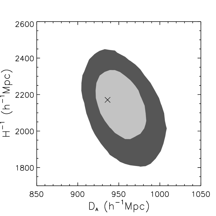
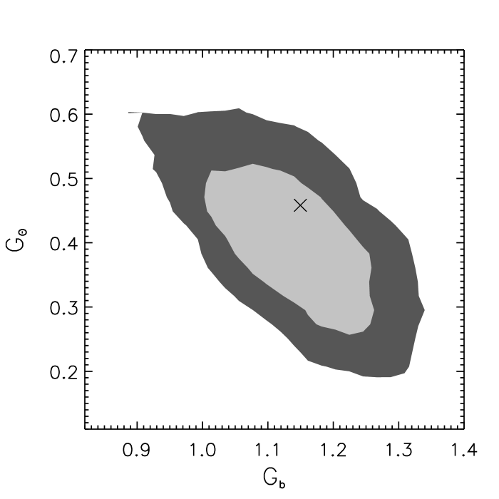
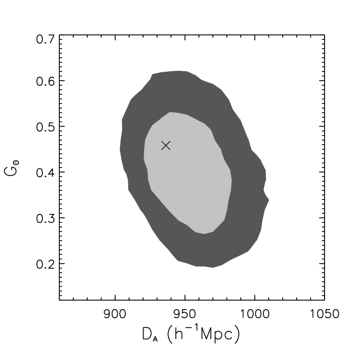
In Fig. 5 we present two dimensional cosmological parameter contours in four different combinations. The x’s represent the best values of Planck LCDM models; we see that our model independent analysis agrees within the 68% confidence level with the cosmology that assumed LCDM, general relativity, and minimal neutrino mass. This holds for all the measured distances and growth functions.

The first panel provides evidence for the FRW consistency relation of the background quantities of the distance and expansion rate. The second panel involves measurements of the perturbed quantities, from the density and velocity fields. As mentioned, $G_{b}$ is consistent with expectations for galaxy bias. The measured $G_{\Theta}$ can be converted to $f\sigma_{8}=0.43\pm 0.09$, with the Planck LCDM model predicting $f\sigma_{8}=0.48$, again within 68% CL. (Note this would not hold if we naively included smaller scales where nonlinear modelling is not robust.)

The third and fourth panels, showing that the joint likelihoods for the background and growth quantities are consistent with Planck LCDM, can be thought of as a (weak, model independent) test of the general relativity criterion. That the fourth panel, showing the $G_{\Theta}$–$H^{-1}$ likelihood, is consistent with Planck LCDM (with minimal neutrino mass), also disfavors a larger neutrino mass and its accompanying suppression of growth. If one assumed that the background cosmology is truly the Planck LCDM model, then the growth measurement could be converted to an estimate of the gravitational growth index $\gamma$ Linder (2005) or a sum of neutrino masses $\sum m_{\nu}$. However for both of these the uncertainty on $G_{\Theta}$ is multiplied by a large prefactor so the constraints are weak.

IV.3 Comparison of North vs South

Figure 6: The measured $D_{A}$, $H^{-1}$ and $G_{\Theta}$ are presented from the top to the bottom panels. Each one shows the results from the combined, northern, and southern skies, from left to right. The dotted lines represent the Planck LCDM predictions.

Another interesting check involves a comparison of the estimated cosmological quantities using only the northern or southern hemisphere sky. The median RA and Dec of each patch is $(185,25)$ and $(2,10)$ respectively (see Fig. 1), so the centers of these two disjoint sky patches are separated by 145 degrees on the sky. The effective volume of the North is 4.5 Gpc³ and that of the South is 1.5 Gpc³.

Table 2 breaks down the cosmological results by hemisphere. All quantities are consistent within 68% CL; nevertheless, there are some interesting patterns worthwhile keeping an eye on as the data improves and the error bars shrink.

In the top and middle panels of Fig. 6 we present the measured $D_{A}$ and $H^{-1}$ for North and South separately, and the full survey combination. North and South agree with each other and with Planck LCDM predictions. The detailed numbers are shown in Table 2. Note that the median measured $H^{-1}$ from the combined map does not lie between the North and South measured values; this occurs due to the non-Gaussian probability distribution for the measured $H^{-1}$ in the South – the mode value is 2116 $h^{-1}\,$Mpc.

For the measured coherent motion $G_{\Theta}$ in the bottom panel, the North is somewhat inconsistent ($\sim 1.5\sigma$) with the Planck LCDM prediction. From Table 2, in the North $G_{\Theta}=0.34^{+0.08}_{-0.08}$ and in the South $G_{\Theta}=0.54^{+0.16}_{-0.17}$, while the LCDM fiducial has $G_{\Theta}=0.46$. The central values of North and South are noticeably different, though due to the large uncertainty from the small effective volume in the South this cannot be said to be statistically significant.

One might speculate about North-South anisotropy but this is disfavored due to the consistency of the measured $H^{-1}$ values. We have also checked that $z_{\rm eff}$ is consistent between North and South, at the 0.05% level. Another possibility is inhomogeneity at the perturbation level, for example an anisotropic stress DeFelice:2013bxa ; Gumrukcuoglu:2013nqa . With a quadrupole dependence, this would not have an effect if the North and South areas were 180^∘ apart, but could have a component as they are separated by 145^∘. Also note that the measured velocity dispersion $\sigma_{p}$ is different in North and South, which could support this. Alternately, the covariance between $\sigma_{p}$ and $G_{\Theta}$ is such that high $\sigma_{p}$ can damp the excess velocity growth of high $G_{\Theta}$, so that these (and the low $\sigma_{p}$, low $G_{\Theta}$ case for the North) lie along the degeneracy direction with LCDM.

V Conclusions

We have carried out an analysis within a framework independent of the cosmological model, i.e. the specific energy density components such as dark energy or curvature. This uses the BOSS DR11 dataset that measures galaxy clustering over the largest volume yet surveyed with an effective redshift of $z=0.57$. We measure the angular distance $D_{A}$, expansion rate $H^{-1}$ (from the radial distance information), and velocity growth rate $G_{\Theta}$; all are consistent with the Planck LCDM prediction.

These are multiple, model independent tests of LCDM since the implications of each parameter is different. The measured $D_{A}$ is insensitive to uncertainties from contamination along the line of sight, but can be affected by the assumption of coherent (scale-independent) galaxy bias on the scales used, due to the degeneracy between $D_{A}$ and $G_{b}$. The value of the galaxy bias $b$ we derive is also consistent with other measurements. For accurate measurement of $H^{-1}$, the radial dependence of $\xi(\sigma,\pi)$ should be modelled robustly.

For $G_{\Theta}$, measured coherent motions are degenerate with the FoG effect which is problematic to model. If there is residual contamination from inaccurate modelling of the FoG effect, the coherent motions and hence velocity growth rate $G_{\Theta}$ or $f\sigma_{8}$ are underestimated. Since the theoretical model calibrated from simulations becomes increasingly inaccurate on small scales, we carefully examine the dependence of the results on the small scale cutoff in the measurements used. We find that convergence is achieved for $\sigma_{\rm cut}\geq 40\,\,h\,{\rm Mpc}^{-1}$, with bias arising if smaller scales are included – an important caution. Our measurement corresponds to $f\sigma_{8}=0.43\pm 0.09$, with the Planck LCDM prediction of $f\sigma_{8}=0.48$.

Considering the joint likelihood of these cosmological quantities, we find consistency with the Planck LCDM model at 68% CL. By comparing the quantities to each other, we can make three general consistency tests of the cosmological framework. We check consistency with the FRW framework, with general relativity, and with minimal neutrino mass and find that all are within 68% CL.

Comparing the galaxy measurements from the North and South sky samples separately, we continue to find consistency with Planck LCDM. Here the reduced effective volume makes the error bars larger, but there are slight discrepancies worth testing with future data from larger surveys such as DESI or LSST. For example, the growth rate in the North has $G_{\Theta}=0.34$ ($\sim 1.5\sigma$ from Planck LCDM) while the South has $G_{\Theta}=0.54$ (though again the error bar is so large that these are consistent within 68% CL). One speculative explanation is the presence of anisotropic stress (affecting the perturbations while keeping the background quantities consistent), but covariance between $G_{\Theta}$ and $\sigma_{p}$ (also measured to be different in North and South) is another possibility. Again, upcoming larger sky surveys will be valuable in testing cosmology in different directions.