Toward Using Surrogates to Accelerate Solution of Stochastic Electricity Grid Operations Problems

Abstract

Stochastic unit commitment models typically handle uncertainties in forecast demand by considering a finite number of realizations from a stochastic process model for loads. Accurate evaluations of expectations or higher moments for the quantities of interest require a prohibitively large number of model evaluations. In this paper we propose an alternative approach based on using surrogate models valid over the range of the forecast uncertainty. We consider surrogate models based on Polynomial Chaos expansions, constructed using sparse quadrature methods. Considering expected generation cost, we demonstrate the approach can lead to several orders of magnitude reduction in computational cost relative to using Monte Carlo sampling on the original model, for a given target error threshold.

I Introduction

Unit commitment (UC) is the fundamental process of scheduling thermal generating units in advance of operations in the electric power grid [1]. The objective is to minimize overall production costs to satisfy forecasted demand for electricity, while respecting constraints on both transmission (e.g., thermal limits) and generator infrastructure (e.g., ramping limits). Economic dispatch (ED) is a closely related operations problem, in which cost minimization is performed to identify an optimal set of power output levels for a fixed set of active thermal generating units. UC and ED are respectively formulated as a mixed-integer and linear optimization problems, and solved using commercial solvers. Despite improvements in forecasting technology, next-day demand predictions are imperfect, with errors on average in the 1-3% range and exceeding 10% on specific days [2]. To account for such inaccuracies, reserve margins are universally imposed in UC. These margins implicitly deal with uncertainty in load forecasts, by ensuring there is sufficient generation capacity available to meet unexpectedly high demand during operations.

An alternative approach to dealing with forecast errors in UC is to explicitly model the load uncertainty, typically via a finite set of sampled realizations from a stochastic process model of load. This approach results in a stochastic UC model (SUC), in which the objective typically is to minimize the expected cost across the load scenarios [3, 4]. By explicitly representing the inherent uncertainty in load forecasts, a SUC solution ensures sufficient flexibility to meet a range of potential load realizations during next-day operations. Further, by explicitly representing uncertainty, reliance on reserve margins is reduced, yielding less costly solutions than those obtained for the deterministic UC problems. While not considered here, we note that the problems induced by increasing rates of renewables (e.g., wind and solar) generation penetration accentuates the differences between stochastic and deterministic UC problems, due to increased errors in the next-day forecasts relative to load. While conceptually appealing, the computational difficulty of stochastic UC is well-known [5], such that it is not presently used in practice. The difficulty is primarily driven by the number of forecast samples required to achieve high-quality, robust solutions.

Uncertainties such as those found in stochastic UC are ubiquitous in both power systems operations and planning, and the importance of credibly accounting for them is well-recognized. However, the lack of advanced methods to handle uncertainty and the limitations of scenario-based approaches have led researchers to seek alternatives. For example, Thiam and DeMarco [6] argue: “Simply put, when uncertainty is credibly accounted for such methods yield solutions for economic benefit of a transmission expansion in which the “error bars” are often larger than the nominal predicted benefit.” Instead, Thiam and DeMarco [6] propose an “oblivious approach” to transmission expansion that does not take into account the uncertainties in the inputs. We agree that an oblivious approach is more credible than simply ignoring large error bars in estimations. However, we posit that with proper modeling and sampling algorithms, the errors incurred in such analyses can be drastically reduced. Of course, it is not possible to change the nature of uncertainties, such that if uncertainties are so large that they fail to provide significant information, oblivious approaches may be appropriate. However, as we argue in this paper, it is possible to reduce additional uncertainties and inefficiencies introduced due to poor modeling and sampling.

In this paper, we propose to adopt advanced modeling and sampling techniques from the uncertainty quantification (UQ) community, and leverage them to impact power systems operations problems such as stochastic UC and ED. Such techniques have been successfully applied in many areas of computational science and engineering, with great success [7]. Most studies analyzing uncertain power system operations problems generate forecast scenarios by drawing random samples from a stochastic process using standard Monte Carlo (MC) techniques. In this paper, we consider instead an alternative approach based on using Polynomial Chaos [8] expansions, built using sparse quadrature methods, as surrogate models valid over the range of the forecast uncertainty. We demonstrate that our approach yields a one to two order of magnitude reduction in the number of samples required to estimate expected generation cost, relative to MC, for a given target error threshold. Consequently, our approach has the potential to dramatically drop the computational difficulty of stochastic UC and ED, significantly reducing the barriers to its use in practice.

The remainder of this paper is organized as follows. We briefly introduce our stochastic UC and ED formulations in Section II, to provide context for our research. In Section III, we detail our surrogate models of load for stochastic UC / ED, based on Polynomial Chaos expansion. We then empirically analyze the accuracy of our surrogates on standard IEEE test problems in Section IV, and conclude in Section V.

II Stochastic Commitment and Dispatch

We now describe a generic formulation of the stochastic UC problem. Our formulation is based on the deterministic mixed-integer linear UC formulation introduced by [1]. Let $G$ and $T$ denote the index sets of thermal generating units and time periods, respectively. We abstractly define the set of unit commitment constraints (i.e., operational and physical constraints on physical units) as $\mathcal{X}$ and let $\bm{x}$ denote the vector of unit commitment decisions. The stochastic UC problem is then given as follows:

$$\min_{\bm{x}}\quad c^{u}(\bm{x})+c^{d}(\bm{x})+\overline{Q}(\bm{x})$$ (1a)

s.t. $$\bm{x}\in\mathcal{X},$$ (1b)

$$\bm{x}\in\{0,1\}^{|G|\times|T|}$$ (1c)

The objective terms $c^{u}(\bm{x})$ and $c^{d}(\bm{x})$ represent generating unit start-up and shut-down costs, respectively, and $\overline{Q}(\bm{x})$ denotes the expected generation cost. The UC constraints prescribed by $\mathcal{X}$ include minimum on-off requirements and linearization of startup and shutdown costs.

We treat the loads $D^{t}$ for all $t\in T$ as random variables (RVs). We begin by setting up a requisite theoretical framework as follows. Define the probability space $(\Omega,\mathfrak{S},P)$, where $\Omega$ is a sample space, $\mathfrak{S}$ is a $\sigma$-algebra on $\Omega$, and $P$ is a probability measure on $(\Omega,\mathfrak{S})$. Further, defining the germ ${\bm{\xi}}=\{\xi_{1},\xi_{2},\ldots,\xi_{|T|}\}$ as a set of independent identically distributed (iid) RVs in $L_{2}(\Omega,\mathfrak{S},P)$, to be further specified below, we focus on the probability space $(\Omega,\mathfrak{S}_{\bm{\xi}},P)$ employing the sigma algebra generated by ${\bm{\xi}}$. We define the uncertain loads as RVs $D^{t}(\omega):\Omega\rightarrow\mathbb{R}$ in $L_{2}(\Omega,\mathfrak{S}_{\bm{\xi}},P)$, such that we may write, by construction, $D^{t}:=D^{t}({\bm{\xi}}(\omega))$, $\forall t\in T$.

Given the uncertain loads expressed as RVs, the corresponding generation cost $Q({\bm{x}},{\bm{\xi}}(\omega))$ is similarly uncertain/random. The expected generation cost, denoted $\overline{Q}(\bm{x})$, is defined as

$$\overline{Q}(\bm{x})=\mathrm{E}_{\bm{\xi}}Q(\bm{x},{\bm{\xi}}(\omega))$$ (2a)

and the uncertain (multi-period) economic dispatch problem under a fixed unit commitment $\bm{x}$ is given by

$Q(\bm{x},{\bm{\xi}}(\omega))=$

$$\min_{\bm{p,q}}\quad \sum_{t\in T}\sum_{g\in G}c_{g}^{P}(p_{g}^{t})+\sum_{t\in T}Mq^{t}$$ (3a)

s.t. $$\sum_{g\in G}p_{g}^{t}-q^{t}=D^{t}(\xi_{t}(\omega)),\quad\forall t\in T$$ (3b)

$$\underline{P}_{g}x_{g}^{t}\leq p_{g}^{t}\leq\overline{P}_{g}x_{g}^{t},\quad\forall g\in G,t\in T$$ (3c)

$$p_{g}^{t}-p_{g}^{t-1}\leq RU(x_{g}^{t-1},x_{g}^{t}),\quad\forall g\in G,t\in T$$ (3d)

$$p_{g}^{t-1}-p_{g}^{t}\leq RD(x_{g}^{t-1},x_{g}^{t}),\quad\forall g\in G,t\in T.$$ (3e)

where

$$RU(x_{g}^{t-1},x_{g}^{t})=R_{g}^{u}x_{g}^{t-1}+{S}_{g}^{u}(x_{g}^{t}-x_{g}^{t-1})+\overline{P}_{g}(1-x_{g}^{t})$$

$$RD(x_{g}^{t-1},x_{g}^{t})=R_{g}^{d}x_{g}^{t}+S_{g}^{d}(x_{g}^{t-1}-x_{g}^{t})+\overline{P}_{g}(1-x_{g}^{t-1})$$

and $R_{g}^{u}/R_{g}^{d}$, $S_{g}^{u}/S_{g}^{d}$ represent nominal ramp-up/ramp-down rates, startup/shutdown ramp rates, respectively.

Note that because the loads are RVs, all solution variables are necessarily RVs. For brevity of notation, we have only included the explicit dependence on ${\bm{\xi}}(\omega)$ in $D^{t}$ and $Q$, thereby emphasizing the randomness of inputs/output of interest only.

The optimization objective in stochastic ED is to minimize the expected total production and loss-of-load costs. The first term in (3a) represents total production cost. The second term represents the loss-of-load penalty, where $q^{t}$ is the unit (e.g., MW) of load unsatisfied in period $t$. Typically, the load-shedding penalty is equal to a large number $M$. Constraints (3b)-(3e) specify operational constraints, and include (in order): power balance at each period (3b); lower and upper bounds for committed generation unit output levels (3c); and generation ramp-up and ramp-down constraints for pairs of consecutive time periods (3d) and (3e).

A quadratic production cost function, given below, is typically employed in scheduling electricity grid operations.

$$c^{P}_{g}(p_{g}^{t})=a_{g}x_{g}^{t}+b_{g}p_{g}^{t}+c_{g}(p_{g}^{t})^{2}$$ (4)

Equation (4) can be accurately approximated by a set of piecewise linear segments. For conciseness, we omit these standard linearization steps. For a detailed treatment on the linearization of the quadratic cost function please refer to [1].

The stochastic ED problem is embedded as a sub-problem in the stochastic UC problem. The high-level context in stochastic UC is the presence of uncertainty in future loads (and, more generally, renewables and system component failures). In stochastic UC, the first-stage decisions are the unit commitment selections $\bm{x}$, and the objective is to minimize the expected generation costs. In the second (recourse) decision stage, uncertain loads result in uncertain recourse decisions for the dispatch variables $\bm{p}$ and $\bm{q}$, and associated generation and load shedding costs. First-stage unit commitment decisions are determined by taking their future impacts into consideration. These future impacts are quantified by the recourse function $\overline{Q}(\bm{x})$, which computes the expected value of generation cost for a given unit commitment $\bm{x}$.

We can estimate the expected generation cost by using a finite number of load realizations (i.e., scenarios) $s\in\mathcal{S}$ sampled from the joint density $p(\bm{D})$, where $\bm{D}=\{D^{1},D^{2},\ldots,D^{|T|}\}$. Defining $\rho\equiv 1/|\mathcal{S}|$, formulation (1) can be rewritten as:

$$\min_{\bm{x}}\quad c^{u}(\bm{x})+c^{d}(\bm{x})+\rho\sum_{s\in\mathcal{S}}Q(\bm{x},s)$$ (5a)

s.t. $$\bm{x}\in\mathcal{X},$$ (5b)

$$\bm{x}\in\{0,1\}^{|G|\times|T|}$$ (5c)

where $Q(\bm{x},s)=$

$$\min_{\bm{p,q}}\quad \sum_{t\in T}\sum_{g\in G}c_{g}^{P}(p_{g}^{t})+\sum_{t\in T}Mq^{t}$$ (6a)

s.t. $$\sum_{g\in G}p_{g}^{t}-q^{t}=D^{t}_{s},\quad\forall t\in T$$ (6b)

$$\underline{P}_{g}x_{g}^{t}\leq p_{g}^{t}\leq\overline{P}_{g}x_{g}^{t},\quad\forall g\in G,t\in T$$ (6c)

$$p_{g}^{t}-p_{g}^{t-1}\leq RU(x_{g}^{t-1},x_{g}^{t}),\quad\forall g\in G,t\in T$$ (6d)

$$p_{g}^{t-1}-p_{g}^{t}\leq RD(x_{g}^{t-1},x_{g}^{t}),\quad\forall g\in G,t\in T.$$ (6e)

Formulation (5) represents an extensive form of the stochastic UC problem, based on $|\mathcal{S}|$ sampled scenarios of load realizations. Formulation (3) can be similarly discretized.

III Accurate estimation with limited samples

The typical scenario sampling approach described above uses Monte Carlo (MC) sampling to approximate an integration, thereby estimating an expectation. While MC algorithms are commonly used for their convenience and robustness, their poor convergence rate is well-known. The MC estimate of the expectation has error

$$\mathrm{V}[Q(\bm{x},{\bm{\xi}})]/\sqrt{|S|},$$ (7)

where $\mathrm{V[Q]}$ denotes the variance of the RV $Q$. Given the significant additional complexity incurred by including stochasticity in the optimization problem, a stochastic formulation becomes advantageous relative to a deterministic formulation when the variance is large. Hence, accurate estimation of the expectation is not only an academic exercise but is important in practice.

According to Eq. (7), accurate estimation can be achieved by increasing the number of samples. However, a linear decrease in error requires a quadratic increase in the number of samples, which can quickly render the stochastic optimization problem intractable. This illustrates the limitation of MC algorithms in providing accurate estimations; while they are convenient, they are not efficient.

Similar problems arise in uncertainty quantification (UQ) for computational science in general, where each sample point typically corresponds to a full simulation. Here, estimation accuracy is of paramount importance, as simulation results may lead to scientific discoveries or high-impact policy decisions. The need for accurate estimation of uncertain model outputs, along with the prohibitive cost of MC samples, have lead to the development of efficient alternatives to MC methods in UQ. In this paper, we illustrate how we adopt such methods for stochastic optimization problems in power systems. The details of the proposed method will be explained subsequently. The key utility of the proposed approach is that it enables, in a preprocessing step, efficient construction of a compact, accurate, and computationally inexpensive representation of the input-output map of the uncertain system. This representation is then used as a surrogate for the dependence of select model-output quantities of interest (QoIs) on uncertain model inputs. Using this surrogate, rather than the original system governing equations, enables accurate estimation of uncertain QoIs, and associated expectations, with minimal costs beyond those of surrogate construction.

III-A Representation of uncertainty using Polynomial Chaos

Given the formulation in Eq. (3) with uncertain/random loads leading to uncertain/random generation costs, we employ efficient UQ methods that rely on functional representations of random variables. Specifically, we use Polynomial Chaos (PC) expansions. A brief description of PC is presented below. For an in-depth description, the reader is referred to a series of publications on this topic [9, 8, 10, 11].

Considering the above defined germ ${\bm{\xi}}$ and the associated probability space $(\Omega,\mathfrak{S}_{\bm{\xi}},P)$, any RV $X:\Omega\rightarrow\mathbb{R}$, where by construction $X\in L_{2}(\Omega,\mathfrak{S}_{\bm{\xi}},P)$, can be written as a PC expansion (PCE):

$$X(\omega)=X({\bm{\xi}}(\omega))=\sum_{k=0}^{\infty}\alpha_{k}\Psi_{k}({\bm{\xi}})$$ (8)

where the basis functions $\Psi_{k}$ are multivariate polynomials that are orthogonal, by construction, with respect to the density of ${\bm{\xi}}$. Thus

$$\langle\Psi_{i}\Psi_{j}\rangle=\int\Psi_{i}(\xi)\Psi_{j}(\xi)dP(\xi)=\delta_{ij}\langle\Psi_{i}^{2}\rangle$$ (9)

where $\delta_{ij}$ is Kronecker’s delta. Further, given this orthogonality, we have

$$\alpha_{k}=\frac{\langle X\Psi_{k}\rangle}{\langle\Psi_{k}^{2}\rangle}$$ (10)

where the inner product is defined, for any RV $Z({\bm{\xi}})$, by the Galerkin projection

$$\langle Z\rangle=\int Z({\bm{\xi}})p_{\bm{\xi}}({\bm{\xi}})d{\bm{\xi}}.$$ (11)

Moreover, the $\Psi_{k}$ are products of univariate polynomials, namely $\Psi_{k}({\bm{\xi}})=\psi_{k_{1}}(\xi_{1})\cdots\psi_{k_{n}}(\xi_{n})$, where $n=|T|$. In a practical computational context, one truncates the PCE to order $p$. The number of terms in the resulting finite PCE

$$X\approx\sum_{k=0}^{P}\alpha_{k}\Psi_{k}({\bm{\xi}})$$ (12)

is given by $P+1={(n+p)!}/{n!p!}$. We dispense with the $\approx$ symbol in the remainder of this paper, employing for any RV $X({\bm{\xi}})$ its truncated PCE

$$X=\sum_{k=0}^{P}\alpha_{k}\Psi_{k}({\bm{\xi}}).$$ (13)

Generalized PC (gPC) expansions have been developed by [11] using a broad class of orthogonal polynomials in the ”Askey” scheme [12]. Each family of polynomials corresponds to a given choice of distribution for the $\xi_{i}$ and is, by construction, orthogonal with respect to the density of $\xi_{i}$. In general, the most useful choices for $({\bm{\xi}},\Psi)$ are uniform RVs with Legendre polynomials and normal RVs with Hermite polynomials.

III-B Surrogate Construction

We employ Legendre-Uniform (LU) PC, as it is most useful for purposes of surrogate construction. Further, in this particular context, i.e., explicitly for surrogate construction, a key first step is to define the input random variables as iid uniform over their ranges of interest. This does not restrict the utility of the approach to iid uniform load distributions. Rather, the uniform assumption is simply to ensure uniform accuracy in the surrogate over the range of loads variability. Once the surrogate is available, providing effectively the input-output map, any $p(\bm{D})$ can be employed, as is further outlined below.

Since, by construction, for LU PC, $\xi_{t}\stackrel{{\scriptstyle iid}}{{\sim}}U(-1,1),\ \forall t\in T$, defining $D^{t}\stackrel{{\scriptstyle iid}}{{\sim}}U(D^{t}_{\mathrm{min}},D^{t}_{\mathrm{max}})$, we have the PCE for $D^{t}$ given simply by

$$D^{t}=\xi_{t}\frac{D^{t}_{\mathrm{max}}-D^{t}_{\mathrm{min}}}{2}+\frac{D^{t}_{\mathrm{max}}+D^{t}_{\mathrm{min}}}{2},\quad\forall t\in T.$$ (14)

In this context we employ Eq. (13) to represent $Q(\bm{x},{\bm{\xi}})$ with a truncated LU PCE

$$Q_{\mathrm{PC}}(\bm{x},{\bm{\xi}})=\sum_{k=0}^{P}c_{k}(\bm{x})\Psi_{k}({\bm{\xi}}),$$ (15)

where $\Psi_{k}({\bm{\xi}})$ are $n$-variate Legendre polynomials ($n=|T|$). The coefficients $c_{k}$ depend on the discrete variable $\bm{x}$, hence separate PCE approximations for $Q$ will be constructed for each instance of $\bm{x}$. Given Eq. (11), we have

$$c_{k}(\bm{x})=\frac{\langle Q\Psi_{k}\rangle}{\langle\Psi_{k}^{2}\rangle}=\frac{1}{\langle\Psi_{k}^{2}\rangle}\int_{[-1,1]^{n}}Q(\bm{x},{\bm{\xi}})\Psi_{k}({\bm{\xi}})d{\bm{\xi}}.$$ (16)

where we have used $p_{\bm{\xi}}({\bm{\xi}})=1$, for ${\bm{\xi}}\in[-1,1]^{n}$.

Given $Q_{\mathrm{PC}}(\bm{x},{\bm{\xi}})$, then for the given $D^{t}\stackrel{{\scriptstyle iid}}{{\sim}}U(D^{t}_{\mathrm{min}},D^{t}_{\mathrm{max}})$, $\forall t\in T$, we have immediately that

$${\overline{Q}}(\bm{x})=\mathrm{E}_{\bm{\xi}}[Q(\bm{x},{\bm{\xi}})]=\langle Q(\bm{x},{\bm{\xi}})\rangle=c_{0},$$ (17)

being the solution of the stochastic ED problem, as required for the stochastic UC problem specified in Eq. (1).

Beyond this, however, the PCE $Q_{\mathrm{PC}}(\bm{x},{\bm{\xi}})$ can be used as a surrogate for the ED problem solution $Q(\bm{x},{\bm{\xi}})$. Specifically, $Q_{\mathrm{PC}}(\bm{x},{\bm{\xi}}(\bm{D}_{s}))\approx Q(\bm{x},s)$ (see Eq. 6) for any demand $\bm{D}_{s}\in\mathbb{D}$ where $\mathbb{D}=\{\bm{D}|D^{t}\in[D^{t}_{\mathrm{min}},D^{t}_{\mathrm{max}}]\,\forall t\in T\}$, employing

$$\xi_{t}=\frac{2D^{t}-(D^{t}_{\mathrm{max}}+D^{t}_{\mathrm{min}})}{D^{t}_{\mathrm{max}}-D^{t}_{\mathrm{min}}},\quad\forall t\in T.$$ (18)

Thus, for any arbitrary $p(\bm{D})$, the PCE $Q_{\mathrm{PC}}(\bm{x},{\bm{\xi}}(\bm{D}))$ can be used to efficiently provide samples $Q(\bm{x},s)$ given random samples ${\bm{D}}_{s}\sim p(\bm{D})$, as long as ${\bm{D}}_{s}\in\mathbb{D}$. Thus, the MC estimation of the expectation $\overline{Q}=\rho^{-1}\sum_{s\in\mathcal{S}}Q(\bm{x},s)$ in Eq. (5a) can be done with arbitrarily large $|\mathcal{S}|$ given the low cost of samples. Alternatively, for any $p(\bm{D})$, one can employ the PCE for $\bm{D}({\bm{\eta}})$, where ${\bm{\eta}}$ is suitable PC germ, and use sparse-quadrature methods outlined below to evaluate projection integrals – but now using as forward model the surrogate $Q_{\mathrm{PC}}(\bm{x},{\bm{\xi}}(\bm{D}({\bm{\eta}})))$, to arrive at the PCE for $Q(\bm{x},{\bm{\eta}})$, from which one easily has $\overline{Q}\equiv c_{0}$, as long as the sparse-quadrature samples $\bm{D}({\bm{\eta}}_{q})\in\mathbb{D}$. The only remaining issue is the evaluation of the projection integrals in Eq. (16), which we discuss below.

III-C Evaluation of the Projection Integrals

Several methods can be employed to evaluate the projection integrals in Eq. (16). MC methods can be used in principle, but are impractical given their slow convergence rate. Alternatively, for smooth integrands, and particularly in low-moderate dimensional problems, sparse quadrature methods [13, 14, 15] can provide highly accurate results with smaller numbers of deterministic samples.

Figure 1: Placement of deterministic samples via a sparse grid approach.

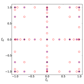
Figure 1 shows the locations of deterministic samples we use, with a sparse grid employing Clenshaw-Curtis quadraure. Several nested levels are shown in the figure, with “+”, “x”, and “o” markers to illustrate the fact that model evaluations can be re-used if higher-order approximations are necessary. The number of requisite samples using sparse-quadrature evaluation of the projection integrals, for a given requisite surrogate accuracy, is much smaller than the corresponding number of MC samples, as we now illustrate.

IV Numerical Results

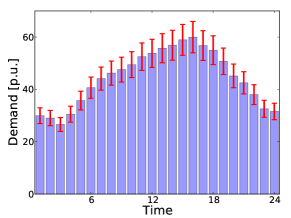
We now present numerical results comparing the calculation of the expected cost of ED via our proposed surrogate model with the classical approach via Monte Carlo scenario sampling. We consider two cases: a 9-bus example [16] and the IEEE 118-bus test system [17]. We vary the number of time periods $|T|$ from 6 to 24. Following the model and analysis in [1], we relax transmission constraints and focus on generating unit characteristics. In Figure 2, we show a typical load series for the IEEE 118 bus test system. The red bars depict a $20\%$ uncertainty range around the nominal values.

Figure 2: Uncertain demand values for the IEEE 118-bus example. The error range is 20% around the nomical values.

We first proceed to test the accuracy of the PCE surrogate for $Q(\bm{x},\bm{\xi}(\bm{D}))$ with respect to full model evaluation. For this exercise we select the 9-bus model since the full model evaluation is expensive, hence we can fully explore the high-dimensional demand space. Table I shows the relative $L_{2}$ error computed with the discrepancies observed at quadrature points between truncated PCEs, in Eq. (15), and the cost values via direct evaluations. Several sparse quadrature levels are employed. The table shows results for PCE orders from $1$ through $4$. A three-level sparse quadrature, denoted L3 in the table, is sufficient to construct a second-order PCE model with a negligible error compared to the full model. Moreover, depending on the purpose of the PCE model, a first-order approximation can also be sufficient. Cross-validation tests using ensembles with $10^{6}$ random samples, results not shown, confirm the high accuracy of the PCE model.

Order	Sparse Quadrature
	L2, 85p	L3, 389p	L4, 1457p	L5, 4865p
1	1.62e-05	2.90e-05	2.15e-05	2.18e-05
2	-	7.48e-07	2.17e-07	7.83e-08
3	-	-	1.92e-07	5.36e-08
4	-	-	-	2.10e-08

TABLE I: Relative $L_{2}$ error at training points for several PCE surrogates and sparse quadrature levels. Power generation cost discretized using 10 segments.

Similar tests indicate that point-wise discrepancies between the PCE surrogate and the full model are less than $0.5\%$ throughout the computational domain for a 2nd order PCE.

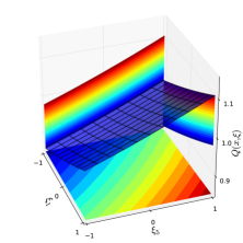
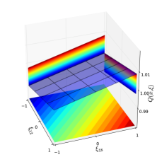
Figure 3 illustrates the dependence of cost on the load in specific time periods. This figure shows 2-dimensional slices through the load spaces for the 9-bus (top frame) and 118-bus (bottom frame) models. The cost $Q$ in these graphics is normalized by the expected value for each case, and $\xi_{t}$ is computed from $D^{t}$ using Eq. (18).

Figure 3: Top frame: Slice through a 6-dimensional 2nd order PCE model for the 9-bus system. Bottom frame: Slice through a 24-dimensional PCE model for the 118-bus system. The transparent surface shows the 3D dependence of $Q$ on the corresponding loads. Filled contours are projected on the side planes to provide a qualitative view of the dependence on each load.

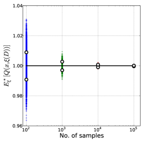
Our research goal in this paper is to demonstrate the efficiency of using PCE to compute (approximate) the expected cost over all possible load realizations. Figure 4 shows the convergence of the standard deviation of the expected cost for the 9-bus model with 6 load periods, evaluated using a number of scenarios between $10^{2}$ and $10^{5}$. These results indicate that about $10^{4}$ samples are necessary to reduce the relative error of the expected cost to below $10^{-3}$.

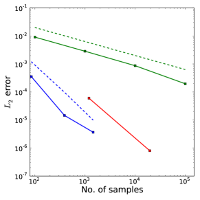
Figure 5 shows sample convergence rates for MC compared to the PCE approach. For MC, a relative error of $10^{-3}$ requires approximately $10^{4}$ model evaluations. The number of model evaluations is independent of the number of loads periods, and is nearly the same for the 9-bus and 118-bus systems. For the surrogate model approach, the number of model evaluations represents the cost of building the PCE. This cost is higly dependent on the dimensionality of the surrogate. For example, the number of model evaluations for a 24-dimensional PCE is one to two orders of magnitude larger compared to a 6-dimensional PCE. Once the PCE is constructed, subsequent evaluations of $\overline{Q}(\bm{x})$ incur negligible cost. Hence the efficiency of the surrogate model approach over the routine MC approach is proportional to the number of times $\overline{Q}$ needs to be evaluated during a simulation. For the 118-bus model, $10^{3}$ evaluations of Eq. (2) results in a computational time about $10^{4}$ times smaller for the PCE approach compared to the traditional MC approach.

V Conclusion

In this paper, we present an approach to reduce the computational cost associated with stochastic unit commitment and economic dispatch, by reducing the number of required forecast samples. This approach is based on surrogate models for the generation cost that cover the uncertainty of forecast load. The surrogate models are constructed using Polynomial Chaos Expansions. The construction of the terms in the surrogate models is based on the projection of the model on increasingly higher basis modes. Consequently, the global error in an $L_{2}$ sense between the surrogate model and the actual simulations is easily controlled.

Figure 4: Convergence of $\overline{Q}(\bm{x})=\mathbb{E}_{\bm{\xi}}Q(\bm{x},\bm{\xi}(\bm{D}))$ computed via MC vs PCE. Scatter plots show normalized $\mathbb{E}_{\bm{\xi}}Q(\bm{x},\bm{\xi}(\bm{D}))$ computed an increasing number of MC samples. The filled circles show $\pm\sigma$ for each ensemble, and the horizontal line shows the values computed via PCE. The expectation values are normalized by the “true” value obtained by MC using $10^{6}$ samples.

We present computational results using 9-bus and 118-bus test cases. For both of these cases, quadratic surrogate models for the generation cost showed global $L_{2}$ errors less than $10^{-4}$ while pointwise errors were less than $1\%$ throughout the uncertain demand space. The construction of Polynomial Chaos surrogate models typically requires a much smaller number of samples, typically one to two orders of magnitude for the examples considered in this paper, compared to Monte Carlo evaluation of the expected generation cost for a given requisite accuracy. Subsequent evaluation of the generation cost statistics via surrogate models incurs negligible additional cost, thereby potentially reducing the computational expense of the forecast ensembles in a stochastic unit commitment and economic dispatch by several orders of magnitude.

Figure 5: Convergence of $\overline{Q}(\bm{x})=\mathbb{E}_{\bm{\xi}}Q(\bm{x},\bm{\xi}(\bm{D}))$ computed via MC (solid green line) vs PCE. The results for a 6-dimensional PCE corresponding to the 9-bus case with 6 load periods is shown with solid blue line, while the results for a 118-bus case with 24 load perionds and the equivalent 24-dimensional PCE is shown with solid red line. The dashed lines show theoretical convergence rates of $1/2$ (green) and $2$ (blue).

References

- [1] M. Carrion and J. Arroyo, “A computationally efficient mixed-integer linear formulation for the thermal unit commitment problem,” IEEE Transactions on Power Systems, vol. 21, no. 3, 2006.
- [2] “ISO New England: Forecast and scheduling reserve adequacy analysis ,” www.iso-ne.com/support/training/courses/wem101/ 10_forecast_scheduling_callan.pdf, accessed: 2014-05-19.
- [3] P. Ruiz, R. Philbrick, E. Zack, K. Cheung, and P. Sauer, “Uncertainty management in the unit commitment problem,” IEEE Transactions on Power Systems, vol. 24, no. 2, pp. 642–651, 2009.
- [4] S. Takriti, J. Birge, and E. Long, “A stochastic model for the unit commitment problem,” IEEE Transactions on Power Systems, vol. 11, no. 3, pp. 1497–1508, 1996.
- [5] A. Papavasiliou, “Coupling renewable energy supply with deferrable demand,” Ph.D. dissertation, University of California Berkeley, 2011.
- [6] F. B. Thiam and C. L. DeMarco, “Optimal transmission expansion via intrinsic properties of power flow conditioning,” in 2010 North American Power Symposium (NAPS), 2010, pp. 1–8.
- [7] H. Najm, “Uncertainty Quantification and Polynomial Chaos Techniques in Computational Fluid Dynamics,” Annual Review of Fluid Mechanics, vol. 41, no. 1, pp. 35–52, 2009.
- [8] R. Ghanem and P. Spanos, Stochastic Finite Elements: A Spectral Approach. Springer Verlag, New York, 1991.
- [9] N. Wiener, “The homogeneous chaos,” Am. J. Math., vol. 60, pp. 897–936, 1938.
- [10] S. Janson, Gaussian Hilbert Spaces. Cambridge, UK: Camb. Univ. Press, 1997.
- [11] D. Xiu and G. Karniadakis, “The Wiener-Askey polynomial chaos for stochastic differential equations,” SIAM Journal on Scientific Computing, vol. 24, no. 2, pp. 619–644, 2002.
- [12] R. Askey and J. Wilson, “Some basic hypergeometric polynomials that generalize jacobi polynomials,” Memoirs Amer. Math. Soc., vol. 319, pp. 1–55, 1985.
- [13] S. A. Smolyak, “Quadrature and interpolation formulas for tensor products of certain classes of functions,” Soviet Mathematics Dokl., vol. 4, pp. 240–243, 1963.
- [14] T. Gerstner and M. Griebel, “Numerical integration using sparse grids,” Numerical Algorithms, vol. 18, pp. 209–232, 1998.
- [15] P. Conrad and Y. Marzouk, “Adaptive smolyak pseudospectral approximations,” SIAM Journal on Scientific Computing, vol. 35, no. 6, pp. A2643–A2670, 2013.
- [16] “Dynamic networks and area aggregation,” in Time-Scale Modeling of Dynamic Networks with Applications to Power Systems, ser. Lecture Notes in Control and Information Sciences, J. H. Chow, Ed. Springer Berlin Heidelberg, 1982, vol. 46, pp. 59–93.
- [17] “Power Systems Test Case Archive ,” http://www.ee.washington.edu/research/pstca/, accessed: 2014-05-01.