The Jones polynomial and Its Limitations
(Master’s Thesis)

Daniel Amankwah
African Institute for mathematical Sciences
Mbour, Senegal
Abstract

This paper will be an exposition of the Kauffman bracket polynomial model of the Jones polynomial, tangle methods for computing the Jones polynomial, and the use of these methods to produce non-trivial links that cannot be detected by the Jones polynomial.

Keywords: Links, Bracket polynomial, Jones polynomial.

This paper is the text of the author’s Master’s Thesis written at the African Institute for mathematical Science under the supervision of Professor Louis H. Kauffman and Dr. Amadou Tall.

1 Introduction

In knot theory, the first polynomial invariant to be discovered was the Alexander polynomial by J.W. Alexander[3]. It was until 198519851985 the New Zealand mathematician, Vaughan Jones announced a new invariant for knots and links called the Jones polynomial[18, 19]. He had noticed some relations in the field of operator theory that appeared similar to relations among knots. The Jones polynomial as an advantage over the Alexander is able to distinguish between a knot or link and it’s mirror image (i.e. detects chirality) and importantly it is able to detect more accurately whether a knot is knotted or a link is linked. A fundamental open problem in knot theory specifically the theory of Jones polynomial is as to whether there exists a non-trivial knot whose Jones polynomial is the same as the unknot. In this project we follow the method in [17] by Shalom Eliahou, Louis H. Kauffman and Morwen B. Thistlethwaite with more detail to construct links whose linking is not detectable by the Jones polynomial.

In section 222, we discuss briefly some elementary definitions and notions in knot theory including some common knots invariants. We give an exposition to the Kauffman bracket model of the Jones polynomial in section 333 and also discuss how the bracket applies to double stranded knots and links. In section 444 we introduce some definitions and notations in tangle theory and apply tangle calculus in proving some relevant propositions associated with our method. We conclude by finally describing the method with an example to illustrate an infinite sequence of a 2-component link whose linking is not detectable by the Jones polynomial and also showing how the Thistlethwaite’s link discovered by Morwen B. Thistlethwaite in [14] fits into our construction.

2 Elementary Terminologies

2.1 Knots and Links

Definition 2.1.

A knot is an isotopy class of an embedding of a circle in 3superscript3\mathbb{R}^{3}. We assume that knots can be given a piecewise linear representation.

Definition 2.2.

An isotopy from a knot or link K𝐾K to Ksuperscript𝐾K^{\prime} is a family of embedding Ktsubscript𝐾𝑡K_{t}, 0t10𝑡10\leq t\leq 1 such that K0=Ksubscript𝐾0𝐾K_{0}=K and K1=Ksubscript𝐾1superscript𝐾K_{1}=K^{\prime}.

Definition 2.3.

Two knots K𝐾K and Ksuperscript𝐾K^{\prime} are equivalent if there exists an orientation preserving homeomorphism, h:33:superscript3superscript3h:\mathbb{R}^{3}\longrightarrow\mathbb{R}^{3} such that h(K)=K𝐾superscript𝐾h(K)=K^{\prime}. Here K,K3𝐾superscript𝐾superscript3K,K^{\prime}\in\mathbb{R}^{3} are embedding of circle into the three-sphere S3superscript𝑆3S^{3}.

It is a fact that two piecewise linear knots are isotopic if and only if they are equivalent. (See [1, 15])

Definition 2.4.

A link is the nonempty union of a finite number of disjoint knots.

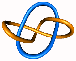
Since the components in a link are disjoint, the knots in a link are the connected components of that link. In particular, a knot is a special case of a link with one component. Some well-known links are shown in Figure  1.
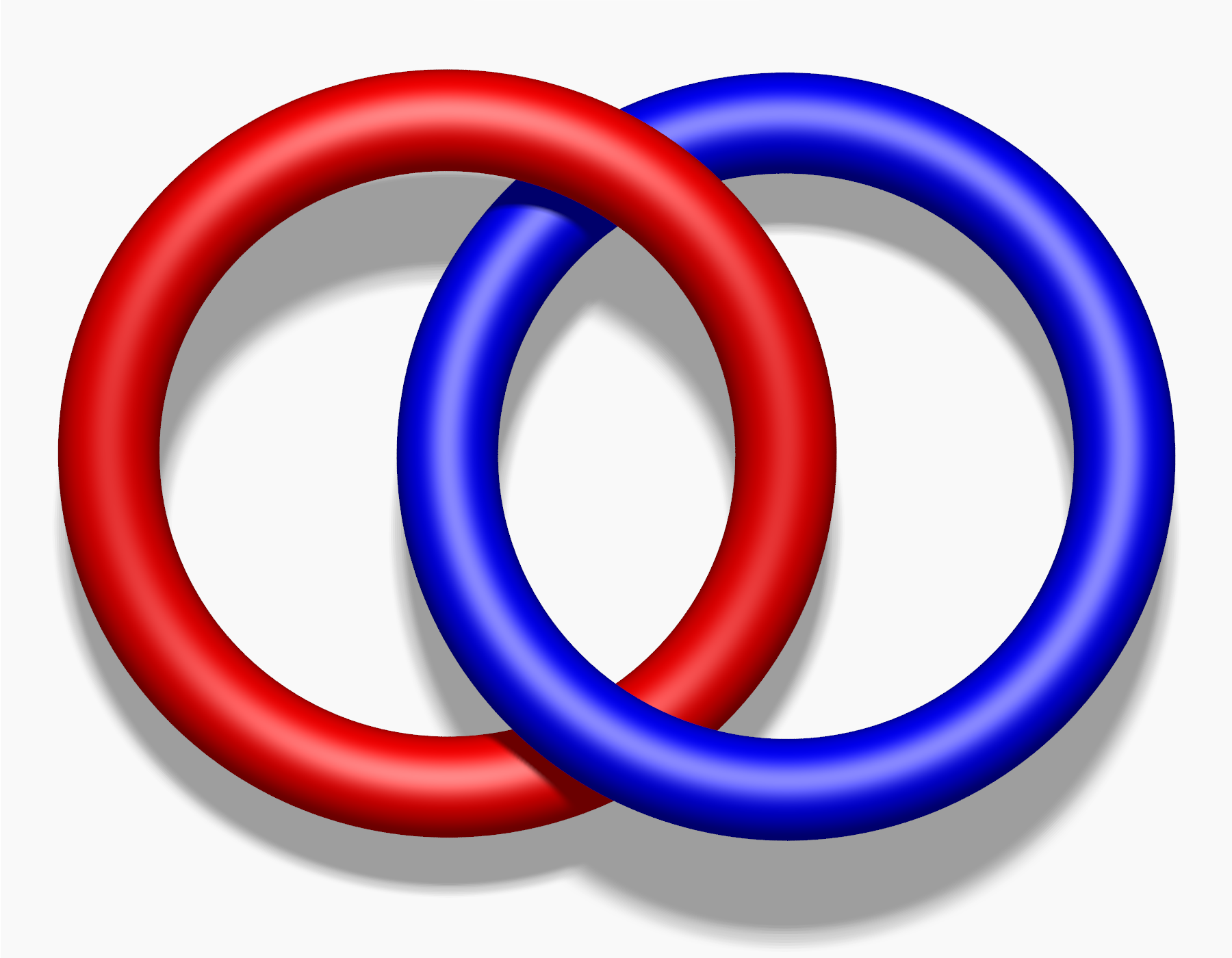
Refer to caption
(a) hopf link
Refer to caption
(b) Borromean rings
Refer to caption
(c) Whitehead link
Figure 1: Examples of link

A useful way to visualize and manipulate a knot is to project it onto a plane.Think of the knot casting a shadow on that plane. A small change in the direction of projection will ensure that it is one-to-one except at the double points, called crossings where the ”shadow” of the knot crosses itself once transversely. At each crossing, to be able to recreate the original knot, the over-strand must be distinguished from the under-strand. This is often done by creating a break in the strand going underneath. The resulting diagram is an immersed plane curve with the additional data of which strand is over and which strand is under at each crossing. These diagrams are called knot diagrams when they represent a knot and link diagrams when they represent a link.

Definition 2.5.

A trivial knot is a knot that is equivalent to a circle in a plane. A trivial link is a link that is equivalent to the union of disjoint circles lying in a plane.

2.2 Reidemeister moves

Definition 2.6.

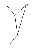
Consider a triangle ABC𝐴𝐵𝐶ABC with side AC𝐴𝐶AC matching one of the line segments of a knot.In the plane determined by the triangle, we require that the region bounded ABC𝐴𝐵𝐶ABC intersects K𝐾K only in the edge AC𝐴𝐶AC. A triangular detour involves replacing the edge AC𝐴𝐶AC of the knot K𝐾K with the two edges AB𝐴𝐵AB and BC𝐵𝐶BC to produce a new knot L𝐿L. With the same notation, a triangle shortcut involves replacing the two edges AB𝐴𝐵AB and BC𝐵𝐶BC of knot L𝐿L with the single edge AC𝐴𝐶AC to produce knot K𝐾K. A triangular move is either a triangular detour or a triangular shortcut.

Refer to caption
(a) K𝐾K
Refer to caption
(b) A triangle on a line segment of the knot K𝐾K
Refer to caption
(c) L𝐿L
Figure 2: A triangular detour on K𝐾K; a triangular shortcut on knot L𝐿L

Although a triangular move is a simple enough step in transforming one knot into an equivalent knot, such a change in a knot can significantly alter the diagram of the knot. We would like to consider triangular moves that only affect the knot diagram one vertex or one edge at a time. This enables us to analyze the effect of the move on some quantity we are trying to establish as a knot invariant.

In the 1920s Kurt Reidemester realized that the triangular moves can be broken down so the effect on the knot diagram is one of three simple modifications or their inverses. We designate the Reidemeister moves as Type I𝐼I(add or remove a curl), Type II𝐼𝐼II(remove or add two consecutive under cover crossings) and Type III𝐼𝐼𝐼III(triangular move).

  1. I.𝐼I.

    [Uncaptioned image][Uncaptioned image][Uncaptioned image][Uncaptioned image][Uncaptioned image][Uncaptioned image]\raisebox{-10.00002pt}{\includegraphics[scale={0.4}]{p1.PNG}}\longleftrightarrow\raisebox{-8.00003pt}{\includegraphics[scale={0.4}]{p2.PNG}}\longleftrightarrow\raisebox{-8.00003pt}{\includegraphics[scale={0.4}]{p3.PNG}}

  2. II.𝐼𝐼II.

    [Uncaptioned image][Uncaptioned image][Uncaptioned image][Uncaptioned image][Uncaptioned image][Uncaptioned image]\raisebox{-8.00003pt}{\includegraphics[scale={0.4}]{p4.PNG}}\longleftrightarrow\raisebox{-8.00003pt}{\includegraphics[scale={0.4}]{p5.PNG}}\longleftrightarrow\raisebox{-11.99998pt}{\includegraphics[scale={0.4}]{p6.PNG}}

  3. III.𝐼𝐼𝐼III.

    [Uncaptioned image][Uncaptioned image][Uncaptioned image][Uncaptioned image]\raisebox{-8.00003pt}{\includegraphics[scale={0.4}]{p7.PNG}}\longleftrightarrow\raisebox{-8.00003pt}{\includegraphics[scale={0.4}]{p8.PNG}}

Reidemeister proved in the 1920s that these three moves(in conjunction with planar topological equivalence of the underlying universe) are sufficient to generate spatial isotopy. In other words Reidemeister proved that two knots(links) in space can be deformed into each other(ambient isotopy) if and only if their diagrams can be transformed into one another by planar isotopy and the three moves. By planar isotopy we mean a motion of the diagram in the plane that preserves the structure of the underlying universe.

Definition 2.7.

A knot invariant is a mathematical property or quantity associated with a knot that does not change as we perform Reidemeister moves on the knot.

Definition 2.8.

An orientation of a link is a choice of direction to travel around each component of the link.Consider a crossing in a regular projection of an oriented link. Stand on the overpass and face in the direction of the orientation. The crossing is right-handed if and only if traffic on the underpass goes from right to left; the crossing is left-handed if and only if traffic on the underpass goes from left to right.In a regular projection of an oriented link of two components, we assign +11+1 to right-handed crossing and 11-1 to left-handed crossing.

Refer to caption
Figure 3: Crossing signs

Given an oriented link of n𝑛n components, one half of the sum of the signs of crossing with the exemption of self crossings is termed the total linking number.

Let α𝛼\alpha and β𝛽\beta be two components of a link. Denoting the set of crossing of the component α𝛼\alpha with the component β𝛽\beta by αβsquare-intersection𝛼𝛽\alpha\sqcap\beta(thus αβsquare-intersection𝛼𝛽\alpha\sqcap\beta does not include self crossing of α𝛼\alpha or of β𝛽\beta). Then the linking number of α𝛼\alpha and β𝛽\beta is defined by the formula:

lk(α,β)=12pαβε(p).𝑙𝑘𝛼𝛽12subscript𝑝square-intersection𝛼𝛽𝜀𝑝lk(\alpha,\beta)=\frac{1}{2}\sum_{p\in\alpha\sqcap\beta}\varepsilon(p). (1)

where

ε(p)={+1p=[Uncaptioned image]1p=[Uncaptioned image]𝜀𝑝cases1𝑝[Uncaptioned image]1𝑝[Uncaptioned image]\varepsilon(p)=\left\{\begin{array}[]{ll}+1&p=\raisebox{-6.99997pt}{\includegraphics[scale={0.3}]{a1.PNG}}\\ -1&p=\raisebox{-6.99997pt}{\includegraphics[scale={0.3}]{a2.PNG}}\\ \end{array}\right.
Example 2.9 ([10]).

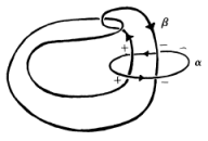
The linking number of the Whitehead link(Figure  4) below can be calculated as;

Refer to caption
Figure 4:
lk(α,β)=12(1+111)=0𝑙𝑘𝛼𝛽1211110lk(\alpha,\beta)=\frac{1}{2}(1+1-1-1)=0

The above example gives the linking number of the Whitehead link, and even though it has linking number zero, it is linked.

Remark 2.3.

The linking number is an invariant of an oriented link of two components. We can check this by how Reidemeister moves affect the linking number.

A move of type I𝐼I generates a new crossing of a link component with itself. These are ignored in computing the linking number. Thus there is no change to this quantity.

A move of type II𝐼𝐼II generates two crossings, both involving the same component or components of the link. One crossing will be assigned +11+1 and the other will be assigned 11-1.Thus even if the crossing involve both components of the link, the sum of the numbers will not change.

A move of type III𝐼𝐼𝐼III merely alters the relative positions of the three crossing without changing the components or orientation involved. Hence, there is no change to the linking number

2.4 Alexander Polynomial

In 1928, J.W Alexander introduced a polynomial invariant that is straight forward to compute,has a moderately easy proof and yet is fairly good at distinguishing among different knots. In his approach, the knot diagram gives entries of a matrix whose determinant is the Alexander Polynomial[3]. Alexander determined the entries of a matrix from the crossings and arcs of the diagram.

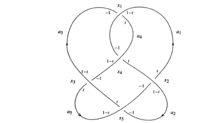
At each crossing of the knot diagram, the breaks in the lower strand divide the curve into arcs that begin and end at crossing. Since each arc has two ends and each crossing involves the ends of the arcs, the number of arcs is equal to the number of crossing. In our notation, we index the crossing x1,x2,,xnsubscript𝑥1subscript𝑥2subscript𝑥𝑛x_{1},x_{2},...,x_{n} and index the arcs a1,a2,,ansubscript𝑎1subscript𝑎2subscript𝑎𝑛a_{1},a_{2},...,a_{n}. Next we choose an orientation of the knot. As you travel around the knot, stand on the overpass of each crossing and face in the direction of the orientation. Label the three strands of the knot diagram that form this crossing: put 1t1𝑡1-t on the overpass itself, label the end of the underpass arc on your left t𝑡t and label the end of the underpass arc on your right with -1. We then form an n×n𝑛𝑛n\times n matrix by writing the label on arc ajsubscript𝑎𝑗a_{j} at crossing xisubscript𝑥𝑖x_{i} as ij𝑖𝑗ij-entry of the matrix. If an arc has more than one of its labels at the crossing, put the sum of the labels at the entry of the matrix. If the arc is not involved in forming the crossing, put a 00 as the entry. This matrix is the crossing/arc matrix of the knot diagram. Next we delete one column and one row of the matrix and compute the determinant of the resulting (n1)×(n1)𝑛1𝑛1(n-1)\times(n-1) matrix. This will be a polynomial in the variable t𝑡t which depends on quite a few choices: the index system for the crossing and arcs, the orientation of the knot, the selection of a row and column to eliminate, to say nothing of the choice of the knot diagram. Alexander’s amazing discovery is that although these choices may produce different polynomials, any one of them will be plus or minus a power of t𝑡t times any other. Thus if we normalize the polynomial to have a positive constant term, the resulting Alexander Polynomial will be a knot invariant.

In [16] one can find the proof showing that the Alexander polynomial does not depend on the indexing of crossings and arcs. It does not also depend on the row and column eliminated from the crossing/arc matrix. In the same text one can see how to use the Skein relation discovered by John Conway in 196919691969 to compute the Alexander polynomial. The Alexander polynomial is invariant up to multiplication by ±tNplus-or-minussuperscript𝑡𝑁\pm t^{N} where N𝑁N is some integer.

Example 2.10 ([16]).
Refer to caption
Figure 5:

The crossing/arc matrix of the above oriented knot diagram(Figure  5 ) is given as:

(1t01t0t1t001001t1t1t01t001t01t)matrix1𝑡01𝑡0𝑡1𝑡001001𝑡1𝑡1𝑡01𝑡001𝑡01𝑡\begin{pmatrix}1-t&0&-1&t&0\\ t&1-t&0&0&-1\\ 0&0&1-t&-1&t\\ -1&t&0&1-t&0\\ 0&-1&t&0&1-t\end{pmatrix}

We then eliminate the fourth row and the last column and compute the determinant of the resulting 4×4444\times 4 matrix as:

det(1t01tt1t00001t101t0)𝑑𝑒𝑡matrix1𝑡01𝑡𝑡1𝑡00001𝑡101𝑡0\displaystyle det\begin{pmatrix}1-t&0&-1&t\\ t&1-t&0&0\\ 0&0&1-t&-1\\ 0&-1&t&0\end{pmatrix} =\displaystyle= tdet(01t01t11t0)+(1t)det(1t0001t11t0)𝑡𝑑𝑒𝑡matrix01𝑡01𝑡11𝑡01𝑡𝑑𝑒𝑡matrix1𝑡0001𝑡11𝑡0\displaystyle-tdet\begin{pmatrix}0&-1&t\\ 0&1-t&-1\\ -1&t&0\end{pmatrix}+(1-t)det\begin{pmatrix}1-t&0&0\\ 0&1-t&-1\\ -1&t&0\end{pmatrix}
=\displaystyle= t(t1t2)+t(1t)2=2t33t2+2t𝑡𝑡1superscript𝑡2𝑡superscript1𝑡22superscript𝑡33superscript𝑡22𝑡\displaystyle-t(t-1-t^{2})+t(1-t)^{2}=2t^{3}-3t^{2}+2t

Finally we multiply the resulting determinant by t1superscript𝑡1t^{-1} to normalize this polynomial in order to have a positive constant term. Thus 2t23t+22superscript𝑡23𝑡22t^{2}-3t+2 is the Alexander polynomial of this knot.

3 The Kauffman Bracket Polynomial Model of the Jones Polynomial

In this chapter, we focus on the definition of the Jones polynomial as constructed by Louis Kauffman in terms of his bracket polynomial. The bracket polynomial is in general a Laurent polynomial since it contains terms with negative exponent.

3.1 The Rules for the Kauffman Bracket Polynomial

The Kauffman bracket polynomial of a regular projection of a link, say L𝐿L is denoted by Ldelimited-⟨⟩𝐿\langle L\rangle and L[A,A1]delimited-⟨⟩𝐿𝐴superscript𝐴1\langle L\rangle\in\mathbb{Z}[A,A^{-1}] [10]. It satisfies the following rules;

  1. 1.

    The bracket of a diagram consisting of n𝑛n disjoint simple closed curves in the plane is δn1superscript𝛿𝑛1\delta^{n-1}, where δ=A2A2𝛿superscript𝐴2superscript𝐴2\delta=-A^{-2}-A^{2}.

  2. 2.

    [Uncaptioned image]=A[Uncaptioned image]+A1[Uncaptioned image]delimited-⟨⟩[Uncaptioned image]𝐴delimited-⟨⟩[Uncaptioned image]superscript𝐴1delimited-⟨⟩[Uncaptioned image]\left\langle\raisebox{-6.00006pt}{\includegraphics[scale={0.3}]{t55.PNG}}\right\rangle=A\left\langle\raisebox{-6.00006pt}{\includegraphics[scale={0.3}]{t24.PNG}}\right\rangle+A^{-1}\left\langle\raisebox{-6.00006pt}{\includegraphics[scale={0.3}]{t21.PNG}}\right\rangle

    [Uncaptioned image]=A[Uncaptioned image]+A1[Uncaptioned image]delimited-⟨⟩[Uncaptioned image]𝐴delimited-⟨⟩[Uncaptioned image]superscript𝐴1delimited-⟨⟩[Uncaptioned image]\left\langle\raisebox{-6.00006pt}{\includegraphics[scale={0.3}]{t56.PNG}}\right\rangle=A\left\langle\raisebox{-6.00006pt}{\includegraphics[scale={0.3}]{t21.PNG}}\right\rangle+A^{-1}\left\langle\raisebox{-6.00006pt}{\includegraphics[scale={0.3}]{t24.PNG}}\right\rangle

  3. 3.

    LO=δLdelimited-⟨⟩square-union𝐿𝑂𝛿delimited-⟨⟩𝐿\left\langle L\sqcup O\right\rangle=\delta\left\langle L\right\rangle, where O𝑂O is a simple closed curve.

A useful consequence of rule 222 is the following switching formula;

A[Uncaptioned image]A1[Uncaptioned image]=(A2A2)[Uncaptioned image]𝐴delimited-⟨⟩[Uncaptioned image]superscript𝐴1delimited-⟨⟩[Uncaptioned image]superscript𝐴2superscript𝐴2delimited-⟨⟩[Uncaptioned image]A\left\langle\raisebox{-6.00006pt}{\includegraphics[scale={0.3}]{t56.PNG}}\right\rangle-A^{-1}\left\langle\raisebox{-6.00006pt}{\includegraphics[scale={0.3}]{t55.PNG}}\right\rangle=(A^{2}-A^{-2})\left\langle\raisebox{-6.00006pt}{\includegraphics[scale={0.3}]{t21.PNG}}\right\rangle (2)

This formula is useful since some computations will simplify quite quickly with the proper choices of switching and smoothing.

At this point we check the invariance of the bracket polynomial using the Reidemeister moves. We first consider the type II Reidemeister move;

[Uncaptioned image]delimited-⟨⟩[Uncaptioned image]\displaystyle\left\langle\raisebox{-6.00006pt}{\includegraphics[scale={0.4}]{j5.PNG}}\right\rangle =\displaystyle= A[Uncaptioned image]+A1[Uncaptioned image]𝐴delimited-⟨⟩[Uncaptioned image]superscript𝐴1delimited-⟨⟩[Uncaptioned image]\displaystyle A\left\langle\raisebox{-6.00006pt}{\includegraphics[scale={0.4}]{j6.PNG}}\right\rangle+A^{-1}\left\langle\raisebox{-6.00006pt}{\includegraphics[scale={0.4}]{j7.PNG}}\right\rangle
=\displaystyle= A[A[Uncaptioned image]+A1[Uncaptioned image]]+A1[A[Uncaptioned image]+A1[Uncaptioned image]]𝐴delimited-[]𝐴delimited-⟨⟩[Uncaptioned image]superscript𝐴1delimited-⟨⟩[Uncaptioned image]superscript𝐴1delimited-[]𝐴delimited-⟨⟩[Uncaptioned image]superscript𝐴1delimited-⟨⟩[Uncaptioned image]\displaystyle A\left[A\left\langle\raisebox{-6.00006pt}{\includegraphics[scale={0.4}]{j11.PNG}}\right\rangle+A^{-1}\left\langle\raisebox{-6.00006pt}{\includegraphics[scale={0.4}]{j8.PNG}}\right\rangle\right]+A^{-1}\left[A\left\langle\raisebox{-6.00006pt}{\includegraphics[scale={0.4}]{j9.PNG}}\right\rangle+A^{-1}\left\langle\raisebox{-6.00006pt}{\includegraphics[scale={0.4}]{j10.PNG}}\right\rangle\right]
=\displaystyle= A2[Uncaptioned image]+[Uncaptioned image]+[Uncaptioned image]+A2[Uncaptioned image]superscript𝐴2delimited-⟨⟩[Uncaptioned image]delimited-⟨⟩[Uncaptioned image]delimited-⟨⟩[Uncaptioned image]superscript𝐴2delimited-⟨⟩[Uncaptioned image]\displaystyle A^{2}\left\langle\raisebox{-6.00006pt}{\includegraphics[scale={0.4}]{j11.PNG}}\right\rangle+\left\langle\raisebox{-6.00006pt}{\includegraphics[scale={0.4}]{j8.PNG}}\right\rangle+\left\langle\raisebox{-6.00006pt}{\includegraphics[scale={0.4}]{j9.PNG}}\right\rangle+A^{-2}\left\langle\raisebox{-6.00006pt}{\includegraphics[scale={0.4}]{j10.PNG}}\right\rangle
=\displaystyle= A2[Uncaptioned image]+(A2A2)[Uncaptioned image]+[Uncaptioned image]+A2[Uncaptioned image]superscript𝐴2delimited-⟨⟩[Uncaptioned image]superscript𝐴2superscript𝐴2delimited-⟨⟩[Uncaptioned image]delimited-⟨⟩[Uncaptioned image]superscript𝐴2delimited-⟨⟩[Uncaptioned image]\displaystyle A^{2}\left\langle\raisebox{-6.00006pt}{\includegraphics[scale={0.4}]{j11.PNG}}\right\rangle+(-A^{2}-A^{-2})\left\langle\raisebox{-6.00006pt}{\includegraphics[scale={0.4}]{j11.PNG}}\right\rangle+\left\langle\raisebox{-6.00006pt}{\includegraphics[scale={0.4}]{j9.PNG}}\right\rangle+A^{-2}\left\langle\raisebox{-6.00006pt}{\includegraphics[scale={0.4}]{j10.PNG}}\right\rangle
=\displaystyle= (A2A2A2+A2)[Uncaptioned image]+[Uncaptioned image]superscript𝐴2superscript𝐴2superscript𝐴2superscript𝐴2delimited-⟨⟩[Uncaptioned image]delimited-⟨⟩[Uncaptioned image]\displaystyle(A^{2}-A^{2}-A^{-2}+A^{-2})\left\langle\raisebox{-6.00006pt}{\includegraphics[scale={0.4}]{j11.PNG}}\right\rangle+\left\langle\raisebox{-6.00006pt}{\includegraphics[scale={0.25}]{t24.PNG}}\right\rangle
=\displaystyle= [Uncaptioned image]delimited-⟨⟩[Uncaptioned image]\displaystyle\left\langle\raisebox{-6.00006pt}{\includegraphics[scale={0.25}]{t24.PNG}}\right\rangle

Checking the invariance under type III moves is easy since we can use the invariance under type II moves to slide some arcs around a little.

[Uncaptioned image]delimited-⟨⟩[Uncaptioned image]\displaystyle\left\langle\raisebox{-6.00006pt}{\includegraphics[scale={0.4}]{j12.PNG}}\right\rangle =\displaystyle= A[Uncaptioned image]+A1[Uncaptioned image]𝐴delimited-⟨⟩[Uncaptioned image]superscript𝐴1delimited-⟨⟩[Uncaptioned image]\displaystyle A\left\langle\raisebox{-6.00006pt}{\includegraphics[scale={0.4}]{j13.PNG}}\right\rangle+A^{-1}\left\langle\raisebox{-6.00006pt}{\includegraphics[scale={0.4}]{j14.PNG}}\right\rangle
=\displaystyle= A[Uncaptioned image]+A1[Uncaptioned image]𝐴delimited-⟨⟩[Uncaptioned image]superscript𝐴1delimited-⟨⟩[Uncaptioned image]\displaystyle A\left\langle\raisebox{-6.00006pt}{\includegraphics[scale={0.4}]{j15.PNG}}\right\rangle+A^{-1}\left\langle\raisebox{-6.00006pt}{\includegraphics[scale={0.4}]{j16.PNG}}\right\rangle
=\displaystyle= A[Uncaptioned image]+A1[Uncaptioned image]𝐴delimited-⟨⟩[Uncaptioned image]superscript𝐴1delimited-⟨⟩[Uncaptioned image]\displaystyle A\left\langle\raisebox{-6.00006pt}{\includegraphics[scale={0.4}]{j17.PNG}}\right\rangle+A^{-1}\left\langle\raisebox{-6.00006pt}{\includegraphics[scale={0.4}]{j18.PNG}}\right\rangle
=\displaystyle= [Uncaptioned image]delimited-⟨⟩[Uncaptioned image]\displaystyle\left\langle\raisebox{-6.00006pt}{\includegraphics[scale={0.4}]{j19.PNG}}\right\rangle
Definition 3.1.

Two knot or link diagrams are defined to be regular isotopic if one can be obtained from the other by a combination of planar isotopy and the second and third Reidemeister moves.

The bracket polynomial is therefore a regular isotopy invariant as it is not invariant under type I Reidemeister moves. This can be seen as follows;

For the curl with a right-handed crossing we have,

[Uncaptioned image]delimited-⟨⟩[Uncaptioned image]\displaystyle\left\langle\raisebox{-6.00006pt}{\includegraphics[scale={0.4}]{j1.PNG}}\right\rangle =\displaystyle= A[Uncaptioned image]+A1[Uncaptioned image]𝐴delimited-⟨⟩[Uncaptioned image]superscript𝐴1delimited-⟨⟩[Uncaptioned image]\displaystyle A\left\langle\raisebox{-6.00006pt}{\includegraphics[scale={0.4}]{j2.PNG}}\right\rangle+A^{-1}\left\langle\raisebox{-6.00006pt}{\includegraphics[scale={0.4}]{j3.PNG}}\right\rangle
=\displaystyle= A(A2A2)[Uncaptioned image]+A1[Uncaptioned image]𝐴superscript𝐴2superscript𝐴2delimited-⟨⟩[Uncaptioned image]superscript𝐴1delimited-⟨⟩[Uncaptioned image]\displaystyle A(-A^{-2}-A^{2})\left\langle\raisebox{-6.00006pt}{\includegraphics[scale={0.4}]{j4.PNG}}\right\rangle+A^{-1}\left\langle\raisebox{-6.00006pt}{\includegraphics[scale={0.4}]{j3.PNG}}\right\rangle
=\displaystyle= (A3A1+A1)[Uncaptioned image]superscript𝐴3superscript𝐴1superscript𝐴1delimited-⟨⟩[Uncaptioned image]\displaystyle(-A^{3}-A^{-1}+A^{-1})\left\langle\raisebox{-6.00006pt}{\includegraphics[scale={0.4}]{j4.PNG}}\right\rangle
=\displaystyle= A3[Uncaptioned image]superscript𝐴3delimited-⟨⟩[Uncaptioned image]\displaystyle-A^{3}\left\langle\raisebox{-6.00006pt}{\includegraphics[scale={0.4}]{j4.PNG}}\right\rangle

and for the curl with a left-handed crossing we have,

[Uncaptioned image]delimited-⟨⟩[Uncaptioned image]\displaystyle\left\langle\raisebox{-6.00006pt}{\includegraphics[scale={0.4}]{j23.PNG}}\right\rangle =\displaystyle= A[Uncaptioned image]+A1[Uncaptioned image]𝐴delimited-⟨⟩[Uncaptioned image]superscript𝐴1delimited-⟨⟩[Uncaptioned image]\displaystyle A\left\langle\raisebox{-6.00006pt}{\includegraphics[scale={0.4}]{j3.PNG}}\right\rangle+A^{-1}\left\langle\raisebox{-6.00006pt}{\includegraphics[scale={0.4}]{j2.PNG}}\right\rangle
=\displaystyle= A[Uncaptioned image]+A1(A2A2)[Uncaptioned image]𝐴delimited-⟨⟩[Uncaptioned image]superscript𝐴1superscript𝐴2superscript𝐴2delimited-⟨⟩[Uncaptioned image]\displaystyle A\left\langle\raisebox{-6.00006pt}{\includegraphics[scale={0.4}]{j3.PNG}}\right\rangle+A^{-1}(-A^{-2}-A^{2})\left\langle\raisebox{-6.00006pt}{\includegraphics[scale={0.4}]{j4.PNG}}\right\rangle
=\displaystyle= (AAA3)[Uncaptioned image]𝐴𝐴superscript𝐴3delimited-⟨⟩[Uncaptioned image]\displaystyle(A-A-A^{-3})\left\langle\raisebox{-6.00006pt}{\includegraphics[scale={0.4}]{j4.PNG}}\right\rangle
=\displaystyle= A3[Uncaptioned image]superscript𝐴3delimited-⟨⟩[Uncaptioned image]\displaystyle-A^{-3}\left\langle\raisebox{-6.00006pt}{\includegraphics[scale={0.4}]{j4.PNG}}\right\rangle
Example 3.2.

The first diagram in Figure  6 indicated as K𝐾K is the right-handed trefoil. We wish to compute its bracket polynomial.
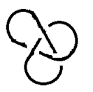
Refer to caption
(a) K𝐾K
Refer to caption
(b) Ksuperscript𝐾K^{\prime}
Refer to caption
(c) K′′superscript𝐾′′K^{\prime\prime}
Figure 6:

By switching and smoothening one of its crossings, we can write a switching formula as in Equation  (2),

A1KAK=(A2A2)K′′superscript𝐴1delimited-⟨⟩𝐾𝐴delimited-⟨⟩superscript𝐾superscript𝐴2superscript𝐴2delimited-⟨⟩superscript𝐾′′A^{-1}\langle K\rangle-A\langle K^{\prime}\rangle=(A^{-2}-A^{2})\langle K^{\prime\prime}\rangle (3)

Applying regular isotopy to the diagram Ksuperscript𝐾K^{\prime} we obtain an unknot with a right-handed crossing, so then K=A3delimited-⟨⟩superscript𝐾superscript𝐴3\langle K^{\prime}\rangle=-A^{3}. Similarly the diagram K′′superscript𝐾′′K^{\prime\prime} is an unknot with two left-handed crossings so then K′′=(A3)2=A6delimited-⟨⟩superscript𝐾′′superscriptsuperscript𝐴32superscript𝐴6\langle K^{\prime\prime}\rangle=(-A^{-3})^{2}=A^{-6}.We therefore obtain,

A1KA(A3)=(A2A2)(A6)superscript𝐴1delimited-⟨⟩𝐾𝐴superscript𝐴3superscript𝐴2superscript𝐴2superscript𝐴6A^{-1}\langle K\rangle-A(-A^{3})=(A^{-2}-A^{2})(A^{-6})

Hence

A1K=A8A4A4superscript𝐴1delimited-⟨⟩𝐾superscript𝐴8superscript𝐴4superscript𝐴4A^{-1}\langle K\rangle=A^{-8}-A^{-4}-A^{4}

So

K=A7A3A5delimited-⟨⟩𝐾superscript𝐴7superscript𝐴3superscript𝐴5\langle K\rangle=A^{-7}-A^{-3}-A^{5}
Definition 3.3.

The writhe, w(L)𝑤𝐿w(L) of the regular projection L𝐿L of a link is the number of right-handed crossings minus the number of left-handed crossings.

As we have seen, a type I𝐼I move that eliminates a right-handed crossing will introduce a factor A3superscript𝐴3-A^{3} into the bracket and a type I𝐼I move that eliminates a left-handed crossing will introduce a factor A3superscript𝐴3-A^{-3} into the bracket.

The bracket polynomial of the regular projection L𝐿L of a link can thus be normalized by multiplying by the factor (A)3w(L)superscript𝐴3𝑤𝐿(-A)^{-3w(L)}. The normalized bracket polynomial denoted by XLsubscript𝑋𝐿X_{L} is therefore written as;

XL=(A)3w(L)Lsubscript𝑋𝐿superscript𝐴3𝑤𝐿delimited-⟨⟩𝐿X_{L}=(-A)^{-3w(L)}\langle L\rangle (4)

Let L𝐿L and Lsuperscript𝐿L^{\prime} differ by a single first Reidemeister move,

XLsubscript𝑋𝐿\displaystyle X_{L} =\displaystyle= (A)3w(L)Lsuperscript𝐴3𝑤𝐿delimited-⟨⟩𝐿\displaystyle(-A)^{-3w(L)}\langle L\rangle
=\displaystyle= (A)3(w(L)+1)(A3)Lsuperscript𝐴3𝑤superscript𝐿1superscript𝐴3delimited-⟨⟩superscript𝐿\displaystyle(-A)^{-3(w(L^{\prime})+1)}(-A^{3})\langle L^{\prime}\rangle
=\displaystyle= (A)3w(L)(A3)(A3)Lsuperscript𝐴3𝑤superscript𝐿superscript𝐴3superscript𝐴3delimited-⟨⟩superscript𝐿\displaystyle(-A)^{-3w(L^{\prime})}\cdot(-A^{-3})\cdot(-A^{3})\langle L^{\prime}\rangle
=\displaystyle= (A)3w(L)Lsuperscript𝐴3𝑤superscript𝐿delimited-⟨⟩superscript𝐿\displaystyle(-A)^{-3w(L^{\prime})}\langle L^{\prime}\rangle
=\displaystyle= XLsubscript𝑋superscript𝐿\displaystyle X_{L^{\prime}}

We have shown that the bracket polynomial is invariant under type II𝐼𝐼II and type III𝐼𝐼𝐼III Reidemeister moves. Also by direct verification we can as well see that the writhe is invariant under type II and type III Reidemeister moves. We can therefore conclude that the normalized bracket polynomial is a knot invariant.

Definition 3.4.

The Jones polynomial VLsubscript𝑉𝐿V_{L} of a link L𝐿L is obtained by making the substitution A=t14𝐴superscript𝑡14A=t^{-\frac{1}{4}} in the polynomial XLsubscript𝑋𝐿X_{L}.

The writhe of the trefoil diagram, K𝐾K in Figure  6 is +33+3 so then its normalized bracket polynomial is given as,

XK(A)subscript𝑋𝐾𝐴\displaystyle X_{K}(A) =\displaystyle= (A)3(3)(A7A3A5)superscript𝐴33superscript𝐴7superscript𝐴3superscript𝐴5\displaystyle(-A)^{-3(3)}(A^{-7}-A^{-3}-A^{5})
=\displaystyle= A16+A12+A4superscript𝐴16superscript𝐴12superscript𝐴4\displaystyle-A^{-16}+A^{-12}+A^{-4}

The Jones polynomial of the right-handed trefoil is therefore

VK(t)=XK(t14)=t4+t3+tsubscript𝑉𝐾𝑡subscript𝑋𝐾superscript𝑡14superscript𝑡4superscript𝑡3𝑡V_{K}(t)=X_{K}(t^{-\frac{1}{4}})=-t^{4}+t^{3}+t (5)

3.2 Calculating the Bracket Polynomial of Double Stranded Knots and Links.

In this section, we apply the basic bracket expansion formula to create a switching formula for calculating double stranded links and doubles of knots.(refer to [13, 8])

By expanding on all four vertices, one finds the following formula for the bracket invariant;

[Uncaptioned image]delimited-⟨⟩[Uncaptioned image]\displaystyle\left\langle\raisebox{-6.00006pt}{\includegraphics[scale={0.2}]{t50.PNG}}\right\rangle =\displaystyle= A4[Uncaptioned image]+A4[Uncaptioned image]+A2[[Uncaptioned image]+[Uncaptioned image]]+A2[[Uncaptioned image]+[Uncaptioned image]]superscript𝐴4delimited-⟨⟩[Uncaptioned image]superscript𝐴4delimited-⟨⟩[Uncaptioned image]superscript𝐴2delimited-[]delimited-⟨⟩[Uncaptioned image]delimited-⟨⟩[Uncaptioned image]superscript𝐴2delimited-[]delimited-⟨⟩[Uncaptioned image]delimited-⟨⟩[Uncaptioned image]\displaystyle A^{4}\left\langle\raisebox{-6.00006pt}{\includegraphics[scale={0.2}]{s6.PNG}}\right\rangle+A^{-4}\left\langle\raisebox{-6.00006pt}{\includegraphics[scale={0.2}]{s10.PNG}}\right\rangle+A^{2}\left[\left\langle\raisebox{-6.00006pt}{\includegraphics[scale={0.2}]{s7.PNG}}\right\rangle+\left\langle\raisebox{-6.00006pt}{\includegraphics[scale={0.2}]{s11.PNG}}\right\rangle\right]+A^{-2}\left[\left\langle\raisebox{-6.00006pt}{\includegraphics[scale={0.2}]{s18.PNG}}\right\rangle+\left\langle\raisebox{-6.00006pt}{\includegraphics[scale={0.2}]{s21.PNG}}\right\rangle\right]
+\displaystyle+ (A2+A2)[Uncaptioned image]+A0[[Uncaptioned image]+[Uncaptioned image]+[Uncaptioned image]+[Uncaptioned image]+[Uncaptioned image]]superscript𝐴2superscript𝐴2delimited-⟨⟩[Uncaptioned image]superscript𝐴0delimited-[]delimited-⟨⟩[Uncaptioned image]delimited-⟨⟩[Uncaptioned image]delimited-⟨⟩[Uncaptioned image]delimited-⟨⟩[Uncaptioned image]delimited-⟨⟩[Uncaptioned image]\displaystyle(A^{2}+A^{-2})\left\langle\raisebox{-6.00006pt}{\includegraphics[scale={0.2}]{s24.PNG}}\right\rangle+A^{0}\left[\left\langle\raisebox{-6.00006pt}{\includegraphics[scale={0.2}]{s8.PNG}}\right\rangle+\left\langle\raisebox{-6.00006pt}{\includegraphics[scale={0.2}]{s19.PNG}}\right\rangle+\left\langle\raisebox{-6.00006pt}{\includegraphics[scale={0.2}]{s12.PNG}}\right\rangle+\left\langle\raisebox{-6.00006pt}{\includegraphics[scale={0.2}]{s22.PNG}}\right\rangle+\left\langle\raisebox{-6.00006pt}{\includegraphics[scale={0.2}]{s25.PNG}}\right\rangle\right]
[Uncaptioned image]delimited-⟨⟩[Uncaptioned image]\displaystyle\left\langle\raisebox{-6.00006pt}{\includegraphics[scale={0.2}]{t51.PNG}}\right\rangle =\displaystyle= A4[Uncaptioned image]+A4[Uncaptioned image]+A2[[Uncaptioned image]+[Uncaptioned image]]+A2[[Uncaptioned image]+[Uncaptioned image]]superscript𝐴4delimited-⟨⟩[Uncaptioned image]superscript𝐴4delimited-⟨⟩[Uncaptioned image]superscript𝐴2delimited-[]delimited-⟨⟩[Uncaptioned image]delimited-⟨⟩[Uncaptioned image]superscript𝐴2delimited-[]delimited-⟨⟩[Uncaptioned image]delimited-⟨⟩[Uncaptioned image]\displaystyle A^{4}\left\langle\raisebox{-6.00006pt}{\includegraphics[scale={0.2}]{s10.PNG}}\right\rangle+A^{-4}\left\langle\raisebox{-6.00006pt}{\includegraphics[scale={0.2}]{s6.PNG}}\right\rangle+A^{2}\left[\left\langle\raisebox{-6.00006pt}{\includegraphics[scale={0.2}]{s18.PNG}}\right\rangle+\left\langle\raisebox{-6.00006pt}{\includegraphics[scale={0.2}]{s21.PNG}}\right\rangle\right]+A^{-2}\left[\left\langle\raisebox{-6.00006pt}{\includegraphics[scale={0.2}]{s7.PNG}}\right\rangle+\left\langle\raisebox{-6.00006pt}{\includegraphics[scale={0.2}]{s11.PNG}}\right\rangle\right]
+\displaystyle+ (A2+A2)[Uncaptioned image]+A0[[Uncaptioned image]+[Uncaptioned image]+[Uncaptioned image]+[Uncaptioned image]+[Uncaptioned image]]superscript𝐴2superscript𝐴2delimited-⟨⟩[Uncaptioned image]superscript𝐴0delimited-[]delimited-⟨⟩[Uncaptioned image]delimited-⟨⟩[Uncaptioned image]delimited-⟨⟩[Uncaptioned image]delimited-⟨⟩[Uncaptioned image]delimited-⟨⟩[Uncaptioned image]\displaystyle(A^{2}+A^{-2})\left\langle\raisebox{-6.00006pt}{\includegraphics[scale={0.2}]{s24.PNG}}\right\rangle+A^{0}\left[\left\langle\raisebox{-6.00006pt}{\includegraphics[scale={0.2}]{s8.PNG}}\right\rangle+\left\langle\raisebox{-6.00006pt}{\includegraphics[scale={0.2}]{s19.PNG}}\right\rangle+\left\langle\raisebox{-6.00006pt}{\includegraphics[scale={0.2}]{s12.PNG}}\right\rangle+\left\langle\raisebox{-6.00006pt}{\includegraphics[scale={0.2}]{s22.PNG}}\right\rangle+\left\langle\raisebox{-6.00006pt}{\includegraphics[scale={0.2}]{s25.PNG}}\right\rangle\right]

The above two expansion formula immediately leads to the switching identity;

[Uncaptioned image][Uncaptioned image]delimited-⟨⟩[Uncaptioned image]delimited-⟨⟩[Uncaptioned image]\displaystyle\left\langle\raisebox{-6.00006pt}{\includegraphics[scale={0.2}]{t50.PNG}}\right\rangle-\left\langle\raisebox{-6.00006pt}{\includegraphics[scale={0.2}]{t51.PNG}}\right\rangle =\displaystyle= (A4A4)[[Uncaptioned image][Uncaptioned image]]+(A2A2)[[Uncaptioned image]+[Uncaptioned image]\displaystyle(A^{4}-A^{-4})\left[\left\langle\raisebox{-6.00006pt}{\includegraphics[scale={0.2}]{s6.PNG}}\right\rangle-\left\langle\raisebox{-6.00006pt}{\includegraphics[scale={0.2}]{s10.PNG}}\right\rangle\right]+(A^{2}-A^{-2})[\left\langle\raisebox{-6.00006pt}{\includegraphics[scale={0.2}]{s7.PNG}}\right\rangle+\left\langle\raisebox{-6.00006pt}{\includegraphics[scale={0.2}]{s11.PNG}}\right\rangle
\displaystyle- [Uncaptioned image][Uncaptioned image]]\displaystyle\left\langle\raisebox{-6.00006pt}{\includegraphics[scale={0.2}]{s18.PNG}}\right\rangle-\left\langle\raisebox{-6.00006pt}{\includegraphics[scale={0.2}]{s21.PNG}}\right\rangle]

This identity will help us to compute the bracket polynomial and eventually the Jones polynomial of a double stranded link.

In other to do the calculation with much ease, we adapt a short hand notation of the above formula.We have that,

[Uncaptioned image]=[Uncaptioned image]delimited-⟨⟩[Uncaptioned image]delimited-⟨⟩delimited-⟨⟩[Uncaptioned image]\left\langle\raisebox{-3.99994pt}{\includegraphics[scale={0.3}]{s82.PNG}}\right\rangle=\left\langle\left\langle\raisebox{-3.99994pt}{\includegraphics[scale={0.4}]{s83.PNG}}\right\rangle\right\rangle (6)

and

[Uncaptioned image]=[Uncaptioned image]delimited-⟨⟩[Uncaptioned image]delimited-⟨⟩delimited-⟨⟩[Uncaptioned image]\left\langle\raisebox{-6.00006pt}{\includegraphics[scale={0.3}]{s24.PNG}}\right\rangle=\left\langle\left\langle\raisebox{-6.00006pt}{\includegraphics[scale={0.3}]{s16.PNG}}\right\rangle\right\rangle (7)

while

[Uncaptioned image]=[Uncaptioned image]delimited-⟨⟩[Uncaptioned image]delimited-⟨⟩delimited-⟨⟩[Uncaptioned image]\left\langle\raisebox{-6.00006pt}{\includegraphics[scale={0.2}]{s8.PNG}}\right\rangle=\left\langle\left\langle\raisebox{-6.00006pt}{\includegraphics[scale={0.3}]{s68.PNG}}\right\rangle\right\rangle (8)

Our expansion formula will thus be written as;

[Uncaptioned image]delimited-⟨⟩delimited-⟨⟩[Uncaptioned image]\displaystyle\left\langle\left\langle\raisebox{-6.00006pt}{\includegraphics[scale={0.2}]{t52.PNG}}\right\rangle\right\rangle =\displaystyle= A4[Uncaptioned image]+A4[Uncaptioned image]+A2[[Uncaptioned image]+[Uncaptioned image]]superscript𝐴4delimited-⟨⟩delimited-⟨⟩[Uncaptioned image]superscript𝐴4delimited-⟨⟩delimited-⟨⟩[Uncaptioned image]superscript𝐴2delimited-[]delimited-⟨⟩delimited-⟨⟩[Uncaptioned image]delimited-⟨⟩delimited-⟨⟩[Uncaptioned image]\displaystyle A^{4}\left\langle\left\langle\raisebox{-6.00006pt}{\includegraphics[scale={0.3}]{s1.PNG}}\right\rangle\right\rangle+A^{-4}\left\langle\left\langle\raisebox{-6.00006pt}{\includegraphics[scale={0.3}]{s2.PNG}}\right\rangle\right\rangle+A^{2}\left[\left\langle\left\langle\raisebox{-6.00006pt}{\includegraphics[scale={0.3}]{s3.PNG}}\right\rangle\right\rangle+\left\langle\left\langle\raisebox{-6.00006pt}{\includegraphics[scale={0.3}]{s5.PNG}}\right\rangle\right\rangle\right]
+\displaystyle+ A2[[Uncaptioned image]+[Uncaptioned image]]+(A2+A2)[Uncaptioned image]superscript𝐴2delimited-[]delimited-⟨⟩delimited-⟨⟩[Uncaptioned image]delimited-⟨⟩delimited-⟨⟩[Uncaptioned image]superscript𝐴2superscript𝐴2delimited-⟨⟩delimited-⟨⟩[Uncaptioned image]\displaystyle A^{-2}\left[\left\langle\left\langle\raisebox{-6.00006pt}{\includegraphics[scale={0.3}]{s9.PNG}}\right\rangle\right\rangle+\left\langle\left\langle\raisebox{-6.00006pt}{\includegraphics[scale={0.3}]{s4.PNG}}\right\rangle\right\rangle\right]+(A^{2}+A^{-2})\left\langle\left\langle\raisebox{-6.00006pt}{\includegraphics[scale={0.3}]{s68.PNG}}\right\rangle\right\rangle
+\displaystyle+ A0[[Uncaptioned image]+[Uncaptioned image]+[Uncaptioned image]+[Uncaptioned image]+[Uncaptioned image]]superscript𝐴0delimited-[]delimited-⟨⟩delimited-⟨⟩[Uncaptioned image]delimited-⟨⟩delimited-⟨⟩[Uncaptioned image]delimited-⟨⟩delimited-⟨⟩[Uncaptioned image]delimited-⟨⟩delimited-⟨⟩[Uncaptioned image]delimited-⟨⟩delimited-⟨⟩[Uncaptioned image]\displaystyle A^{0}\left[\left\langle\left\langle\raisebox{-6.00006pt}{\includegraphics[scale={0.25}]{s16.PNG}}\right\rangle\right\rangle+\left\langle\left\langle\raisebox{-6.00006pt}{\includegraphics[scale={0.25}]{s20.PNG}}\right\rangle\right\rangle+\left\langle\left\langle\raisebox{-6.00006pt}{\includegraphics[scale={0.25}]{s23.PNG}}\right\rangle\right\rangle+\left\langle\left\langle\raisebox{-6.00006pt}{\includegraphics[scale={0.25}]{s26.PNG}}\right\rangle\right\rangle+\left\langle\left\langle\raisebox{-6.00006pt}{\includegraphics[scale={0.25}]{s27.PNG}}\right\rangle\right\rangle\right]

Noting for example that,

[Uncaptioned image]=[Uncaptioned image]delimited-⟨⟩delimited-⟨⟩[Uncaptioned image]delimited-⟨⟩[Uncaptioned image]\left\langle\left\langle\raisebox{-6.00006pt}{\includegraphics[scale={0.25}]{s20.PNG}}\right\rangle\right\rangle=\left\langle\raisebox{-6.00006pt}{\includegraphics[scale={0.25}]{s19.PNG}}\right\rangle (9)
[Uncaptioned image][Uncaptioned image]delimited-⟨⟩delimited-⟨⟩[Uncaptioned image]delimited-⟨⟩delimited-⟨⟩[Uncaptioned image]\displaystyle\left\langle\left\langle\raisebox{-6.00006pt}{\includegraphics[scale={0.2}]{t52.PNG}}\right\rangle\right\rangle-\left\langle\left\langle\raisebox{-6.00006pt}{\includegraphics[scale={0.2}]{t53.PNG}}\right\rangle\right\rangle =\displaystyle= (A4A4)[[Uncaptioned image][Uncaptioned image]]superscript𝐴4superscript𝐴4delimited-[]delimited-⟨⟩delimited-⟨⟩[Uncaptioned image]delimited-⟨⟩delimited-⟨⟩[Uncaptioned image]\displaystyle(A^{4}-A^{-4})\left[\left\langle\left\langle\raisebox{-6.00006pt}{\includegraphics[scale={0.2}]{s1.PNG}}\right\rangle\right\rangle-\left\langle\left\langle\raisebox{-6.00006pt}{\includegraphics[scale={0.2}]{s2.PNG}}\right\rangle\right\rangle\right]
+\displaystyle+ (A2A2)[[Uncaptioned image]+[Uncaptioned image][Uncaptioned image][Uncaptioned image]]superscript𝐴2superscript𝐴2delimited-[]delimited-⟨⟩delimited-⟨⟩[Uncaptioned image]delimited-⟨⟩delimited-⟨⟩[Uncaptioned image]delimited-⟨⟩delimited-⟨⟩[Uncaptioned image]delimited-⟨⟩delimited-⟨⟩[Uncaptioned image]\displaystyle(A^{2}-A^{-2})\left[\left\langle\left\langle\raisebox{-6.00006pt}{\includegraphics[scale={0.2}]{s3.PNG}}\right\rangle\right\rangle+\left\langle\left\langle\raisebox{-6.00006pt}{\includegraphics[scale={0.2}]{s5.PNG}}\right\rangle\right\rangle-\left\langle\left\langle\raisebox{-6.00006pt}{\includegraphics[scale={0.2}]{s9.PNG}}\right\rangle\right\rangle-\left\langle\left\langle\raisebox{-6.00006pt}{\includegraphics[scale={0.2}]{s4.PNG}}\right\rangle\right\rangle\right]

Below are also some rules that can facilitate the calculation.

[Uncaptioned image]=A8[Uncaptioned image]+(A6A2)[Uncaptioned image]delimited-⟨⟩delimited-⟨⟩[Uncaptioned image]superscript𝐴8delimited-⟨⟩delimited-⟨⟩[Uncaptioned image]superscript𝐴6superscript𝐴2delimited-⟨⟩delimited-⟨⟩[Uncaptioned image]\left\langle\left\langle\raisebox{-3.00003pt}{\includegraphics[scale={0.6}]{s62.PNG}}\right\rangle\right\rangle=A^{8}\left\langle\left\langle\raisebox{-3.00003pt}{\includegraphics[scale={0.4}]{s69.PNG}}\right\rangle\right\rangle+(A^{6}-A^{2})\left\langle\left\langle\raisebox{-3.00003pt}{\includegraphics[scale={0.4}]{s67.PNG}}\right\rangle\right\rangle (10)
[Uncaptioned image]=A8[Uncaptioned image]+(A6A2)[Uncaptioned image]delimited-⟨⟩delimited-⟨⟩[Uncaptioned image]superscript𝐴8delimited-⟨⟩delimited-⟨⟩[Uncaptioned image]superscript𝐴6superscript𝐴2delimited-⟨⟩delimited-⟨⟩[Uncaptioned image]\left\langle\left\langle\raisebox{-6.00006pt}{\includegraphics[scale={0.6}]{s63.PNG}}\right\rangle\right\rangle=A^{-8}\left\langle\left\langle\raisebox{-3.00003pt}{\includegraphics[scale={0.4}]{s69.PNG}}\right\rangle\right\rangle+(A^{-6}-A^{-2})\left\langle\left\langle\raisebox{-3.00003pt}{\includegraphics[scale={0.4}]{s67.PNG}}\right\rangle\right\rangle (11)
[Uncaptioned image]=1delimited-⟨⟩delimited-⟨⟩[Uncaptioned image]1\left\langle\left\langle\raisebox{-3.00003pt}{\includegraphics[scale={0.6}]{s64.PNG}}\right\rangle\right\rangle=1 (12)
[Uncaptioned image]=δdelimited-⟨⟩delimited-⟨⟩[Uncaptioned image]𝛿\left\langle\left\langle\raisebox{-6.00006pt}{\includegraphics[scale={0.4}]{s70.PNG}}\right\rangle\right\rangle=\delta (13)
[Uncaptioned image][Uncaptioned image]=δ[Uncaptioned image]delimited-⟨⟩delimited-⟨⟩[Uncaptioned image][Uncaptioned image]𝛿delimited-⟨⟩delimited-⟨⟩[Uncaptioned image]\left\langle\left\langle\raisebox{-3.00003pt}{\includegraphics[scale={0.3}]{s64.PNG}}\raisebox{-6.00006pt}{\includegraphics[scale={0.6}]{s66.PNG}}\right\rangle\right\rangle=\delta\left\langle\left\langle\raisebox{-6.00006pt}{\includegraphics[scale={0.6}]{s66.PNG}}\right\rangle\right\rangle (14)
[Uncaptioned image]=δ2[Uncaptioned image]delimited-⟨⟩delimited-⟨⟩[Uncaptioned image]superscript𝛿2delimited-⟨⟩delimited-⟨⟩[Uncaptioned image]\left\langle\left\langle\raisebox{-6.00006pt}{\includegraphics[scale={0.6}]{s65.PNG}}\right\rangle\right\rangle=\delta^{2}\left\langle\left\langle\raisebox{-6.00006pt}{\includegraphics[scale={0.6}]{s66.PNG}}\right\rangle\right\rangle (15)
Example 3.5.

We wish to calculate the bracket polynomial of the 2-strand diagram of the standard Hopf link.

Let us note that ;

[Uncaptioned image]=[Uncaptioned image]=[Uncaptioned image]=δ3delimited-⟨⟩delimited-⟨⟩[Uncaptioned image]delimited-⟨⟩delimited-⟨⟩[Uncaptioned image]delimited-⟨⟩[Uncaptioned image]superscript𝛿3\left\langle\left\langle\raisebox{-5.0pt}{\includegraphics[scale={0.6}]{s59.PNG}}\right\rangle\right\rangle=\left\langle\left\langle\raisebox{-1.99997pt}{\includegraphics[scale={0.6}]{s58.PNG}}\right\rangle\right\rangle=\left\langle\raisebox{-1.99997pt}{\includegraphics[scale={0.6}]{s57.PNG}}\right\rangle=\delta^{3} (16)

Now applying the switching formula we have,

[Uncaptioned image][Uncaptioned image]delimited-⟨⟩delimited-⟨⟩[Uncaptioned image]delimited-⟨⟩delimited-⟨⟩[Uncaptioned image]\displaystyle\left\langle\left\langle\includegraphics[scale={0.4}]{s85.PNG}\right\rangle\right\rangle-\left\langle\left\langle\includegraphics[scale={0.4}]{s59.PNG}\right\rangle\right\rangle =\displaystyle= (A4A4)[[Uncaptioned image][Uncaptioned image]]superscript𝐴4superscript𝐴4delimited-[]delimited-⟨⟩delimited-⟨⟩[Uncaptioned image]delimited-⟨⟩delimited-⟨⟩[Uncaptioned image]\displaystyle(A^{4}-A^{-4})\left[\left\langle\left\langle\includegraphics[scale={0.6}]{s56.PNG}\right\rangle\right\rangle-\left\langle\left\langle\includegraphics[scale={0.6}]{s51.PNG}\right\rangle\right\rangle\right]
+\displaystyle+ (A2A2)[[Uncaptioned image]+[Uncaptioned image][Uncaptioned image][Uncaptioned image]]superscript𝐴2superscript𝐴2delimited-[]delimited-⟨⟩delimited-⟨⟩[Uncaptioned image]delimited-⟨⟩delimited-⟨⟩[Uncaptioned image]delimited-⟨⟩delimited-⟨⟩[Uncaptioned image]delimited-⟨⟩delimited-⟨⟩[Uncaptioned image]\displaystyle(A^{2}-A^{-2})\left[\left\langle\left\langle\raisebox{-5.0pt}{\includegraphics[scale={0.6}]{s52.PNG}}\right\rangle\right\rangle+\left\langle\left\langle\raisebox{-5.0pt}{\includegraphics[scale={0.6}]{s55.PNG}}\right\rangle\right\rangle-\left\langle\left\langle\raisebox{-5.0pt}{\includegraphics[scale={0.6}]{s84.PNG}}\right\rangle\right\rangle-\left\langle\left\langle\raisebox{-5.0pt}{\includegraphics[scale={0.6}]{s53.PNG}}\right\rangle\right\rangle\right]

Therefore,

[Uncaptioned image]=δ3+(A4A4)[[Uncaptioned image][Uncaptioned image]]delimited-⟨⟩delimited-⟨⟩[Uncaptioned image]superscript𝛿3superscript𝐴4superscript𝐴4delimited-[]delimited-⟨⟩delimited-⟨⟩[Uncaptioned image]delimited-⟨⟩delimited-⟨⟩[Uncaptioned image]\left\langle\left\langle\includegraphics[scale={0.6}]{s85.PNG}\right\rangle\right\rangle=\delta^{3}+(A^{4}-A^{-4})\left[\left\langle\left\langle\raisebox{-5.0pt}{\includegraphics[scale={0.6}]{s56.PNG}}\right\rangle\right\rangle-\left\langle\left\langle\raisebox{-5.0pt}{\includegraphics[scale={0.6}]{s51.PNG}}\right\rangle\right\rangle\right] (17)

We have that

[Uncaptioned image]delimited-⟨⟩delimited-⟨⟩[Uncaptioned image]\displaystyle\left\langle\left\langle\raisebox{-5.0pt}{\includegraphics[scale={0.5}]{s56.PNG}}\right\rangle\right\rangle =\displaystyle= A8[Uncaptioned image]+(A6A2)[Uncaptioned image]superscript𝐴8delimited-⟨⟩delimited-⟨⟩[Uncaptioned image]superscript𝐴6superscript𝐴2delimited-⟨⟩delimited-⟨⟩[Uncaptioned image]\displaystyle A^{8}\left\langle\left\langle\includegraphics[scale={0.3}]{s70.PNG}\right\rangle\right\rangle+(A^{6}-A^{2})\left\langle\left\langle\includegraphics[scale={0.3}]{s80.PNG}\right\rangle\right\rangle
=\displaystyle= A8(A2A2)+A6A2superscript𝐴8superscript𝐴2superscript𝐴2superscript𝐴6superscript𝐴2\displaystyle A^{8}(-A^{2}-A^{-2})+A^{6}-A^{2}
=\displaystyle= A10A6+A6A2superscript𝐴10superscript𝐴6superscript𝐴6superscript𝐴2\displaystyle-A^{10}-A^{6}+A^{6}-A^{2}
=\displaystyle= A10A2superscript𝐴10superscript𝐴2\displaystyle-A^{10}-A^{2}

and

[Uncaptioned image]delimited-⟨⟩delimited-⟨⟩[Uncaptioned image]\displaystyle\left\langle\left\langle\raisebox{-5.0pt}{\includegraphics[scale={0.5}]{s51.PNG}}\right\rangle\right\rangle =\displaystyle= A8[Uncaptioned image]+(A6A2)[Uncaptioned image]superscript𝐴8delimited-⟨⟩delimited-⟨⟩[Uncaptioned image]superscript𝐴6superscript𝐴2delimited-⟨⟩delimited-⟨⟩[Uncaptioned image]\displaystyle A^{-8}\left\langle\left\langle\includegraphics[scale={0.3}]{s70.PNG}\right\rangle\right\rangle+(A^{-6}-A^{-2})\left\langle\left\langle\includegraphics[scale={0.3}]{s81.PNG}\right\rangle\right\rangle
=\displaystyle= A8(A2A2)+A6A2superscript𝐴8superscript𝐴2superscript𝐴2superscript𝐴6superscript𝐴2\displaystyle A^{-8}(-A^{2}-A^{-2})+A^{-6}-A^{-2}
=\displaystyle= A6A10+A6A2superscript𝐴6superscript𝐴10superscript𝐴6superscript𝐴2\displaystyle-A^{-6}-A^{-10}+A^{-6}-A^{-2}
=\displaystyle= A10A2superscript𝐴10superscript𝐴2\displaystyle-A^{-10}-A^{-2}

So then

[Uncaptioned image]delimited-⟨⟩delimited-⟨⟩[Uncaptioned image]\displaystyle\left\langle\left\langle\raisebox{-5.0pt}{\includegraphics[scale={0.3}]{s85.PNG}}\right\rangle\right\rangle =\displaystyle= (A6+3A2+3A2+A6)+(A4A4)(A10A2+A10+A2)superscript𝐴63superscript𝐴23superscript𝐴2superscript𝐴6superscript𝐴4superscript𝐴4superscript𝐴10superscript𝐴2superscript𝐴10superscript𝐴2\displaystyle-(A^{6}+3A^{2}+3A^{-2}+A^{-6})+(A^{4}-A^{-4})(-A^{10}-A^{2}+A^{-10}+A^{-2})
=\displaystyle= (A6+3A2+3A2+A6)+(A14+A2+A2A14)superscript𝐴63superscript𝐴23superscript𝐴2superscript𝐴6superscript𝐴14superscript𝐴2superscript𝐴2superscript𝐴14\displaystyle-(A^{6}+3A^{2}+3A^{-2}+A^{-6})+(-A^{14}+A^{2}+A^{-2}-A^{-14})
=\displaystyle= (A14+A6+2A2+2A2+A6+A14)superscript𝐴14superscript𝐴62superscript𝐴22superscript𝐴2superscript𝐴6superscript𝐴14\displaystyle-(A^{-14}+A^{-6}+2A^{-2}+2A^{2}+A^{6}+A^{14})
[Uncaptioned image]=(A14+A6+2A2+2A2+A6+A14)delimited-⟨⟩[Uncaptioned image]superscript𝐴14superscript𝐴62superscript𝐴22superscript𝐴2superscript𝐴6superscript𝐴14\left\langle\raisebox{-5.0pt}{\includegraphics[scale={0.3}]{s86.PNG}}\right\rangle=-(A^{-14}+A^{-6}+2A^{-2}+2A^{2}+A^{6}+A^{14}) (18)

4 The Bracket Polynomial of Tangles

4.1 Description and Notations

Definition 4.1.

A tangle in a knot or link projection is a region in the projection plane surrounded by a circle such that the knot or link crosses the circle exactly four times.

We will always think of the four parts where the knot or link crosses the circle as occurring in the four compass direction; North-West, North-East, South-West and South-East.
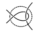

Refer to caption
Refer to caption
Figure 7: Examples of tangle

Let T𝑇T be a tangle in a knot or link projection, then by convention we denote T𝑇-T to be its reflection(or mirror image). For a twist of (n)𝑛(n) crossings proceeding from west to east, we use the twist that is right-handed for n>0𝑛0n>0 and left-handed for n<0𝑛0n<0.

Refer to caption
(a) 333
Refer to caption
(b) 33-3
Figure 8:

Given a tangle T([Uncaptioned image])𝑇[Uncaptioned image]T(\raisebox{-6.00006pt}{\includegraphics[scale={0.4}]{t6.PNG}}), we obtain the numerator, TNsuperscript𝑇𝑁T^{N} by attaching the (top) NW𝑁𝑊NW and NE𝑁𝐸NE edges of T𝑇T together and attaching the (bottom) SW𝑆𝑊SW and SE𝑆𝐸SE edges together. Also the denominator, TDsuperscript𝑇𝐷T^{D} is obtained by attaching the (left side) NW𝑁𝑊NW and SW𝑆𝑊SW edges together and attaching the (right side) NE𝑁𝐸NE and SE𝑆𝐸SE edges together.

Given tangles T([Uncaptioned image])𝑇[Uncaptioned image]T(\raisebox{-6.00006pt}{\includegraphics[scale={0.45}]{t6.PNG}}) and U([Uncaptioned image])𝑈[Uncaptioned image]U(\raisebox{-8.00003pt}{\includegraphics[scale={0.3}]{t59.PNG}}), one defines the sum, denoted T+U𝑇𝑈T+U by placing the diagram for U𝑈U to the right of the diagram for T𝑇T and attaching the NE𝑁𝐸NE edge of T𝑇T to the NW𝑁𝑊NW edge of U𝑈U, and the SE𝑆𝐸SE edge of T𝑇T to the SW𝑆𝑊SW edge of S𝑆S. The resulting tangle T+U𝑇𝑈T+U has exterior edges corresponding to the NW𝑁𝑊NW and SW𝑆𝑊SW edges of T𝑇T and the NE𝑁𝐸NE and SE𝑆𝐸SE edges of U𝑈U. We shall also have occasion to consider the ”vertical sum” of two tangles say T𝑇T and U𝑈U by placing the diagram for U𝑈U below the diagram for T𝑇T and attaching the SE𝑆𝐸SE edge of T𝑇T to the NE𝑁𝐸NE edge of U𝑈U, and the SW𝑆𝑊SW edge of T𝑇T to the NW𝑁𝑊NW edge of U𝑈U. The resulting tangle TU𝑇𝑈T\ast U has exterior edges corresponding to the NW𝑁𝑊NW and NE𝑁𝐸NE edges of T𝑇T and the SW𝑆𝑊SW and SE𝑆𝐸SE edges of U𝑈U.

Refer to caption
Figure 9: Numerator tangle of T𝑇T, TNsuperscript𝑇𝑁T^{N}
Refer to caption
Figure 10: Denominator tangle of T𝑇T, TDsuperscript𝑇𝐷T^{D}
Refer to caption
Figure 11: Tangle T+S𝑇𝑆T+S
Refer to caption
Figure 12: Tangle TS𝑇𝑆T\ast S

We note that the ”integer” tangle n𝑛-n is indeed an additive inverse of the tangle n𝑛n, in that their sum is 0=[Uncaptioned image]0[Uncaptioned image]0=\raisebox{-6.00006pt}{\includegraphics[scale={0.3}]{t21.PNG}}.

We shall denote by T1superscript𝑇1T^{-1}, the reflection of T𝑇T in a NWSE𝑁𝑊𝑆𝐸NW-SE axis. In other words rotating all of it’s edges through 90superscript9090^{\circ} counter-clockwise and finding the mirror image. We define the product of two tangles, T.Uformulae-sequence𝑇𝑈T.U as the tangle sum T1+Usuperscript𝑇1𝑈T^{-1}+U. Note that T.0=T1𝑇.0superscript𝑇1T.0=T^{-1}. Traditionally for n𝑛n\in\mathbb{Z}, n0𝑛0n\neq 0, the tangle n1superscript𝑛1n^{-1} is denoted 1n1𝑛\frac{1}{n} and 01=[Uncaptioned image]superscript01[Uncaptioned image]0^{-1}=\raisebox{-5.0pt}{\includegraphics[scale={0.3}]{t24.PNG}} is denoted \infty.

Refer to caption
(a) 31superscript313^{-1}
Refer to caption
(b) 32323\cdot 2
Figure 13:

Regarding iterated ”product”, we follow the standard convention that TUV𝑇𝑈𝑉T\cdot U\cdot V is to be interpreted as (TU)V𝑇𝑈𝑉(T\cdot U)\cdot V, i.e

TUV𝑇𝑈𝑉\displaystyle T\cdot U\cdot V =\displaystyle= (TU)V𝑇𝑈𝑉\displaystyle(T\cdot U)\cdot V
=\displaystyle= (T1+U)Vsuperscript𝑇1𝑈𝑉\displaystyle(T^{-1}+U)\cdot V
=\displaystyle= [(T1+U)]1+Vsuperscriptdelimited-[]superscript𝑇1𝑈1𝑉\displaystyle[(T^{-1}+U)]^{-1}+V

The class of examples that we consider in this paper are each denoted by H(T,U)𝐻𝑇𝑈H(T,U), where T𝑇T and U𝑈U are each tangles and H(T,U)𝐻𝑇𝑈H(T,U) is a satellite of the Hopf link that conforms to the pattern shown in Figure  14 below.
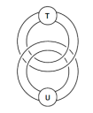
Refer to caption
Figure 14: H(T,U)𝐻𝑇𝑈H(T,U)

4.2 The Bracket Polynomial of H(T,U)𝐻𝑇𝑈H(T,U)

Given a tangle, T𝑇T, the bracket expansion formula; [Uncaptioned image]=A[Uncaptioned image]+A1[Uncaptioned image]delimited-⟨⟩[Uncaptioned image]𝐴delimited-⟨⟩[Uncaptioned image]superscript𝐴1delimited-⟨⟩[Uncaptioned image]\left\langle\raisebox{-8.00003pt}{\includegraphics[scale={0.3}]{t55.PNG}}\right\rangle=A\left\langle\raisebox{-6.00006pt}{\includegraphics[scale={0.3}]{t24.PNG}}\right\rangle+A^{-1}\left\langle\raisebox{-6.00006pt}{\includegraphics[scale={0.3}]{t21.PNG}}\right\rangle together with the rule, LO=δLdelimited-⟨⟩square-union𝐿𝑂𝛿delimited-⟨⟩𝐿\left\langle L\sqcup O\right\rangle=\delta\left\langle L\right\rangle(applicable also to link diagrams) allows us to express the symbol Tdelimited-⟨⟩𝑇\langle T\rangle as a formal linear combination. We have that T=f(T)0+g(T)delimited-⟨⟩𝑇𝑓𝑇delimited-⟨⟩0𝑔𝑇delimited-⟨⟩\langle T\rangle=f(T)\langle 0\rangle+g(T)\langle\infty\rangle, where 0delimited-⟨⟩0\langle 0\rangle,delimited-⟨⟩\langle\infty\rangle are regarded as primitive objects and the coefficient f(T)𝑓𝑇f(T),g(T)𝑔𝑇g(T) are in the ring [A,A1]𝐴superscript𝐴1\mathbb{Z}[A,A^{-1}].

We define the bracket vector of T𝑇T to be the ordered pair (f(T),g(T))𝑓𝑇𝑔𝑇(f(T),g(T)) and denote it by br(T)𝑏𝑟𝑇br(T). For example br(1)=(A,A1)𝑏𝑟1𝐴superscript𝐴1br(1)=(A,A^{-1}). Where appropriate, we shall consider br(T)𝑏𝑟𝑇br(T) as the column vector (f(T)g(T))matrix𝑓𝑇𝑔𝑇\begin{pmatrix}f(T)\\ g(T)\end{pmatrix}.

Example 4.2.

Let us consider the tangle 222 and obtain its bracket vector.

Traditionally we know that the tangle 222 is represented by the diagram, [Uncaptioned image] and we can compute its bracket polynomial as follows,

[Uncaptioned image]delimited-⟨⟩[Uncaptioned image]\displaystyle\left\langle\raisebox{-1.99997pt}{\includegraphics[scale={0.3}]{c1.PNG}}\right\rangle =\displaystyle= A[Uncaptioned image]+A1[Uncaptioned image]𝐴delimited-⟨⟩[Uncaptioned image]superscript𝐴1delimited-⟨⟩[Uncaptioned image]\displaystyle A\left\langle\raisebox{-1.99997pt}{\includegraphics[scale={0.3}]{c4.PNG}}\right\rangle+A^{-1}\left\langle\raisebox{-1.99997pt}{\includegraphics[scale={0.3}]{c3.PNG}}\right\rangle
=\displaystyle= A[A[Uncaptioned image]+A1[Uncaptioned image]]+A1[A[Uncaptioned image]+A1[Uncaptioned image]]𝐴delimited-[]𝐴delimited-⟨⟩[Uncaptioned image]superscript𝐴1delimited-⟨⟩[Uncaptioned image]superscript𝐴1delimited-[]𝐴delimited-⟨⟩[Uncaptioned image]superscript𝐴1delimited-⟨⟩[Uncaptioned image]\displaystyle A\left[A\left\langle\raisebox{-1.99997pt}{\includegraphics[scale={0.3}]{t21.PNG}}\right\rangle+A^{-1}\left\langle\raisebox{-3.99994pt}{\includegraphics[scale={0.3}]{t24.PNG}}\right\rangle\right]+A^{-1}\left[A\left\langle\raisebox{-3.99994pt}{\includegraphics[scale={0.3}]{t24.PNG}}\right\rangle+A^{-1}\left\langle\raisebox{-1.99997pt}{\includegraphics[scale={0.3}]{c2.PNG}}\right\rangle\right]
=\displaystyle= A2[Uncaptioned image]+(2+A2(A2A2))[Uncaptioned image]superscript𝐴2delimited-⟨⟩[Uncaptioned image]2superscript𝐴2superscript𝐴2superscript𝐴2delimited-⟨⟩[Uncaptioned image]\displaystyle A^{2}\left\langle\raisebox{-1.99997pt}{\includegraphics[scale={0.3}]{t21.PNG}}\right\rangle+(2+A^{-2}(-A^{-2}-A^{2}))\left\langle\raisebox{-3.99994pt}{\includegraphics[scale={0.3}]{t24.PNG}}\right\rangle
=\displaystyle= A2[Uncaptioned image]+(2A41)[Uncaptioned image]superscript𝐴2delimited-⟨⟩[Uncaptioned image]2superscript𝐴41delimited-⟨⟩[Uncaptioned image]\displaystyle A^{2}\left\langle\raisebox{-1.99997pt}{\includegraphics[scale={0.3}]{t21.PNG}}\right\rangle+(2-A^{-4}-1)\left\langle\raisebox{-3.99994pt}{\includegraphics[scale={0.3}]{t24.PNG}}\right\rangle
=\displaystyle= A2[Uncaptioned image]+(1A4)[Uncaptioned image]superscript𝐴2delimited-⟨⟩[Uncaptioned image]1superscript𝐴4delimited-⟨⟩[Uncaptioned image]\displaystyle A^{2}\left\langle\raisebox{-1.99997pt}{\includegraphics[scale={0.3}]{t21.PNG}}\right\rangle+(1-A^{-4})\left\langle\raisebox{-3.99994pt}{\includegraphics[scale={0.3}]{t24.PNG}}\right\rangle
=\displaystyle= A20+(1A4)superscript𝐴2delimited-⟨⟩01superscript𝐴4delimited-⟨⟩\displaystyle A^{2}\langle 0\rangle+(1-A^{-4})\langle\infty\rangle

In this example we have that f(T)=A2𝑓𝑇superscript𝐴2f(T)=A^{2} and g(T)=(1A4)𝑔𝑇1superscript𝐴4g(T)=(1-A^{-4}). Our bracket vector is therefore given as br(2)=(A21A4)𝑏𝑟2matrixsuperscript𝐴21superscript𝐴4br(2)=\begin{pmatrix}A^{2}\\ 1-A^{-4}\end{pmatrix}.

Proposition 4.3 ([17]).
  1. 1.

    (TNTD)=(δ11δ)br(T)matrixdelimited-⟨⟩superscript𝑇𝑁delimited-⟨⟩superscript𝑇𝐷matrix𝛿11𝛿𝑏𝑟𝑇\begin{pmatrix}\langle T^{N}\rangle\\ \langle T^{D}\rangle\end{pmatrix}=\begin{pmatrix}\delta&1\\ 1&\delta\end{pmatrix}br(T)

  2. 2.

    br(T+U)=(f(U)0g(U)f(U)+δg(U))br(T).𝑏𝑟𝑇𝑈matrix𝑓𝑈0𝑔𝑈𝑓𝑈𝛿𝑔𝑈𝑏𝑟𝑇br(T+U)=\begin{pmatrix}f(U)&0\\ g(U)&f(U)+\delta g(U)\end{pmatrix}br(T).

    br(TU)=(δf(U)+g(U)f(U)0g(U))br(T).𝑏𝑟𝑇𝑈matrix𝛿𝑓𝑈𝑔𝑈𝑓𝑈0𝑔𝑈𝑏𝑟𝑇br(T\ast U)=\begin{pmatrix}\delta f(U)+g(U)&f(U)\\ 0&g(U)\end{pmatrix}br(T).

Proof.
  1. 1.

    From the above expression of the bracket polynomial of T𝑇T, we know that;

    T=f(T)0+g(T)delimited-⟨⟩𝑇𝑓𝑇delimited-⟨⟩0𝑔𝑇delimited-⟨⟩\langle T\rangle=f(T)\langle 0\rangle+g(T)\langle\infty\rangle, where 0=[Uncaptioned image]0[Uncaptioned image]0=\raisebox{-6.00006pt}{\includegraphics[scale={0.3}]{t21.PNG}}, =[Uncaptioned image][Uncaptioned image]\infty=\raisebox{-6.00006pt}{\includegraphics[scale={0.3}]{t24.PNG}}

    We also note that TN=[Uncaptioned image]superscript𝑇𝑁[Uncaptioned image]T^{N}=\raisebox{-6.00006pt}{\includegraphics[scale={0.3}]{t7.PNG}} and TD=[Uncaptioned image]superscript𝑇𝐷[Uncaptioned image]T^{D}=\raisebox{-5.0pt}{\includegraphics[scale={0.3}]{t8.PNG}}.

    TN=[Uncaptioned image]delimited-⟨⟩superscript𝑇𝑁delimited-⟨⟩[Uncaptioned image]\displaystyle\langle T^{N}\rangle=\left\langle\raisebox{-6.00006pt}{\includegraphics[scale={0.3}]{t7.PNG}}\right\rangle =\displaystyle= f(T)[Uncaptioned image]+g(T)[Uncaptioned image]𝑓𝑇delimited-⟨⟩[Uncaptioned image]𝑔𝑇delimited-⟨⟩[Uncaptioned image]\displaystyle f(T)\left\langle\raisebox{-8.00003pt}{\includegraphics[scale={0.3}]{t20.PNG}}\right\rangle+g(T)\left\langle\raisebox{-8.00003pt}{\includegraphics[scale={0.3}]{t22.PNG}}\right\rangle
    =\displaystyle= δf(T)+g(T)𝛿𝑓𝑇𝑔𝑇\displaystyle\delta f(T)+g(T)

    Also,

    TD=[Uncaptioned image]delimited-⟨⟩superscript𝑇𝐷delimited-⟨⟩[Uncaptioned image]\displaystyle\langle T^{D}\rangle=\left\langle\raisebox{-3.99994pt}{\includegraphics[scale={0.3}]{t8.PNG}}\right\rangle =\displaystyle= f(T)[Uncaptioned image]+g(T)[Uncaptioned image]𝑓𝑇delimited-⟨⟩[Uncaptioned image]𝑔𝑇delimited-⟨⟩[Uncaptioned image]\displaystyle f(T)\left\langle\raisebox{-6.00006pt}{\includegraphics[scale={0.3}]{t23.PNG}}\right\rangle+g(T)\left\langle\raisebox{-6.00006pt}{\includegraphics[scale={0.3}]{t15.PNG}}\right\rangle
    =\displaystyle= f(T)+δg(T)𝑓𝑇𝛿𝑔𝑇\displaystyle f(T)+\delta g(T)

    therefore,

    (TNTD)=(δ11δ)(f(T)g(T))=(δ11δ)br(T)matrixdelimited-⟨⟩superscript𝑇𝑁delimited-⟨⟩superscript𝑇𝐷matrix𝛿11𝛿matrix𝑓𝑇𝑔𝑇matrix𝛿11𝛿𝑏𝑟𝑇\displaystyle\begin{pmatrix}\langle T^{N}\rangle\\ \langle T^{D}\rangle\end{pmatrix}=\begin{pmatrix}\delta&1\\ 1&\delta\end{pmatrix}\begin{pmatrix}f(T)\\ g(T)\end{pmatrix}=\begin{pmatrix}\delta&1\\ 1&\delta\end{pmatrix}br(T)
  2. 2.

    We know that T+U𝑇𝑈T+U is denoted as [Uncaptioned image].

    T+U=[Uncaptioned image]delimited-⟨⟩𝑇𝑈delimited-⟨⟩[Uncaptioned image]\displaystyle\langle T+U\rangle=\left\langle\raisebox{-6.00006pt}{\includegraphics[scale={0.4}]{t9.PNG}}\right\rangle =\displaystyle= f(T)[Uncaptioned image]+g(T)[Uncaptioned image]𝑓𝑇delimited-⟨⟩[Uncaptioned image]𝑔𝑇delimited-⟨⟩[Uncaptioned image]\displaystyle f(T)\left\langle\raisebox{-6.00006pt}{\includegraphics[scale={0.25}]{t17.PNG}}\right\rangle+g(T)\left\langle\raisebox{-6.00006pt}{\includegraphics[scale={0.25}]{t26.PNG}}\right\rangle
    =\displaystyle= f(T)[f(U)[Uncaptioned image]+g(U)[Uncaptioned image]]+g(T)[f(U)[Uncaptioned image]\displaystyle f(T)[f(U)\left\langle\raisebox{-8.00003pt}{\includegraphics[scale={0.25}]{t21.PNG}}\right\rangle+g(U)\left\langle\raisebox{-8.00003pt}{\includegraphics[scale={0.25}]{t24.PNG}}\right\rangle]+g(T)[f(U)\left\langle\raisebox{-8.00003pt}{\includegraphics[scale={0.25}]{t24.PNG}}\right\rangle
    +\displaystyle+ g(U)[Uncaptioned image]]\displaystyle g(U)\left\langle\raisebox{-6.00006pt}{\includegraphics[scale={0.25}]{t18.PNG}}\right\rangle]
    =\displaystyle= f(T)[f(U)[Uncaptioned image]+g(U)[Uncaptioned image]]+g(T)[f(U)[Uncaptioned image]\displaystyle f(T)[f(U)\left\langle\raisebox{-8.00003pt}{\includegraphics[scale={0.25}]{t21.PNG}}\right\rangle+g(U)\left\langle\raisebox{-8.00003pt}{\includegraphics[scale={0.25}]{t24.PNG}}\right\rangle]+g(T)[f(U)\left\langle\raisebox{-8.00003pt}{\includegraphics[scale={0.25}]{t24.PNG}}\right\rangle
    +\displaystyle+ δg(U)[Uncaptioned image]]\displaystyle\delta g(U)\left\langle\raisebox{-8.00003pt}{\includegraphics[scale={0.25}]{t24.PNG}}\right\rangle]
    =\displaystyle= f(T)f(U)[Uncaptioned image]+[f(T)g(U)+g(T)f(U)+δg(T)g(U)][Uncaptioned image]𝑓𝑇𝑓𝑈delimited-⟨⟩[Uncaptioned image]delimited-[]𝑓𝑇𝑔𝑈𝑔𝑇𝑓𝑈𝛿𝑔𝑇𝑔𝑈delimited-⟨⟩[Uncaptioned image]\displaystyle f(T)f(U)\left\langle\raisebox{-8.00003pt}{\includegraphics[scale={0.2}]{t21.PNG}}\right\rangle+[f(T)g(U)+g(T)f(U)+\delta g(T)g(U)]\left\langle\raisebox{-8.00003pt}{\includegraphics[scale={0.2}]{t24.PNG}}\right\rangle

    f(T+U)=f(T)f(U)absent𝑓𝑇𝑈𝑓𝑇𝑓𝑈\Longrightarrow f(T+U)=f(T)f(U) and g(T+U)=f(T)g(U)+g(T)f(U)+δg(T)g(U)𝑔𝑇𝑈𝑓𝑇𝑔𝑈𝑔𝑇𝑓𝑈𝛿𝑔𝑇𝑔𝑈g(T+U)=f(T)g(U)+g(T)f(U)+\delta g(T)g(U)

    therefore,

    br(T+U)=(f(T)f(U)f(T)g(U)+g(T)f(U)+δg(T)g(U))𝑏𝑟𝑇𝑈matrix𝑓𝑇𝑓𝑈𝑓𝑇𝑔𝑈𝑔𝑇𝑓𝑈𝛿𝑔𝑇𝑔𝑈\displaystyle br(T+U)=\begin{pmatrix}f(T)f(U)\\ f(T)g(U)+g(T)f(U)+\delta g(T)g(U)\end{pmatrix} =\displaystyle= (f(U)0g(U)f(U)+δg(U))(f(T)g(T))matrix𝑓𝑈0𝑔𝑈𝑓𝑈𝛿𝑔𝑈matrix𝑓𝑇𝑔𝑇\displaystyle\begin{pmatrix}f(U)&0\\ g(U)&f(U)+\delta g(U)\end{pmatrix}\begin{pmatrix}f(T)\\ g(T)\end{pmatrix}
    =\displaystyle= (f(U)0g(U)f(U)+δg(U))br(T)matrix𝑓𝑈0𝑔𝑈𝑓𝑈𝛿𝑔𝑈𝑏𝑟𝑇\displaystyle\begin{pmatrix}f(U)&0\\ g(U)&f(U)+\delta g(U)\end{pmatrix}br(T)

    Also, we know that TU𝑇𝑈T\ast U is denoted as [Uncaptioned image]

    TU=[Uncaptioned image]delimited-⟨⟩𝑇𝑈delimited-⟨⟩[Uncaptioned image]\displaystyle\langle T\ast U\rangle=\left\langle\raisebox{-11.99998pt}{\includegraphics[scale={0.4}]{t10.PNG}}\right\rangle =\displaystyle= f(T)[Uncaptioned image]+g(T)[Uncaptioned image]𝑓𝑇delimited-⟨⟩[Uncaptioned image]𝑔𝑇delimited-⟨⟩[Uncaptioned image]\displaystyle f(T)\left\langle\raisebox{-13.99995pt}{\includegraphics[scale={0.2}]{t28.PNG}}\right\rangle+g(T)\left\langle\raisebox{-11.99998pt}{\includegraphics[scale={0.25}]{t27.PNG}}\right\rangle
    =\displaystyle= f(T)[f(U)[Uncaptioned image]+g(U)[Uncaptioned image]]+g(T)[f(U)[Uncaptioned image]\displaystyle f(T)[f(U)\left\langle\raisebox{-16.00008pt}{\includegraphics[scale={0.25}]{t19.PNG}}\right\rangle+g(U)\left\langle\raisebox{-8.00003pt}{\includegraphics[scale={0.25}]{t21.PNG}}\right\rangle]+g(T)[f(U)\left\langle\raisebox{-8.00003pt}{\includegraphics[scale={0.25}]{t21.PNG}}\right\rangle
    +\displaystyle+ g(U)[Uncaptioned image]]\displaystyle g(U)\left\langle\raisebox{-8.00003pt}{\includegraphics[scale={0.25}]{t24.PNG}}\right\rangle]
    =\displaystyle= f(T)[δf(U)[Uncaptioned image]+g(U)[Uncaptioned image]]+g(T)[f(U)[Uncaptioned image]\displaystyle f(T)[\delta f(U)\left\langle\raisebox{-8.00003pt}{\includegraphics[scale={0.25}]{t21.PNG}}\right\rangle+g(U)\left\langle\raisebox{-8.00003pt}{\includegraphics[scale={0.25}]{t21.PNG}}\right\rangle]+g(T)[f(U)\left\langle\raisebox{-8.00003pt}{\includegraphics[scale={0.25}]{t21.PNG}}\right\rangle
    +\displaystyle+ g(U)[Uncaptioned image]]\displaystyle g(U)\left\langle\raisebox{-8.00003pt}{\includegraphics[scale={0.25}]{t24.PNG}}\right\rangle]
    =\displaystyle= [δf(T)f(U)+f(T)g(U)+g(T)f(U)][Uncaptioned image]+g(T)g(U)[Uncaptioned image]delimited-[]𝛿𝑓𝑇𝑓𝑈𝑓𝑇𝑔𝑈𝑔𝑇𝑓𝑈delimited-⟨⟩[Uncaptioned image]𝑔𝑇𝑔𝑈delimited-⟨⟩[Uncaptioned image]\displaystyle[\delta f(T)f(U)+f(T)g(U)+g(T)f(U)]\left\langle\raisebox{-8.00003pt}{\includegraphics[scale={0.25}]{t21.PNG}}\right\rangle+g(T)g(U)\left\langle\raisebox{-8.00003pt}{\includegraphics[scale={0.25}]{t24.PNG}}\right\rangle

    f(TU)=δf(T)f(U)+f(T)g(U)+g(T)f(U)absent𝑓𝑇𝑈𝛿𝑓𝑇𝑓𝑈𝑓𝑇𝑔𝑈𝑔𝑇𝑓𝑈\Longrightarrow f(T\ast U)=\delta f(T)f(U)+f(T)g(U)+g(T)f(U) and g(TU)=g(T)g(U))g(T\ast U)=g(T)g(U))

    therefore,

    br(TU)=(δf(T)f(U)+f(T)g(U)+g(T)f(U)g(T)g(U))𝑏𝑟𝑇𝑈matrix𝛿𝑓𝑇𝑓𝑈𝑓𝑇𝑔𝑈𝑔𝑇𝑓𝑈𝑔𝑇𝑔𝑈\displaystyle br(T\ast U)=\begin{pmatrix}\delta f(T)f(U)+f(T)g(U)+g(T)f(U)\\ g(T)g(U)\end{pmatrix} =\displaystyle= (δf(U)+g(U)f(U)0g(U))(f(T)g(T))matrix𝛿𝑓𝑈𝑔𝑈𝑓𝑈0𝑔𝑈matrix𝑓𝑇𝑔𝑇\displaystyle\begin{pmatrix}\delta f(U)+g(U)&f(U)\\ 0&g(U)\end{pmatrix}\begin{pmatrix}f(T)\\ g(T)\end{pmatrix}
    =\displaystyle= (δf(U)+g(U)f(U)0g(U))br(T)matrix𝛿𝑓𝑈𝑔𝑈𝑓𝑈0𝑔𝑈𝑏𝑟𝑇\displaystyle\begin{pmatrix}\delta f(U)+g(U)&f(U)\\ 0&g(U)\end{pmatrix}br(T)

Now considering the class of link under study,H(T,U)𝐻𝑇𝑈H(T,U). We observe that if we take (T,U)=(0,0)𝑇𝑈00(T,U)=(0,0) we obtain the 222-strand parallel of the standard diagram of the Hopf link. The bracket polynomial of that diagram was computed in Example  3.5 of the previous chapter to be;

(A14+A6+2A2+2A2+A6+A14)superscript𝐴14superscript𝐴62superscript𝐴22superscript𝐴2superscript𝐴6superscript𝐴14-(A^{-14}+A^{-6}+2A^{-2}+2A^{2}+A^{6}+A^{14})

The choice (T,U)=(0,)𝑇𝑈0(T,U)=(0,\infty)(or (T,U)=(,0)𝑇𝑈0(T,U)=(\infty,0)) yields a diagram with writhe 0 of the unlink with 333 components and (T,U)=(,)𝑇𝑈(T,U)=(\infty,\infty) gives a diagram with writhe 0 of the unlink with 222 components. Therefore the bracket polynomial of H(0,)𝐻0H(0,\infty), H(,)𝐻H(\infty,\infty) are δ2superscript𝛿2\delta^{2},δ𝛿\delta respectively.

Let us define;

h00=H(0,0)=(A14+A6+2A2+2A2+A6+A14)subscript00delimited-⟨⟩𝐻00superscript𝐴14superscript𝐴62superscript𝐴22superscript𝐴2superscript𝐴6superscript𝐴14h_{00}=\langle H(0,0)\rangle=-(A^{-14}+A^{-6}+2A^{-2}+2A^{2}+A^{6}+A^{14}) (19)
h01=h10=H(0,)=δ2subscript01subscript10delimited-⟨⟩𝐻0superscript𝛿2h_{01}=h_{10}=\langle H(0,\infty)\rangle=\delta^{2} (20)
h11=H(,)=δsubscript11delimited-⟨⟩𝐻𝛿h_{11}=\langle H(\infty,\infty)\rangle=\delta (21)

and let \mathcal{M} denote the matrix, (h00h01h10h11)matrixsubscript00subscript01subscript10subscript11\begin{pmatrix}h_{00}&h_{01}\\ h_{10}&h_{11}\end{pmatrix}

Proposition 4.4 ([17]).

H(T,U)=h00f(T)f(U)+h01[f(T)g(U)+g(T)f(U)]+h11g(T)g(U)delimited-⟨⟩𝐻𝑇𝑈subscript00𝑓𝑇𝑓𝑈subscript01delimited-[]𝑓𝑇𝑔𝑈𝑔𝑇𝑓𝑈subscript11𝑔𝑇𝑔𝑈\langle H(T,U)\rangle=h_{00}f(T)f(U)+h_{01}[f(T)g(U)+g(T)f(U)]+h_{11}g(T)g(U)

or in the matrix notation,

H(T,U)=br(T)tbr(U)delimited-⟨⟩𝐻𝑇𝑈𝑏𝑟superscript𝑇𝑡𝑏𝑟𝑈\langle H(T,U)\rangle=br(T)^{t}\cdot\mathcal{M}\cdot br(U)

Proof.
H(T,U)delimited-⟨⟩𝐻𝑇𝑈\displaystyle\langle H(T,U)\rangle =\displaystyle= [Uncaptioned image]delimited-⟨⟩[Uncaptioned image]\displaystyle\left\langle\raisebox{-15.00002pt}{\includegraphics[scale={0.25}]{t54.PNG}}\right\rangle
=\displaystyle= f(T)[Uncaptioned image]+g(T)[Uncaptioned image]𝑓𝑇delimited-⟨⟩[Uncaptioned image]𝑔𝑇delimited-⟨⟩[Uncaptioned image]\displaystyle f(T)\left\langle\raisebox{-16.00008pt}{\includegraphics[scale={0.25}]{t33.PNG}}\right\rangle+g(T)\left\langle\raisebox{-16.00008pt}{\includegraphics[scale={0.25}]{t29.PNG}}\right\rangle
=\displaystyle= f(T)[f(U)[Uncaptioned image]+g(U)[Uncaptioned image]]+g(T)[f(U)[Uncaptioned image]+g(U)[Uncaptioned image]]𝑓𝑇delimited-[]𝑓𝑈delimited-⟨⟩[Uncaptioned image]𝑔𝑈delimited-⟨⟩[Uncaptioned image]𝑔𝑇delimited-[]𝑓𝑈delimited-⟨⟩[Uncaptioned image]𝑔𝑈delimited-⟨⟩[Uncaptioned image]\displaystyle f(T)\left[f(U)\left\langle\raisebox{-16.00008pt}{\includegraphics[scale={0.25}]{t34.PNG}}\right\rangle+g(U)\left\langle\raisebox{-16.00008pt}{\includegraphics[scale={0.25}]{t31.PNG}}\right\rangle\right]+g(T)\left[f(U)\left\langle\raisebox{-16.00008pt}{\includegraphics[scale={0.25}]{t32.PNG}}\right\rangle+g(U)\left\langle\raisebox{-16.00008pt}{\includegraphics[scale={0.25}]{t30.PNG}}\right\rangle\right]
=\displaystyle= f(T)f(U)H(0,0)+f(T)g(U)H(0,)+g(T)f(U)H(,0)+g(T)g(U)H(,)𝑓𝑇𝑓𝑈delimited-⟨⟩𝐻00𝑓𝑇𝑔𝑈delimited-⟨⟩𝐻0𝑔𝑇𝑓𝑈delimited-⟨⟩𝐻0𝑔𝑇𝑔𝑈delimited-⟨⟩𝐻\displaystyle f(T)f(U)\langle H(0,0)\rangle+f(T)g(U)\langle H(0,\infty)\rangle+g(T)f(U)\langle H(\infty,0)\rangle+g(T)g(U)\langle H(\infty,\infty)\rangle
=\displaystyle= h00f(T)f(U)+h01[f(T)g(U)+g(T)f(U)]+h11g(T)g(U)subscript00𝑓𝑇𝑓𝑈subscript01delimited-[]𝑓𝑇𝑔𝑈𝑔𝑇𝑓𝑈subscript11𝑔𝑇𝑔𝑈\displaystyle h_{00}f(T)f(U)+h_{01}[f(T)g(U)+g(T)f(U)]+h_{11}g(T)g(U)

We can now check that br(T)tbr(U)=h00f(T)f(U)+h01(f(T)g(U)+g(T)f(U))+h11g(T)g(U)𝑏𝑟superscript𝑇𝑡𝑏𝑟𝑈subscript00𝑓𝑇𝑓𝑈subscript01𝑓𝑇𝑔𝑈𝑔𝑇𝑓𝑈subscript11𝑔𝑇𝑔𝑈br(T)^{t}\cdot\mathcal{M}\cdot br(U)=h_{00}f(T)f(U)+h_{01}(f(T)g(U)+g(T)f(U))+h_{11}g(T)g(U)

br(T)tbr(U)𝑏𝑟superscript𝑇𝑡𝑏𝑟𝑈\displaystyle br(T)^{t}\cdot\mathcal{M}\cdot br(U) =\displaystyle= br(T)t(br(U))𝑏𝑟superscript𝑇𝑡𝑏𝑟𝑈\displaystyle br(T)^{t}\cdot(\mathcal{M}\cdot br(U))
=\displaystyle= br(T)t[(h00h01h10h11)(f(U)g(U))]𝑏𝑟superscript𝑇𝑡delimited-[]matrixsubscript00subscript01subscript10subscript11matrix𝑓𝑈𝑔𝑈\displaystyle br(T)^{t}\cdot\left[\begin{pmatrix}h_{00}&h_{01}\\ h_{10}&h_{11}\end{pmatrix}\cdot\begin{pmatrix}f(U)\\ g(U)\end{pmatrix}\right]
=\displaystyle= (f(T)g(T))(h00f(U)+h01g(U)h10f(U)+h11g(U))matrix𝑓𝑇𝑔𝑇matrixsubscript00𝑓𝑈subscript01𝑔𝑈subscript10𝑓𝑈subscript11𝑔𝑈\displaystyle\begin{pmatrix}f(T)&g(T)\end{pmatrix}\cdot\begin{pmatrix}h_{00}f(U)+h_{01}g(U)\\ h_{10}f(U)+h_{11}g(U)\end{pmatrix}
=\displaystyle= f(T)[h00f(U)+h01g(U)]+g(T)[h10f(U)+h11g(U)]𝑓𝑇delimited-[]subscript00𝑓𝑈subscript01𝑔𝑈𝑔𝑇delimited-[]subscript10𝑓𝑈subscript11𝑔𝑈\displaystyle f(T)[h_{00}f(U)+h_{01}g(U)]+g(T)[h_{10}f(U)+h_{11}g(U)]
=\displaystyle= h00f(T)f(U)+h01[f(T)g(U)+g(T)f(U)]+h11g(T)g(U)subscript00𝑓𝑇𝑓𝑈subscript01delimited-[]𝑓𝑇𝑔𝑈𝑔𝑇𝑓𝑈subscript11𝑔𝑇𝑔𝑈\displaystyle h_{00}f(T)f(U)+h_{01}[f(T)g(U)+g(T)f(U)]+h_{11}g(T)g(U)

5 The Present Status of Links with Trivial Jones Polynomial

5.1 The Omega Operation.

We apply a method based on the transformation H(T,U)H(T,U)ω𝐻𝑇𝑈𝐻superscript𝑇𝑈𝜔H(T,U)\longrightarrow H(T,U)^{\omega} to construct links with trivial Jones polynomial. In this transformation, tangles T𝑇T and U𝑈U are cut out and re-glued by certain specific homeomorphisms of the tangle boundaries. The transformation ω𝜔\omega has a property of preserving the Kauffman bracket polynomial. It is however, effective in generating examples, as a trivial link can be transformed to a prime link and repeated application yields an infinite sequence of inequivalent links.

Definition 5.1 ([17]).

Given a tangle T𝑇T, Tωsuperscript𝑇𝜔T^{\omega} denotes the tangle (T+2).1.2𝑇2.1.2(T+2).1.2 and Tω¯superscript𝑇¯𝜔T^{\bar{\omega}} the tangle (T2).(1).(2)formulae-sequence𝑇212(T-2).(-1).(-2).

Refer to caption
Refer to caption
Figure 15: Tωsuperscript𝑇𝜔T^{\omega} and Tω¯superscript𝑇¯𝜔T^{\bar{\omega}}

Using the ”vertical sum” operation introduced in chapter 333, we can as well write,

Tω=((T+2)1)+2superscript𝑇𝜔𝑇212T^{\omega}=((T+2)*1)+2 (22)
Tω¯=((T2)(1))2superscript𝑇¯𝜔𝑇212T^{\bar{\omega}}=((T-2)*(-1))-2 (23)

At this point we determine the effect that the operation ω𝜔\omega and ω¯¯𝜔\bar{\omega} have on bracket vector of a tangle.

From Proposition  4.3 222 we have,

br(T+1)𝑏𝑟𝑇1\displaystyle br(T+1) =\displaystyle= (A0A1A+δA1)br(T),whereδ=A2A2matrix𝐴0superscript𝐴1𝐴𝛿superscript𝐴1𝑏𝑟𝑇where𝛿superscript𝐴2superscript𝐴2\displaystyle\begin{pmatrix}A&0\\ A^{-1}&A+\delta A^{-1}\end{pmatrix}br(T),\qquad\text{where}\quad\delta=-A^{2}-A^{-2}
=\displaystyle= (A0A1A3)br(T)matrix𝐴0superscript𝐴1superscript𝐴3𝑏𝑟𝑇\displaystyle\begin{pmatrix}A&0\\ A^{-1}&-A^{-3}\end{pmatrix}br(T)

and

br(T1)𝑏𝑟𝑇1\displaystyle br(T*1) =\displaystyle= (δA+A1A0A1)br(T),whereδ=A2A2matrix𝛿𝐴superscript𝐴1𝐴0superscript𝐴1𝑏𝑟𝑇where𝛿superscript𝐴2superscript𝐴2\displaystyle\begin{pmatrix}\delta A+A^{-1}&A\\ 0&A^{-1}\end{pmatrix}br(T),\qquad\text{where}\quad\delta=-A^{2}-A^{-2}
=\displaystyle= (A3A0A1)br(T)matrixsuperscript𝐴3𝐴0superscript𝐴1𝑏𝑟𝑇\displaystyle\begin{pmatrix}-A^{3}&A\\ 0&A^{-1}\end{pmatrix}br(T)

Similarly we have that,

br(T+(1))=M+1br(T)𝑏𝑟𝑇1superscriptsubscript𝑀1𝑏𝑟𝑇br(T+(-1))=M_{+}^{-1}\cdot br(T) (24)
br(T(1))=M1br(T)𝑏𝑟𝑇1superscriptsubscript𝑀1𝑏𝑟𝑇br(T*(-1))=M_{*}^{-1}\cdot br(T) (25)

where

M+=(A0A1A3)subscript𝑀matrix𝐴0superscript𝐴1superscript𝐴3M_{+}=\begin{pmatrix}A&0\\ A^{-1}&-A^{-3}\end{pmatrix} ,  M=(A3A0A1)subscript𝑀matrixsuperscript𝐴3𝐴0superscript𝐴1M_{*}=\begin{pmatrix}-A^{3}&A\\ 0&A^{-1}\end{pmatrix}

In this context it is natural to introduce the 2×2222\times 2 matrix,

Ω=M+2MM+2=(A1+A3A7A3A11+2A72A3+2AA5A13A9+A5)Ωsuperscriptsubscript𝑀2subscript𝑀superscriptsubscript𝑀2matrixsuperscript𝐴1superscript𝐴3superscript𝐴7superscript𝐴3superscript𝐴112superscript𝐴72superscript𝐴32𝐴superscript𝐴5superscript𝐴13superscript𝐴9superscript𝐴5\Omega=M_{+}^{2}M_{*}M_{+}^{2}=\begin{pmatrix}-A^{-1}+A^{3}-A^{7}&A^{-3}\\ -A^{-11}+2A^{-7}-2A^{-3}+2A-A^{5}&A^{-13}-A^{-9}+A^{-5}\end{pmatrix} (26)
Proposition 5.2 ([17]).
  1. 1.

    br(Tω)=Ωbr(T)𝑏𝑟superscript𝑇𝜔Ω𝑏𝑟𝑇br(T^{\omega})=\Omega\cdot br(T)

  2. 2.

    br(Tω¯)=Ω1br(T)𝑏𝑟superscript𝑇¯𝜔superscriptΩ1𝑏𝑟𝑇br(T^{\bar{\omega}})=\Omega^{-1}\cdot br(T)

Proof.
br(Tω)𝑏𝑟superscript𝑇𝜔\displaystyle br(T^{\omega}) =\displaystyle= br(((T+2)1)+2)𝑏𝑟𝑇212\displaystyle br(((T+2)*1)+2)
=\displaystyle= M+br(((T+2)1)+1)subscript𝑀𝑏𝑟𝑇211\displaystyle M_{+}\cdot br(((T+2)*1)+1)
=\displaystyle= M+2br((T+2)1)superscriptsubscript𝑀2𝑏𝑟𝑇21\displaystyle M_{+}^{2}\cdot br((T+2)*1)
=\displaystyle= M+2Mbr(T+2)superscriptsubscript𝑀2subscript𝑀𝑏𝑟𝑇2\displaystyle M_{+}^{2}M_{*}\cdot br(T+2)
=\displaystyle= M+2MM+br(T+1)superscriptsubscript𝑀2subscript𝑀subscript𝑀𝑏𝑟𝑇1\displaystyle M_{+}^{2}M_{*}M_{+}\cdot br(T+1)
=\displaystyle= M+2MM+2br(T)superscriptsubscript𝑀2subscript𝑀superscriptsubscript𝑀2𝑏𝑟𝑇\displaystyle M_{+}^{2}M_{*}M_{+}^{2}\cdot br(T)
=\displaystyle= Ωbr(T)Ω𝑏𝑟𝑇\displaystyle\Omega\cdot br(T)
br(Tω¯)𝑏𝑟superscript𝑇¯𝜔\displaystyle br(T^{\bar{\omega}}) =\displaystyle= br(((T2)(1))2)𝑏𝑟𝑇212\displaystyle br(((T-2)*(-1))-2)
=\displaystyle= M+1br(((T2)(1))1)superscriptsubscript𝑀1𝑏𝑟𝑇211\displaystyle M_{+}^{-1}\cdot br(((T-2)*(-1))-1)
=\displaystyle= M+2br((T2)(1))superscriptsubscript𝑀2𝑏𝑟𝑇21\displaystyle M_{+}^{-2}\cdot br((T-2)*(-1))
=\displaystyle= M+2M1br(T2)superscriptsubscript𝑀2superscriptsubscript𝑀1𝑏𝑟𝑇2\displaystyle M_{+}^{-2}M_{*}^{-1}\cdot br(T-2)
=\displaystyle= M+2M1M+1br(T1)superscriptsubscript𝑀2superscriptsubscript𝑀1superscriptsubscript𝑀1𝑏𝑟𝑇1\displaystyle M_{+}^{-2}M_{*}^{-1}M_{+}^{-1}\cdot br(T-1)
=\displaystyle= M+2M1M+2br(T)superscriptsubscript𝑀2superscriptsubscript𝑀1superscriptsubscript𝑀2𝑏𝑟𝑇\displaystyle M_{+}^{-2}M_{*}^{-1}M_{+}^{-2}\cdot br(T)
=\displaystyle= Ω1br(T)superscriptΩ1𝑏𝑟𝑇\displaystyle\Omega^{-1}\cdot br(T)

Definition 5.3 ([17]).

Given tangles T𝑇T,U𝑈U, H(T,U)ω𝐻superscript𝑇𝑈𝜔H(T,U)^{\omega} denotes the diagram H(Tω,Uω¯)𝐻superscript𝑇𝜔superscript𝑈¯𝜔H(T^{\omega},U^{\bar{\omega}})(i.e H(T,U)ω=H(Tω,Uω¯)𝐻superscript𝑇𝑈𝜔𝐻superscript𝑇𝜔superscript𝑈¯𝜔H(T,U)^{\omega}=H(T^{\omega},U^{\bar{\omega}})).

In this context we designate H(T,U)ω=H(Tω,Uω¯)𝐻superscript𝑇𝑈𝜔𝐻superscript𝑇𝜔superscript𝑈¯𝜔H(T,U)^{\omega}=H(T^{\omega},U^{\bar{\omega}}) as the diagram obtained by replacing T𝑇T by Tωsuperscript𝑇𝜔T^{\omega} and U𝑈U by Uω¯superscript𝑈¯𝜔U^{\bar{\omega}}.

Theorem 5.4 ([17]).

Let T𝑇T, U𝑈U be any tangles. Then the bracket polynomials of H(T,U)𝐻𝑇𝑈H(T,U) and H(T,U)ω𝐻superscript𝑇𝑈𝜔H(T,U)^{\omega} are equal.

Proof.
H(Tω,Uω¯)delimited-⟨⟩𝐻superscript𝑇𝜔superscript𝑈¯𝜔\displaystyle\langle H(T^{\omega},U^{\bar{\omega}})\rangle =\displaystyle= br(Tω)tbr(Uω¯)𝑏𝑟superscriptsuperscript𝑇𝜔𝑡𝑏𝑟superscript𝑈¯𝜔\displaystyle br(T^{\omega})^{t}\cdot\mathcal{M}\cdot br(U^{\bar{\omega}})
=\displaystyle= (Ωbr(T))tΩ1br(U)superscriptΩ𝑏𝑟𝑇𝑡superscriptΩ1𝑏𝑟𝑈\displaystyle(\Omega\cdot br(T))^{t}\cdot\mathcal{M}\cdot\Omega^{-1}\cdot br(U)
=\displaystyle= (br(T))tΩtΩ1br(U)superscript𝑏𝑟𝑇𝑡superscriptΩ𝑡superscriptΩ1𝑏𝑟𝑈\displaystyle(br(T))^{t}\cdot\Omega^{t}\cdot\mathcal{M}\cdot\Omega^{-1}\cdot br(U)

We now need to verify that ΩtΩ1=superscriptΩ𝑡superscriptΩ1\Omega^{t}\cdot\mathcal{M}\cdot\Omega^{-1}=\mathcal{M}, where

=((A14+A6+2A2+2A2+A6+A14)A4+A4+2A4+A4+2A2A2)matrixsuperscript𝐴14superscript𝐴62superscript𝐴22superscript𝐴2superscript𝐴6superscript𝐴14superscript𝐴4superscript𝐴42superscript𝐴4superscript𝐴42superscript𝐴2superscript𝐴2\mathcal{M}=\begin{pmatrix}-(A^{-14}+A^{-6}+2A^{-2}+2A^{2}+A^{6}+A^{14})&A^{-4}+A^{4}+2\\ A^{-4}+A^{4}+2&-A^{-2}-A^{2}\end{pmatrix} (27)

Considering the matrix ΩΩ\Omega in Equation  (26)

Ωt=(A1+A3A7A11+2A72A3+2AA5A3A13A9+A5)superscriptΩ𝑡matrixsuperscript𝐴1superscript𝐴3superscript𝐴7superscript𝐴112superscript𝐴72superscript𝐴32𝐴superscript𝐴5superscript𝐴3superscript𝐴13superscript𝐴9superscript𝐴5\displaystyle\Omega^{t}=\begin{pmatrix}-A^{-1}+A^{3}-A^{7}&-A^{-11}+2A^{-7}-2A^{-3}+2A-A^{5}\\ A^{-3}&A^{-13}-A^{-9}+A^{-5}\end{pmatrix}
Ω1superscriptΩ1\displaystyle\Omega^{-1} =\displaystyle= 1A6(A13A9+A5A3A112A7+2A32A+A5A1+A3A7)1superscript𝐴6matrixsuperscript𝐴13superscript𝐴9superscript𝐴5superscript𝐴3superscript𝐴112superscript𝐴72superscript𝐴32𝐴superscript𝐴5superscript𝐴1superscript𝐴3superscript𝐴7\displaystyle-\frac{1}{A^{-6}}\begin{pmatrix}A^{-13}-A^{-9}+A^{-5}&-A^{-3}\\ A^{-11}-2A^{-7}+2A^{-3}-2A+A^{5}&-A^{-1}+A^{3}-A^{7}\end{pmatrix}
=\displaystyle= (A7+A3A1A3A5+2A12A3+2A7A11A5A9+A13)matrixsuperscript𝐴7superscript𝐴3superscript𝐴1superscript𝐴3superscript𝐴52superscript𝐴12superscript𝐴32superscript𝐴7superscript𝐴11superscript𝐴5superscript𝐴9superscript𝐴13\displaystyle\begin{pmatrix}-A^{-7}+A^{-3}-A^{1}&A^{3}\\ -A^{-5}+2A^{-1}-2A^{3}+2A^{7}-A^{11}&A^{5}-A^{9}+A^{13}\end{pmatrix}

Now by direct matrix multiplication we have that,

Ωt=(A11+3A7+A3+2A+A5+2A13A17+A21A13A9A5A1A3A11A13A9A5A1A3A11A15+A7+A3+A)superscriptΩ𝑡matrixsuperscript𝐴113superscript𝐴7superscript𝐴32𝐴superscript𝐴52superscript𝐴13superscript𝐴17superscript𝐴21superscript𝐴13superscript𝐴9superscript𝐴5superscript𝐴1superscript𝐴3superscript𝐴11superscript𝐴13superscript𝐴9superscript𝐴5superscript𝐴1superscript𝐴3superscript𝐴11superscript𝐴15superscript𝐴7superscript𝐴3𝐴\Omega^{t}\cdot\mathcal{M}=\begin{pmatrix}-A^{-11}+3A^{-7}+A^{-3}+2A+A^{5}+2A^{13}-A^{17}+A^{21}&A^{-13}-A^{-9}-A^{-5}-A^{-1}-A^{3}-A^{11}\\ A^{-13}-A^{-9}-A^{-5}-A^{-1}-A^{3}-A^{11}&-A^{-15}+A^{-7}+A^{-3}+A\end{pmatrix} (28)

We therefore have that,

(Ωt)Ω1=((A14+A6+2A2+2A2+A6+A14)A4+A4+2A4+A4+2A2A2)=superscriptΩ𝑡superscriptΩ1matrixsuperscript𝐴14superscript𝐴62superscript𝐴22superscript𝐴2superscript𝐴6superscript𝐴14superscript𝐴4superscript𝐴42superscript𝐴4superscript𝐴42superscript𝐴2superscript𝐴2(\Omega^{t}\cdot\mathcal{M})\cdot\Omega^{-1}=\begin{pmatrix}-(A^{-14}+A^{-6}+2A^{-2}+2A^{2}+A^{6}+A^{14})&A^{-4}+A^{4}+2\\ A^{-4}+A^{4}+2&-A^{-2}-A^{2}\end{pmatrix}=\mathcal{M} (29)

and hence

H(Tω,Uω¯)delimited-⟨⟩𝐻superscript𝑇𝜔superscript𝑈¯𝜔\displaystyle\langle H(T^{\omega},U^{\bar{\omega}})\rangle =\displaystyle= (br(T))tΩtΩ1br(U)superscript𝑏𝑟𝑇𝑡superscriptΩ𝑡superscriptΩ1𝑏𝑟𝑈\displaystyle(br(T))^{t}\cdot\Omega^{t}\cdot\mathcal{M}\cdot\Omega^{-1}\cdot br(U)
=\displaystyle= (br(T))tbr(U)superscript𝑏𝑟𝑇𝑡𝑏𝑟𝑈\displaystyle(br(T))^{t}\cdot\mathcal{M}\cdot br(U)
=\displaystyle= H(T,U)delimited-⟨⟩𝐻𝑇𝑈\displaystyle\langle H(T,U)\rangle

5.2 Thistlethwaite’s Example

The figure  16 below is a version of a link discovered by Morwen Thistlethwaite [14] in December 200020002000. This is an example of a link which is linked but whose linking cannot be detected by the Jones polynomial.This fact can be verified using a computer program or a polynomial invariant like the Kauffman polynomial.
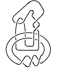
Refer to caption
Figure 16: Thistlethwaite’s link

It interesting to note that we can verify that the Thistlethwaite’s link fits into the structure we consider in this paper. This can be done by choosing tangle T𝑇T as 11-1 and tangle U𝑈U as +22\infty+2 resulting in the figure  17 below with writhe 33-3.

Refer to caption
Figure 17: Unlink with writhe 33-3

We perform the omega transformation on the tangles T𝑇T and U𝑈U and make use of regular isotopy as shown in  (30) and  (31).

[Uncaptioned image]𝜔[Uncaptioned image]=[Uncaptioned image]superscript[Uncaptioned image]𝜔[Uncaptioned image]=[Uncaptioned image]\includegraphics[scale={0.2}]{a4.PNG}^{\qquad\xrightarrow{\huge{\omega}}}\qquad\includegraphics[scale={0.2}]{a7.PNG}\qquad\raisebox{18.99995pt}{=}\includegraphics[scale={0.25}]{a5.PNG} (30)

and

[Uncaptioned image]ω¯[Uncaptioned image]=[Uncaptioned image]superscript[Uncaptioned image]¯𝜔[Uncaptioned image]=[Uncaptioned image]\includegraphics[scale={0.3}]{z5.PNG}^{\qquad\xrightarrow{\huge{\bar{\omega}}}}\qquad\includegraphics[scale={0.2}]{z6.PNG}\qquad\raisebox{18.99995pt}{=}\includegraphics[scale={0.3}]{z3.PNG} (31)

We therefore obtain the Thistlethwaite’s link, figure  16 by replacing the new tangles in figure  17. It is not difficult to see that the writhe of the Thistlethwaite’s link is 33-3. This shows how the first example of Thistlethwaite fits the construction.

5.3 A family of 2-component link with trivial Jones polynomial

In this section we consider a sequence of 2-component links generated by T=2𝑇2T=\infty-2 and U=T=+2𝑈𝑇2U=-T=\infty+2. The diagram H(2,+2)𝐻22H(\infty-2,\infty+2) in figure  18 is a 2-component link of writhe 00; therefore a repeated application of the omega operation on the tangle T=2𝑇2T=\infty-2 yields a sequence of tangles T0=2subscript𝑇02T_{0}=\infty-2 T1=3subscript𝑇13T_{1}=3, T2=512subscript𝑇2512T_{2}=5\cdot 1\cdot 2, T3=51412subscript𝑇351412T_{3}=5\cdot 1\cdot 4\cdot 1\cdot 2,… such that H(Tn,Tn)=δdelimited-⟨⟩𝐻subscript𝑇𝑛subscript𝑇𝑛𝛿\langle H(T_{n},-T_{n})\rangle=\delta for all n0𝑛0n\geq 0.

Refer to caption
Figure 18: H(2,+2)𝐻22H(\infty-2,\infty+2)
Definition 5.5.

S(n)=H(Tn,Tn)𝑆𝑛𝐻subscript𝑇𝑛subscript𝑇𝑛S(n)=H(T_{n},-T_{n}), where the tangle Tnsubscript𝑇𝑛T_{n} is the result of n𝑛n applications of the omega operation.

It is easy to verify that the writhe of H(Tn,Tn)𝐻subscript𝑇𝑛subscript𝑇𝑛H(T_{n},-T_{n}) is zero for even n𝑛n and for odd n𝑛n the writhe is ±8plus-or-minus8\pm 8, the sign depends on the choice of orientation.

Theorem 5.6.

The Jones polynomial, VS(n)(t)=usubscript𝑉𝑆𝑛𝑡𝑢V_{S(n)}(t)=u, for even n𝑛n and VS(n)(t)=t±6usubscript𝑉𝑆𝑛𝑡superscript𝑡plus-or-minus6𝑢V_{S(n)}(t)=t^{\pm 6}u, for odd n𝑛n where the sign depending on the choice of orientation and u=t12t12𝑢superscript𝑡12superscript𝑡12u=-t^{-\frac{1}{2}}-t^{\frac{1}{2}}.

Proof.

For even n𝑛n; writhe of S(n)𝑆𝑛S(n) is zero.

VS(n)(t)subscript𝑉𝑆𝑛𝑡\displaystyle V_{S(n)}(t) =\displaystyle= (t14)30usuperscriptsuperscript𝑡1430𝑢\displaystyle(-t^{\frac{1}{4}})^{-3\cdot 0}u
=\displaystyle= u𝑢\displaystyle u

and for odd n𝑛n; writhe of S(n)𝑆𝑛S(n) is ±8plus-or-minus8\pm 8.

VS(n)(t)subscript𝑉𝑆𝑛𝑡\displaystyle V_{S(n)}(t) =\displaystyle= (t14)3±8usuperscriptsuperscript𝑡143absentplus-or-minus8𝑢\displaystyle(-t^{\frac{1}{4}})^{-3\cdot\pm 8}u
=\displaystyle= (t)±6usuperscript𝑡plus-or-minus6𝑢\displaystyle(-t)^{\pm 6}u
=\displaystyle= t±6usuperscript𝑡plus-or-minus6𝑢\displaystyle t^{\pm 6}u

Refer to caption
(a) S(1)𝑆1S(1)
Refer to caption
(b) S(2)𝑆2S(2)
Refer to caption
(c) S(3)𝑆3S(3)
Figure 19: The first three terms of the sequence, S(n)𝑆𝑛S(n).

The sequence S(n)𝑆𝑛S(n) for positive even n𝑛n is therefore an infinite sequence of pairwise distinct non-trivial links whose linking cannot be detected by the Jones polynomial.

References

  • [1] Collin C. Adams , The Knot Book, W.H Freeman and Company; (1994).
  • [2] D. Rolfsen, The quest for a knot with trivial Jones polynomial : diagram surgery and the Temperley-Lieb algebra,Topics in knot theory, NATO Advanced Studies Institute Series C 399 (1993), 195–210.
  • [3] J.W Alexander, Topological invariants of knots and links, Transactions of the American Mathematical Society 30 (1928), 275–306.
  • [4] K. Murasugi, The Jones polynomial and classical conjectures in knot theory, Topology 26 (1987), 187–194.
  • [5] Louis H. Kauffman, On Knots, Princeton University Press, NJ; (1987).
  • [6] Louis H. Kauffman , Formal Knot Theory, Princeton University Press, NJ; (1983).
  • [7] Louis H. Kauffman and Sostenes Lins , Temperley-Lieb Recoupling Theory and Invariants of 3-Manifolds, Princeton University Press, NJ; (1994).
  • [8] Louis H. Kauffman, Notes on Double-Stranded Knots and Links, 1985,unpublished. Available at http://homepages.math.uic.edu/ kauffman/DblStrands.pdf.
  • [9] Louis H. Kauffman , Knot Diagramatics-Hand book of Knot Theory, Elsevier Pub.,Amsterdam (2005), 233-318.
  • [10] Louis H. Kauffman , New Invariants in the theory of Knots, Amer. Math. Monthly 95 (1988), 85–97.
  • [11] Louis H. Kauffman, State models of the Jones polynomial, Topology 26 (1987), 395–407.
  • [12] Louis H. Kauffman, An invariant of regular isotopy, Transactions of the American Mathematical Society 318 (1990), 417–471.
  • [13] Louis H. Kauffman and Sostenes Lins , Temperley-Lieb Recoupling Theory and Invariants of 3-Manifolds, Princeton University Press, NJ; (1994).
  • [14] Morwen Thistlethwaite, Links with trivial Jones Polynomial, JKTR 10 No.1 (2001), 641–643.
  • [15] Richard H. Cromwell and Ralph H. Fox, Introduction to knot theory, Springer-Verlag; (1963).
  • [16] Robert Messer and Philip Straffin , Topology Now, The Mathematical Association of America; (2006).
  • [17] S. Eliahou, Louis H. Kauffman and Morwen B. Thistlethwaite, Infinite Families of Links with trivial Jones Polynomial, Topology 42 (2003), 155-169.
  • [18] V.F.R Jones, A polynomial invariant for knots via von Neumann algebras, Bulletin of the American Mathematical Society 12 (1985), 103–111.
  • [19] V.F.R Jones, A polynomial invariant for knot and von Neumann algebras, Notices American Mathematical Society 33 (1986), 218–225.