Automorphism Groups of Geometrically Represented Graphs

Abstract.

We describe a technique to determine the automorphism group of a geometrically represented graph, by understanding the structure of the induced action on all geometric representations. Using this, we characterize automorphism groups of interval, permutation and circle graphs. We combine techniques from group theory (products, homomorphisms, actions) with data structures from computer science (PQ-trees, split trees, modular trees) that encode all geometric representations.

We prove that interval graphs have the same automorphism groups as trees, and for a given interval graph, we construct a tree with the same automorphism group which answers a question of Hanlon [Trans. Amer. Math. Soc 272(2), 1982]. For permutation and circle graphs, we give an inductive characterization by semidirect and wreath products. We also prove that every abstract group can be realized by the automorphism group of a comparability graph/poset of the dimension at most four.

1. Introduction

The study of symmetries of geometrical objects is an ancient topic in mathematics and its precise formulation led to group theory. Symmetries play an important role in many distinct areas. In 1846, Galois used symmetries of the roots of a polynomial in order to characterize polynomials which are solvable by radicals.

Automorphism Groups of Graphs. The symmetries of a graph $X$ are described by its automorphism group ${\rm Aut}(X)$. Every automorphism is a permutation of the vertices which preserves adjacencies and non-adjacencies. Frucht [14] proved that every finite group is isomorphic to ${\rm Aut}(X)$ of some graph $X$. General algebraic, combinatorial and topological structures can be encoded by (possibly infinite) graphs [24] while preserving automorphism groups.

Most graphs are asymmetric, i.e., have only the trivial automorphism [12]. However, many mathematical results rely on highly symmetrical objects. Automorphism groups are important for studying large regular objects, since their symmetries allow one to simplify and understand these objects.

Definition 1.1.

For a graph class ${\mathcal{C}}$, let ${\rm Aut}({\mathcal{C}})=\bigl{\{}G:X\in{\mathcal{C}},\ G\cong{\rm Aut}(X)\bigr{\}}$. The class ${\mathcal{C}}$ is called universal if every abstract finite group is contained in ${\rm Aut}({\mathcal{C}})$, and non-universal otherwise.

In 1869, Jordan [26] gave a characterization for the class of trees (TREE):

Theorem 1.2 (Jordan [26]).

The class ${\rm Aut}(\hbox{\rm TREE})$ is defined inductively as follows:

1. $\{1\}\in{\rm Aut}(\hbox{\rm TREE})$.

2. If $G_{1},G_{2}\in{\rm Aut}(\hbox{\rm TREE})$, then $G_{1}\times G_{2}\in{\rm Aut}(\hbox{\rm TREE})$.

3. If $G\in{\rm Aut}(\hbox{\rm TREE})$, then $G\wr\mathbb{S}_{n}\in{\rm Aut}(\hbox{\rm TREE})$.

The direct product in (b) constructs the automorphisms that act independently on non-isomorphic subtrees and the wreath product in (c) constructs the automorphisms that permute isomorphic subtrees.

Graph Isomorphism Problem. This famous problem asks whether two input graphs $X$ and $Y$ are the same up to a relabeling. This problem is obviously in NP, and not known to be polynomially-solvable or NP-complete. Aside integer factorization, this is a prime candidate for an intermediate problem with the complexity between P and NP-complete. It belongs to the low hierarchy of NP [38], which implies that it is unlikely NP-complete. (Unless the polynomial-time hierarchy collapses to its second level.) The graph isomorphism problem is known to be polynomially solvable for the classes of graphs with bounded degree [31] and with excluded topological subgraphs [22]. The graph isomorphism problem is the following fundamental mathematical question: given two mathematical structure, can we test their isomorphism in some more constructive way than by guessing a mapping and verifying that it is an isomorphism.

The graph isomorphism problem is closely related to computing generators of an automorphism group. Assuming $X$ and $Y$ are connected, we can test $X\cong Y$ by computing generators of ${\rm Aut}(X\mathbin{\dot{\cup}}Y)$ and checking whether there exists a generator which swaps $X$ and $Y$. For the converse relation, Mathon [32] proved that generators of the automorphism group can be computed using $\mathcal{O}{}(n^{4})$ instances of graph isomorphism. Compared to graph isomorphism, automorphism groups of restricted graph classes are much less understood.

Geometric Representations. In this paper, we study automorphism groups of geometrically represented graphs. The main question we address is how the geometry influences their automorphism groups. For instance, the geometry of a sphere translates to 3-connected planar graphs which have unique embeddings [43]. Thus, their automorphism groups are so called spherical groups which are the automorphism groups of tilings of a sphere. For general planar graphs (PLANAR), the automorphism groups are more complex and they were described by Babai [1] and in more details in [27] by semidirect products of spherical and symmetric groups.

We focus on intersection representations. An intersection representation ${\mathcal{R}}$ of a graph $X$ is a collection $\{R_{v}:v\in V(X)\}$ such that $uv\in E(X)$ if and only if $R_{u}\cap R_{v}\neq\emptyset$; the intersections encode the edges. To get nice graph classes, one typically restricts the sets $R_{v}$ to particular classes of geometrical objects; for an overview, see the classical books [20, 39]. We show that a well-understood structure of all intersection representations allows one to determine the automorphism group.

Interval Graphs. In an interval representation of a graph, each set $R_{v}$ is a closed interval of the real line. A graph is an interval graph if it has an interval representation; see Fig. 1a. A graph is a unit interval graph if it has an interval representation with each interval of the length one. We denote these classes by INT and UNIT INT, respectively. Caterpillars (CATERPILLAR) are trees with all leaves attached to a central path; we have $\hbox{\rm CATERPILLAR}=\hbox{\rm INT}\cap\hbox{\rm TREE}$.

Figure 1. (a) An interval graph and one of its interval representations. (b) A circle graph and one of its circle representations.

Theorem 1.3.

The following equalities hold:

1. ${\rm Aut}(\hbox{\rm INT})={\rm Aut}(\hbox{\rm TREE})$,

2. ${\rm Aut}(\text{\rm connected}\ \hbox{\rm UNIT\ INT})={\rm Aut}(\hbox{\rm CATERPILLAR})$,

Concerning (i), this equality is not well known. It was stated by Hanlon [23] without a proof in the conclusion of his paper from 1982 on enumeration of interval graphs. Our structural analysis is based on PQ-trees [4] which describe all interval representations of an interval graph. It explains this equality and further solves an open problem of Hanlon: for a given interval graph, to construct a tree with the same automorphism group. Without PQ-trees, this equality is surprising since these classes are very different. Caterpillars which form their intersection have very restricted automorphism groups (see Lemma 4.6). The result (ii) follows from the known properties of unit interval graphs and our understanding of ${\rm Aut}(\hbox{\rm INT})$.

Circle Graphs. In a circle representation, each $R_{v}$ is a chord of a circle. A graph is a circle graph (CIRCLE) if it has a circle representation; see Fig. 1b.

Theorem 1.4.

Let $\Sigma$ be the class of groups defined inductively as follows:

• $\{1\}\in\Sigma$.

• If $G_{1},G_{2}\in\Sigma$, then $G_{1}\times G_{2}\in\Sigma$.

• If $G\in\Sigma$, then $G\wr\mathbb{S}_{n}\in\Sigma$.

• If $G_{1},G_{2},G_{3},G_{4}\in\Sigma$, then $(G_{1}^{4}\times G_{2}^{2}\times G_{3}^{2}\times G_{4}^{2})\rtimes\mathbb{Z}_{2}^{2}\in\Sigma$.

Then ${\rm Aut}(\text{\rm connected}\ \hbox{\rm CIRCLE})$ consists of the following groups:

• If $G\in\Sigma$, then $G\wr\mathbb{Z}_{n}\in{\rm Aut}(\text{\rm connected}\ \hbox{\rm CIRCLE})$.

• If $G_{1},G_{2}\in\Sigma$, then $(G_{1}^{n}\times G_{2}^{2n})\rtimes\mathbb{D}_{n}\in{\rm Aut}(\text{\rm connected}\ \hbox{\rm CIRCLE})$.

The automorphism group of a disconnected circle graph can be easily determined using Theorem 2.1. We are not aware of any previous results on the automorphism groups of circle graphs. We use split trees describing all representations of circle graphs. The class $\Sigma$ consists of the stabilizers of vertices in connected circle graphs and ${\rm Aut}(\hbox{\rm TREE})\subsetneq\Sigma$.

Comparability Graphs. A comparability graph is derived from a poset by removing the orientation of the edges. Alternatively, every comparability graph $X$ can be transitively oriented: if $x\to y$ and $y\to z$, then $xz\in E(X)$ and $x\to z$; see Fig 2a. This class was first studied by Gallai [17] and we denote it by COMP.

Figure 2. (a) A comparability graph with a transitive orientation. (b) A function graph and one of its representations. (c) A permutation graph and one of its representations.

An important structural parameter of a poset $P$ is its Dushnik-Miller dimension [11]. It is the least number of linear orderings $L_{1},\dots,L_{k}$ such that $P=L_{1}\cap\cdots\cap L_{k}$. (For a finite poset $P$, its dimension is always finite since $P$ is the intersection of all its linear extensions.) Similarly, we define the dimension of a comparability graph $X$, denoted by ${\rm dim}(X)$, as the dimension of any transitive orientation of $X$. (Every transitive orientation has the same dimension; see Section 6.4.) By $k$-DIM, we denote the subclass consisting of all comparability graphs $X$ with ${\rm dim}(X)\leq k$. We get the following infinite hierarchy of graph classes:

$$\hbox{\rm$1$-DIM}\subsetneq\hbox{\rm$2$-DIM}\subsetneq\hbox{\rm$3$-DIM}\subsetneq\hbox{\rm$4$-DIM}\subsetneq\cdots\subsetneq\hbox{\rm COMP}.$$

For instance, [37] proves that the bipartite graph of the incidence between the vertices and the edges of a planar graph always belongs to $3$-DIM.

Surprisingly, comparability graphs are related to intersection graphs, namely to function and permutation graphs. Function graphs (FUN) are intersection graphs of continuous real-valued function on the interval $[0,1]$. Permutation graphs (PERM) are function graphs which can be represented by linear functions called segments [2]; see Fig. 2b and c. We have $\hbox{\rm FUN}=\hbox{\rm co-COMP}$ [21] and $\hbox{\rm PERM}=\hbox{\rm COMP}\cap\hbox{\rm co-COMP}=\hbox{\rm$2$-DIM}$ [13], where co-COMP are the complements of comparability graphs.

Since $1$-DIM consists of all complete graphs, ${\rm Aut}(\hbox{\rm$1$-DIM})=\{\mathbb{S}_{n}:n\in\mathbb{N}\}$. The automorphism groups of $\hbox{\rm$2$-DIM}=\hbox{\rm PERM}$ are the following:

Theorem 1.5.

The class ${\rm Aut}(\hbox{\rm PERM})$ is described inductively as follows:

• $\{1\}\in{\rm Aut}(\hbox{\rm PERM})$,

• If $G_{1},G_{2}\in{\rm Aut}(\hbox{\rm PERM})$, then $G_{1}\times G_{2}\in{\rm Aut}(\hbox{\rm PERM})$.

• If $G\in{\rm Aut}(\hbox{\rm PERM})$, then $G\wr\mathbb{S}_{n}\in{\rm Aut}(\hbox{\rm PERM})$.

• If $G_{1},G_{2},G_{3}\in{\rm Aut}(\hbox{\rm PERM})$, then $(G_{1}^{4}\times G_{2}^{2}\times G_{3}^{2})\rtimes\mathbb{Z}_{2}^{2}\in{\rm Aut}(\hbox{\rm PERM})$.

In comparison to Theorem 1.2, there is the additional operation (d) which shows that ${\rm Aut}(\hbox{\rm TREE})\subsetneq{\rm Aut}(\hbox{\rm PERM})$. Geometrically, the group $\mathbb{Z}_{2}^{2}$ in (d) corresponds to the horizontal and vertical reflections of a symmetric permutation representation. Notice that it is more restrictive than the operation (d) in Theorem 1.4. Our result also easily gives the automorphism groups of bipartite permutation graphs (BIP PERM), in particular ${\rm Aut}(\hbox{\rm CATERPILLAR})\subsetneq{\rm Aut}(\hbox{\rm BIP PERM})\subsetneq{\rm Aut}(\hbox{\rm PERM})$.

Corollary 1.6.

The class ${\rm Aut}({\rm connected}\ \hbox{\rm BIP PERM})$ consists of all abstract groups $G_{1}$, $G_{1}\wr\mathbb{Z}_{2}\times G_{2}\times G_{3}$, and $(G_{1}^{4}\times G_{2}^{2})\rtimes\mathbb{Z}_{2}^{2}$, where $G_{1}$ is a direct product of symmetric groups, and $G_{2}$ and $G_{3}$ are symmetric groups.

Comparability graphs are universal since they contain bipartite graphs; we can orient all edges from one part to the other. Since the automorphism group is preserved by complementation, $\hbox{\rm FUN}=\hbox{\rm co-COMP}$ implies that also function graphs are universal. In Section 6, we explain the universality of FUN and COMP in more detail using the induced action on the set of all transitive orientations. Similarly posets are known to be universal [3, 41].

It is well-known that bipartite graphs have arbitrarily large dimensions: the crown graph, which is $K_{n,n}$ without a matching, has the dimension $n$. We give a construction which encodes any graph $X$ into a comparability graph $Y$ with ${\rm dim}(Y)\leq 4$, while preserving the automorphism group.

Theorem 1.7.

For every $k\geq 4$, the class $k$-DIM is universal and its graph isomorphism is GI-complete. The same holds for posets of the dimension $k$.

Yannakakis [44] proved that recognizing $3$-DIM is NP-complete by a reduction from $3$-coloring. For a graph $X$, a comparability graph $Y$ is constructed with several vertices representing each element of $V(X)\cup E(X)$. It is proved that ${\rm dim}(Y)=3$ if and only if $X$ is $3$-colorable. Unfortunately, the automorphisms of $X$ are lost in $Y$ since it depends on the labels of $V(X)$ and $E(X)$ and $Y$ contains some additional edges according to these labels. We describe a simple and completely different construction which achieves only the dimension 4, but preserves the automorphism group: for a given graph $X$, we create $Y$ by replacing each edge with a path of length eight. However, it is non-trivial to show that $Y\in\hbox{\rm$4$-DIM}$, and the constructed four linear orderings are inspired by [44]. A different construction follows from [6, 42].

Related Graph Classes. Theorems 1.3, 1.4 and 1.5 and Corollary 1.6 state that INT, UNIT INT, CIRCLE, PERM, and BIP PERM are non-universal. Figure 3 shows that their superclasses are already universal.

Trapezoidal graphs (TRAPEZOID) are intersection graphs of trapezoids between two parallel lines and they have universal automorphism groups [40]. Claw-free graphs (CLAW-FREE) are graphs with no induced $K_{1,3}$. Roberts [34] proved that $\hbox{\rm UNIT\ INT}=\hbox{\rm CLAW-FREE}\cap\hbox{\rm INT}$. The complements of bipartite graphs (co-BIP) are claw-free and universal. Chordal graphs (CHOR) are intersection graphs of subtrees of trees. They contain no induced cycles of length four or more and naturally generalize interval graphs. Chordal graphs are universal [30]. Interval filament graphs (IFA) are intersection graphs of the following sets. For every $R_{u}$, we choose an interval $[a,b]$ and $R_{u}$ is a continuous function $[a,b]\to\mathbb{R}$ such that $R_{u}(a)=R_{u}(b)=0$ and $R_{u}(x)>0$ for $x\in(a,b)$.

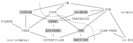
Figure 3. The inclusions between the considered graph classes. We characterize the automorphism groups of the classes in gray.

Outline. In Section 2, we introduce notation and group products. In Section 3, we explain our general technique for determining the automorphism group from the geometric structure of all representations, and relate it to map theory. We describe the automorphism groups of interval and unit interval graphs in Section 4, of circle graphs in Section 5, and of permutation and bipartite permutation graphs in Section 6. Our results are constructive and lead to polynomial-time algorithms computing automorphism groups of these graph classes; see Section 7. We conclude with several open problems.

2. Preliminaries

We use $X$ and $Y$ for graphs, $M$, $T$ and $S$ for trees and $G$ and $H$ for groups. The vertices and edges of $X$ are $V(X)$ and $E(X)$. For $A\subseteq V(X)$, we denote by $X[A]$ the subgraph induced by $A$, and for $x\in V(X)$, the closed neighborhood of $x$ by $N[x]$. The complement of $X$ is denoted by $\overline{X}$, clearly ${\rm Aut}(X)={\rm Aut}(\overline{X})$.

A permutation $\pi$ of $V(X)$ is an automorphism if $uv\in E(X)\iff\pi(u)\pi(v)\in E(X)$. The automorphism group ${\rm Aut}(X)$ consists of all automorphisms of $X$. We use the notation $\mathbb{S}_{n}$, $\mathbb{D}_{n}$ and $\mathbb{Z}_{n}$ for the symmetric, dihedral and cyclic groups. Note that $\mathbb{D}_{1}\cong\mathbb{Z}_{2}$ and $\mathbb{D}_{2}\cong\mathbb{Z}_{2}^{2}$ (which appears in Theorems 1.4 and 1.5 in (d)). An action is called semiregular if all stabilizers are trivial.

Group Products. Group products allow decomposing of large groups into smaller ones. Given two groups $N$ and $H$, and a group homomorphism $\varphi\colon H\to{\rm Aut}(N)$, we can construct a new group $N\rtimes_{\varphi}H$ as the Cartesian product $N\times H$ with the operation defined as $(n_{1},h_{1})\cdot(n_{2},h_{2})=(n_{1}\cdot\varphi(h_{1})(n_{2}),h_{1}\cdot h_{2})$. The group $N\rtimes_{\varphi}H$ is called the external semidirect product of $N$ and $H$ with respect to the homomorphism $\varphi$, and sometimes we omit the homomorphism $\varphi$ and write $N\rtimes H$. Alternatively, $G$ is the internal semidirect product of $N$ and $H$ if $N\unlhd G$, $H\leq G$, $N\cap H$ is trivial and $\left<N\cup H\right>=G$.

Suppose that $H$ acts on $\{1,\dots,n\}$. The wreath product $G\wr H$ is a shorthand for the semidirect product $G^{n}\rtimes_{\psi}H$ where $\psi$ is defined naturally by $\psi(\pi)=(g_{1},\dots,g_{n})\mapsto(g_{\pi(1)},\dots,g_{\pi(n)})$. In the paper, we have $H$ equal $\mathbb{S}_{n}$ or $\mathbb{Z}_{n}$ for which we use the natural actions on $\{1,\dots,n\}$. For more details, see [5, 35]. All semidirect products used in this paper are generalized wreath products of $G_{1},\dots,G_{k}$ with $H$, in which each orbit of the action of $H$ has assigned one group $G_{i}$.

2.1. Automorphism Groups of Disconnected Graphs.

In 1869, Jordan described the automorphism groups of disconnected graphs, in terms of the automorphism groups of their connected components. Since a similar argument is used in several places in this paper, we describe his proof in details. Figure 4 shows the automorphism group for a graph consisting of two isomorphic components.

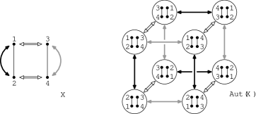
Figure 4. The structure of ${\rm Aut}(X)$, generated by three involutions acting on $X$ on the left: ${\rm Aut}(X)\cong\mathbb{Z}_{2}^{2}\rtimes\mathbb{Z}_{2}=\mathbb{Z}_{2}\wr\mathbb{Z}_{2}$.

Theorem 2.1 (Jordan [26]).

If $X_{1},\dots,X_{n}$ are pairwise non-isomorphic connected graphs and $X$ is the disjoint union of $k_{i}$ copies of $X_{i}$, then

$${\rm Aut}(X)\cong{\rm Aut}(X_{1})\wr\mathbb{S}_{k_{1}}\times\cdots\times{\rm Aut}(X_{n})\wr\mathbb{S}_{k_{n}}.$$

Proof.

Since the action of ${\rm Aut}(X)$ is independent on non-isomorphic components, it is clearly the direct product of factors, each corresponding to the automorphism group of one isomorphism class of components. It remains to show that if $X$ consists of $k$ isomorphic components of a connected graph $Y$, then ${\rm Aut}(X)\cong{\rm Aut}(Y)\wr\mathbb{S}_{k}$.

We isomorphically label the vertices of each component. Then each automorphism $\pi\in{\rm Aut}(X)$ is a composition $\sigma\cdot\tau$ of two automorphisms: $\sigma$ maps each component to itself, and $\tau$ permutes the components as in $\pi$ while preserving the labeling. Therefore, the automorphisms $\sigma$ can be bijectively identified with the elements of ${\rm Aut}(Y)^{k}$ and the automorphisms $\tau$ with the elements of $\mathbb{S}_{k}$.

Let $\pi,\pi^{\prime}\in{\rm Aut}(X)$. Consider the composition $\sigma\cdot\tau\cdot\sigma^{\prime}\cdot\tau^{\prime}$, we want to swap $\tau$ with $\sigma^{\prime}$ and rewrite this as a composition $\sigma\cdot\hat{\sigma}\cdot\hat{\tau}\cdot\tau$. Clearly the components are permuted in $\pi\cdot\pi^{\prime}$ exactly as in $\tau\cdot\tau^{\prime}$, so $\hat{\tau}=\tau$. On the other hand, $\hat{\sigma}$ is not necessarily equal $\sigma^{\prime}$. Let $\sigma^{\prime}$ be identified with the vector $(\sigma_{1}^{\prime},\dots,\sigma_{k}^{\prime})\in{\rm Aut}(Y)^{k}$. Since $\sigma^{\prime}$ is applied after $\tau$, it acts on the components permuted according to $\tau$. Therefore $\hat{\sigma}$ is constructed from $\sigma^{\prime}$ by permuting the coordinates of its vector by $\tau$:

$$\hat{\sigma}=(\sigma^{\prime}_{\tau(1)},\dots,\sigma^{\prime}_{\tau(k)}).$$

This is precisely the definition of the wreath product, so ${\rm Aut}(X)\cong{\rm Aut}(Y)\wr\mathbb{S}_{k}$. ∎

2.2. Automorphism Groups of Trees.

Using the above, we can explain why ${\rm Aut}(\hbox{\rm TREE})$ is closed under (b) and (c):

Proof of Theorem 1.2 (a sketch).

We assume that trees are rooted since the automorphism groups preserve centers. Every inductively defined group can be realized by a tree as follows. For the direct product in (b), we choose two non-isomorphic trees $T_{1}$ and $T_{2}$ with ${\rm Aut}(T_{i})\cong G_{i}$, and attach them to a common root. For the wreath product in (c), we take $n$ copies of a tree $T$ with ${\rm Aut}(T)\cong G$ and attach them to a common root. On the other hand, given a rooted tree, we can delete the root and apply Theorem 2.1 to the created forest of rooted trees. ∎

3. Automorphism Groups Acting on Intersection Representations

In this section, we describe the general technique which allows us to geometrically understand automorphism groups of some intersection-defined graph classes. Suppose that one wants to understand an abstract group $G$. Sometimes, it is possible interpret $G$ using a natural action on some set which is easier to understand. The action is called faithful if no element of $G$ belongs to all stabilizers. The structure of $G$ is captured by a faithful action. We require that this action is “faithful enough”, which means that the stabilizers are simple and can be understood.

Our approach is inspired by map theory. A map ${\mathcal{M}}$ is a 2-cell embedding of a graph; i.e, aside vertices and edges, it prescribes a rotational scheme for the edges incident with each vertex. One can consider the action of ${\rm Aut}(X)$ on the set of all maps of $X$: for $\pi\in{\rm Aut}(X)$, we get another map $\pi({\mathcal{M}})$ in which the edges in the rotational schemes are permuted by $\pi$; see Fig. 5. The stabilizer of a map ${\mathcal{M}}$, called the automorphism group ${\rm Aut}({\mathcal{M}})$, is the subgroup of ${\rm Aut}(X)$ which preserves/reflects the rotational schemes. Unlike ${\rm Aut}(X)$, we know that ${\rm Aut}({\mathcal{M}})$ is always small (since ${\rm Aut}({\mathcal{M}})$ acts semiregularly on flags) and can be efficiently determined. The action of ${\rm Aut}(X)$ describes morphisms between different maps and in general can be very complicated. Using this approach, the automorphism groups of planar graphs can be characterized [1, 27].

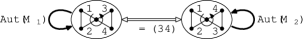
Figure 5. There are two different maps, depicted with the action of ${\rm Aut}(X)$. The stabilizers ${\rm Aut}({\mathcal{M}}_{i})\cong\mathbb{Z}_{2}^{2}$ are normal subgroups. The remaining automorphisms morph one map into the other, for instance $\pi$ transposing $2$ and $3$. We have ${\rm Aut}(X)\cong\mathbb{Z}_{2}^{2}\rtimes\mathbb{Z}_{2}$.

The Induced Action. For a graph $X$, we denote by $\mathfrak{Rep}$ the set of all its (interval, circle, etc.) intersection representations. An automorphism $\pi\in{\rm Aut}(X)$ creates from ${\mathcal{R}}\in\mathfrak{Rep}$ another representation ${\mathcal{R}}^{\prime}$ such that $R^{\prime}_{\pi(u)}=R_{u}$; so $\pi$ swaps the labels of the sets of ${\mathcal{R}}$. We denote ${\mathcal{R}}^{\prime}$ as $\pi({\mathcal{R}})$, and ${\rm Aut}(X)$ acts on $\mathfrak{Rep}$.

The general set $\mathfrak{Rep}$ is too large. Therefore, we define a suitable equivalence relation $\sim$ and we work with $\mathfrak{Rep}/\mathord{\sim}$. It is reasonable to assume that $\sim$ is a congruence with respect to the action of ${\rm Aut}(X)$: for every ${\mathcal{R}}\sim{\mathcal{R}}^{\prime}$ and $\pi\in{\rm Aut}(X)$, we have $\pi({\mathcal{R}})\sim\pi({\mathcal{R}}^{\prime})$. We consider the induced action of ${\rm Aut}(X)$ on $\mathfrak{Rep}/\mathord{\sim}$.

The stabilizer of ${\mathcal{R}}\in\mathfrak{Rep}/\mathord{\sim}$, denoted by ${\rm Aut}({\mathcal{R}})$, describes automorphisms inside this representation. For a nice class of intersection graphs, such as interval, circle or permutation graphs, the stabilizers ${\rm Aut}({\mathcal{R}})$ are very simple. If it is a normal subgroup, then the quotient ${\rm Aut}(X)/{\rm Aut}({\mathcal{R}})$ describes all morphisms which change one representation in the orbit of ${\mathcal{R}}$ into another one. Our strategy is to understand these morphisms geometrically, for which we use the structure of all representations, encoded for the considered classes by PQ-, split and modular trees.

4. Automorphism Groups of Interval Graphs

In this section, we prove Theorem 1.3. We introduce an MPQ-tree which combinatorially describe all interval representations of a given interval graph. We define its automorphism group, which is a quotient of the automorphism group of the interval graph. Using MPQ-trees, we derive a characterization of ${\rm Aut}(\hbox{\rm INT})$ which we prove to be equivalent to the Jordan’s characterization of ${\rm Aut}(\hbox{\rm TREE})$. Finally, we solve Hanlon’s open problem [23] by constructing for a given interval graph a tree with the same automorphism group, and we also show the converse construction.

4.1. PQ- and MPQ-trees

We denote the set of all maximal cliques of $X$ by ${\mathcal{C}}(X)$. In 1965, Fulkerson and Gross proved the following fundamental characterization of interval graphs by orderings of maximal cliques:

Lemma 4.1 (Fulkerson and Gross [15]).

A graph $X$ is an interval graph if and only if there exists a linear ordering $\preceq$ of ${\mathcal{C}}(X)$ such that for every $x\in V(X)$ the maximal cliques containing $x$ appear consecutively in this ordering.

Sketch of proof.

Let ${\mathcal{R}}=\bigl{\{}R_{x}\colon x\in V(X)\bigr{\}}$ be an interval representation of $X$ and let ${\mathcal{C}}(X)=\{C_{1},\dots,C_{k}\}$. By Helly’s Theorem, the intersection $\bigcap_{x\in C_{i}}R_{x}$ is non-empty, and therefore it contains a point $c_{i}$. The ordering of $c_{1},\dots,c_{k}$ from left to right gives the ordering $\preceq$.

For the other implication, given an ordering $C_{1}\preceq\cdots\preceq C_{k}$ of the maximal cliques, we place points $c_{1},\dots,c_{k}$ in this ordering on the real line. To each vertex $x$, we assign the minimal interval $R_{x}$ such that $c_{i}\in R_{x}$ for all $x\in C_{i}$. We obtain a valid interval representation $\bigl{\{}R_{x}\colon x\in V(X)\bigr{\}}$ of $X$. ∎

An ordering $\preceq$ of ${\mathcal{C}}(X)$ from Lemma 4.1 is called a consecutive ordering. Consecutive orderings of ${\mathcal{C}}(X)$ correspond to different interval representations of $X$.

PQ-trees. Booth and Lueker [4] invented a data structure called a PQ-tree which encodes all consecutive orderings of an interval graph. They build this structure to construct a linear-time algorithm for recognizing interval graphs which was a long standing open problem. PQ-trees give a lot of insight into the structure of all interval representations, and have applications to many problems. We use them to capture the automorphism groups of interval graphs.

A rooted tree $T$ is a PQ-tree representing an interval graph $X$ if the following holds. It has two types of inner nodes: P-nodes and Q-nodes. For every inner node, its children are ordered from left to right. Each P-node has at least two children and each Q-node at least three. The leaves of $T$ correspond one-to-one to ${\mathcal{C}}(X)$. The frontier of $T$ is the ordering $\preceq$ of the leaves from left to right.

Two PQ-trees are equivalent if one can be obtained from the other by a sequence of two equivalence transformations: (i) an arbitrary permutation of the order of the children of a P-node, and (ii) the reversal of the order of the children of a Q-node. The consecutive orderings of ${\mathcal{C}}(X)$ are exactly the frontiers of the PQ-trees equivalent with $T$. Booth and Lueker [4] proved the existence and uniqueness of PQ-trees (up to equivalence transformations). Figure 6 shows an example.

For a PQ-tree $T$, we consider all sequences of equivalent transformations. Two such sequences are congruent if they transform $T$ the same. Each sequence consists of several transformations of inner nodes, and it is easy to see that these transformation are independent. If a sequence transforms one inner node several times, it can be replaced by a single transformation of this node. Let $\Sigma(T)$ be the quotient of all sequences of equivalent transformations of $T$ by this congruence. We can represent each class by a sequence which transforms each node at most once.

Observe that $\Sigma(T)$ forms a group with the concatenation as the group operation. This group is isomorphic to a direct product of symmetric groups. The order of $\Sigma(T)$ is equal to the number of equivalent PQ-trees of $T$. Let $T^{\prime}=\sigma(T)$ for some $\sigma\in\Sigma(T)$. Then $\Sigma(T^{\prime})\cong\Sigma(T)$ since $\sigma^{\prime}\in\Sigma(T^{\prime})$ corresponds to $\sigma\sigma^{\prime}\sigma^{-1}\in\Sigma(T)$.

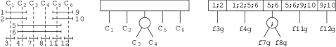
Figure 6. An ordering of the maximal cliques, and the corresponding PQ-tree and MPQ-tree. The P-nodes are denoted by circles, the Q-nodes by rectangles. There are four different consecutive orderings.

MPQ-trees. A modified PQ-tree is created from a PQ-tree by adding information about the vertices. They were described by Korte and Möhring [29] to simplify linear-time recognition of interval graphs. It is not widely known but the equivalent idea was used earlier by Colbourn and Booth [8].

Let $T$ be a PQ-tree representing an interval graph $X$. We construct the MPQ-tree $M$ by assigning subsets of $V(X)$, called sections, to the nodes of $T$; see Fig. 6. The leaves and the P-nodes have each assigned exactly one section while the Q-nodes have one section per child. We assign these sections as follows:

• For a leaf $L$, the section ${\rm sec}(L)$ contains those vertices that are only in the maximal clique represented by $L$, and no other maximal clique.

• For a P-node $P$, the section ${\rm sec}(P)$ contains those vertices that are in all maximal cliques of the subtree of $P$, and no other maximal clique.

• For a Q-node $Q$ and its children $T_{1},\dots,T_{n}$, the section ${\rm sec}_{i}(Q)$ contains those vertices that are in the maximal cliques represented by the leaves of the subtree of $T_{i}$ and also some other $T_{j}$, but not in any other maximal clique outside the subtree of $Q$. We put ${\rm sec}(Q)={\rm sec}_{1}(Q)\cup\cdots\cup{\rm sec}_{n}(Q)$.

Korte and Möhring [29] proved existence of MPQ-trees and many other properties, for instance each vertex appears in sections of exactly one node and in the case of a Q-node in consecutive sections. Two vertices are in the same sections if and only if they belong to precisely the same maximal cliques. Figure 6 shows an example.

We consider the equivalence relation $\thicksim_{TW}$ on $V(X)$ is defined as follows: $x\thicksim_{TW}y$ if and only if $N[x]=N[y]$. If $x\thicksim_{TW}y$, then we say that they are twin vertices. The equivalence classes of $\thicksim_{TW}$ are called twin classes. Twin vertices can usually be ignored, but they influence the automorphism group. Two vertices belong to the same sections if and only if they are twin vertices.

4.2. Automorphisms of MPQ-trees

For a graph $X$, the automorphism group ${\rm Aut}(X)$ induces an action on ${\mathcal{C}}(X)$ since every automorphism permutes the maximal cliques. If $X$ is an interval graph, then a consecutive ordering $\preceq$ of ${\mathcal{C}}(X)$ is permuted into another consecutive ordering $\pi(\preceq)$, so ${\rm Aut}(X)$ acts on consecutive orderings.

Suppose that an MPQ-tree $M$ representing $X$ has the frontier $\preceq$. For every automorphism $\pi\in{\rm Aut}(X)$, there exists the unique MPQ-tree $M^{\prime}$ with the frontier $\pi(\preceq)$ which is equivalent to $M$. We define a mapping

$$\Phi:{\rm Aut}(X)\to\Sigma(M)$$

such that $\Phi(\pi)$ is the sequence of equivalent transformations which transforms $M$ to $M^{\prime}$. It is easy to observe that $\Phi$ is a group homomorphism.

By Homomorphism Theorem, we know that ${\rm Im}(\Phi)\cong{\rm Aut}(X)/{\rm Ker}(\Phi)$. The kernel ${\rm Ker}(\Phi)$ consists of all automorphisms which fix the maximal cliques, so they permute the vertices inside each twin class. It follows that ${\rm Ker}(\Phi)$ is isomorphic to a direct product of symmetric groups. So ${\rm Im}(\Phi)$ almost describes ${\rm Aut}(X)$.

Two MPQ-trees $M$ and $M^{\prime}$ are isomorphic if the underlying PQ-trees are equal and there exists a permutation $\pi$ of $V(X)$ which maps each section of $M$ to the corresponding section of $M^{\prime}$. In other words, $M$ and $M^{\prime}$ are the same when ignoring the labels of the vertices in the sections. A sequence $\sigma\in\Sigma(M)$ is called an automorphism of $M$ if $\sigma(M)\cong M$; see Fig. 7. The automorphisms of $M$ are closed under composition, so they form the automorphism group ${\rm Aut}(M)\leq\Sigma(M)$.

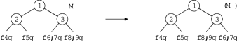
Figure 7. The sequence $\sigma$, which transposes the children of the P-node with the section $\{3\}$, is an automorphism since $\sigma(M)\cong M$. On the other, the transposition of the children the root P-node is not an automorphism.

Lemma 4.2.

For an MPQ-tree $M$, we have ${\rm Aut}(M)={\rm Im}(\Phi)$.

Proof.

Suppose that $\pi\in{\rm Aut}(X)$. The sequence $\sigma=\Phi(\pi)$ transforms $M$ into $\sigma(M)$. It follows that $\sigma(M)\cong M$ since $\sigma(M)$ can be obtained from $M$ by permuting the vertices in the sections by $\pi$. So $\sigma\in{\rm Aut}(M)$ and ${\rm Im}(\Phi)\leq{\rm Aut}(M)$.

On the other hand, suppose $\sigma\in{\rm Aut}(M)$. We know that $\sigma(M)\cong M$ and let $\pi$ be a permutation of $V(X)$ from the definition of the isomorphism. Two vertices of $V(X)$ are adjacent if and only if they belong to the sections of $M$ on a common path from the root. This property is preserved in $\sigma(M)$, so $\pi\in{\rm Aut}(X)$. Each maximal clique is the union of all sections on the path from the root to the leaf representing this clique. Therefore the maximal cliques are permuted by $\sigma$ the same as by $\pi$. Thus $\Phi(\pi)=\sigma$ and ${\rm Aut}(M)\leq{\rm Im}(\Phi)$. ∎

Lemma 4.3.

For an MPQ-tree $M$ representing an interval graph $X$, we have ${\rm Aut}(X)\cong{\rm Ker}(\Phi)\rtimes{\rm Aut}(M)$.

Proof.

Let $\sigma\in{\rm Aut}(M)$. In the proof of Lemma 4.2, we show that every permutation $\pi$ from the definition of $\sigma(M)\cong M$ is an automorphism of $X$ mapped by $\Phi$ to $\sigma$. Now, we want to choose these permutations consistently for all elements of ${\rm Aut}(M)$ as follows. Suppose that ${\rm id}=\sigma_{1},\sigma_{2},\dots,\sigma_{n}$ be the elements of ${\rm Aut}(M)$. We want to find ${\rm id}=\pi_{1},\pi_{2},\dots,\pi_{n}$ such that $\Phi(\pi_{i})=\sigma_{i}$ and if $\sigma_{i}\sigma_{j}=\sigma_{k}$, then $\pi_{i}\pi_{j}=\pi_{k}$. In other words, $H=\{\pi_{1},\dots,\pi_{n}\}$ is a subgroup of ${\rm Aut}(X)$ and $\Phi\restriction_{H}$ is an isomorphism between $H$ and ${\rm Aut}(M)={\rm Im}(\Phi)$.

Suppose that $\pi,\pi^{\prime}\in{\rm Aut}(X)$ such that $\Phi(\pi)=\Phi(\pi^{\prime})$. Then $\pi$ and $\pi^{\prime}$ permute the maximal cliques the same and they can only act differently on twin vertices, i.e., $\pi\pi^{\prime-1}\in{\rm Ker}(\Phi)$. Suppose that $C$ is a twin class, then $\pi(C)=\pi^{\prime}(C)$ but they can map the vertices of $C$ differently. To define $\pi_{1},\dots,\pi_{n}$, we need to define them on the vertices of the twin classes consistently. To do so, we arbitrarily order the vertices in each twin class. For each $\pi_{i}$, we know how it permutes the twin classes, suppose a twin class $C$ is mapped to a twin class $\pi_{i}(C)$. Then we define $\pi_{i}$ on the vertices of $C$ in such a way that the orderings are preserved.

The above construction of $H$ is correct. Since $H$ is the complementary subgroup of ${\rm Ker}(\Phi)$, we get ${\rm Aut}(X)$ as the internal semidirect product ${\rm Ker}(\Phi)\rtimes H\cong{\rm Ker}(\Phi)\rtimes{\rm Aut}(M)$. Our approach is similar to the proof of Theorem 2.1, and the external semidirect product can be constructed in the same way. ∎

4.3. The Inductive Characterization

Let $X$ be an interval graph, represented by an MPQ-tree $M$. By Lemma 4.3, ${\rm Aut}(X)$ can be described from ${\rm Aut}(M)$ and ${\rm Ker}(\Phi)$. We build ${\rm Aut}(X)$ inductively using $M$, similarly as in Theorem 1.2:

Proof of Theorem 1.3(i).

We show that ${\rm Aut}(\hbox{\rm INT})$ is closed under (b), (c) and (d); see Fig. 8. For (b), we attach interval graphs $X_{1}$ and $X_{2}$ such that ${\rm Aut}(X_{i})=G_{i}$ to an asymmetric interval graph. For (c), let $G\in{\rm Aut}(\hbox{\rm INT})$ and let $Y$ be a connected interval graph with ${\rm Aut}(Y)\cong G$. We construct $X$ as the disjoint union of $n$ copies of $Y$. For (d), we construct $X$ by attaching $X_{1}$ and $X_{2}$ to a path, where ${\rm Aut}(X_{i})=G_{i}$.

Figure 8. The constructions in the proof of Theorem 1.3(i).

For the converse, let $M$ be an MPQ-tree representing an interval graph $X$. Let $M_{1},\dots,M_{k}$ be the subtrees of the root of $M$ and let $X_{i}$ be the interval graphs induced by the vertices of the sections of $M_{i}$. We want to build ${\rm Aut}(X)$ from ${\rm Aut}(X_{1}),\dots,{\rm Aut}(X_{k})$ using (b) to (d).

Case 1: The root is a P-node $P$. Each sequence $\sigma\in{\rm Aut}(M)$ corresponds to interior sequences in ${\rm Aut}(M_{i})$ and some reordering $\sigma^{\prime}$ of $M_{1},\dots,M_{k}$. If $\sigma^{\prime}(M_{i})=M_{j}$, then necessarily $X_{i}\cong X_{j}$. On each isomorphism class of $X_{1},\dots,X_{k}$, the permutations $\sigma^{\prime}$ behave to ${\rm Aut}(X_{i})$ like the permutations $\tau$ to ${\rm Aut}(Y)$ in the proof of Theorem 2.1. Therefore the point-wise stabilizer of ${\rm sec}(P)$ in ${\rm Aut}(X)$ is constructed from ${\rm Aut}(X_{1}),\dots,{\rm Aut}(X_{k})$ as in Theorem 2.1. Since every automorphim preserves ${\rm sec}(P)$, then ${\rm Aut}(X)$ is obtained by the direct product of the above group with the symmetric group of order $|{\rm sec}(P)|$. Thus the operations (b) and (c) are sufficient.

Case 2: The root is a Q-node $Q$. We call $Q$ symmetric if it is transformed by some sequence of ${\rm Aut}(M)$, and asymmetric otherwise. Let $M_{1},\dots,M_{k}$ be its children from left to right. If $Q$ is asymmetric, then ${\rm Aut}(M)$ is the direct product ${\rm Aut}(X_{1}),\dots,{\rm Aut}(X_{k})$ together with the symmetric groups for all twin classes of ${\rm sec}(Q)$, so it can be build using (b). If $Q$ is symmetric, let $G_{1}$ is the direct product of the left part of the children and twin classes, and $G_{2}$ of the middle part. We get

$${\rm Aut}(X)\cong(G_{1}^{2}\times G_{2})\rtimes\mathbb{Z}_{2}\cong G_{1}^{2}\rtimes\mathbb{Z}_{2}\times G_{2}\cong G_{1}\wr\mathbb{Z}_{2}\times G_{2},$$

where the wreath product with $\mathbb{Z}_{2}$ adds the automorphisms reversing $Q$, corresponding to reversing of vertically symmetric parts of a representation. Therefore ${\rm Aut}(X)$ can be generated using (b) and (c). ∎

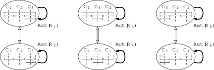
Figure 9. An interval graph with six non-equivalent representation. The action of ${\rm Aut}(X)$ has three isomorphic orbits.

4.4. The Action on Interval Representations.

For an interval graph $X$, the set $\mathfrak{Rep}$ consists of all assignments of closed intervals which define $X$. It is natural to consider two interval representations equivalent if one can be transformed into the other by continuous shifting of the endpoints of the intervals while preserving the correctness of the representation. Then the representations of $\mathfrak{Rep}/\mathord{\sim}$ correspond to consecutive orderings of the maximal cliques; see Fig. 9 and 10.

We interpret our results in terms of the action of ${\rm Aut}(X)$ on $\mathfrak{Rep}$. In Lemma 4.3, we proved that ${\rm Aut}(X)\cong{\rm Ker}(\Phi)\rtimes{\rm Aut}(M)$ where $M$ is an MPQ-tree. If an automorphism belongs to ${\rm Aut}({\mathcal{R}})$, then it fixes the ordering of the maximal cliques and it can only permute twin vertices. Therefore ${\rm Aut}({\mathcal{R}})={\rm Ker}(\Phi)$ since each twin class consists of equal intervals, so they can be arbitrarily permuted without changing the representation. Every stabilizer ${\rm Aut}({\mathcal{R}})$ is the same and every orbit of the action of ${\rm Aut}(X)$ is isomorphic, as in Fig. 9.

Different orderings of the maximal cliques correspond to different reorderings of $M$. The defined ${\rm Aut}(M)\cong{\rm Aut}(X)/{\rm Aut}({\mathcal{R}})$ describes morphisms of representations belonging to one orbit of the action of ${\rm Aut}(X)$, which are the same representations up to the labeling of the intervals; see Fig. 9 and Fig. 10.

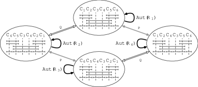
Figure 10. The action of ${\rm Aut}(X)$ is transitive. An MPQ-tree $M$ of $X$ is depicted in Fig. 6. There are three twin classes of size two, so ${\rm Aut}({\mathcal{R}})\cong\mathbb{Z}_{2}^{3}$. The group ${\rm Aut}(M)$ is generated by $\pi_{Q}$ corresponding to flipping the Q-node, and $\pi_{P}$ permuting the P-node. We have ${\rm Aut}(M)\cong\mathbb{Z}_{2}^{2}$ and ${\rm Aut}(X)\cong\mathbb{Z}_{2}^{3}\rtimes\mathbb{Z}_{2}^{2}$.

4.5. Direct Constructions.

In this section, we explain Theorem 1.3(i) by direct constructions. The first construction answers the open problem of Hanlon [23].

Lemma 4.4.

For $X\in\hbox{\rm INT}$, there exists $T\in\hbox{\rm TREE}$ such that ${\rm Aut}(X)\cong{\rm Aut}(T)$.

Proof.

Consider an MPQ-tree $M$ representing $X$. We know that ${\rm Aut}(X)\cong{\rm Ker}(\Phi)\rtimes{\rm Aut}(M)$ and we inductively encode the structure of $M$ into $T$.

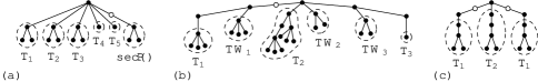
Figure 11. For an interval graph $X$, a construction of a tree $T$ with ${\rm Aut}(T)\cong{\rm Aut}(X)$: (a) The root is a P-node. (b) The root is an asymmetric Q-node. (c) The root is a symmetric Q-node.

Case 1: The root is a P-node $P$. Its subtrees can be encoded by trees and we just attach them to a common root. If ${\rm sec}(P)$ is non-empty, we attach a star with $|{\rm sec}(P)|$ leaves to the root (and we subdivide it to make it non-isomorphic to every other subtree attached to the root); see Fig 11a. We get ${\rm Aut}(T)\cong{\rm Aut}(X)$.

Case 2: The root is a Q-node $Q$. If $Q$ is asymmetric, we attach the trees corresponding to the subtrees of $Q$ and stars corresponding to the vertices of twin classes in the sections of $Q$ to a path, and possibly modify by subdivisions to make it asymmetric; see Fig. 11b. And if $Q$ is symmetric, then ${\rm Aut}(X)\cong(G_{1}^{2}\times G_{3})\rtimes\mathbb{Z}_{2}$ and we just attach trees $T_{1}$ and $T_{2}$ such that ${\rm Aut}(T_{i})\cong G_{i}$ to a path as in Fig. 11c. In both cases, ${\rm Aut}(T)\cong{\rm Aut}(X)$. ∎

Lemma 4.5.

For $T\in\hbox{\rm TREE}$, there exists $X\in\hbox{\rm INT}$ such that ${\rm Aut}(T)\cong{\rm Aut}(X)$.

Proof.

For a rooted tree $T$, we construct an interval graph $X$ such that ${\rm Aut}(T)\cong{\rm Aut}(X)$ as follows. The intervals are nested according to $T$ as shown in Fig. 12. Each interval is contained exactly in the intervals of its ancestors. If $T$ contains a vertex with only one child, then ${\rm Aut}(T)<{\rm Aut}(X)$. This can be fixed by adding suitable asymmetric interval graphs $Y$, as in Fig. 12. ∎

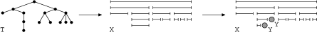
Figure 12. We place the intervals following the structure of the tree. We get ${\rm Aut}(X)\cong\mathbb{S}_{3}\times\mathbb{S}_{2}\times\mathbb{S}_{3}$, but ${\rm Aut}(T)\cong\mathbb{S}_{2}\times\mathbb{S}_{3}$. We fix this by attaching asymmetric interval graphs $Y$.

4.6. Automorphism Groups of Unit Interval Graphs

We apply the characterization of ${\rm Aut}(\hbox{\rm INT})$ derived in Theorem 1.3(i) to show that the automorphism groups of connected unit interval graphs are the same of caterpillars (which form the intersection of INT and TREE). The reader can make direct constructions, similarly as in Lemmas 4.4 and 4.5. First, we describe ${\rm Aut}(\hbox{\rm CATERPILLAR})$:

Lemma 4.6.

The class ${\rm Aut}(\hbox{\rm CATERPILLAR})$ consists of all groups $G_{1}$ and $G_{1}\wr\mathbb{Z}_{2}\times G_{2}$ where $G_{1}$ is a direct product of symmetric groups and $G_{2}$ is a symmetric group.

Proof.

We can easily construct caterpillars with these automorphism groups. On the other hand, the root of an MPQ-tree $M$ representing $T$ is a Q-node $Q$ (or a P-node with at most two children, which is trivial). All twin classes are trivial, since $T$ is a tree. Each child of the root is either a P-node, or a leaf. All children of a P-node are leaves. We can determine ${\rm Aut}(X)$ as in the proof of Theorem 1.3(i). ∎

Proof of Theorem 1.3(ii).

According to Corneil [9], an MPQ-tree $M$ representing a connected unit interval graph contains only one Q-node with all children as leaves. It is possible that the sections of this Q-node are nontrivial. This equality of automorphism groups follows by Lemma 4.6 and the proof of Theorem 1.3(i). ∎

5. Automorphism Groups of Circle Graphs

In this section, we prove Theorem 1.4. We introduce the split decomposition which was invented for recognizing circle graphs. We encode the split decomposition of $X$ by a split tree $S$ which captures all circle representations of $X$. We define automorphisms of $S$ and show that ${\rm Aut}(S)\cong{\rm Aut}(X)$.

5.1. Split Decomposition

A split is a partition $(A,B,A^{\prime},B^{\prime})$ of $V(X)$ such that:

• For every $a\in A$ and $b\in B$, we have $ab\in E(X)$.

• There are no edges between $A^{\prime}$ and $B\cup B^{\prime}$, and between $B^{\prime}$ and $A\cup A^{\prime}$.

• Both sides have at least two vertices: $|A\cup A^{\prime}|\geq 2$ and $|B\cup B^{\prime}|\geq 2$.

The split decomposition of $X$ is constructed by taking a split of $X$ and replacing $X$ by the graphs $X_{A}$ and $X_{B}$ defined as follows. The graph $X_{A}$ is created from $X[A\cup A^{\prime}]$ together with a new marker vertex $m_{A}$ adjacent exactly to the vertices in $A$. The graph $X_{B}$ is defined analogously for $B$, $B^{\prime}$ and $m_{B}$; see Fig. 13a. The decomposition is then applied recursively on $X_{A}$ and $X_{B}$. Graphs containing no splits are called prime graphs. We stop the split decomposition also on degenerate graphs which are complete graphs $K_{n}$ and stars $K_{1,n}$. A split decomposition is called minimal if it is constructed by the least number of splits. Cunningham [10] proved that the minimal split decomposition of a connected graph is unique.

The key connection between the split decomposition and circle graphs is the following: a graph $X$ is a circle graph if and only if both $X_{A}$ and $X_{B}$ are. In a other words, a connected graph $X$ is a circle graph if and only if all prime graphs obtained by the minimal split decomposition are circle graphs.

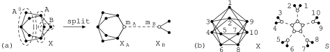
Figure 13. (a) An example of a split of the graph $X$. The marker vertices are depicted in white. The tree edge is depicted by a dashed line. (b) The split tree $S$ of the graph $X$. We have that ${\rm Aut}(S)\cong\mathbb{Z}_{2}^{5}\rtimes\mathbb{D}_{5}$.

Split tree. The split tree $S$ representing a graph $X$ encodes the minimal split decomposition. A split tree is a graph with two types of vertices (normal and marker vertices) and two types of edges (normal and tree edges). We initially put $S=X$ and modify it according to the minimal split decomposition. If the minimal decomposition contains a split $(A,B,A^{\prime},B^{\prime})$ in $Y$, then we replace $Y$ in $S$ by the graphs $Y_{A}$ and $Y_{B}$, and connect the marker vertices $m_{A}$ and $m_{B}$ by a tree edge (see Fig. 13a). We repeat this recursively on $Y_{A}$ and $Y_{B}$; see Fig. 13b. Each prime and degenerate graph is a node of the split tree. Since the minimal split decomposition is unique, we also have that the split tree is unique.

Next, we prove that the split tree $S$ captures the adjacencies in $X$.

Lemma 5.1.

We have $xy\in E(X)$ if and only if there exists an alternating path $xm_{1}m_{2}\dots m_{k}y$ in $S$ such that each $m_{i}$ is a marker vertex and precisely the edges $m_{2i-1}m_{2i}$ are tree edges.

Proof.

Suppose that $xy\in E(X)$. We prove existence of an alternating path between $x$ and $y$ by induction according to the length of this path. If $xy\in E(S)$, then it clearly exists. Otherwise the split tree $S$ was constructed by applying a split decomposition. Let $Y$ be the graph in this decomposition such that $xy\in E(Y)$ and there is a split $(A,B,A^{\prime},B^{\prime})$ in $Y$ in this decomposition such that $x\in A$ and $y\in B$. We have $x\in V(Y_{A})$, $xm_{A}\in E(Y_{A})$, $y\in V(Y_{B})$, and $ym_{B}\in E(Y_{B})$. By induction hypothesis, there exist alternating paths between $x$ and $m_{A}$ and between $m_{B}$ and $y$ in $S$. There is a tree edge $m_{A}m_{B}$, so by joining we get an alternating path between $x$ and $y$. On the other hand, if there exists an alternating path $xm_{1}\dots m_{k}y$ in $S$, by joining all splits, we get $xy\in E(X)$. ∎

5.2. Automorphisms of Split-trees

In [18], split trees are defined in terms of graph-labeled trees. Our definition is more suitable for automorphisms. An automorphism of a split tree $S$ is an automorphism of $S$ which preserves the types of vertices and edges, i.e, it maps marker vertices to marker vertices, and tree edges to tree edges. We denote the automorphism group of $S$ by ${\rm Aut}(S)$.

Lemma 5.2.

If $S$ is a split tree representing a graph $X$, then ${\rm Aut}(S)\cong{\rm Aut}(X)$.

Proof.

First, we show that each $\sigma\in{\rm Aut}(S)$ induces a unique automorphism $\pi$ of $X$. Since $V(X)\subseteq V(S)$, we define $\pi=\sigma\restriction_{V(X)}$. By Lemma 5.1, $xy\in E(X)$ if and only if there exists an alternating path between them in $S$. Automorphisms preserve alternating paths, so $xy\in E(X)\iff\pi(x)\pi(y)\in E(X)$.

On the other hand, we show that $\pi\in{\rm Aut}(X)$ induces a unique automorphism $\sigma\in{\rm Aut}(S)$. We define $\sigma\restriction_{V(X)}=\pi$ and extend it recursively on the marker vertices. Let $(A,B,A^{\prime},B^{\prime})$ be a split of the minimal split decomposition in $X$. This split is mapped by $\pi$ to another split $(C,D,C^{\prime},D^{\prime})$ in the minimal split decomposition, i.e., $\pi(A)=C$, $\pi(A^{\prime})=C^{\prime}$, $\pi(B)=D$, and $\pi(B^{\prime})=D^{\prime}$. By applying the split decomposition to the first split, we get the graphs $X_{A}$ and $X_{B}$ with the marker vertices $m_{A}\in V(X_{A})$ and $m_{B}\in V(X_{B})$. Similarly, for the second split we get $X_{C}$ and $X_{D}$ with $m_{C}\in V(X_{C})$ and $m_{D}\in V(X_{D})$. Since $\pi$ is an automorphism, we have that $X_{A}\cong X_{C}$ and $X_{B}\cong X_{D}$. It follows that the unique split trees of $X_{A}$ and $X_{C}$ are isomorphic, and similarly for $X_{B}$ and $X_{D}$. Therefore, we define $\sigma(m_{A})=m_{C}$ and $\sigma(m_{B})=m_{D}$, and we finish the rest recursively. Since $\sigma$ is an automorphism at each step of the construction of $S$, it follows that $\sigma\in{\rm Aut}(S)$. ∎

Similarly as for trees, there exists a center of $S$ which is either a tree edge, or a prime or degenerate node. If the center is a tree edge, we can modify the split tree by adding two adjacent marker vertices in the middle of the tree edge. This clearly preserves the automorphism group ${\rm Aut}(S)$, so from now on we assume that $S$ has a center $C$ which which is a prime or degenerate node. We can assume that $S$ is rooted by $C$, and for a node $N$, we denote by $S[N]$ the subtree induced by $N$ and its descendants. For $N\neq C$, we call $m$ its root marker vertex if it is the marker vertex of $N$ attached to the parent of $N$.

Recursive Construction. We can describe ${\rm Aut}(S)$ recursively from the leaves to the root $C$. Let $N$ be an arbitrary node of $S$ and consider all its descendants. Let ${\rm Stab}_{S[N]}(x)$ be the subgroup of ${\rm Aut}(S[N])$ which fixes $x\in V(S[N])$. We further color the non-root marker vertices in $N$ by colors coding isomorphism classes of the subtrees attached to them.

Lemma 5.3.

Let $N\neq C$ be a node with the root marker vertex $m$. Let $N_{1},\dots,N_{k}$ be the children of $N$ with the root marker vertices $m_{1},\dots,m_{k}$. Then

$${\rm Stab}_{S[N]}(m)\cong\bigl{(}{\rm Stab}_{S[N_{1}]}(m_{1})\times\cdots\times{\rm Stab}_{S[N_{k}]}(m_{k})\bigr{)}\rtimes{\rm Stab}_{N}(m),$$

where ${\rm Stab}_{N}(m)$ is color preserving.

Proof.

We proceed similarly as in the proof of Theorem 2.1. We isomorphically label the vertices of the isomorphic subtrees $S[N_{i}]$. Each automorphism $\pi\in{\rm Stab}_{S[N]}(m)$ is a composition of two automorphisms $\sigma\cdot\tau$ where $\sigma$ maps each subtree $S[N_{i}]$ to itself, and $\tau$ permutes the subtrees as in $\pi$ while preserving the labeling. Therefore, the automorphisms $\sigma$ can be identified with the elements of the direct product ${\rm Stab}_{S[N_{1}]}(m_{1})\times\cdots\times{\rm Stab}_{S[N_{k}]}(m_{k})$ and the automorphisms $\tau$ with the elements of ${\rm Stab}_{N}(m)$. The rest is exactly as in the proof of Theorem 2.1. ∎

The entire automorphism group ${\rm Aut}(S)$ is obtained by joining these subgroups at the central node $C$. No vertex in $C$ has to be fixed by ${\rm Aut}(S)$.

Lemma 5.4.

Let $C$ be the central node with the children $N_{1},\dots,N_{k}$ with the root marker vertices $m_{1},\dots,m_{k}$. Then

$${\rm Aut}(S)\cong\bigl{(}{\rm Stab}_{S[N_{1}]}(m_{1})\times\cdots\times{\rm Stab}_{S[N_{k}]}(m_{k})\bigr{)}\rtimes{\rm Aut}(C),$$

where ${\rm Aut}(C)$ is color preserving.

Proof.

Similar as the proof of Lemma 5.3. ∎

5.3. The Action On Prime Circle Representations

For a circle graph $X$ with $|V(X)|=\ell$, a representation ${\mathcal{R}}$ is completely determined by a circular word $r_{1}r_{2}\cdots r_{2\ell}$ such that each $r_{i}\in V(X)$ and each vertex appears exactly twice in the word. This word describes the order of the endpoints of the chords in ${\mathcal{R}}$ when the circle is traversed from some point counterclockwise. Two chords intersect if and only if their occurrences alternate in the circular word. Representations are equivalent if they have the same circular words up to rotations and reflections.

The automorphism group ${\rm Aut}(X)$ acts on the circle representations in the following way. Let $\pi\in{\rm Aut}(X)$, then $\pi({\mathcal{R}})$ is the circle representation represented by the word $\pi(r_{1})\pi(r_{2})\cdots\pi(r_{2\ell})$, i.e., the chords are permuted according to $\pi$.

Lemma 5.5.

Let $X$ be a prime circle graph. Then ${\rm Aut}(X)$ is isomorphic to a subgroup of a dihedral group.

Proof.

According to [16], each prime circle graph has a unique representation ${\mathcal{R}}$, up to rotations and reflections of the circular order of endpoints of the chords. Therefore, for every automorphism $\pi\in{\rm Aut}(X)$, we have $\pi({\mathcal{R}})={\mathcal{R}}$, so $\pi$ only rotates/reflects this circular ordering. An automorphism $\pi\in{\rm Aut}(X)$ is called a rotation if there exists $k$ such that $\pi(r_{i})=r_{i+k}$, where the indexes are used cyclically. The automorphisms, which are not rotations, are called reflections, since they reverse the circular ordering. For each reflection $\pi$, there exists $k$ such that $\pi(r_{i})=r_{k-i}$. Notice that composition of two reflections is a rotation. Each reflection either fixes two endpoints in the circular ordering, or none of them.

If no non-identity rotation exists, then ${\rm Aut}(X)$ is either $\mathbb{Z}_{1}$, or $\mathbb{Z}_{2}$. If at least one non-identity rotation exists, let $\rho\in{\rm Aut}(X)$ be the non-identity rotation with the smallest value $k$, called the basic rotation. Observe that $\langle\rho\rangle$ contains all rotations, and if its order is at least three, then the rotations act semiregularly on $X$. If there exists no reflection, then ${\rm Aut}(X)\cong\mathbb{Z}_{n}$. Otherwise, $\langle\rho\rangle$ is a subgroup of ${\rm Aut}(X)$ of index two. Let $\varphi$ be any reflection, then $\rho\varphi\rho=\varphi$ and ${\rm Aut}(X)\cong\mathbb{D}_{n}$. ∎

Lemma 5.6.

Let $X$ be a prime circle graph and let $m\in V(X)$. Then ${\rm Stab}_{X}(m)$ is isomorphic to a subgroup of $\mathbb{Z}_{2}^{2}$.

Proof.

Let $mA\hat{m}B$ be a circular ordering representing $X$, where $m$ and $\hat{m}$ are the endpoints of the chord representing $m$, and $A$ and $B$ are sequences of the endpoints of the remaining chords. We distinguish $m$ and $\hat{m}$ to make the action of ${\rm Stab}_{X}(m)$ understandable. Every $\pi\in{\rm Stab}_{X}(m)$ either fixes both $m$ and $\hat{m}$, or swaps them.

Let $A^{\prime}$ be the reflection of $A$ and $B^{\prime}$ be the reflection of $B$. If both $m$ and $\hat{m}$ are fixed, then by the uniqueness this representation can only be reflected along the chord $m$. If such an automorphism exists in ${\rm Stab}_{X}(m)$, we denote it by $\varphi_{m}$ and we have $\varphi_{m}(mA\hat{m}B)=mB^{\prime}\hat{m}A^{\prime}$. If $m$ and $\hat{m}$ are swapped, then by the uniqueness this representation can be either reflected along the line orthogonal to the chord $m$, or by the $180^{\circ}$ rotation. If these automorphisms exist in ${\rm Stab}_{X}(m)$, we denote them by $\varphi_{\perp}$ and $\rho$, respectively. We have $\varphi_{\perp}(mA\hat{m}B)=\hat{m}A^{\prime}mB^{\prime}$ and $\rho(mA\hat{m}B)=\hat{m}BmA$. Figure 14 shows an example.

Figure 14. A prime circle graph $X$ with ${\rm Stab}_{X}(m)\cong\mathbb{Z}_{2}^{2}$.

All three automorphisms $\varphi_{m}$, $\varphi_{\perp}$ and $\rho$ are involutions, and $\rho=\varphi_{\perp}\cdot\varphi_{m}$. Since ${\rm Stab}_{X}(m)$ is generated by those which exist, it is a subgroup of $\mathbb{Z}_{2}^{2}$. ∎

5.4. The Inductive Characterization

By Lemma 5.2, it is sufficient to determine the automorphism groups of split trees. We proceed from the leaves to the root, similarly as in Theorem 1.2.

Lemma 5.7.

The class $\Sigma$ defined in Theorem 1.4 consists of the following groups:

(5.1) $$\Sigma=\bigl{\{}G:X\in\hbox{\rm connected}\ \hbox{\rm CIRCLE},x\in V(X),G\cong{\rm Stab}_{X}(x)\bigr{\}}.$$

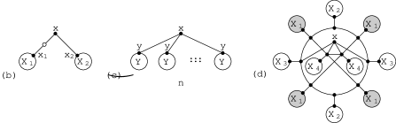
Figure 15. The construction of the group in (d). The eight-cycle in $X$ can be reflected horizontally, vertically and rotated by $180^{\circ}$.

Proof.

First, we show that (5.1) is closed under (b) to (d); see Fig. 15. For (b), let $X_{1}$ and $X_{2}$ be circle graphs such that ${\rm Stab}_{X_{i}}(x_{i})\cong G_{i}$. We construct $X$ as in Fig. 15b, and we get ${\rm Stab}_{X}(x)\cong G_{1}\times G_{2}$. For (c), let $Y$ be a circle graph with ${\rm Stab}_{Y}(y)\cong G$. As $X$, we take $n$ copies of $Y$ and add a new vertex $x$ adjacent to all copies of $y$. Clearly, we get ${\rm Stab}_{X}(x)\cong G\wr\mathbb{S}_{n}$. For (d), let $G_{1},G_{2},G_{3},G_{4}\in\Sigma$, and let $X_{i}$ be a circle graph with ${\rm Stab}_{X_{i}}(x_{i})\cong G_{i}$. We construct a graph $X$ as shown in Fig. 15. We get ${\rm Stab}_{X}(x)\cong\bigl{(}G_{1}^{4}\times G_{2}^{2}\times G_{3}^{2}\times G_{4}^{2}\bigr{)}\rtimes\mathbb{Z}_{2}^{2}$.

Next we show that every group from (5.1) belongs to $\Sigma$. Let $X$ be a circle graph with $x\in V(X)$, and we want to show that ${\rm Stab}_{X}(x)\in\Sigma$. Since ${\rm Aut}(S)\cong{\rm Aut}(X)$ by Lemma 5.2, we have ${\rm Stab}_{S}(x)\cong{\rm Stab}_{X}(x)$ where $x$ is a non-marker vertex. We prove this by induction according to the number of nodes of $S$, for the single node it is either a subgroup $\mathbb{Z}_{2}^{2}$ (by Lemma 5.6), or a symmetric group.

Let $N$ be the node containing $x$, we can think of it as the root and $x$ being a root marker vertex. Therefore, by Lemma 5.3, we have

$${\rm Stab}_{S}(x)\cong\bigl{(}{\rm Stab}_{S[N_{1}]}(m_{1})\times\cdots\times{\rm Stab}_{S[N_{k}]}(m_{k})\bigr{)}\rtimes{\rm Stab}_{N}(x),$$

where $N_{1},\dots,N_{k}$ are the children of $N$ and $m_{1},\dots,m_{k}$ their root marker vertices. By the induction hypothesis, ${\rm Stab}_{S[N_{i}]}(m_{i})\in\Sigma$. There are two cases:

Case 1: $N$ is a degenerate node. Then ${\rm Stab}_{N}(x)$ is a direct product of symmetric groups. The subtrees attached to marker vertices of each color class can be arbitrarily permuted, independently of each other. Therefore ${\rm Stab}_{S}(x)$ can be constructed using (b) and (c), exactly as in Theorem 2.1.

Case 2: $N$ is a prime node. By Lemma 5.6, ${\rm Stab}_{N}(x)$ is a subgroup of $\mathbb{Z}_{2}^{2}$. When it is trivial or $\mathbb{Z}_{2}$, observe that ${\rm Stab}_{S}(x)$ can be constructed using (b) and (c). The only remaining case is when it is $\mathbb{Z}_{2}^{2}$. The action of $\mathbb{Z}_{2}^{2}$ on $V(N)$ can have orbits of sizes $4$, $2$, and $1$. By Orbit-Stabilizer Theorem, each orbit of size $2$ has also a stabilizer of size $2$, having exactly one non-trivial element. Therefore, there are at most three types of orbits of size $2$, according to which of elements $(1,0)$, $(0,1)$ and $(1,1)$ stabilizes them. Figure 15 shows that all three types of orbits are possible.

Let $G_{1}$ be the direct product of all ${\rm Stab}_{S[N_{i}]}(m_{i})$, one from each orbit of size four. The groups $G_{2}$, $G_{3}$, and $G_{4}$ are defined similarly for the three types of orbits of size two, and $G_{5}$ for the orbits of size one. We get that

$${\rm Stab}_{S}(x)\cong\bigl{(}G_{1}^{4}\times G_{2}^{2}\times G_{3}^{2}\times G_{4}^{2}\bigr{)}\rtimes_{\varphi}\mathbb{Z}_{2}^{2}\times G_{5},$$

where $\varphi(1,0)$ and $\varphi(0,1)$ swap the coordinates as the horizontal and vertical reflections in Fig. 15d, respectively. Thus ${\rm Stab}_{S}(x)$ can be build using (b) and (d). ∎

Now, we prove Theorem 1.4.

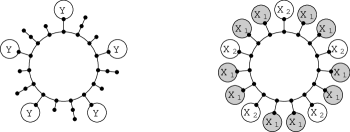
Figure 16. The construction of the described groups.

Proof of Theorem 1.4.

We first prove that ${\rm Aut(\text{\rm connected}\ \hbox{\rm CIRCLE})}$ contains all described groups. Let $G\in\Sigma$ and let $Y$ be a connected circle graph with ${\rm Stab}_{Y}(y)\cong G$. We take $n$ copies of $Y$ and attach them by $y$ to the graph depicted in Fig. 16 on the left. Clearly, we get ${\rm Aut}(x)\cong G^{n}\rtimes\mathbb{Z}_{n}$. Let $G_{1},G_{2}\in\Sigma$ and let $X_{1}$ and $X_{2}$ be connected circle graphs such that ${\rm Stab}_{X_{i}}(x_{i})\cong G_{i}$ and $X_{1}\not\cong X_{2}$. We construct a graph $X$ by attaching $n$ copies of $X_{1}$ by $x_{1}$ and $2n$ copies of $X_{2}$ by $x_{2}$ as in Fig. 16 on the right. We get ${\rm Aut}(X)\cong(G_{1}^{n}\times G_{2}^{2n})\rtimes\mathbb{D}_{n}$.

Let $X$ be a connected circle graph, we want to show that ${\rm Aut}(X)$ can be constructed in the above way. Let $S$ be its split, by Lemma 5.2 we have ${\rm Aut}(S)\cong{\rm Aut}(X)$. For the central node $C$, we get by Lemma 5.4 that

$${\rm Aut}(S)\cong\bigl{(}{\rm Stab}_{S[N_{1}]}(m_{1})\times\cdots\times{\rm Stab}_{S[N_{k}]}(m_{k})\bigr{)}\rtimes{\rm Aut}(C),$$

where $N_{1},\dots,N_{k}$ are children of $C$ and $m_{1},\dots,m_{k}$ are their root marker vertices. By Lemma 5.7, we know that each ${\rm Stab}_{S[N_{i}]}\in\Sigma$ and also $\prod{\rm Stab}_{S[N_{i}]}(m_{i})\in\Sigma$. The rest follows by analysing the automorphism group ${\rm Aut}(C)$ and its orbits.

Case 1: $C$ is a degenerate node. This is exactly the same as Case 1 in the proof of Lemma 5.7. We get that ${\rm Aut}(S)\in\Sigma$, so it is the semidirect product with $\mathbb{Z}_{1}$.

Case 2: $C$ is a prime node. By Lemma 5.5, we know that ${\rm Aut}(C)$ is isomorphic to either $\mathbb{Z}_{n}$, or $\mathbb{D}_{n}$. If $n\leq 2$, we can show by a similar argument that ${\rm Aut}(S)\in\Sigma$.

If ${\rm Aut}(C)\cong\mathbb{Z}_{n}$, where $n\geq 3$, then by Lemma 5.5 we know that ${\rm Aut}(C)$ consists of rotations which act semiregularly. Therefore each orbit of ${\rm Aut}(C)$ is of size $n$ and ${\rm Aut}(C)$ acts isomorphically on them. Let $G\in\Sigma$ be the direct product of ${\rm Stab}_{S[N_{i}]}(m_{i})$, one for each orbit of ${\rm Aut}(C)$. It follows that

$${\rm Aut}(S)\cong G^{n}\rtimes{\rm Aut}(C)=G\wr\mathbb{Z}_{n}.$$

If ${\rm Aut}(C)\cong\mathbb{D}_{n}$, where $n\geq 3$, then by Lemma 5.5 there exists a subgroup of rotations of index two, acting semiregularly. Therefore each orbit of ${\rm Aut}(C)$ is of size $n$ or $2n$. On the orbits of size $2n$, we know that ${\rm Aut}(C)$ acts regularly. Let $\rho\in{\rm Aut}(C)$ be the basic rotation by $k$. Then the chords belonging to an orbit of size $n$ are cyclically shifted by $k$ endpoints. Therefore ${\rm Aut}(C)$ acts on all of them isomorphically, exactly as on the vertices of a regular $n$-gon. Let $G_{1}\in\Sigma$ be the direct product of ${\rm Stab}_{S[N_{i}]}(m_{i})$, one from each orbit of size $n$, and let $G_{2}\in\Sigma$ be the direct product of ${\rm Stab}_{S[N_{i}]}(m_{i})$, one for each orbit of size $2n$. We get:

$${\rm Aut}(S)\cong(G_{1}^{n}\times G_{2}^{2n})\rtimes{\rm Aut}(C)=(G_{1}^{n}\times G_{2}^{2n})\rtimes\mathbb{D}_{n},$$

where $\mathbb{D}_{n}$ permutes the coordinates in $G_{1}^{n}$ exactly as the vertices of a regular $n$-gon, and permutes the coordinates in $G_{2}^{2n}$ regularly. ∎

5.5. The Action on Circle Representations.

For a connected circle graph $X$, the set $\mathfrak{Rep}/\mathord{\sim}$ consists of all circular orderings of the endpoints of the chords which give a correct representation of $X$. Then $\pi({\mathcal{R}})$ is the representation in which the endpoints are mapped by $\pi$. The stabilizer ${\rm Aut}({\mathcal{R}})$ can only rotate/reflect this circular ordering, so it is a subgroup of a dihedral group. For prime circle graphs, we know that ${\rm Aut}({\mathcal{R}})={\rm Aut}(X)$. A general circle graph may have many different representations, and the action of ${\rm Aut}(X)$ on them may consist of several non-isomorphic orbits and ${\rm Aut}({\mathcal{R}})$ may not be a normal subgroup of ${\rm Aut}(X)$.

The above results have the following interpretation in terms of the action of ${\rm Aut}(X)$. By Lemma 5.2, we know that ${\rm Aut}(S)\cong{\rm Aut}(X)$. We assume that the center $C$ is a prime circle graph, otherwise ${\rm Aut}({\mathcal{R}})$ is very restricted ($\mathbb{Z}_{1}$ or $\mathbb{Z}_{2}$) and not very interesting. We choose a representation ${\mathcal{R}}$ belonging to the smallest orbit, i.e., ${\mathcal{R}}$ is one of the most symmetrical representations. Then ${\rm Aut}({\mathcal{R}})$ consists of the rotations/reflections of $C$ described in the proof of Theorem 1.4.

The action of ${\rm Aut}(X)$ on this orbit is described by the point-wise stabilizer $H$ of $C$ in ${\rm Aut}(S)$. We know that $H=\prod{\rm Stab}_{S[N_{i}]}(m_{i})$ as described in Lemma 5.7. When $N_{i}$ is a prime graph, we can apply reflections and rotations described in Lemma 5.6, so we get a subgroup of $\mathbb{Z}_{2}^{2}$. If $N_{i}$ is a degenerate graph, then isomorphic subtrees can be arbitrarily permuted which corresponds to permuting small identical parts of a circle representation. It follows that ${\rm Aut}(X)\cong H\rtimes{\rm Aut}({\mathcal{R}})$.

6. Automorphism Groups of Comparability and Permutation Graphs

All transitive orientations of a graph are efficiently captured by the modular decomposition which we encode into the modular tree. We study the induced action of ${\rm Aut}(X)$ on the set of all transitive orientations. We show that this action is captured by the modular tree, but for general comparability graphs its stabilizers can be arbitrary groups. In the case of permutation graphs, we study the action of ${\rm Aut}(X)$ on the pairs of orientations of the graph and its complement, and show that it is semiregular. Using this, we prove Theorem 1.5. We also show that an arbitrary graph can be encoded into a comparability graph of the dimension at most four, which establishes Theorem 1.7.

6.1. Modular Decomposition

A module $M$ of a graph $X$ is a set of vertices such that each $x\in V(X)\setminus M$ is either adjacent to all vertices in $M$, or to none of them. Modules generalize connected components, but one module can be a proper subset of another one. Therefore, modules lead to a recursive decomposition of a graph, instead of just a partition. See Fig. 17a for examples. A module $M$ is called trivial if $M=V(X)$ or $|M|=1$, and non-trivial otherwise.

If $M$ and $M^{\prime}$ are two disjoint modules, then either the edges between $M$ and $M^{\prime}$ form the complete bipartite graph, or there are no edges at all; see Fig. 17a. In the former case, $M$ and $M^{\prime}$ are called adjacent, otherwise they are non-adjacent.

Figure 17. (a) A graph $X$ with a modular partition ${\mathcal{P}}$. (b) The quotient graph $X/{\mathcal{P}}$ is prime.

Quotient Graphs. Let ${\mathcal{P}}=\{M_{1},\dots,M_{k}\}$ be a modular partition of $V(X)$, i.e., each $M_{i}$ is a module of $X$, $M_{i}\cap M_{j}=\emptyset$ for every $i\neq j$, and $M_{1}\cup\cdots\cup M_{k}=V(X)$. We define the quotient graph $X/{\mathcal{P}}$ with the vertices $m_{1},\dots,m_{k}$ corresponding to $M_{1},\dots,M_{k}$ where $m_{i}m_{j}\in E(X/{\mathcal{P}})$ if and only if $M_{i}$ and $M_{j}$ are adjacent. In other words, the quotient graph is obtained by contracting each module $M_{i}$ into the single vertex $m_{i}$; see Fig. 17b.

Modular Decomposition. To decompose $X$, we find some modular partition ${\mathcal{P}}=\{M_{1},\dots,M_{k}\}$, compute $X/{\mathcal{P}}$ and recursively decompose $X/{\mathcal{P}}$ and each $X[M_{i}]$. The recursive process terminates on prime graphs which are graphs containing only trivial modules. There might be many such decompositions for different choices of ${\mathcal{P}}$ in each step. In 1960s, Gallai [17] described the modular decomposition in which special modular partitions are chosen and which encodes all other decompositions.

The key is the following observation. Let $M$ be a module of $X$ and let $M^{\prime}\subseteq M$. Then $M^{\prime}$ is a module of $X$ if and only if it is a module of $X[M]$. A graph $X$ is called degenerate if it is $K_{n}$ or $\overline{K}_{n}$. We construct the modular decomposition of a graph $X$ in the following way, see Fig. 18a for an example:

• If $X$ is a prime or a degenerate graph, then we terminate the modular decomposition on $X$. We stop on degenerate graphs since every subset of vertices forms a module, so it is not useful to further decompose them.

• Let $X$ and $\overline{X}$ be connected graphs. Gallai [17] shows that the inclusion maximal proper subsets of $V(X)$ which are modules form a modular partition ${\mathcal{P}}$ of $V(X)$, and the quotient graph $X/{\mathcal{P}}$ is a prime graph; see Fig. 17. We recursively decompose $X[M]$ for each $M\in{\mathcal{P}}$.

• If $X$ is disconnected and $\overline{X}$ is connected, then every union of connected components is a module. Therefore the connected components form a modular partition ${\mathcal{P}}$ of $V(X)$, and the quotient graph $X/{\mathcal{P}}$ is an independent set. We recursively decompose $X[M]$ for each $M\in{\mathcal{P}}$.

• If $\overline{X}$ is disconnected and $X$ is connected, then the modular decomposition is defined in the same way on the connected components of $\overline{X}$. They form a modular partition ${\mathcal{P}}$ and the quotient graph $X/{\mathcal{P}}$ is a complete graph. We recursively decompose $X[M]$ for each $M\in{\mathcal{P}}$.

6.2. Modular Tree.

We encode the modular decomposition by the modular tree $T$, similarly as the split decomposition is captured by the split tree in Section 5. The modular tree $T$ is a graph with two types of vertices (normal and marker vertices) and two types of edges (normal and directed tree edges). The directed tree edges connect the prime and degenerate graphs encountered in the modular decomposition (as quotients and terminal graphs) into a rooted tree.

We give a recursive definition. Every modular tree has an induced subgraph called root node. If $X$ is a prime or a degenerate graph, we define $T=X$ and its root node is equal $T$. Otherwise, let ${\mathcal{P}}=\{M_{1},\dots,M_{k}\}$ be the used modular partition of $X$ and let $T_{1},\dots,T_{k}$ be the corresponding modular trees for $X[M_{1}],\dots,X[M_{k}]$. The modular tree $T$ is the disjoint union of $T_{1},\dots,T_{k}$ and of the quotient $X/{\mathcal{P}}$ with the marker vertices $m_{1},\dots,m_{k}$. To every graph $T_{i}$, we add a new marker vertex $m^{\prime}_{i}$ such that $m^{\prime}_{i}$ is adjacent exactly to the vertices of the root node of $T_{i}$. We further add a tree edge oriented from $m_{i}$ to $m^{\prime}_{i}$. For an example, see Fig. 18b.

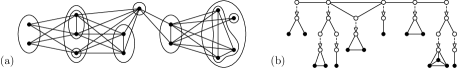
Figure 18. (a) The graph $X$ from Fig. 17 with the modular partitions used in the modular decomposition. (b) The modular tree $T$ of $X$, the marker vertices are white, the tree edges are dashed.

The modular tree of $X$ is unique. The graphs encountered in the modular decomposition are called nodes of $T$, or alternatively root nodes of some modular tree in the construction of $T$. For a node $N$, its subtree is the modular tree which has $N$ as the root node. Leaf nodes correspond to the terminal graphs in the modular decomposition, and inner nodes are the quotients in the modular decomposition. All vertices of $X$ are in leaf nodes and all marker vertices, corresponding to modules of $X$, are in inner nodes.

Similarly as in Lemma 5.1, the modular tree $T$ captures the adjacencies in $X$.

Lemma 6.1.

We have $xy\in E(X)$ if and only if there exists an alternating path $xm_{1}m_{2}\dots m_{k}y$ in the modular tree $T$ such that each $m_{i}$ is a marker vertex and precisely the edges $m_{2i-1}m_{2i}$ are tree edges.

Proof.

Both $x$ and $y$ belong to leaf nodes. If there exists an alternating path, let $N$ be the node which is the common ancestor of $x$ and $y$. This path has an edge $m_{2i}m_{2i+1}$ in $N$. These vertices correspond to adjacent modules $M_{2i}$ and $M_{2i+1}$ such that $x\in M_{2i}$ and $y\in M_{2i+1}$. Therefore $xy\in E(X)$.

On the other hand, let $N$ be the common ancestor of $x$ and $y$, such that $m_{x}$ is the marker vertex on a path from $x$ to $N$ and similarly $m_{y}$ is the marker vertex for $y$ and $N$. If $xy\in E(X)$, then the corresponding modules $M_{x}$ and $M_{y}$ has to be adjacent, so we can construct an alternating path from $x$ to $y$. ∎

6.3. Automorphisms of Modular Trees.

An automorphism of the modular tree $T$ has to preserve the types of vertices and edges and the orientation of tree edges. We denote the automorphism group of $T$ by ${\rm Aut}(T)$.

Lemma 6.2.

If $T$ is the modular tree of a graph $X$, then ${\rm Aut}(X)\cong{\rm Aut}(T)$.

Proof.

First, we show that each automorphism $\sigma\in{\rm Aut}(T)$ induces a unique automorphism of $X$. Since $V(X)\subseteq V(T)$, we define $\pi=\sigma\restriction_{V(X)}$. By Lemma 6.1, $xy\in E(X)$ if and only if there exists an alternating path in $T$ connecting them. Automorphisms preserve alternating paths, so $xy\in E(X)\iff\pi(x)\pi(y)\in E(X)$.

For the converse, we prove that $\pi\in{\rm Aut}(X)$ induces a unique automorphism $\sigma\in{\rm Aut}(T)$. We define $\sigma\restriction_{V(X)}=\pi$ and extend it recursively on the marker vertices. Let ${\mathcal{P}}=\{M_{1},\dots,M_{k}\}$ be the modular partition of $X$ used in the modular decomposition. It is easy to see that ${\rm Aut}(X)$ induces an action on ${\mathcal{P}}$. If $\pi(M_{i})=M_{j}$, then clearly $X[M_{i}]$ and $X[M_{j}]$ are isomorphic. We define $\sigma(m_{i})=m_{j}$ and $\sigma(m_{i}^{\prime})=m_{j}^{\prime}$, and finish the rest recursively. Since $\sigma$ is an automorphism at each step of the construction, it follows that $\sigma\in{\rm Aut}(T)$. ∎

Recursive Construction. We can build ${\rm Aut}(T)$ recursively. Let $N$ be the root node of $T$. Suppose that we know the automorphism groups ${\rm Aut}(T_{1}),\dots,{\rm Aut}(T_{k})$ of the subtrees $T_{1},\dots,T_{k}$ of all children of $N$. We further color the marker vertices in $N$ by colors coding isomorphism classes of the subtrees $T_{1},\dots,T_{k}$.

Lemma 6.3.

Let $N$ be the root node of $T$ with subtrees $T_{1},\dots,T_{k}$. Then

$${\rm Aut}(T)\cong\bigl{(}{\rm Aut}(T_{1})\times\cdots\times{\rm Aut}(T_{k})\bigr{)}\rtimes{\rm Aut}(N),$$

where ${\rm Aut}(N)$ is color preserving.

Proof.

Recall the proof of Theorem 2.1. We isomorphically label the vertices of the isomorphic subtrees $T_{i}$. Each automorphism $\pi\in{\rm Aut}(T)$ is a composition of two automorphisms $\sigma\cdot\tau$ where $\sigma$ maps each subtree $T_{i}$ to itself, and $\tau$ permutes the subtrees as in $\pi$ while preserving the labeling. Therefore, the automorphisms $\sigma$ can be identified with the elements of ${\rm Aut}(T_{1})\times\cdots\times{\rm Aut}(T_{k})$ and the automorphisms $\tau$ with the elements of ${\rm Aut}(N)$. The rest is exactly as in the proof of Theorem 2.1. ∎

With no further assumptions on $X$, if $N$ is a prime graph, then ${\rm Aut}(N)$ can be isomorphic to an arbitrary group, as shown in Section 6.7. If $N$ is a degenerate graph, then ${\rm Aut}(N)$ is a direct product of symmetric groups.

Automorphism Groups of Interval Graphs. In Section 4, we proved using MPQ-trees that ${\rm Aut}(\hbox{\rm INT})={\rm Aut}(\hbox{\rm TREE})$. The modular decomposition gives an alternative derivation that ${\rm Aut}(\hbox{\rm INT})\subseteq{\rm Aut}(\hbox{\rm TREE})$ by Lemma 6.3 and the following:

Lemma 6.4.

For a prime interval graph $X$, ${\rm Aut}(X)$ is a subgroup of $\mathbb{Z}_{2}$.

Proof.

Hsu [25] proved that prime interval graphs have exactly two consecutive orderings of the maximal cliques. Since $X$ has no twin vertices, ${\rm Aut}(X)$ acts semiregularly on the consecutive orderings and there is at most one non-trivial automorphism in ${\rm Aut}(X)$. ∎

6.4. Automorphism Groups of Comparability Graphs

In this section, we explain the structure of the automorphism groups of comparability graphs, in terms of actions on sets of transitive orientations.

Structure of Transitive Orientations. Let $\to$ be a transitive orientation of $X$ and let $T$ be the modular tree. For modules $M_{1}$ and $M_{2}$, we write $M_{1}\to M_{2}$ if $x_{1}\to x_{2}$ for all $x_{1}\in M_{1}$ and $x_{2}\in M_{2}$. Gallai [17] shows the following properties. If $M_{1}$ and $M_{2}$ are adjacent modules of a partition used in the modular decomposition, then either $M_{1}\to M_{2}$, or $M_{1}\leftarrow M_{2}$. The graph $X$ is a comparability graph if and only if each node of $T$ is a comparability graph. Every prime comparability graph has exactly two transitive orientations, one being the reversal of the other.

The modular tree $T$ encodes all transitive orientations as follows. For each prime node of $T$, we arbitrarily choose one of the two possible orientations. For each degenerate node, we choose some orientation. (Where $K_{n}$ has $n!$ possible orientations and $\overline{K_{n}}$ has the unique orientation.) A transitive orientation of $X$ is then constructed as follows. We orient the edges of leaf nodes as above. For a node $N$ partitioned in the modular decomposition by ${\mathcal{P}}=\{M_{1},\dots,M_{k}\}$, we orient $X[M_{i}]\to X[M_{j}]$ if and only if $m_{i}\to m_{j}$ in $N$. It is easy to check that this gives a valid transitive orientation, and every transitive orientation can be constructed by some orientation of the nodes of $T$. We note that this implies that the dimension of the transitive orientation is the maximum of the dimensions over all nodes of $T$, and that this dimension is the same for every transitive orientation.

Action Induced On Transitive Orientations. Let $\mathfrak{to}(X)$ be the set of all transitive orientations of $X$. Let $\pi\in{\rm Aut}(X)$ and $\mathord{\to}\in\mathfrak{to}(X)$. We define the orientation $\pi(\mathord{\to})$ as follows:

$$x\to y\implies\pi(x)\mathrel{\pi(\mathord{\to})}\pi(y),\qquad\forall x,y\in V(X).$$

We can observe that $\pi(\mathord{\to})$ is a transitive orientation of $X$, so $\pi(\mathord{\to})\in\mathfrak{to}(X)$; see Fig. 19. It easily follows that ${\rm Aut}(X)$ defines an action on $\mathfrak{to}(X)$.

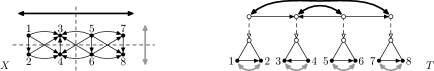
Figure 19. Two automorphisms reflect $X$ and change the transitive orientation, and their action on the modular tree $T$.

Let ${\rm Stab}(\mathord{\to})$ be the stabilizer of some orientation $\mathord{\to}\in\mathfrak{to}(X)$. It consists of all automorphisms which preserve this orientation, so only the vertices that are incomparable in $\mathord{\to}$ can be permuted. In other words, ${\rm Stab}(\mathord{\to})$ is the automorphism group of the poset created from the transitive orientation $\mathord{\to}$ of $X$. Since posets are universal [3, 41], ${\rm Stab}(\mathord{\to})$ can be arbitrary groups and in general the structure of ${\rm Aut}(X)$ cannot be derived from its action on $\mathfrak{to}(X)$, which is not faithful enough.

Lemma 6.3 allows to understand it in terms of ${\rm Aut}(T)$ for the modular tree $T$ representing $X$. Each automorphism of ${\rm Aut}(T)$ somehow acts inside each node, and somehow permutes the attached subtrees. Consider a node $N$ with attached subtrees $T_{1},\dots,T_{k}$. If $\sigma\in{\rm Stab}(\mathord{\to})$, then it preserves the orientation in $N$. Therefore if it maps $T_{i}$ to $\sigma(T_{i})$, the corresponding marker vertices are necessarily incomparable in $N$. If $N$ is an independent set, the isomorphic subtrees can be arbitrarily permuted in ${\rm Stab}(\mathord{\to})$. If $N$ is a complete graph, all subtrees are preserved in ${\rm Stab}(\mathord{\to})$. If $N$ is a prime graph, then isomorphic subtrees of incomparable marker vertices can be permuted according to the structure of $N$ which can be complex.

It is easy to observe that stabilizers of all orientations are the same and that ${\rm Stab}(\mathord{\to})$ is a normal subgroup. Let $H={\rm Aut}(X)/{\rm Stab}(\mathord{\to})$, so $H$ captures the action of ${\rm Aut}(X)$ on $\mathfrak{to}(X)$. This quotient group can be constructed recursively from the structure of $T$, similarly to Lemma 6.3. Suppose that we know $H_{1},\dots,H_{k}$ of the subtrees $T_{1},\dots,T_{k}$. If $N$ is an independent set, there is exactly one transitive orientation, so $H\cong H_{1}\times\cdots\times H_{k}$. If $N$ is a complete graph, isomorphic subtrees can be arbitrarily permuted, so $H$ can be constructed exactly as in Theorem 2.1. If $N$ is a prime node, there are exactly two transitive orientations. If there exists an automorphism changing the orientation of $N$, we can describe $H$ by a semidirect product with $\mathbb{Z}_{2}$ as in Theorem 2.1. And if $N$ is asymmetric, then $H\cong H_{1}\times\cdots\times H_{k}$. In particular, this description implies that $H\in{\rm Aut}(\hbox{\rm TREE})$.

6.5. Automorphism Groups of Permutation Graphs

In this section, we derive the characterization of ${\rm Aut}(\hbox{\rm PERM})$ stated in Theorem 1.5.

Action Induced On Pairs of Transitive Orientations. Let $X$ be a permutation graph. In comparison to general comparability graphs, the main difference is that both $X$ and $\overline{X}$ are comparability graphs. From the results of Section 6.4 it follows that ${\rm Aut}(X)$ induces an action on both $\mathfrak{to}(X)$ and $\mathfrak{to}(\overline{X})$. Let $\mathfrak{to}(X,\overline{X})=\mathfrak{to}(X)\times\mathfrak{to}(\overline{X})$, and we work with one action on the pairs $(\mathord{\to},\overline{\raisebox{0.0pt}[4.97922pt]{$\mathord{\to}$}})\in\mathfrak{to}(X,\overline{X})$. Figure 20 shows an example.

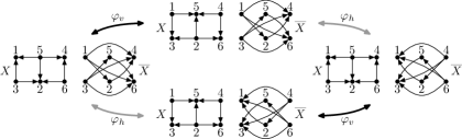
Figure 20. The action of ${\rm Aut}(X)$ on four pairs of transitive orientations $X$. The black generator flips the orientation of $X$, the gray automorphism of both $X$ and $\overline{X}$.

Lemma 6.5.

For a permutation graph $X$, the action of ${\rm Aut}(X)$ on $\mathfrak{to}(X,\overline{X})$ is semiregular.

Proof.

Since a permutation belonging to the stabilizer of $(\mathord{\to},\overline{\raisebox{0.0pt}[4.97922pt]{$\mathord{\to}$}})$ fixes both orientations, it can only permute incomparable elements. But incomparable elements in $\mathord{\to}$ are exactly the comparable elements in $\overline{\raisebox{0.0pt}[4.97922pt]{$\mathord{\to}$}}$, so the stabilizer is trivial. ∎

Lemma 6.6.

For a prime permutation graph $X$, ${\rm Aut}(X)$ is a subgroup of $\mathbb{Z}_{2}^{2}$.

Proof.

There are at most four pairs of orientations in $\mathfrak{to}(X,\overline{X})$, so by Lemma 6.5 the order of ${\rm Aut}(X)$ is at most four. If $\pi\in{\rm Aut}(X)$, then $\pi^{2}$ fixes the orientations of both $X$ and $\overline{X}$. Therefore $\pi^{2}$ belongs to the stabilizers and it is an identity. Thus $\pi$ is the involution and ${\rm Aut}(X)$ is a subgroup of $\mathbb{Z}_{2}^{2}$. ∎

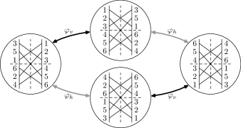
Figure 21. Four representations of a symmetric permutation graph. The black automorphism is the horizontal reflection, the gray automorphism is the vertical reflection.

Geometric Interpretation. First, we explain the result $\hbox{\rm PERM}=\hbox{\rm$2$-DIM}$ of Even et al. [13]. Let $\mathord{\to}\in\mathfrak{to}(X)$ and $\overline{\raisebox{0.0pt}[4.97922pt]{$\mathord{\to}$}}\in\mathfrak{to}(\overline{X})$, and let $\overline{\raisebox{0.0pt}[4.97922pt]{$\mathord{\to}$}}_{R}$ be the reversal of $\overline{\raisebox{0.0pt}[4.97922pt]{$\mathord{\to}$}}$. We construct two linear orderings $L_{1}=\mathord{\to}\cup\overline{\raisebox{0.0pt}[4.97922pt]{$\mathord{\to}$}}$ and $L_{2}=\mathord{\to}\cup\overline{\raisebox{0.0pt}[4.97922pt]{$\mathord{\to}$}}_{R}$. The comparable pairs in $L_{1}\cap L_{2}$ are precisely the edges $E(X)$.

Consider a permutation representation of a symmetric prime permutation graph. The vertical reflection $\varphi_{v}$ corresponds to exchanging $L_{1}$ and $L_{2}$, which is equivalent to reversing $\overline{\raisebox{0.0pt}[4.97922pt]{$\mathord{\to}$}}$. The horizontal reflection $\varphi_{h}$ corresponds to reversing both $L_{1}$ and $L_{2}$, which is equivalent to reversing both $\mathord{\to}$ and $\overline{\raisebox{0.0pt}[4.97922pt]{$\mathord{\to}$}}$. We denote the central $180^{\circ}$ rotation by $\rho=\varphi_{h}\cdot\varphi_{v}$ which corresponds to reversing $\mathord{\to}$; see Fig. 21.

The Inductive Characterization. Now, we are ready to prove Theorem 1.5.

Proof of Theorem 1.5.

First, we show that ${\rm Aut}(\hbox{\rm PERM})$ is closed under (b) to (d). For (b), let $G_{1},G_{2}\in{\rm Aut}(\hbox{\rm PERM})$, and let $X_{1}$ and $X_{2}$ be two permutation graphs such that ${\rm Aut}(X_{i})\cong G_{i}$. We construct $X$ by attaching $X_{1}$ and $X_{2}$ as in Fig. 22b. Clearly, ${\rm Aut}(X)\cong G_{1}\times G_{2}$. For (c), let $G\in{\rm Aut}(\hbox{\rm PERM})$ and let $Y$ be a connected permutation graph such that ${\rm Aut}(Y)\cong G$. We construct $X$ as the disjoint union of $n$ copies of $Y$; see Fig. 22c. We get ${\rm Aut}(X)\cong G\wr\mathbb{S}_{n}$. Let $G_{1},G_{2},G_{3}\in{\rm Aut}(\hbox{\rm PERM})$, and let $X_{1}$, $X_{2}$, and $X_{3}$ be permutation graphs such that ${\rm Aut}(X_{i})\cong G_{i}$. We construct $X$ as in Fig. 22d. We get ${\rm Aut}(X)\cong\bigl{(}G_{1}^{4}\times G_{2}^{2}\times G_{3}^{2}\bigr{)}\rtimes\mathbb{Z}_{2}^{2}$.

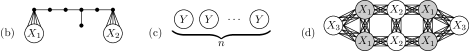
Figure 22. The constructions in the proof of Theorem 1.5.

We show the other implication by induction. Let $X$ be a permutation graph and let $T$ be the modular tree representing $X$. By Lemma 6.2, we know that ${\rm Aut}(T)\cong{\rm Aut}(X)$. Let $N$ be the root node of $T$, and let $T_{1},\dots,T_{k}$ be the subtrees attached to $N$. By the induction hypothesis, we assume that ${\rm Aut}(T_{i})\in{\rm Aut}(\hbox{\rm PERM})$. By Lemma 6.3,

$${\rm Aut}(T)\cong\bigl{(}{\rm Aut}(T_{1})\times\cdots\times{\rm Aut}(T_{k})\bigr{)}\rtimes{\rm Aut}(N).$$

Case 1: $N$ is a degenerate node. Then ${\rm Aut}(N)$ is a direct product of symmetric groups. The subtrees attached to marker vertices of each color class can be arbitrarily permuted, independently of each other. Therefore ${\rm Aut}(T)$ can be constructed using (b) and (c), exactly as in Theorem 2.1.

Case 2: $N$ is a prime node. By Lemma 6.6, ${\rm Aut}(N)$ is a subgroup of $\mathbb{Z}_{2}^{2}$. If it is trivial or $\mathbb{Z}_{2}$, observe that it can be constructed using (b) and (c). The only remaining case is when ${\rm Aut}(N)\cong\mathbb{Z}_{2}^{2}$. The action of $\mathbb{Z}_{2}^{2}$ on $V(N)$ can have orbits of sizes $4$, $2$, and $1$. By Orbit-Stabilizer Theorem, each orbit of size $2$ has also a stabilizer of size $2$, having exactly one non-trivial element. Therefore, there are at most three types of orbits of size $2$, according to which element of $\mathbb{Z}_{2}^{2}$ stabilizes them. We give a geometric argument that one of these elements cannot be a stabilizer of an orbit of size $2$, so there are at most two types of orbits of size $2$.

As argued above, the non-identity elements of $\mathbb{Z}_{2}^{2}$ correspond geometrically to the reflections $\varphi_{v}$ and $\varphi_{h}$ and to the rotation $\rho$; see Fig. 21. The reflection $\varphi_{v}$ stabilizes those segments which are parallel to the horizontal axis. The rotation $\rho$ stabilizes those segments which cross the central point. For both automorphisms, there might be multiple segments stabilized. On the other hand, the reflection $\varphi_{h}$ stabilizes at most one segment which lies on the axis of $\varphi_{h}$. Further, this segment is stabilized by all elements of $\mathbb{Z}_{2}^{2}$, so it belongs to the orbit of size $1$. Therefore, there exists no orbit of size $2$ which is stabilized by $\varphi_{h}$.

Let $G_{1}$ be the direct product of all ${\rm Aut}(T_{j})$, one for each orbit of size four. The groups $G_{2}$ and $G_{3}$ are defined similarly for the orbits of size two stabilized by $\varphi_{v}$ and $\rho$, respectively, and $G_{4}$ for the orbit of size one (if it exists). We have

$${\rm Aut}(T)\cong\bigl{(}G_{1}^{4}\times G_{2}^{2}\times G_{3}^{2}\bigr{)}\rtimes_{\psi}\mathbb{Z}_{2}^{2}\times G_{4},$$

where $\psi(\varphi_{h})$ and $\psi(\varphi_{v})$ swap the coordinates as $\varphi_{h}$ and $\varphi_{v}$ in Fig. 21. So ${\rm Aut}(T)$ can be constructed using (b) and (d). ∎

6.6. Automorphism Groups of Bipartite Permutation Graphs.

We use the modular trees to characterize ${\rm Aut}({\rm connected}\ \hbox{\rm BIP PERM})$. For a connected bipartite graph, every non-trivial module is an independent set, and the quotient is a prime bipartite permutation graph. Therefore, the modular tree $T$ has a prime root node $N$, to which there are attached leaf nodes which are independent sets.

Figure 23. Let $G_{1}=\mathbb{S}_{k_{1}}\times\cdots\times\mathbb{S}_{k_{\ell}}$, $G_{2}=\mathbb{S}_{n}$ and $G_{3}=\mathbb{S}_{m}$. The constructed graphs consist of independent sets joined by complete bipartite subgraphs. They have the following automorphism groups: (a) $G_{1}$, (b) $G_{1}\wr\mathbb{Z}_{2}\times G_{2}\times G_{3}$, (c) $(G_{1}^{4}\times G_{2}^{2})\rtimes\mathbb{Z}_{2}^{2}$.

Proof of Corollary 1.6.

Every abstract group from Corollary 1.6 can be constructed as shown in Fig. 23. Let $T$ be the modular tree representing $X$. By Lemmas 6.2 and 6.3,

$${\rm Aut}(X)\cong\bigl{(}{\rm Aut}(T_{1})\times\cdots\times{\rm Aut}(T_{k})\bigr{)}\rtimes{\rm Aut}(N),$$

where ${\rm Aut}(N)$ is isomorphic to a subgroup of $\mathbb{Z}_{2}^{2}$ (by Lemma 6.6), and each ${\rm Aut}(T_{i})$ is a symmetric group since $T_{i}$ is an independent set.

Consider a permutation representation of $N$ in which the endpoints of the segments, representing $V(N)$, are placed equidistantly as in Fig. 21. By [36], there are no segments parallel with the horizontal axis, so the reflections $\varphi_{v}$ and $\varphi_{h}$ fix no segment. Further, since $N$ is bipartite, there are at most two segments crossing the central point, so the rotation $\rho$ can fix at most two segments.

Case 1: ${\rm Aut}(N)$ is trivial. Then ${\rm Aut}(X)$ is a direct product of symmetric groups.

Case 2: ${\rm Aut}(N)\cong\mathbb{Z}_{2}$. Let $G_{1}$ be the direct product of all ${\rm Aut}(T_{i})$, one for each orbit of size two. Notice that ${\rm Aut}(N)$ is generated by exactly one of $\varphi_{v}$, $\varphi_{h}$, and $\rho$. For $\varphi_{v}$ or $\varphi_{h}$, all orbits are of size two, so ${\rm Aut}(X)\cong G_{1}\wr\mathbb{Z}_{2}$. For $\rho$, there are at most two fixed segments, so ${\rm Aut}(X)\cong G_{1}\wr\mathbb{Z}_{2}\times G_{2}\times G_{3}$, where $G_{2}$ and $G_{3}$ are isomorphic to ${\rm Aut}(T_{i})$, for each of two orbits of size one.

Case 3: ${\rm Aut}(N)\cong\mathbb{Z}_{2}^{2}$. Then ${\rm Aut}(N)$ has no orbits of size $1$, at most one of size $2$, and all other of size $4$. Let $G_{1}$ be the direct product of all ${\rm Aut}(T_{i})$, one for each orbit of size $4$, and let $G_{2}$ be ${\rm Aut}(T_{i})$ for the orbit of size $2$. We have ${\rm Aut}(X)\cong(G_{1}^{4}\times G_{2}^{2})\rtimes_{\psi}\mathbb{Z}_{2}^{2}$, where $\psi$ is defined in the proof of Theorem 1.5. ∎

6.7. $k$-Dimensional Comparability Graphs

In this section, we prove that ${\rm Aut}(\hbox{\rm$4$-DIM})$ contains all abstract finite groups, i.e., each finite group can be realised as an automorphism group of some $4$-dimensional comparability graph. Our construction also shows that graph isomorphism testing of $4$-DIM is GI-complete. Both results easily translate to $k$-DIM for $k>4$ since $\hbox{\rm$4$-DIM}\subsetneq\hbox{\rm$k$-DIM}$.

The Construction. Let $X$ be a graph with $V(X)=\{x_{1},\dots,x_{n}\}$ and $E(X)=\{e_{1},\dots,e_{m}\}$. We define

$$P=\bigl{\{}p_{i}:x_{i}\in V(X)\bigr{\}},\qquad Q=\{q_{ik}:x_{i}\in e_{k}\},\qquad R=\bigl{\{}r_{k}:e_{k}\in E(X)\bigr{\}},$$

where $P$ represents the vertices, $R$ represents the edges and $Q$ represents the incidences between the vertices and the edges.

The constructed comparability graph $C_{X}$ is defined as follows, see Fig. 24:

$$V(C_{X})=P\cup Q\cup R,\qquad E(C_{X})=\{p_{i}q_{ik},q_{ik}r_{k}:x_{i}\in e_{k}\}.$$

So $C_{X}$ is created from $X$ by replacing each edge with a path of length four.

Figure 24. The construction $C_{X}$ for the graph $X=K_{2,3}$.

Lemma 6.7.

For a connected graph $X\not\cong C_{n}$, ${\rm Aut}(C_{X})\cong{\rm Aut}(X)$.∎

Lemma 6.8.

If $X$ is a connected bipartite graph, then ${\rm dim}(C_{X})\leq 4$.

Proof.

We construct four chains such that $L_{1}\cap L_{2}\cap L_{3}\cap L_{4}$ have two vertices comparable if and only if they are adjacent in $C_{X}$. We describe linear chains as words containing each vertex of $V(C_{X})$ exactly once. If $S_{1},\dots,S_{s}$ is a sequence of words, the symbol $\langle S_{t}:\mathop{\uparrow}t\rangle$ is the concatenation $S_{1}S_{2}\dots S_{s}$ and $\langle S_{t}:\mathop{\downarrow}t\rangle$ is the concatenation $S_{s}S_{s-1}\dots S_{1}$. When an arrow is omitted, as in $\langle S_{t}\rangle$, we concatenate in an arbitrary order.

First, we define the incidence string $I_{i}$ which codes $p_{i}$ and its neighbors $q_{ik}$:

$$I_{i}=p_{i}\bigl{\langle}q_{ik}:p_{i}q_{ik}\in E(C_{X})\bigr{\rangle}.$$

Notice that the concatenation $I_{i}I_{j}$ contains the right edges but it further contains edges going from $p_{i}$ and $q_{ik}$ to $p_{j}$ and $q_{j\ell}$. We remove these edges by the concatenation $I_{j}I_{i}$ in some other chain.

Since $X$ is bipartite, let $(A,B)$ be the partition of its vertices. We define

$$P_{A}=\{p_{i}:x_{i}\in A\},\hskip 2.5pt \qquad Q_{A}=\{q_{ik}:x_{i}\in A\},$$

$$P_{B}=\{p_{j}:x_{j}\in B\}, \qquad Q_{B}=\{q_{jk}:x_{j}\in B\}.$$

Each vertex $r_{k}$ has exactly one neighbor in $Q_{A}$ and exactly one in $Q_{B}$.

We construct the four chains as follows:

$$L_{1} = \langle p_{i}:p_{i}\in P_{A}\rangle\langle r_{k}q_{ik}:q_{ik}\in Q_{A},\mathop{\uparrow}k\rangle\langle I_{j}:p_{j}\in P_{B},\mathop{\uparrow}j\rangle,$$

$$L_{2} = \langle p_{i}:p_{i}\in P_{A}\rangle\langle r_{k}q_{ik}:q_{ik}\in Q_{A},\mathop{\downarrow}k\rangle\langle I_{j}:p_{j}\in P_{B},\mathop{\downarrow}j\rangle,$$

$$L_{3} = \langle p_{j}:p_{j}\in P_{B}\rangle\langle r_{k}q_{jk}:q_{jk}\in Q_{B},\mathop{\uparrow}k\rangle\langle I_{i}:p_{i}\in P_{A},\mathop{\uparrow}i\rangle,$$

$$L_{4} = \langle p_{j}:p_{j}\in P_{B}\rangle\langle r_{k}q_{jk}:q_{jk}\in Q_{B},\mathop{\downarrow}k\rangle\langle I_{i}:p_{i}\in P_{A},\mathop{\downarrow}i\rangle.$$

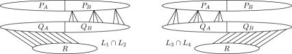
Figure 25. The forced edges in $L_{1}\cap L_{2}$ and $L_{3}\cap L_{4}$.

The four defined chains have the following properties, see Fig. 25:

• The intersection $L_{1}\cap L_{2}$ forces the correct edges between $Q_{A}$ and $R$ and between $P_{B}$ and $Q_{B}$. It poses no restrictions between $Q_{B}$ and $R$ and between $P_{A}$ and the rest of the graph.

• Similarly the intersection $L_{3}\cap L_{4}$ forces the correct edges between $Q_{B}$ and $R$ and between $P_{A}$ and $Q_{A}$. It poses no restrictions between $Q_{A}$ and $R$ and between $P_{B}$ and the rest of the graph.

It is routine to verify that the intersection $L_{1}\cap L_{2}\cap L_{3}\cap L_{4}$ is correct.

Claim 1: The edges in $Q\cup R$ are correct. For every $k$, we get $r_{k}$ adjacent to both $q_{ik}$ and $q_{jk}$ since it appear on the left in $L_{1},\dots,L_{4}$. On the other hand, $q_{ik}q_{jk}\notin E(C_{X})$ since they are ordered differently in $L_{1}$ and $L_{3}$.

For every $k<\ell$, there are no edges between $N[r_{k}]=\{r_{k},q_{ik},q_{jk}\}$ and $N[r_{\ell}]=\{r_{\ell},q_{s\ell},q_{t\ell}\}$. This can be shown by checking the four orderings of these six elements:

$$\text{in $L_{1}$:}\quad r_{k}q_{ik}\,\boxed{r_{\ell}q_{s\ell}}\,q_{jk}\,\boxed{q_{t\ell}},\quad \quad\text{in $L_{2}$:}\quad\boxed{r_{\ell}q_{s\ell}}\,r_{k}q_{ik}q_{jk}\,\boxed{q_{t\ell}},$$

$$\text{in $L_{3}$:}\quad r_{k}q_{jk}\,\boxed{r_{\ell}q_{t\ell}}\,q_{ik}\,\boxed{q_{s\ell}},\quad \quad\text{in $L_{4}$:}\quad\boxed{r_{\ell}q_{t\ell}}\,r_{k}q_{jk}q_{ik}\,\boxed{q_{s\ell}},$$

where the elements of $N[r_{\ell}]$ are boxed. $\diamond$

Claim 2: The edges in $P$ are correct. We show that there are no edges between $p_{i}$ and $p_{j}$ for $i\neq j$ as follows. If both belong to $P_{A}$ (respectively, $P_{B}$), then they are ordered differently in $L_{3}$ and $L_{4}$ (respectively, $L_{1}$ and $L_{2}$). If one belongs to $P_{A}$ and the other one to $P_{B}$, then they are ordered differently in $L_{1}$ and $L_{3}$. $\diamond$

Claim 3: The edges between $P$ and $Q\cup R$ are correct. For every $p_{i}\in P$ and $r_{k}\in R$, we have $p_{i}r_{k}\notin E(C_{X})$ because they are ordered differently in $L_{1}$ and $L_{3}$. On the other hand, $p_{i}q_{ik}\in E(C_{X})$, because $p_{i}$ is before $q_{ik}$ in $I_{i}$, and for $p_{i}\in P_{A}$ in $L_{1}$ and $L_{2}$, and for $p_{i}\in P_{B}$ in $L_{3}$ and $L_{4}$.

It remains to show that $p_{i}q_{jk}\notin E(C_{X})$ for $i\neq j$. If both $p_{i}$ and $p_{j}$ belong to $P_{A}$ (respectively, $P_{B}$), then $p_{i}$ and $q_{jk}$ are ordered differently in $L_{3}$ and $L_{4}$ (respectively, $L_{1}$ and $L_{2}$). And if one belongs to $P_{A}$ and the other one to $P_{B}$, then $p_{i}$ and $q_{jk}$ are ordered differently in $L_{1}$ and $L_{3}$. $\diamond$

These three established claims show that comparable pairs in the intersection $L_{1}\cap L_{2}\cap L_{3}\cap L_{4}$ are exactly the edges of $C_{X}$, so $C_{X}\in\hbox{\rm$4$-DIM}$. ∎

Universality of $\boldsymbol{k}$-DIM. We are ready to prove Theorem 1.7.

Proof of Theorem 1.7.

We prove the statement for $4$-DIM. Let $X$ be a connected graph such that $X\not\cong C_{n}$. First, we construct the bipartite incidence graph $Y$ between $V(X)$ and $E(X)$. Next, we construct $C_{Y}$ from $Y$. From Lemma 6.7 it follows that ${\rm Aut}(C_{Y})\cong{\rm Aut}(Y)\cong{\rm Aut}(X)$ and by Lemma 6.8, we have that $C_{Y}\in\hbox{\rm$4$-DIM}$. Similarly, if two graphs $X_{1}$ and $X_{2}$ are given, we construct $C_{Y_{1}}$ and $C_{Y_{2}}$ such that $X_{1}\cong X_{2}$ if and only if $C_{Y_{1}}\cong C_{Y_{2}}$; this polynomial-time reduction shows GI-completeness of graph isomorphism testing.

The constructed graph $C_{Y}$ is a prime graph. We fix the transitive orientation in which $P$ and $R$ are the minimal elements and get the poset $P_{Y}$ with ${\rm Aut}(P_{Y})\cong{\rm Aut}(C_{Y})$. Hence, our results translate to posets of the dimension at most four. ∎

7. Algorithms for Computing Automorphism Groups

Using PQ-trees, Colbourn and Booth [8] give a linear-time algorithm to compute permutation generators of the automorphism group of an interval graph. We are not aware of any such algorithm for circle and permutation graphs, but some of our results might be known from the study of graph isomorphism problem [25, 7].

We briefly explain algorithmic implications of our results which allow to compute automorphism groups of studied classes in terms of $\mathbb{Z}_{n}$, $\mathbb{D}_{n}$ and $\mathbb{S}_{n}$, and their group products. This description is better than just a list of permutations generating ${\rm Aut}(X)$. Many tools of the computational group theory are devoted to getting better understanding of an unknown group. Our description gives this structural understanding of ${\rm Aut}(X)$ for free.

For interval graphs, we get a linear-time algorithm by computing an MPQ-tree [29] and finding its symmetries. For circle graphs, our description easily leads to a polynomial-time algorithm, by computing the split tree for each connected component and understanding its symmetries. The best algorithm for computing split trees runs in almost linear time [19]. For permutation graph, we get a linear-time algorithm by computing the modular decomposition [33] and finding symmetries of prime permutation graphs.

8. Open Problems

We conclude this paper with several open problems concerning automorphism groups of other intersection-defined classes of graphs; for an overview see [20, 39].

Circular-arc graphs (CIRCULAR-ARC) are intersection graphs of circular arcs and they naturally generalize interval graphs. Surprisingly, this class is very complex and quite different from interval graphs. Hsu [25] relates them to circle graphs.

Problem 1.

What is ${\rm Aut}(\hbox{\rm CIRCULAR-ARC})$?

Let $Y$ be any fixed graph. The class $Y$-GRAPH consists of all intersections graphs of connected subgraphs of a subdivision of $Y$. Observe that $\hbox{\rm$K_{2}$-GRAPH}=\hbox{\rm INT}$ and we have an infinite hierarchy between INT and CHOR is formed by $T$-GRAPH for a tree $T$, for which $\hbox{\rm INT}\subseteq\hbox{\rm$T$-GRAPH}\subsetneq\hbox{\rm CHOR}$. If $Y$ contains a cycle, then $\hbox{\rm$Y$-GRAPH}\not\subseteq\hbox{\rm CHOR}$. For instance, $\hbox{\rm$K_{3}$-GRAPH}=\hbox{\rm CIRCULAR-ARC}$.

Conjecture 1.

For every fixed graph $Y$, the class $Y$-GRAPH is non-universal.

The last open problem involves the open case of $3$-DIM.

Conjecture 2.

The class $3$-DIM is universal and its graph isomorphism problem is GI-complete.

Acknowlegment. We would like to thank to Roman Nedela for many comments. A part of this work was done during a visit at Matej Bel University.

References

- [1] L. Babai, Automorphism groups of planar graphs II, Infinite and finite sets (Proc. Conf. Kestzthely, Hungary), 1973.
- [2] K. A. Baker, P. C. Fishburn, and F. S. Roberts, Partial orders of dimension 2, Networks 2 (1972), 11–28.
- [3] G. Birkhoff, On groups of automorphisms, Rev. Un. Mat. Argentina 11 (1946), 155–157.
- [4] K. S. Booth and G. S. Lueker, Testing for the consecutive ones property, interval graphs, and planarity using PQ-tree algorithms, J. Comput. System Sci. 13 (1976), 335–379.
- [5] N. Carter, Visual group theory, MAA, 2009.
- [6] S. Chaplick, S. Felsner, U. Hoffmann, and V. Wiechert, Grid intersection graphs and order dimension, In preparation.
- [7] C. J. Colbourn, On testing isomorphism of permutation graphs, Networks 11 (1981), no. 1, 13–21.
- [8] C. J. Colbourn and K. S. Booth, Linear times automorphism algorithms for trees, interval graphs, and planar graphs, SIAM J. Comput. 10 (1981), no. 1, 203–225.
- [9] D. G. Corneil, H. Kim, S. Natarajan, S. Olariu, and A. P. Sprague, Simple linear time recognition of unit interval graphs, Information Processing Letters 55 (1995), no. 2, 99–104.
- [10] W.H. Cunningham, Decomposition of directed graphs, SIAM Journal on Algebraic Discrete Methods 3 (1982), 214–228.
- [11] B. Dushnik and E. W. Miller, Partially ordered sets, American Journal of Mathematics 63 (1941), no. 3, 600–610.
- [12] P. Erdős and A. Rényi, Asymmetric graphs, Acta Mathematica Academiae Scientiarum Hungarica 14 (1963), no. 3–4, 295–315.
- [13] S. Even, A. Pnueli, and A. Lempel, Permutation graphs and transitive graphs, Journal of the ACM (JACM) 19 (1972), no. 3, 400–410.
- [14] R. Frucht, Herstellung von graphen mit vorgegebener abstrakter gruppe, Compositio Mathematica 6 (1939), 239–250.
- [15] D. R. Fulkerson and O. A. Gross, Incidence matrices and interval graphs., Pac. J. Math. 15 (1965), 835–855.
- [16] C. P. Gabor, K. J. Supowit, and W.-L. Hsu, Recognizing circle graphs in polynomial time, Journal of the ACM (JACM) 36 (1989), no. 3, 435–473.
- [17] T. Gallai, Transitiv orientierbare graphen, Acta Math. Hungar. 18 (1967), no. 1, 25–66.
- [18] E. Gioan and C. Paul, Split decomposition and graph-labelled trees: Characterizations and fully dynamic algorithms for totally decomposable graphs, Discrete Appl. Math. 160 (2012), no. 6, 708–733.
- [19] E. Gioan, C. Paul, M. Tedder, and D. Corneil, Practical and efficient circle graph recognition, Algorithmica (2013), 1–30.
- [20] M. C. Golumbic, Algorithmic graph theory and perfect graphs, vol. 57, Elsevier, 2004.
- [21] M. C. Golumbic, D. Rotem, and J. Urrutia, Comparability graphs and intersection graphs, Discrete Mathematics 43 (1983), no. 1, 37–46.
- [22] M. Grohe and D. Marx, Structure theorem and isomorphism test for graphs with excluded topological subgraphs, Proceedings of the Forty-fourth Annual ACM Symposium on Theory of Computing, STOC ’12, 2012, pp. 173–192.
- [23] P. Hanlon, Counting interval graphs, Transactions of the American Mathematical Society 272 (1982), no. 2, 383–426.
- [24] Z. Hedrlín, A. Pultr, et al., On full embeddings of categories of algebras, Illinois Journal of Mathematics 10 (1966), no. 3, 392–406.
- [25] W. L. Hsu, algorithms for the recognition and isomorphism problems on circular-arc graphs, SIAM Journal on Computing 24 (1995), no. 3, 411–439.
- [26] C. Jordan, Sur les assemblages de lignes., Journal für die reine und angewandte Mathematik 70 (1869), 185–190.
- [27] P. Klavík and R. Nedela, Automorphism groups of planar graphs, In preparation (2015).
- [28] P. Klavík and P. Zeman, Automorphism groups of geometrically represented graphs, 32nd International Symposium on Theoretical Aspects of Computer Science (STACS 2015), Leibniz International Proceedings in Informatics (LIPIcs), vol. 30, 2015, pp. 540–553.
- [29] N. Korte and R. H. Möhring, An incremental linear-time algorithm for recognizing interval graphs, SIAM J. Comput. 18 (1989), no. 1, 68–81.
- [30] G. S. Lueker and K. S. Booth, A linear time algorithm for deciding interval graph isomorphism, Journal of the ACM (JACM) 26 (1979), no. 2, 183–195.
- [31] E. M. Luks, Isomorphism of graphs of bounded valence can be tested in polynomial time, Journal of Computer and System Sciences 25 (1982), no. 1, 42–65.
- [32] R. Mathon, A note on the graph isomorphism counting problem, Information Processing Letters 8 (1979), no. 3, 131–136.
- [33] R.M. McConnell and J.P. Spinrad, Modular decomposition and transitive orientation, Discrete Mathematics 201 (1999), no. 1–3, 189–241.
- [34] F. S. Roberts, Indifference graphs, Proof techniques in graph theory 139 (1969), 146.
- [35] J. J. Rotman, An introduction to the theory of groups, vol. 148, Springer, 1995.
- [36] T. Saitoh, Y. Otachi, K. Yamanaka, and R. Uehara, Random generation and enumeration of bipartite permutation graphs, Journal of Discrete Algorithms 10 (2012), 84–97.
- [37] W. Schnyder, Planar graphs and poset dimension, Order 5 (1989), no. 4, 323–343.
- [38] U. Schöning, Graph isomorphism is in the low hierarchy, Journal of Computer and System Sciences 37 (1988), no. 3, 312–323.
- [39] J. P. Spinrad, Efficient graph representations.: The fields institute for research in mathematical sciences., vol. 19, American Mathematical Soc., 2003.
- [40] A. Takaoka, Graph isomorphism completeness for trapezoid graphs, In preparation (2015).
- [41] M.C. Thornton, Spaces with given homeomorphism groups, Proc. Amer. Math. Soc. 33 (1972), 127–131.
- [42] R. Uehara, Tractabilities and intractabilities on geometric intersection graphs, Algorithms 6 (2013), no. 1, 60–83.
- [43] H. Whitney, Nonseparable and planar graphs, Trans. Amer. Math. Soc. 34 (1932), 339–362.
- [44] M. Yannakakis, The complexity of the partial order dimension problem, SIAM Journal on Algebraic Discrete Methods 3 (1982), no. 3, 351–358.