MPI-AMRVAC for Solar and Astrophysics
Abstract
In this paper we present an update on the open source MPI-AMRVAC simulation toolkit where we focus on solar- and non-relativistic astrophysical magneto-fluid dynamics. We highlight recent developments in terms of physics modules such as hydrodynamics with dust coupling and the conservative implementation of Hall magnetohydrodynamics. A simple conservative high-order finite difference scheme that works in combination with all available physics modules is introduced and demonstrated at the example of monotonicity preserving fifth order reconstruction. Strong stability preserving high order Runge-Kutta time steppers are used to obtain stable evolutions in multi-dimensional applications realizing up to fourth order accuracy in space and time. With the new distinction between active and passive grid cells, MPI-AMRVAC is ideally suited to simulate evolutions where parts of the solution are controlled analytically, or have a tendency to progress into or out of a stationary state. Typical test problems and representative applications are discussed, with an outlook to follow-up research. Finally, we discuss the parallel scaling of the code and demonstrate excellent weak scaling up to processors allowing to exploit modern peta-scale infrastructure.
1. Introduction
Computational astrophysics witnessed an unprecedented growth in scope and diversity over the last decades. While dedicated, problem-tailored software efforts continuously explore novel solution methods for challenging applications, a fair amount of progress has been realized through open source, community driven software development. The study of astrophysical magneto-fluid dynamics in particular, encompassing pure solar as well as general astrophysical research topics, has seen a flurry of codes generating new insights. Original codes like ZEUS (Stone and Norman, 1992), Stagger (Galsgaard and Nordlund, 1996) or the Versatile Advection Code (VAC) (Tóth, 1996; Tóth and Odstrčil, 1996; Tóth, 2000) exploited fairly different discretizations applied to equivalent formulations of the governing PDE system for magnetohydrodynamics (MHD), and already showed the benefit of having the option to select a discretization most suited for the problem at hand. The development of shock-capturing schemes, where in analogy with gas dynamics the hyperbolic structure of the ideal MHD system is exploited, has driven algorithmic improvements to solve especially shock-dominated problems (see e.g. Chapter 19 in Goedbloed et al. (2010)). MPI-AMRVAC combines these algorithms with automated mesh refinement (AMR) for a fair selection of primarily hyperbolic PDE systems covering (multi-fluid) gas dynamics, non-ideal Newtonian and ideal relativistic MHD.
A non-exhaustive list of software frameworks that are in active use and development to date includes RIEMANN (Balsara, 2001), BATS-R-US (Powell et al., 1999; Tóth et al., 2012) (a key component of the Space Weather Modeling Framework (Tóth et al., 2005)), Nirvana (Ziegler, 2008), Ramses (Fromang et al., 2006), AstroBear (Cunningham et al., 2009), Pluto (Mignone et al., 2007, 2012), HiFi (Lukin and Linton, 2011), Enzo (Bryan et al., 2014), Echo (Del Zanna et al., 2007), FLASH (Fryxell et al., 2000), Racoon (Dreher and Grauer, 2006), CO5BOLD (Freytag et al., 2012), Athena (Stone et al., 2008), Lare3D (Arber et al., 2001), Pencil (Brandenburg and Dobler, 2002), A-MAZE (Walder and Folini, 2000), Gumics (Gordeev et al., 2013), SAC (Shelyag et al., 2008) (based on VAC). In addition, several state-of-the-art codes like MURaM, Stagger or BIFROST (Vögler et al., 2005; Galsgaard and Nordlund, 1996; Hayek et al., 2010) have made significant progress on solar physics applications, where MHD descriptions are combined with radiative transfer treatments. Other codes like WhiskyMHD or HARM concentrate on high energy, general relativistic phenomena (Giacomazzo and Rezzolla, 2007; Gammie et al., 2003). In this paper, we present an update for the open source software MPI-AMRVAC , which has evolved alongside codes already mentioned, originally as a tool to study adaptive mesh refinement paradigms for hyperbolic PDE systems such as the ideal MHD set (Keppens et al., 2003; van der Holst and Keppens, 2007), and currently evolved to a mature multi-physics software framework, with possibilities to couple varying PDE models (Keppens and Porth, 2014) across the block adaptive AMR strategy. Using the LASY syntax (Tóth, 1997), and with heritage in the solver part to VAC (Tóth and Odstrčil, 1996), the software has kept its dimension-independent implementation, while the AMR allows Cartesian, polar, cylindrical or spherical coordinate systems (or generalizations thereoff with simple Jacobians). Although the emphasis has lately been on handling especially special relativistic hydro to MHD applications (Meliani et al., 2007; van der Holst et al., 2008; Keppens et al., 2012), covering Gamma Ray Burst afterglow physics (Vlasis et al., 2011; Meliani and Keppens, 2010), X-Ray Binary (Monceau-Baroux et al., 2014) or Active Galactic Nuclei relativistic jet modeling (Keppens et al., 2008; Walg et al., 2013; Porth, 2013) and pulsar wind nebulae physics (Porth et al., 2014), the present version of the software incorporates many options for Newtonian applications inspired by astrophysical or solar phenomena. Since several of the most recent additions can be of generic interest to the astrophysical community, we here present an overview of both algorithmic and application-driven aspects that have not been documented elsewhere. The details of the parallel, block-adaptive implementation as given in Keppens et al. (2012) remain irrespective of the precise discretization or physics module adopted, and will not be repeated here. Instead, we explain in Section 2 how in addition to the many flavors of shock-capturing schemes (e.g. TVDLF, HLL, HLLC, Roe), we now incorporate higher than typically second order accurate spatio-temporal discretizations as well. With respect to new physics applications, we chose to highlight the gas with dust physics module, where an arbitrary number of dust species can be dynamically followed in their size-dependent, drag-modulated evolution through a compressible gas. Recent applications of gas dynamics with relevant dust influences have looked at circumstellar bubble morphologies (van Marle et al., 2011), Rossby Wave Instability development of vortices in accretion disks (Meheut et al., 2012), or Kelvin-Helmholtz developments in molecular cloud context (Hendrix and Keppens, 2014). Since the gas-dust physics module has not been described and tested in detail elsewhere, we here present a stringent suite of tests inspired by recent literature in Section 3. To make contact with modern efforts targeting plasma dynamics in solar conditions, Section 4 provides an update on the treatment of MHD and Hall MHD applications, and how we allow for background potential magnetic fields of significant complexity, based on data-driven extrapolations from actual magnetograms. An update of scaling on massively parallel computers is provided, while the appendices further report on the use of active and passive grid blocks, the means to generate slices or collapsed views on evolving 3D dynamics during runtime, which are all of general interest to complementary coding efforts.
2. High order methods
While a large share of spectacular astrophysical magneto-fluids display shock dominated dynamics, a number of interesting applications can be described as fairly “smooth”. These may involve the study of wave progression in magnetically structured media, the in-depth study of magnetic reconnection processes when dissipative layers are resolved, and various other typical solar or stellar magneto-convection problems. Beeck et al. (2012) recently intercompared high order finite difference (MURaM, Stagger) with finite volume treatments (CO5BOLD) for hydrodynamic convective layers with radiative transfer, with reasonable agreement but also subtle differences in turbulence properties. Simulations of magnetic reconnection in the regime of chaotic island formation (Keppens et al., 2013) also identified several pros and cons when different discretizations are tried on the same problem. Having the option to choose method depending on the application is obviously beneficial.
Discontinuous flows naturally call for a finite-volume (FV) discretisation that solve the fluid equations in their integral form. Like many open source software in active use today, MPI-AMRVAC offers a rather large option of FV schemes (Keppens et al., 2012), with Total Variation Diminishing (TVD) type methods like TVDLF or full Riemann solver based solvers as originally described in Tóth and Odstrčil (1996), extended with variants like HLL or HLLC. To varying degree, these methods require adaptation to the set of governing PDEs at hand (Euler gas dynamics to MHD, Newtonian to relativistic). The pitfall of these methods is however that higher than second order finite-volume schemes (FV) must employ multi-dimensional stencils which considerably increases the computational cost. In MPI-AMRVAC , all FV schemes can render up to second order accuracy, while some reconstruction procedures with higher than second order capabilities have been incorporated as well, typically to reduce the diffusion in these schemes. Finite difference schemes (FD) on the other hand are well suited for smooth applications and can operate to high order with one-dimensional stencils. In this section we describe the fairly general approach to conservative finite differencing of a hyperbolic conservation law as now available in MPI-AMRVAC . The only requirement for implementation to a different physics module is knowledge of the fluxes and of the fastest characteristic velocity. Thus the finite difference scheme can be applied to all physics modules from hydrodynamics over Hall-MHD to relativistic MHD, or any other PDE set which may be added as a new physics module.
2.1. Short primer in conservative finite differences
Given a set of (near-) conservation laws in cartesian coordinates
| (1) |
we seek the conservative finite difference discretisation of the flux in the direction . Regarding only one component of the solution vector and dropping the index , the point wise value at grid index reads
| (2) |
We see that the point wise value is just the -directional cell-average of the function . For the discretised we require knowledge of the interface values of which is obtained by reconstruction of the cell-averages of and hence the known point wise values of .111The index in square brackets should remind us of the index-range given by the stencil of the reconstruction. This is just the hallmark of finite volume reconstruction: Obtain (point-wise) interface values of the solution vector from its cell-averages. Instead in finite differences, we can simply apply the finite-volume reconstruction formula to the point-wise flux, to obtain
| (3) |
All directions are treated in analogue fashion and we form the directionally unsplit time-update operator
| (4) |
which represents an ordinary differential equation (ODE) in time for each spatial grid point.
2.2. Applied flux splitting
As in finite volume methods, for numerical stability, the flux needs to be upwinded. In finite differences, this is achieved with flux vector splitting (FVS; see e.g. the book of Toro, 1999). Several approaches of flux splitting exist and comprise the Roe flux split, the Marquina’s flux split (Fedkiw et al., 1998, and references therein) and the Lax-Friedrichs split (Rusanov, 1961) to name the most common ones. Here, we settle for the fairly diffusive but easy to implement global Lax-Friedrich splitting. Hence for each interface, flux is reconstructed twice, once with left-biased stencil and once with right-biased stencil . In particular, we split the flux as
| (5) |
where is the grid-global maximal characteristic velocity of the hyperbolic system, and we reconstruct
| (6) |
Finally, the interface flux is obtained as
| (7) |
This is similar to MHD applications by Jiang and Wu (1999); Mignone et al. (2010) and to the relativistic HD application by Radice and Rezzolla (2012). However, note that we omit the projection onto characteristic fields and instead apply two upwinded reconstructions per interface. The projection step aims to reduce oscillations in the solution, at the price of greatly increased computational cost. It has been observed (e.g. van Leer, 1982; Toro, 1999), that the Lax-Friedrichs FVS utilised here introduces excessive numerical diffusion at contact and tangential discontinuities. 222In fact this is true for most schemes that are not based on complete Riemann solutions, with rare exceptions, e.g. the pressure-split schemes (AUSM) in the tradition of Liou and Steffen (1993). Thus in problems where contacts and (viscous) boundary layers are of interest, one should resort to Riemann-problem based solvers provided by MPI-AMRVAC . This general flaw is less important in flows with few stagnant points and it can be alleviated substantially by adopting high order reconstruction techniques. In the following sections, we demonstrate that the simplified scheme described here turns out to be quite capable in the treatment of “smooth” astrophysical flows. By design of equation (2), the scheme is fully conservative (save for addition of geometric and physical source terms in step (4)) and can adopt high spatial order by choice of the reconstruction step 3. To this end, we provide compact stencil third order reconstruction (Čada and Torrilhon, 2009, LIM03) and the fifth order monotonicity preserving reconstruction “MP5” by Suresh and Huynh (1997).
2.3. Temporal discretisations
Apart from the standard one-step, two-step predictor-corrector and third-order Runge-Kutta (Gottlieb and Shu, 1998, RK3), we have implemented two multistep high-order strong stability preserving (SSP) schemes introduced by Spiteri and Ruuth (2002). These yield an explicit numerical solution to the ODE given by eq. (4). Adopting a general -step Runge-Kutta scheme in the notation of Spiteri and Ruuth (2002), their equation 2.1 (a-c):
| (8) | ||||
| (9) | ||||
| (10) |
the available optimal -step, -order strong stability preserving (SSP) Runge-Kutta (SSPRK(,)) schemes read
2.3.1 SSPRK(4,3)
| (19) |
This scheme requires storage of two intermediate steps and is SSP for a Courant number (CFL) of .
2.3.2 SSPRK(5,4)
| (25) | |||
| (31) |
This scheme requires storage of four intermediate steps and is SSP for a CFL number of .
3. Astrophysical Gas and Dust dynamics
Before describing the plasma physical module, we first discuss the recently added coupled gas-dust possibilities, which is of interest to a fair variety of astrophysical applications. We will use both FV implementations and the new FD schemes on a selection of test problems. In this dusty hydrodynamics module, MPI-AMRVAC handles the following set of governing equations.
3.1. Continuity and momentum equations
The density and velocity vector field combine in a conservation of mass, written as
| (32) |
where a user may prescribe sink/source terms for mass loss/creation in . The evolution for the velocity field incorporates inertial effects and pressure gradients, and can include external gravity, viscous forces, friction with multiple dust species, or any user specified force written as
| (33) |
In this equation, the external gravitational field is quantified by the gravitational acceleration , viscosity333The viscous force can be rewritten in a variety of ways. Using the split of a tensor in a symmetric and antisymmetric part for , where , the fact that and the identity , one can rewrite for constant the viscous force as Another point to note is that one sometimes uses the kinematic viscosity coefficient , related to the viscosity coefficient through . These observations are relevant when e.g. comparing the detailed handling of the non-ideal terms in other HD or MHD codes. is quantified by the viscous force written with the aid of the traceless tensor (with identity tensor entries ) and the coefficient of the dynamical viscosity . A set of dust species is coupled to the gas with a drag force that has an essential dependence on i.e. on the gas and dust densities and velocity differences. A user defined force would enter through . In the MPI-AMRVAC code, the mass conservation and velocity evolution equation are actually combined to a momentum (with momentum density ) conservation equation written as
| (34) |
The latter two terms then form the user momentum source term .
When dust species are present, each among the dust species obeys a pressureless gas evolution, with dust density and velocity , and hence momentum density , governed by
| (35) |
In addition to a (user controlled) addition of dust species (when no equations or variables are added), one may opt to add a number of tracer quantities (with ). Each tracer actually adds a simple equation of the form
| (36) |
This form ensures that while we can treat the quantity in a manner similar to the density evolution equation (32), we can at each time use them to obtain the actual tracer values from , which in turn obey the simple advection equation
| (37) |
3.2. Closure and energy equation
The above sets of equations need further closure, which can be one of the following options:
-
•
prescribe the pressure-density relation, e.g. using a relation where one can adopt an isothermal () or a polytropic relation. The constant is then either related to squared isothermal sound speed or to constant entropy. Also the case of a zero temperature gas is contained in this closure. Under this setting for the equation of state, no further energy equation is needed.
-
•
adopt an ideal gas with internal energy density itself governed by
(38) where viscous heating444This viscous heating may also be approximated by . It is sometimes also handled as . represents the first term on the right hand side, isotropic thermal conduction introduces the temperature dependent heat conduction coefficient , and an ideal gas law relates pressure, temperature and density through (with mean molecular weight , Boltzmann constant , and proton mass ). Dimensionless, the latter writes as . Optically thin radiative losses are represented by the term , which has a tabulated temperature dependent loss function (several tables used in the solar to astrophysics literature are pre-implemented, while the ion-electron density product for a fully ionized hydrogen plasma is ). When optically thin radiative losses are incorporated (a module that is also relevant for Newtonian MHD), the need for AMR in combination with various (explicit, semi-implicit, implicit to exact) local source evaluations was demonstrated in van Marle and Keppens (2011). A user can add an internal energy source/sink through .
In the latter case, the code evolves instead of the internal energy equation (38), an evolution equation for the (conserved) total energy , consisting of internal and kinetic energy with . By combining equation (38) and the velocity evolution equation (33) (actually operating on this equation), we obtain the total energy density evolution as
| (39) | |||||
We have purposely written the governing equations in the form of Equation (1), indicating the terms treated as sources on the right hand side, while fluxes as used in the different shock-capturing discretization schemes can be read off in the left hand sides. The implemented equations thus consist of Equation (32), Equation (34), the optional equation sets of the form (35) for each dust species, or Equation (36) for each optional tracer, and when an energy equation is taken along, Equation (39) is evolved.
3.3. Dusty gas test suite
As described earlier, the dust module is similar to the hydrodynamics module, with the addition of an arbitrary number of dust fluids which can be defined flexibly. Each dust fluid has several properties such as the size of the represented particles, , and the internal density of the dust grains, . By having different values and one can for example model the dynamical effect of a dust size distribution or the effect of having particles with different chemical compositions. A dust fluid typically interacts with the gas fluid through the combined Stokes/Epstein drag force defined as
| (40) | |||||
| (41) |
with a temperature dependent sticking coefficient (Decin, 2006), being the gas temperature, the dust particle density of the -th dust species, the difference between the gas and dust velocity and the thermal speed of the gas. Other drag laws are available as well. No interaction between dust fluids is included. In the following we present four tests performed with this dust module of the MPI-AMRVAC code. Due to the added complexity of having one or multiple dust species it often becomes difficult or impossible to find analytical results for many test problems. To demonstrate the validity of the implementation we have selected test problems with known solutions, or problems for which the purely hydrodynamical variant has been studied in detail in other works. Notably, three out of our four tests (the dustybox, dustywave and the Sedov blast wave) have been presented in the test suite of the dust+gas Smoothed Particle Hydrodynamics (SPH) simulations by Laibe and Price (2012). Additionally, a gas+dust variant of the Sod shock tube test (Sod, 1978) performed with MPI-AMRVAC has been presented in Hendrix and Keppens (2014). Furthermore, these tests highlight some typical dust features.
In all tests we use the dust fluids to represent a dust mixture made of spherical silicates ( g cm with a dust grain size distribution with sizes between cm and cm. In the ISM, this size range is typically observed to follow a distribution that goes as (Draine and Lee, 1984). We model this distribution by dividing the size range in bins with equal total mass, and representing each bin by a dust fluid with a specific dust particle size. This is explained in detail in Hendrix and Keppens (2014). The local amount of dust in the system is often quantified by the dust-to-gas ratio , which is the total mass density of the dust divided by the mass density of the gas.
3.3.1 Dustybox
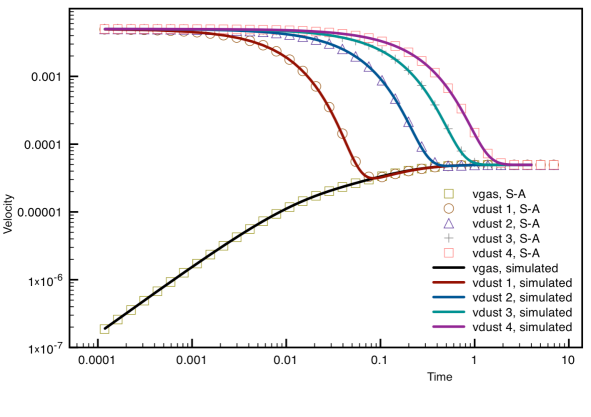
In this test problem one or multiple dust fluids start with an initial velocity difference with respect to a stationary gas fluid. Due to the drag force, the gas will be accelerated by the dust, and all dust species will decelerate at a rate imposed by the properties of the fluid. Laibe and Price (2011) presented analytical solutions for multiple drag laws in the presence of a single dust fluid and compared this with simulations in Laibe and Price (2012). To demonstrate the validity of our implementation, we compare a simulation with four dust species using the physical drag force described in equation (40) with the semi-analytical solution of the problem. In the case of one dust species, the analytical solution of the change in velocities of the dust and gas fluid are given in Laibe and Price (2012). We expand this approach to give a solution for an arbitrary number of dust fluids with the drag force in equation (40), which leads to a set of coupled nonlinear ordinary differential equations for the time dependent functions , namely
| (42) |
with the number of dust fluids. Note that the terms are functions of , as can be seen for the Epstein-Stokes drag in equation (40). We can solve this set of differential equations using a Python script to find a semi-analytical solution. For the case of one dust fluid, we recover the analytical solution mentioned earlier.
We use a setup in 1D, using a uniform grid with 40 cells and periodic boundary conditions. Note however that the setup itself is resolution independent. We set uniform gas and dust densities, with g cm-3, and a total dust mass which is a 100 times lower (). Velocities are set to and cm s-1 for all dust species. The gas temperature is set to , giving a sticking coefficient in equation (41). As numerical scheme we use the TVDLF solver (Tóth and Odstrčil, 1996) with a two-step time integration and a ‘Woodward’ type slope limiter (Colella and Woodward, 1984). We use a CFL number of 0.2. The result of the simulation with four dust species, compared with the semi-analytical solution, is given in figure 1. We see that a perfect fit between the simulation and the semi-analytical solution is obtained. The simulation demonstrates how the four dust fluids start with a velocity difference relative to the gas fluid. Due to the interaction with the gas, the dust fluids decelerate. Species 1 represents the smallest particles, and can be seen to decelerate faster than the other dust fluids. Larger dust grains have a higher inertia and take longer before they come to an equilibrium velocity with the gas.
3.3.2 Dustywave
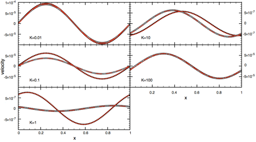
The dustywave problem, described in detail in Laibe and Price (2011), describes the propagation of a linear sound wave in a uniform and stationary medium with one or more dust fluids embedded. The coupling of the waves in the gas and dust fluids as well as the dampening of the waves are strongly dependent on the dust-to-gas ratio and the strength of the drag force. An analytic solution for a mixture with one dust fluid is known (Laibe and Price, 2011), and is used here to demonstrate the accuracy of our simulations.
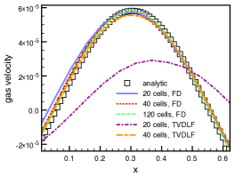
Following Laibe and Price (2011), we use , , and use one dust species. Likewise, we use the isothermal equation of state and a speed of sound . A sine-shaped perturbation in velocity and in both gas and dust densities is added, in all cases the amplitude of the perturbation is and the wavelength is the same as the size of the domain. We simulate this setup in a 1D domain between and with several resolutions. For testing purpose and comparison, we use now a simplified drag force , with a constant. We use the FD solver together with the fifth order MP5 limiter and the SSPRK(5,4) time integration using a CFL number of 0.5. In figure 2 the simulation results at time for simulations with weak () up to strong drag () are compared with the analytical solution. All simulations have the same resolution (, i.e. 120 cells with no AMR). For intermediate coupling ( between 0.1 and 10), the solutions for the dust and gas velocity can be seen to be out of phase. This phase difference causes strong damping in the setups with and . All cases are in good agreement with the analytic results and errors are typically below . Importantly, in other approaches such as the SPH method in Laibe and Price (2012) overdamping of the velocity is seen for due to the high drag force when the spatial resolution is low, leading them to propose a resolution criterion , with the stopping time , which would in this test mean about 200 cells. However, figure 3 demonstrates that by using high-order schemes we obtain results without overdamping with as little as 20 cells. In contrast, if we use a TVDLF scheme with ‘Woodward’ type limiter (Colella and Woodward, 1984) and a two-step time advance with a CFL number of 0.2, figure 3 shows that stronger dampening is observed for the case with 40 cells ( at peak value, compared to only for 40 cells with the high-order schemes). Lowering the resolution to 20 cells, a strongly dampened and shifted solution is found.
3.3.3 Sedov blast wave with dust species
The Sedov blast wave problem is a classical problem in which a high energy perturbation is introduced in a static background, causing a shockwave to propagate through the external medium. It is often used to test codes, see for example Tasker et al. (2008) who compare the ability of several fluid and SPH codes to simulate the Sedov blast wave problem. A version with one dust fluid is discussed in Laibe and Price (2012). In the gas-only case, an analytical solution for the location of the blast wave is known.
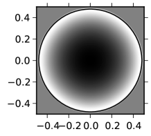
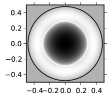
Our ambient medium has uniform gas density g cm-3 and a dust-to-gas ratio using four dust species. The pressure is set to dyn cm-2, except in the middle of the domain where we introduce a high pressure ( dyn cm-2) in a spherical region with a radius of 0.01 parsec. The gas fluid has an adiabatic index of . The simulations are performed in 3D with Cartesian coordinates, in a cubical domain with sides of one parsec. The boundaries have open outflow conditions. We use three levels of AMR, resulting in an effective resolution of 4003. With this resolution the middle region is covered in 280 cells, resulting in a total central energy erg. We use the TVDLF solver with a three-step time integration and a ‘Woodward’ type slope limiter. We use a CFL number of 0.4. Figure 4 shows a 2D output of the gas density in the 3D domain integrated along the line of sight using the collapse feature of MPI-AMRVAC, as described in the appendix B. The position of the shock front at time has been calculated analytically in Sedov (1959) and Landau and Lifshitz (1959), and is found as
| (43) |
with the energy in the central region, for an ideal gas with (Tasker et al., 2008) and ambient density . We simulate up to s (10 years), at which time equation (43) predicts a distance of 0.483 pc. Figure 4 demonstrates that the same radius is obtained in our simulations with an addition of dust with .
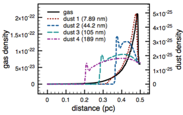
In figure 5, a 1D cut is made, showing clearly the distance the gas and dust fluids have propagated. As the gas shock propagates through the ambient medium, dust is accelerated as well. Small dust particles are more strongly coupled to the gas, resulting in a density peak close to the location of the shock. The density of dust species one is closely coupled to that of the gas. We see in figure 4 how the dust separates in regions dependent on the size of the particles. Figure 5 shows how dust species two, three, and four have two peaks. The one closest to the shock is due to the steady acceleration of ambient dust particles by the gas shock. The second peak is the result of the initially high velocity of the gas, which accelerates dust to a velocity which depends on the particle size, as large dust particles take longer to accelerate. As this high velocity dust moves outward, it sweeps up the dust in front of it, causing the second peak. Dust species one only has one peak, as the initially accelerated dust moves along with the gas.
3.4. Cloud shock in gas-dust settings
Our final gas-dust application models the interaction of a high density structure with a shock wave. This test is clearly of relevance in the interstellar medium (ISM), where dusty clouds are often seen to interact with supernova shocks. In the interstellar environment the stability of high density structures is of importance in estimating the rate of stellar formation. Numerically, the cloud is often modeled as a spherical high density structure embedded in a lower density ambient medium, with a planar shock wave propagating through the domain (Patnaude and Fesen, 2005; Nakamura et al., 2006; Agertz et al., 2007). The interaction between the shock wave and the cloud can cause several instabilities, which may lead to the disruption of the cloud. Here, we demonstrate the ability to add dust to the setup in both the cloud region and the ambient medium.
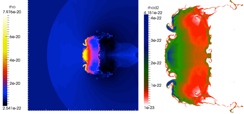
The cloud shock test is simulated in a 2D Cartesian domain with size (3.34 pc)2. We use six levels of AMR to obtain an effective resolution of 51205120. The ambient medium and the cloud, which has a radius of 0.57 pc, are initially stationary. In the surrounding medium we have g cm-3 and in the cloud . The pressure is set using
| (44) |
with the Boltzmann constant, the hydrogen mass and the molecular weight of the ISM at K. On the left side of the simulation we introduce a shocked region with values and calculated from the Rankine-Hugoniot conditions, viz.
| (45) | |||||
| (46) | |||||
| (47) | |||||
| (48) | |||||
| (49) | |||||
| (50) |
with Mach number and . This results in the initial values , and with representing the speed of sound in the ambient medium on the right hand side. In this simulation we use two dust species with everywhere. We use the TVDLF solver (CFL number 0.1) with a ‘Koren’ type limiter (Koren, 1993) and a three-step time integrator. In this simulation the gas can be seen to follow the typical evolution expected from the interaction of a supersonic shock, as shown on the left side of figure 6. While the dust also interacts with the shock, in this case the chosen size and density values of the cloud imply that the two dust species used in the simulation (like before, having sizes between 5 nm and 250 nm) are strongly coupled to the dynamics of the initial gas in the cloud. While the dust itself is not sensitive for the development of the Richtmyer-Meshkov or Rayleigh-Taylor instabilities, clear imprints in the dust distribution are visible. A more detailed discussion of the effect of dust on the latter instability can be found in Hendrix and Keppens (2014).
4. Modules for solar applications
For solar physics applications, the MHD module of MPI-AMRVAC offers a fairly diverse choice of options to model typically magnetically dominated dynamics. By selecting the appropriate combination of settings for pre-compilation of this physics module, this choice encompasses zero-beta simulations, isothermal MHD at finite plasma beta, MHD in ideal to visco-resistive prescriptions, extensions to Hall-MHD, and many sources and sinks that play a role in the radiative plasma conditions of the solar corona. We first provide an overview of the implemented equations, and then demonstrate their workings on selected applications.
4.1. Magnetohydrodynamics: Maxwell’s equations and Ohms law
We will give the complete set of equations tackled by the MHD module. Due to the possiblitiy of background magnetic field splitting, the standard MHD equations take on a somewhat unusual guise which adds to the usefulness of this collection.
Starting with the homogeneous Maxwell’s equations
| (52) |
the MPI-AMRVAC MHD module allows the user to split off a time-invariant potential magnetic field, i.e. writing
| (53) |
Note that then and . The most general form for the electric field implemented in the code writes the generalized Ohm’s law as
| (54) |
The first RHS term is applicable for an ideal MHD scenario, in a perfectly conducting plasma. The last term is related to resistivity, with resistivity parameter . The Hall (middle) term introduces a first ion-electron distinction within a single fluid plasma description, where is related to the ions, quasi-neutrality dictates for ion number density and charge number , so we can write
| (55) |
where the Hall parameter (dimensionalized555When the dimensions are fixed through a reference density , a reference length and a reference field strength , we measure speeds with respect to the Alfvén speed and the unit of mass is , while the time unit is . Then, the dimensionalized parameters are actually , also referred to as the dimensionless Lundquist number, while . The latter uses the reference ion gyrofrequency .) appears next to the resistivity parameter . Ideal MHD then sets , resistive MHD has at finite resistivity, and Hall MHD has finite values for both parameters.
If we insert the electric field expression (55) into the Maxwell equations (52), and employ the splitting (53), we obtain as evolution equation for the magnetic field the following
| (56) |
This directly corresponds to the numerical implementation where the terms in square brackets are treated as fluxes while the resistivity is added as a source.
The resistive source can be added in two ways. We note the equivalence of
| (57) |
and the RHS lends itself to implementing an alternative evaluation using a compact stencil for the discretized Laplacian ().
Note that since the Hall-current directly enters in the flux, additional layers (and ghost zones) are required in the Hall MHD case. For finite volume, this implies an additional reconstructed layer, while in a finite difference setting, only the overall stencil is increased. For the computation of the currents we have implemented second and fourth order central differencing.
4.2. treatments
As thoroughly investigated by Tóth (2000), controling solenoidality for magnetic fields in shock-capturing schemes can follow many approaches. Especially those handled by adding source terms (Powell et al., 1999) or additional equations that advect and diffuse monopoles (Dedner et al., 2002) are easily carried over to AMR settings, and several source terms strategies were already intercompared in Keppens et al. (2003). In order to control the numerical monopole errors introduced when large gradients arise and nonlinearities in the limited reconstructions exist, equation (56) is replaced by one of the following options.
An error-related source term (Powell et al., 1999; Janhunen, 2000) is added when writing
| (58) |
The diffusive approach (Keppens et al., 2003) writes
| (59) |
The generalized lagrangian multiplier (GLM) appears with an added extra equation in the GLM variants (Dedner et al., 2002), which we denote as being
| (60) |
The second variant writes as
| (61) |
A third variant based on Eq. (60) omits all and related source terms in the induction, energy and momentum equation. This simpler scheme is often sufficient and naturally adopts the spatial order from the reconstruction procedure.
In all GLM treatments, the source term for the variable can be handled in two ways, as originally described in Dedner et al. (2002). One can use the exact solution of to write
and prescribe either the constant factor . Another choice is to fix the ratio . It is also possible to perform the update implicitly by . In any case, we handle the source-update of the function in an operator split fashion.
4.3. Momentum equation, closure and energy equation
The momentum equation in MHD has the Lorentz force appearing, which could be added as a source term for HD on the RHS of equations (33) or (34). Employing the identity and using the splitting of the field, we actually implement
| (62) | |||||
The final term on the RHS is only present when the source term monopole approach (Powell et al., 1999) is taken. To close the system, two options exist.
-
•
We can use an isothermal (e.g. used in the finite beta, stratified solar flux rope formation simulations by Xia et al. (2014)) or isentropic closure as . Zero beta conditions prevail when .
-
•
In the second option, we additionally solve an evolution equation for the partial energy (-density)
(63) This energy is the total energy when no splitting of the field is adopted. When splitting is adopted, the total energy is recovered as . The governing equation for is obtained by combining the internal energy equation (38) (which has an extra RHS contribution from Ohmic heating), the velocity evolution equation ( equation (33) with the Lorentz force added), and the induction equation for the split off field (in fact equation (56)).
Collecting all together, this yields
| (64) | |||||
The heat conduction now contains only field-aligned heat transport since we adopt (note the total field here). The terms related to monopole control may not all be present (GLM introduces , and source-based may use , depending on the importance of strict energy conservation). A compact stencil evaluation of the resistive source term (activated with compactres=T) may employ .
4.4. Conservative Hall MHD
As the Hall MHD module is a new addition to the code, we list here the specifics of its implementation. Activation of Hall MHD adds terms proportional to to the fluxes in the induction equation (56) and in the partial energy equation (64). A straight-forward implementation can be provided for conservative finite differences and finite volumes using an HLL-type Riemann solver or a TVDLF-type scheme where no Riemann problem is solved (see e.g. the review of Yee, 1989). Recent implementations of Hall MHD were also provided by Lesur et al. (2014) for the PLUTO code, by Bai (2012) for ATHENA and Tóth et al. (2008) for BATSRUS. The crucial ingredient in Hall MHD is that the current enters in the fluxes resulting in a non-hyperbolic set of PDEs.
-
•
For finite volume discretisation, the strategy is to obtain from the interface values of the reconstructed magnetic field. In cartesian coordinates, second and fourth order finite differencing yields for the -component of the current vector
(65) (66) where the notation denotes the grid interface in the -direction while the remaining directions remain with centered indices everywhere. The interface magnetic field in these equations is obtained either with left biased or with right biased stencil yielding the currents and respectively. This interface current is then used along with the corresponding reconstructed variables to either compute fluxes according to Rusanov (1961) and update the state vector directly (yielding the TVDLF scheme) or to use with an HLL-type Riemann solver (see below).
- •
For upwinding () and the explicit time-step criterion (), the new local fastest wave speeds given by
| (67) |
are used, where we take the maximum of the ordinary MHD fast velocity and the fast-type whistler wave in field direction with wave number . The latter signifies the largest wave number allowed in the grid, where the maximum is taken over all grid-directions . We have found that the value of can often be reduced by a factor of two without seriously affecting the stability.
A HLL-type Riemann solver then follows naturally, giving the flux
| (71) |
where again superscript L,R signifies the quantity on the interface derived from reconstructed variables with left- and right-biased stencil respectively. The minimal and maximal signal speeds are then obtained according to Davis (1988) from
| (72) |
This parallels the implementation given by Lesur et al. (2014). The TVDLF scheme follows with the setting
| (73) |
Finally, numerical stability requires a time step satisfying
| (74) |
which becomes for small . As with explicit integration of diffusive terms, the time step will thus eventually become prohibitively small. Using high order finite differencing to obtain high accuracy at moderate resolution can yield some mitigation to this problem.
4.5. Selected tests and applications
In what follows, we present a fair variety of tests and applications that make use of the novel additions to the MHD physics module specifically, combined with the algorithmic improvements that are generic to all physics modules. We cover 3D ideal MHD wave tests for demonstrating observed accuracies, the possibilities for using high order FD schemes on shock tube problems, and several novel tests for Hall MHD scenarios. Solar physics applications illustrate the possibilities for splitting of potential magnetic fields, and a typical 3D magnetoconvection study.
4.5.1 3D Circular Alfvén wave
As the first standard test case to check the convergence of the conservative finite-difference scheme, we consider a circularly polarised Alfvén wave. This incompressible wave is also a solution to the non-linear ideal MHD equations. The setup is identical to Mignone et al. (2010) and the wave in -direction reads:
| (75) |
with the phase and phase velocity given by the Alfvén speed . The negative (positive) sign in the magnetic field components indicates a wave propagating in positive (negative) -direction. We set for the amplitude and use uniform background parameters and . The wave-vector is given by and and we rotate the vectors given by Eq. (75) accordingly. The 3D domain is given by , and and we run the setup (without AMR) over one period .
The resulting convergence of the GLM-MHD state vector is shown in and norms in the left panel of figure 7 for the third and fifth order reconstructions.
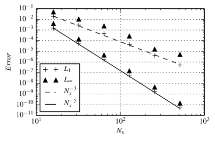
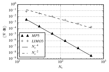
We combine LIM03 reconstruction (Čada and Torrilhon, 2009) with the third order TVD time integration (RK3) by Gottlieb and Shu (1998). As expected, third order convergence is achieved in both norms. Despite the formal fourth order of the SSPRK(5,4) by Spiteri and Ruuth (2002), we obtain fifth order convergence when using MP5 reconstruction. In the right panel of figure 7, we show the divergence error of the magnetic field for both realisations. In both cases, we calculate the divergence using fourth order central differences. As expected, the divergence of the magnetic field decreases with order given by the order of the spatial reconstruction minus one which demonstrates the effectiveness of the GLM approach.
4.5.2 Shocks, discontinuities and high order FD schemes
To investigate how the naive FD scheme handles discontinuous flows, we run a classical 1D MHD shock tube test from Brio and Wu (1988). This standard test was also adopted by Ryu and Jones (1995); Jiang and Wu (1999); Mignone et al. (2010). In terms of the primitive variables, the initial Riemann problem reads
| (78) |
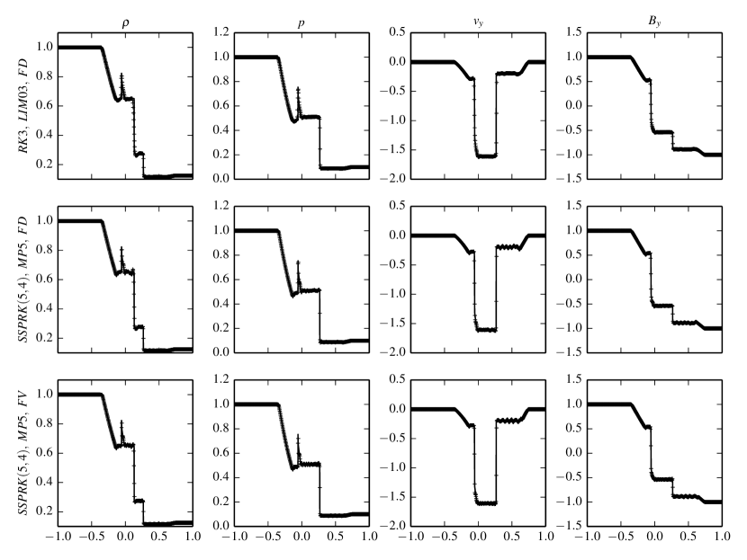
and we adopt a ratio of specific heats of . The uniform grid is composed of cells with . In addition, a reference solution is obtained with a 2nd order TVD scheme at a ridiculously high resolution of cells. Figure 8 collects our results with the schemes: RK3-LIM03-FD, SSPRK(5,4)-MP5-FD, SSPRK(5,4)-MP5-FV. Due to their conservative nature, all schemes capture the general shock structure well. At the contact discontinuity we obtain over(under)-shooting in the density by for RK3-LIM03-FD, for SSPRK(5,4)-MP5-FD and for SSPRK(5,4)-MP5-FV. The level of oscillations in the third order scheme is encouraging despite the omission of characteristic reconstruction. With fifth order reconstruction, the oscillations could be considered prohibitive for some applications. Note that the oscillations visible for example in the profiles of are not a trademark of FD discretisation alone as our FV solution shows a similar behaviour.
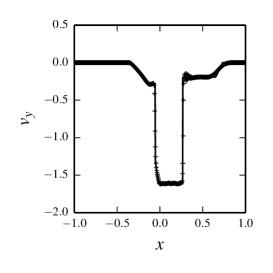
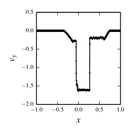
The advantages of the simple FD scheme become apparent when one considers the speedup. Relative to RK3-LIM03-FD the execution times become for SSPRK(5,4)-MP5-FD : SSPRK(5,4)-MP5-FV. Thus the FD scheme is faster than its (HLLC-based) FV counterpart by a factor of as no Riemann problems are solved. Exploiting the SSP nature of the Runge-Kutta schemes, we ran the shock tube also at the maximal CFL yielding SSP. The results are shown in figure 9. Here the third order scheme shows an excessive overshoot while the level of oscillations in the fifth order scheme is comparable to the case with Courant number 0.4. It is important to note that the amount of oscillations gets dampened in time as illustrated in the right-hand panel of figure 9.
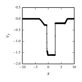
As mentioned in section 2.2, the FD scheme tends to diffuse tangential discontinuities. To check the severity of this limitation, we run the following hydrodynamic test: We initialise a contact discontinuity with large density jump between and , uniform pressure and ratio of specific heats . Thus the sound speed becomes and . The decay of the stationary contact discontinuity is investigated in spherical coordinates where we align the density profile with the -coordinate. Here, we use a 1D domain with with 64 grid points and density jump located at , the Courant number is set to 0.6. For the moving contact, we adopt slab geometry and periodic boundary conditions and choose an advection velocity of . In this case, the domain spans discretised with 128 grid points. The density jumps at and . In figure 10, we compare the states obtained with the HLLC, HLL and FD scheme at (corresponding to several hundred sound crossing times). In all these cases, MP5 reconstruction and SSPRK(5,4) time stepping is employed.
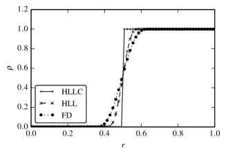
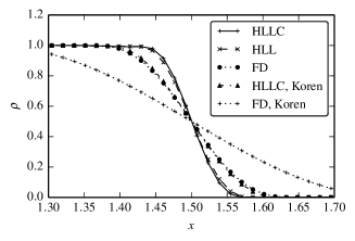
As expected, HLLC preserves the stationary contact exactly, while HLL and FD are subject to numerical diffusion. The Lax-Friedrich split FD scheme is more diffusive than the HLL solver. For the advected discontinuity, HLLC looses its capacity to capture the contact exactly and we find that the results for HLLC and HLL almost coincide. Again, the FD scheme is the most diffusive of the three. In this setup, the level of diffusion for the FD scheme is comparable to a second-order HLLC scheme with Koren reconstruction. The latter is indicated as “HLLC, Koren” in the right panel of figure 10. When run without high order reconstruction, dissipation in the FD scheme is clearly excessive (see line labeled “FD, Koren”).
4.5.3 Circular Alfvén-Whistler wave
In analogy to the MHD case, we can derive the equation for the circularly polarised Alfvén-Whistler wave. One can easily show that the wave is also a solution of the non-linear Hall-MHD system. The non-linear circularly polarised Alfven-Whistler wave in -direction reads:
| (91) |
with
| (92) |
and the phase and wave number . is the wave amplitude, not necessarily small. The phase velocity follows from the Hall MHD dispersion relation for propagation along the magnetic field
| (93) |
as
| (94) |
which reduces to the Alfvén speed in the limit . In this limit, the solution is just the circularly polarised Alfvén wave of ideal MHD. The parameter corresponds to the Alfvén gyro radius as with the ion gyro frequency . Note that the code-parameter is connected to via .
As the electron velocity depends on the current in the Hall approximation, the Alfvén-Whistler wave test is an inherently three-dimensional problem. It can be used to test the realisation of the dispersion relation (93) as well as the convergence order of the code in 3D.
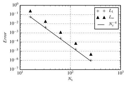
The setup of the test case is as follows: We choose , with and the state Eq. (91) is rotated accordingly. The Alfvén ion-gyro-radius is set to and we choose the plasma background parameters to satisfy . The wave amplitude is . A 3D cartesian box with edge length is simulated with the finite differencing algorithm for one period
| (95) |
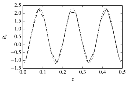
using increasing resolution starting at cells. The result of this test is presented in figure 11. It shows fourth order convergence as expected based on the use of fourth order central differencing of the current. In addition, the dispersion relation Eq. (93) is realised by our code with increasing accuracy as the resolution is increased. The right-hand panel of figure 11 demonstrates the low numerical diffusion obtained with the high-order scheme: already at a resolution of , by eye, it is hard to distinguish the profile of the propagated wave (gray) from the analytical expectation (black).
4.5.4 Group diagram in Hall-MHD
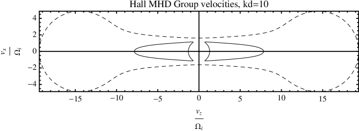
A further test for the Hall-MHD module is the Friedrich diagram of the group velocity as known from the pure MHD case. This classical example of MHD wave propagation can be used to study the transition from the ideal to the Hall MHD regime and provides a qualitative comparison for our Hall-MHD module. The Hall-MHD group diagram was first shown in Hameiri et al. (2005) and differs greatly from the ideal MHD case. In particular, the Alfvén-type ray surfaces – only points in the ideal MHD case – change dramatically and develop an extended front as illustrated in the lower panel of figure 12. Since the Hall-MHD system is not purely hyperbolic, the group diagram yields only an approximate “envelope” drawn by the fastest waves present.
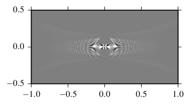
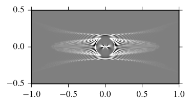
Our numerical realization of the group diagram initialises a (small) point-perturbation of a homogeneous medium threaded by a constant magnetic field in -direction (see also Keppens et al. (2012)). The grid is adaptively refined to the sixth level, starting at a base resolution of cells within a domain . We again use the solver combination SSPRK(5,4)-MP5-FD yielding formally fourth order accuracy in space and time. Information on the perturbed state is transported by slow, Alfvén and fast wave packages that form the group diagram. We choose the following background state: , and adopt an Alfvén ion-gyro radius of . Due to the dispersiveness of the modified Whistler waves, the group velocities in the Hall-MHD system depends on the wave-number and thus our numerical realization consists of the interference of all waves triggered by the initial perturbation. Analytic envelope functions for fast- and Alfvén-type waves can be constructed for the highest -value present in the system, which in our explicit implementation depends on the numerical resolution. In figure 12, we show realizations of the Friedrich diagram test in snapshots of out-of-plane velocity and pressure. An effective resolution of cells was used for this test, resulting in maximal wavenumbers . In contrast to the MHD case, the highly anisotropic (fast-type) Whistler waves propagate most rapidly in the direction of the magnetic field. Interference between the individual waves scrambles the signal, however we can clearly make out two distinct types of waves. These are the fast-type and Alfvén-type waves as illustrated in the bottom panel of figure 12.
4.5.5 Hall MHD reconnection
Magnetic reconnection plays a key role in plasma physics and many studies ranging from stationary resistive MHD (Parker, 1957) over time-dependent MHD simulations up to full PIC (particle in cell) simulations have been performed to date (see the discussion in Keppens et al., 2013). To test our code at a challenging problem, we employ the so-called double-GEM setup adopted from the well-known Geospace Environment Modelling (GEM) challenge. Ideal Hall MHD reconnection was first employed to the GEM setup by Ma and Bhattacharjee (2001). The main difference in our setup to the classical GEM challenge is that the domain contains two alternating current sheets which allows to employ doubly periodic boundary conditions, facilitating inter comparison between codes and checks on exact conservation properties (Keppens et al., 2013).
For completeness, the setup is described below. The domain is a 2D cartesian square with dimensions with and the current sheets are located at and . An ideal gas equation of state is adopted with ratio of specific heats . We employ the magnetic field
| (96) |
with perturbations
where the magnitude of the perturbation is set to , a factor of 10 lower than the background field amplitude .
The density profile is taken as
| (97) |
and an MHD equilibrium configuration is obtained via the pressure profile
| (98) |
Thus far, the setup differs from Keppens et al. (2013) only in the higher atmospheric density (outside the current sheets) with a value of in equation (98), compared to in the original study. As the Hall MHD evolution involves low plasma beta regions, the latter proved necessary to assure numerical stability. This choice of parameters results in plasma , atmospheric Alfvén velocity and sound speed . We choose an Alfvén ion-gyro radius of with the setting . Resistivity is chosen as and we adopt a dynamic viscosity of . In these runs, we employ a base-resolution of cells and add adaptive refinement based on variations in density (following the prescription of Lohner, 1987) to a total of three (low resolution case) and four levels (high resolution case).
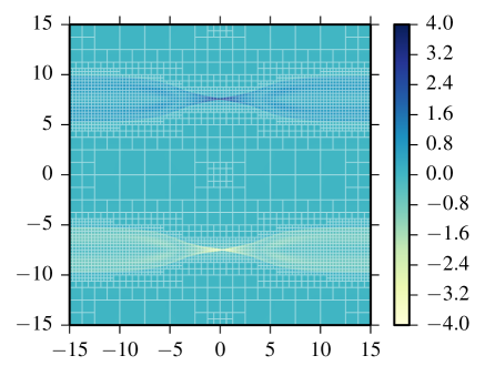
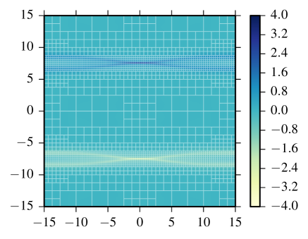
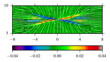
The evolution of the high resolution run is portrayed in figure 13. We observe the rapid development into an X-point, through which reconnection of magnetic field proceeds. By contrast, the visco-resistive MHD case shown in the right panel of figure 13 develops a near stationary current sheet with well defined aspect ratio.
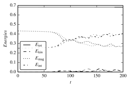
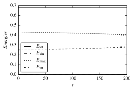
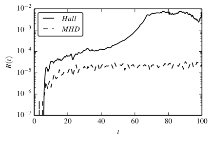
The energetics of the reconnection process is shown in figure 14. In the Hall MHD case, the initial magnetically dominated equilibrium reaches equipartition between internal and magnetic energy at . This is also where the dissipation rate peaks. Afterwards, the thermal energy increases more gradually and we observe fluctuations in the energetics that stem from compressive waves permeating the system. On the other hand, in the resistive MHD case the dynamics is dominated by Ohmic heating and the dissipation rate is nearly constant up to . Conservation of total energy is granted with a relative error of in the Hall case and with in the purely resistive case. This small energy error stems from the fact that resistive terms are currently not added in a conservative fashion. As noted previously (e.g. Shay et al., 2001; Birn and Hesse, 2001), inclusion of the Hall term is vital to obtain reconnection rates comparable to full kinetic descriptions. Indeed, the reconnection rate of the in-plane flux shown (see e.g. Fitzpatrick (2004) for a definition of this rate of reconnected flux) in figure 15 (right panel) increases over the resistive MHD case by over a factor of 100.
In Hall-MHD, electrons and ions decouple on the scale of the ion-gyroradius. Ideal Hall-MHD retains the frozen-in condition of ordinary MHD, however field-lines are advected only with the electron flow. The stream-lines in our reconnection setup are drawn in the vicinity of the X-point in the left panel of figure 15. It shows the decoupling on the scale of the Alfvén ion-gyroradius with momentary electron streamlines (black) and ion streamlines (white) on a background of the parallel electric field component . Upon entering the reconnection region, electron- and ion-flows are well aligned. In the regions of strong at the “wings” of the X-point, the incoming electron-flow is deflected sharply towards the O-point. Eventually, the ion-flow is deflected as well, however owing to its higher inertia with a larger radius of curvature.
4.5.6 Options for splitting magnetic fields: Field line extrapolations
As indicated when describing the MHD equations as implemented, it is possible to split of a potential field solution , and reformulate the evolution equations in terms of the deviation from this steady background field. This is particularly useful when one wishes to follow both gradual and more violent plasma dynamics in a realistically structured, solar coronal field topology. To that end, we here demonstrate the available options for generating exact potential field solutions, from actual magnetogram data. In the context of this paper, we demonstrate the availability (as additional open source modules) of frequently used models for global spherical (PFSS) models, as well as for local Cartesian box models (Green function based), and make some observations on their accuracy.
4.5.7 Global spherical PFSS model
The fundamental assumption made in the potential field source surface (PFSS) model (Altschuler and Newkirk, 1969; Schatten et al., 1969; Hoeksema, 1984; Wang and Sheeley, 1992; Schrijver and De Rosa, 2003) is that the magnetic field is potential within the coronal volume, allowing a magnetic potential to be defined such that . Since everywhere, the potential satisfies a Laplace equation, . The solution in spherical coordinates is
| (99) |
where the indicate spherical harmonic functions of degree and order and the coefficients and are determined by the imposed radial boundary conditions. By definition, , where are the associated Legendre functions and the constants are determined as
| (100) |
The photospheric boundary condition for is
| (101) |
where denotes the radial magnetic field as measured at the photosphere (quantified from a line-of-sight magnetogram). If we denote the spherical harmonic coefficients of as , such that , applying the boundary condition on for leaves us with
| (102) |
In principle, the coefficients are determined by the equation
| (103) |
with the complex conjugate of the spherical harmonic functions and the continuous spherical harmonic transform on the photospheric magnetic field. Though, instead of knowing the continuous function , we only know the values of the photospheric magnetic field at points , with and as obtained by observations. The discrete spherical harmonic transform is then given by , with
| (104) |
where the weights are obtained with the help of Legendre functions of the first kind.
The outer radial boundary condition is obtained by the “source surface” assumption. As source surface we define the sphere which is threaded by a purely radial field giving the von Neumann boundary condition . This is satisfied if is constant on this sphere and we can choose . Thus we obtain a relation between the expansion coefficients
| (105) |
Once the coefficients are determined from the magnetogram using relation (104), the coefficients for and follow from (102) using the orthogonality of the spherical harmonics. We can then determine the magnetic field from the equation , or written out per component we get:
| (106) | |||||
| (107) | |||||
| (108) |
where the factor is defined as . Note that the field components are real, while all are actually complex numbers.
4.5.8 PFSS extrapolation for Carrington Rotation
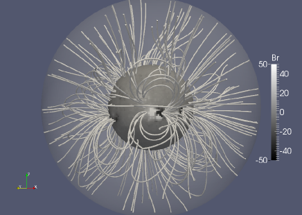
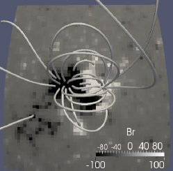
Synoptic magnetograms with resolution can be used as input to estimate the solar coronal magnetic field. We can routinely use inputs from GONG observations666The Global Oscillation Network Group (GONG) is a community-based program to conduct a detailed study of solar internal structure and dynamics using helioseismology, see http://gong.nso.edu/. at resolution and from MDI at resolution . MDI is an instrument onboard SOHO, the Solar and Heliospheric Observatory777See http://sohowww.nascom.nasa.gov/, a project of international collaboration between ESA and NASA to study the Sun from its deep core to the outer corona and the solar wind. We make use of these magnetograms after performing a magnetogram remeshing technique using the Chebyshev collocation method (e.g. Carpenter and Gottlieb, 1995). The latter interpolates the original grid where grid points are spaced equally in onto a uniform -grid. Here we present a study for the solar Carrington rotation number in 2005, using observations from the space telescope instrument MDI. We pay particular attention to two active regions within , one located at the North hemisphere and one at the South hemisphere . These two dominant active regions on each hemisphere will be used to (1) compare the global potential field source surface spherical extrapolation approach and a local potential field Cartesian one, and (2) to understand the influence of raising the number of spherical harmonics. For the latter, we will take active region as the photospheric region on which we examine the radial magnetic field variation over a line crossing the active region’s opposite polarities, as influenced by the number of spherical harmonics taken. In Figure 16, we first present an impression of the global magnetic field topology obtained from the full MDI magnetogram, used to generate a PFSS model up to using and exploiting a 3-level block-AMR grid with effective resolution .
|
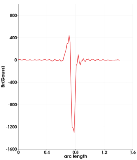
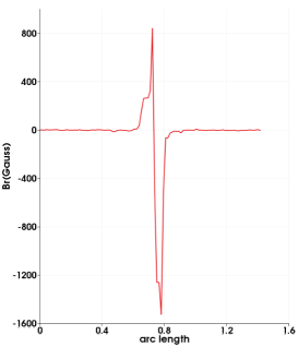
In order to investigate the effect of the number of spherical harmonics that we include in our computations on the accuracy of our results, we construct several PFSS models and compare them to a reference case. For this comparison purpose, all these models exploit a fixed uniform resolution , but we vary , where is the maximum degree of the spherical harmonic functions used in each case for the magnetic field calculation. The case with determines our reference case, since it is the maximum degree we can use for MDI magnetograms according to alias-free conditions as mentioned by Suda and Takami (2002): . In order to compare the different runs, we examine the radial component of the magnetic field on the photosphere as it varies along a line that crosses active region , as demonstrated in figure 17. As the number of spherical harmonics increases, the magnetic field maximal amplitude grows and gradually approaches the reference case variation. At the same time, the intensity of the ringing effect (Tóth et al., 2011) affecting the magnetic field value around the active region diminishes and the curve gets smoother.

|
In order to quantify this better, we compute the errors of the magnetic field magnitude for each of the above models with respect to the reference case with maximal . In figure 18, the error calculation is demonstrated with two norms, the (lowest curves) and the norm (upper data). The solid line indicates a power law fitting curve given by and the dashed line has as an exponential fit for the norm. For the norm, the dotted line is the power law fitting curve and the dot-dashed line is the exponential fit. The two norms differ about 4 orders of magnitude for all PFSS models reported in the plot, a fact which indicates that our main errors originate from specific localized regions. This conclusion is realistic as we would expect that the main errors are introduced by the existence of regions where the magnetic field is noticed to show a sudden increase of orders of magnitude, i.e. the active regions.

4.5.9 Global versus local Cartesian extrapolation
Besides the global PFSS model using full sun synoptic maps, we also implemented a local potential field extrapolation method, useful when interested in simulating specific local active region behavior. This local Cartesian approach is using exact closed-form solutions of the force-free magnetic field boundary-value problem with the help of Green’s function method (Chiu and Hilton, 1977). When the photospheric surface corresponds to the plane, the problem still reduces to solving the Laplace equation for the magnetic potential with the photospheric boundary condition given by magnetograms. When we take as second boundary condition as , the Cartesian components of the magnetic field in Green’s function forms are given by
| (109) |
where and are the boundaries of the extracted magnetogram, and the integrals contain
| (110) | |||||
| (111) | |||||
| (112) | |||||
| (113) | |||||
| (114) |
with and the position vector squared. The above formulae allow for a constant nonzero value of , then generating a linear force-free field, while for we get the potential magnetic field solution which can be split of. This exact solution does not suffer from the need to truncate at a specific angular degree encountered when using the spherical harmonics. For the integral evaluations, a simple midpoint rule is adopted.
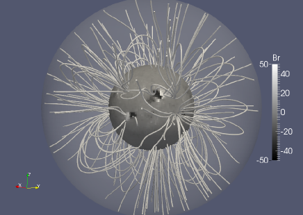
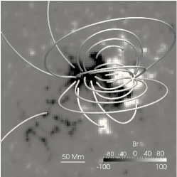
To qualitatively compare this local extrapolation method with the PFSS model in a global spherical geometry, we can do the following, all shown in figure 19. We can start from a synoptic magnetogram of a full Carrington rotation, so that the observational input is in the form of a 2D matrix of size , for MDI this is . The abovementioned Chebyshev remeshing technique is first used to transform the whole magnetogram into a uniform grid, similar to the global case. This uniform grid can be transformed into a Cartesian grid with each angular degree corresponding to a length equal to . Finally, an area of interest is extracted in Cartesian coordinates in the form of a 2D submatrix corresponding to a user selected angular part of the magnetogram. Here, we take a part containing the which counts grid points, covering a region of . We use this as a bottom magnetogram for a local extrapolation using the above method, where we use a 4-level AMR grid with effective resolution with in each direction a maximal resolving power where Mm. We also take the full MDI magnetogram as bottom boundary for a global PFSS extrapolation, this time using a uniform grid in spherical coordinates , where the radial range goes up to the source surface. This latter spherical grid ensures an effective resolving power of about on the solar suface.
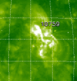
The field lines for both kinds of extrapolations are drawn in figure 19, where we show a zoomed view on the active region from the global PFSS model, and the local Cartesian result. We selected 20 specific points to start drawing the field lines. In the same figure there is also an observational EIT888Extreme ultraviolet Imaging Telescope (EIT) is an instrument on the SOHO spacecraft, sensitive to four different wavelengths 171, 195, 284, and with a minute cadence and spacial resolution of . image of the active region at 195Å, which corresponds to Fe XII and a temperature of . The two approaches show similar structure, as expected. We underline that for the local simulation, there is no source surface (the top boundary differs for the exploited Green function), a fact that explains why we have more dominant open field line topology in the right panel of figure 19. The remaining differences are due to finite curvature effects, not taken along in the Cartesian approach. The extrapolations agree only qualitatively with the observational data in the extreme ultraviolet. The (magnetically structured) plasma morphology visible at this wavelength shows similarities with the open and closed field lines of both global and local simulations, but may well deviate significantly from potential field conditions. E.g. at the center of the active region in the EIT view, a region with negative polarity differs most from the bottom magnetogram structure, as this filter shows the plasma higher inside the low corona than the photosphere itself. By inspection, the potential field extrapolation misses the implied magnetic connectivity in those regions.
|
4.5.10 Magneto-convection
As a representative, time dependent, solar application where non-ideal MHD processes are incorporated, we simulate compressible magnetoconvection in a strongly stratified layer, following Rucklidge et al. (2000). Their parametric survey focused on a prescribed polytropic atmosphere, modified with a uniform vertical magnetic field initially, and varied the field strength, the relative importance of magnetic diffusion, (isotropic) thermal conduction, and viscosity, as well as geometric parameters like the box aspect ratio. Augmented with simple boundary prescriptions fixing the top to bottom temperature contrast and fields, these authors made a systematic parameter study, identifying transitions from essentially two- to three-dimensional behavior, from kinematic to more magnetically influenced cases, from ordered to chaotic regimes. A detailed analysis of the (loss of) symmetry in the convecting endstates could benefit from group theoretical classifications using the linear eigenfunction behaviors. This allowed to obtain bifurcation diagrams, serving to classify the large variety of steady to unsteady magnetoconvection patterns. Here we will adopt two realisations, one in the steady regime and one in the unsteady chaotic parameter regime.
In a 3D Cartesian box with gravity along the negative -direction and periodic horizontal and directions, we initialize density and pressure as
| (115) | |||||
| (116) |
such that the dimensionless temperatures at top and bottom are fixed when . This dimensionalization uses the top layer temperature and density , together with the layer depth , to set dimensionless profiles and parameter values. Specifically, the atmosphere obeys hydrostatic equilibrium with dimensionless gravity parameter for gas constant . Similarly, non-ideal parameters enter for viscosity , thermal conduction and resistivity . The original study fixed the Prandtl parameter (with the ratio of specific heats where ), and then varied the initial settings through a Chandrasekhar number and a Rayleigh number . The ratio of magnetic to thermal diffusivities is dimensionally fixed by , and we will focus on cases where the related mid-layer value is set to 1.2 (the ‘astrophysically relevant situation’, as stated in Rucklidge et al. (2000)). The Chandrasekhar number was always computed from , and our dimensionalization yields the initial dimensionless magnetic field strength as . All parameters then become fixed by the value of the Rayleigh number , whose value at mid-layer in essence determines thermal conduction through the relation
| (117) |
Note that we here employ an isotropic thermal conduction (in analogy with the original study, although MPI-AMRVAC allows for anisotropic heat conduction physics as exploited in Xia et al. (2012) and Fang et al. (2013)), together with uniform resistivity and full tensorial viscosity. We used a deterministic incompressible velocity perturbation found from
| (118) | |||||
| (119) | |||||
| (120) |
where modes with specific phases were used. Boundary conditions are double periodic sideways, while both top and bottom use symmetric conditions for density , velocity components , , with asymmetry for and , . The pressure is set in the ghost cells to with the fixed top and bottom values. A second order central differencing formula on the solenoidal constraint is used to extrapolate , while the GLM scalar in the ghost cells.
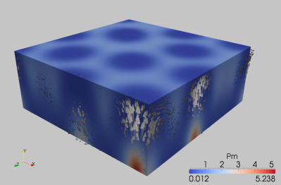
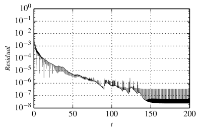
We use a multi-stage (ssprk54), finite difference scheme with MP5 reconstruction. Two cases are shown below, one (top part of Fig. 20) is at aspect ratio and , a case known to allow steady state solutions with irregular hexagons consisting of a fixed number of uprising plumes. While both an 8 and 9 plume solution were reported in Rucklidge et al. (2000), we found a 7 plume pattern which can be safely quantified as a true steady-state solution in a domain decomposition run of overal resolution . Figure 20 shows the magnetic pressure pattern in the endstate (with flow field vectors on the sidepanels), and the temporal evolution of the residual, reaching a value of after time . The slightly erratic oscillations between this value and thereafter are influenced by IO operations, which have e.g. switched conservative to primitive variables in place at selected save times.
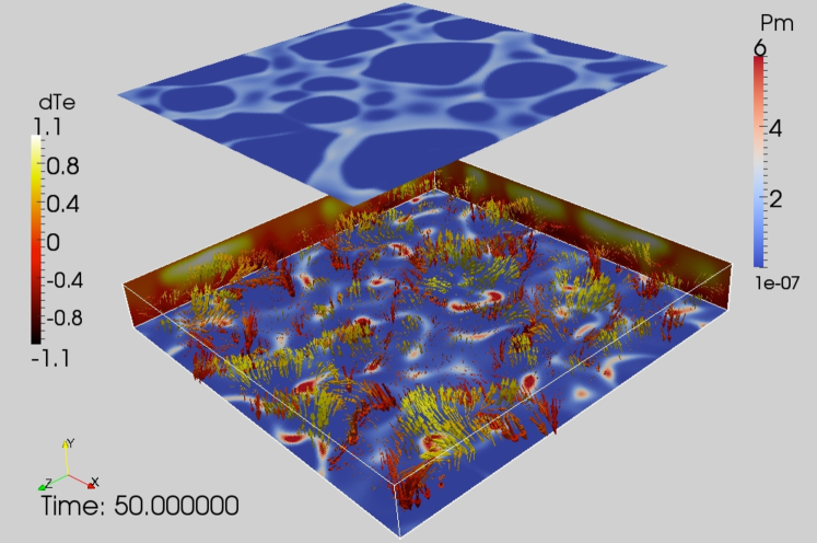
Another case is shown in the lower panel of Fig. 20, for parameters and at resolution . In this parameter regime with a very wide box, one witnesses flux separation where narrow strong field lanes surround patches that are almost field-free with vigorous convective motions. The field-free regions merge and split in a continuously evolving fashion. We show a snapshot taken at time , where the bottom and top planes are colored by magnetic pressure, the two sidepanels quantify the instantaneous temperature difference , and the velocity field is shown as arrows in the midplane, colored by this latter quantity. It shows the close relation between up versus down flows and the local temperature variations.
5. Scaling experiments
Here, we report on results of scaling experiments for MPI-AMRVAC performed on various supercomputing platforms.
5.1. Weak scaling
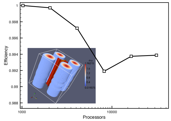
We start with a weak scaling experiment of the MPI-AMRVAC code on the BGQ Fermi computer, as quantified in Figure 21. The setup actually realizes a 3D, compressible MHD setup inspired by the discussion in Longcope-Strauss (Longcope and Strauss, 1994), where the authors argue for near-singular current sheets developing from coalescence instability. Our setup has four ‘magnetic islands’, which have purely planar () magnetic fields from and initially, in a 3D unit-sized triple periodic box. The pressure varies with to realize an equilibrium, and the temperature is uniform initially. The velocity perturbation takes a small amplitude incompressible planar , , with an extra perturbation for velocity component in the -dimension. We use resistive MHD on a uniform grid in this domain decomposition parallel scaling experiment. We use the HLLC scheme for the spatial discretisation and a third order C̆ada limiter (Čada and Torrilhon, 2009) for the time advance. To perform the weak scaling, we set up the problem with a fixed number of grid blocks per CPU (i.e. 4 blocks, each having cells, excluding ghost cells). When we increase the number of CPUs, the resolution of the simulation is increased as well, keeping the number of blocks per CPU fixed. For the smallest number of processors available on Fermi, which is 1024, the resolution is thus . At the highest number of CPUs, 31250 (almost 1 rack at Fermi), the resolution is . For each setup, we calculate 100 iterations. For all numbers of processors this takes about 1074 seconds wall clock time proving excellent weak scaling in the domain decomposition case. The obtained efficiency is plotted in the figure, and the snapshot shows a visualization of the density and current sheet structure. The four flux tubes, with initial predominant poloidal magnetic field, are susceptible to kink instability, while the central current sheet formation happens as before. An ongoing study will further investigate its fully nonlinear evolution.
5.2. Strong scaling with AMR
Strong scaling of MPI-AMRVAC using adaptive mesh refinement has been investigated on the Jade supercomputer999Centre Informatique National de l’ Enseignement Supérieur: http://www.cines.fr with the relativistic jet-formation scenario discussed in Porth (2013). For this test, we simulate one physical time-unit starting from a snapshot roughly at midpoint of the total simulation time, giving a reasonable estimate of the average workload of the simulation. The AMR-blocksize for this test is cells and two ghost cells are used on each side of the blocks. Efficiency quantification of a cell, five level production setup (case 160M) as well as small domain case with cells and four levels (case 40M) is shown in figure 22. We normalise the efficiency to the lowest processor number used, corresponding to 128 processors for case 160M and 64 processors for case 40M.101010Here, “processor” is used synonymous with “core” and thus denotes the atomic compute unit. At the lowest processor number, the simulations perform (160M) and (40M) cell-updates per second per core.
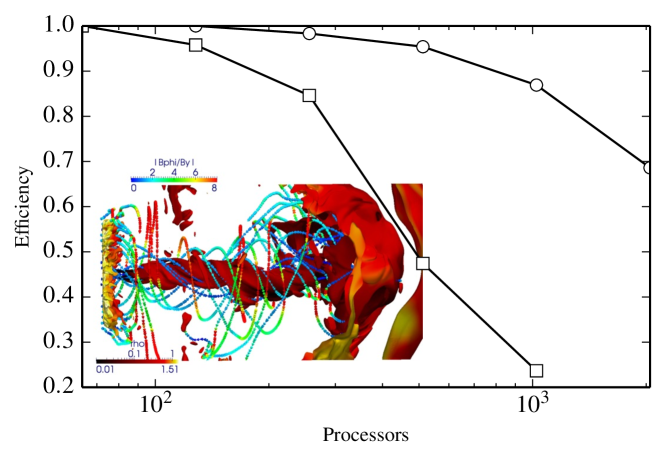
For case 40M, we quantified the AMR speedup by restarting from a corresponding snapshot where all cells were refined to the highest level.
This yields a total of blocks, to be compared to blocks on the highest level of case 40M. We would thus expect a speedup due to a more efficient space-filling by a factor of .
The observed run time comparison at 256 processors agrees roughly with this estimate and yields a speedup by a factor of when AMR is used, resulting from an AMR-overhead of approximately .
5.3. Strong scaling without AMR
A strong scaling test on a uniform grid version of the cloud shock test with one dust species (discussed in section 3.4) was performed on the SuperMUC cluster111111Leibniz-Rechenzentrum, Garching: http://www.lrz.de. We now adopt cartesian coordinates in three dimensions and use a uniform gridsize of cells (110M cells) divided in blocks (totaling 216k blocks) with two ghostcell layers on each block-face. The result of the scaling test for one “island” of SuperMuc is shown in figure 23. For this setup, we find the efficiency to actually increases with processor number up to 2048 processors. At 2048 processors we obtain the peak performance of k cell updates per processor per second. We suspect that this super-linear scaling is a result of the network configuration of the SuperMUC cluster: the tree topology allows direct communication between each individual computational node within one island. This causes the total communication bandwidth to increase when more nodes are used. As a consequence, the time spend in the routine which communicates the boundary conditions between the blocks on different nodes (see figure 23) is decreased dramatically. When more than 2048 cores are used, the efficiency drops again, as communication time is becoming predominantly latency-limited. Note that at 8192 cores, the efficiency is still as compared to 1024 cores.
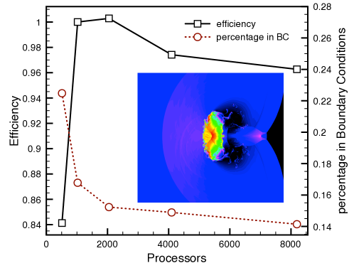
6. Summary and outlook
We provided an update on the MPI-AMRVAC development, with a focus on the latest additions to our open source repository (see http://gitorious.org/amrvac). The block-AMR, fully parallel software has many possibilities for gas dynamical and plasma physical applications, inspired by concrete astrophysical or solar physical observations. The presentation here emphasized the newest additions to the non-relativistic physics modules, although the high order FD schemes and time steppers are directly available to all physics modules, including the relativistic HD and MHD ones. In the appendices, we present details on how we produce sliced or collapsed views that fully respect the AMR structure during runtime, as well as the added benefits of being able to distinguish between active and passive grid blocks. These can be of generic interest to all complementary coding efforts on open source, grid adaptive, parallel software for astrophysical applications.
In the future, we plan to extend recent works (van Marle et al., 2011; van Marle and Keppens, 2012) on circumstellar wind interactions to cases where stellar winds interact in binary systems, extending the pure gas dynamical study by van Marle et al. (2011) to cases where radiative effects, dust creation and its redistribution over the shocked wind interaction zone are relevant. For solar applications, we intend to continue our work on prominence formation in realistic fluxrope configurations, based on the steps already taken in 2.5D MHD or in 3D isothermal MHD (Xia et al., 2012, 2014). Global as well as local solar modeling will use the potential field extrapolation possibilities in ultimately data-driven scenarios, to complement state-of-the-art simulations such as those presented by Riley et al. (2011); van der Holst et al. (2014). These can also aid ongoing efforts on global magnetospheric modeling with MPI-AMRVAC , such as those for the Jovian case as done by Chané et al. (2013).
Appendix A Slicing a Morton order AMR grid
Simulations in two and three dimensions frequently lead to large datasets that are not easily visualised. For a quick look into the -dimensional data however, it is often sufficient to examine sub-dimensional slices. MPI-AMRVAC is capable to slice any of its grids along the coordinate directions and output the dimensional data during runtime. The algorithm takes advantage of the tree based grid structure and is described below.
-
1.
Given the direction perpendicular to the resulting slice and the coordinate-value along , , for each level calculate the grid index indicated by the slice:
(A1) where is the extent of a grid block (in direction on level ) and is given by the minimal domain boundary. An exemplary 2D grid is shown in figure 24.
-
2.
For every base grid at :
-
(a)
For every child in direction other than , descend (recursively) into the child:
(A2) where the child index is defined as for the left child and for the right child.
-
i.
Upon encounter of a leaf, take the corresponding block and fill a sub-dimensional solution block given the cells closest to .
-
i.
-
(a)
-
3.
Output sub-dimensional solution block in order of their encounter.
The resulting sub-dimensional grid is again in tree-form and reflects the original adaptive mesh which can be valuable for data inspection. Due to the recursion, the new sub-dimensional space filling curve is Morton ordered. This strong correspondence between the data-structures even allows to restart an AMR run in dimensions without further modifications, implying . The presented algorithm can be applied to any dimensionality and optimally takes advantage of the grid structure since grids relevant for the slice are known a-priori (from step 1.). The outer loop thus scales as , while the complexity added by the recursive inner loop depends on the number of dimensions and levels.
Appendix B Collapsing a Morton order AMR grid
The dimensionality of the grid can also be reduced by integration along coordinate directions, thus “collapsing” the data onto a plane. This yields surface densities, etc. The following algorithm can collapse data onto any level during runtime while taking advantage of the underlying data-structure.
-
1.
Given the direction of integration and the target level of the resulting data , first sum the quantity for each block
(B1) where is the orthogonal projection of a (index-) vector along . The projection simply removes the direction in the arrays, leaving the order of the remaining directions unaffected. After this elemental collapse operation, we drop the superscript and work only in the reduced index space.
-
2.
Each processor allocates the global array for collapsed data , where the number of cells in each direction follows from the number of grid blocks in the target level and the number of cells within each block .
-
3.
Add up all collapsed blocks in the -array, using block index and level to fill the correct bins:
(B2) where is the local index in the block, the number of ghost cells and the term is added to translate from the local block cell-index to the corresponding global cell-index on level . Thus for all blocks on the processor , perform
(B3) where the term (with being the original dimensionality) results in an averaging of data on levels higher than the target level. Each process now holds a version of the array, hence the final step
-
4.
Use the MPI reduce operation to obtain
(B4)
on the head node. The final array is then written out either as comma-separated value ascii data-file or in binary .vti format.
Appendix C Dynamic grid activation
In many applications, parts of the simulation domain can well be described by stationarity or as analytic (e.g. self-similar) solutions, while other parts ask for direct numerical simulation. Examples for the “passive” regions are injected supersonic stellar winds, jets that have settled to a stationary state (starting near the injection boundary) or simply the static initial configuration that is still unaffected by the dynamical evolution. Especially for problems that involve a large separation of scales, as in the case of space weather, the computation can be significantly sped up if these passive regions are taken out of the integration loop.
We have implemented a scheme that can dynamically (de-) activate grid blocks in an AMR setting, depending on the solution itself or on temporal/spatial properties. Since the implementation acts only on the grid structure, it can directly be used with all available physics modules. In the following we describe the strategy and give an example application from recent special relativistic magneto hydrodynamics simulations (Porth et al., 2014).
-
1.
Loop over all grid blocks and flag grids to be de-activated based on a user-defined criterion.
-
2.
Loop over the candidate passive blocks and re-activate block if an active neighbour is detected.
-
3.
Create final lists of the active and passive blocks.
The second step can be repeated to increase the number of safety blocks. Note that this procedure seamlessly works across level changes. For the ensuing time-integration, only the list of active blocks is advanced. In principle, a separate loop can then also advance the passive blocks, following for example a self-similar analytic evolution or employ a completely different physics module.
With active and passive zones present, the parallel load balancing of the code needs some attention. While normally a balanced load is achieved by cutting of the space filling curve (SFC) such that the number of blocks per processor is balanced for all processors, it is clear that the introduction of passive blocks violates the identity of block and computational load. Hence we introduce different weights for active and passive blocks. This allows to better balance the true computational load and at the same time sets a limit for the permitted memory imbalance. In practise the adopted load per block is
| (C3) |
which is balanced by suitably cutting the SFC. The imbalance of load and memory considering all processors is
| (C4) |
Choosing balances the active blocks exactly but could lead to significant memory imbalance. Given the weights, the maximum permitted memory imbalance defined above is . We typically adopt which gives the best results for the problems and hardware considered so far.
In figure 25 we illustrate dynamic grid activation at the example of a relativistic pulsar wind simulation from Porth et al. (2013). Cells marked yellow in the left panel of the figure are not advanced in the time loop but hold the stationary solution of the unshocked wind. Note that in this particular application, the origin was refined up to level 20 to properly resolve the inner regions (the shock is situated on level 9). For the case that the shock is squeezed back to the pulsar, these grids can be automatically activated. In this case, the main speedup is not due to the reduced number of active grids to be advanced, but due to the larger resulting global CFL limited time step.
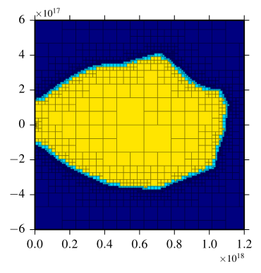
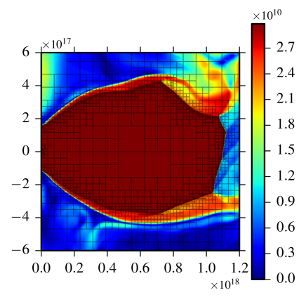
References
- Stone and Norman (1992) J. M. Stone and M. L. Norman, ApJS, 80, 791 (1992).
- Galsgaard and Nordlund (1996) K. Galsgaard and Å. Nordlund, J. Geophys. Res., 101, 13445 (1996).
- Tóth (1996) G. Tóth, Astrophysical Letters and Communications, 34, 245 (1996).
- Tóth and Odstrčil (1996) G. Tóth and D. Odstrčil, Journal of Computational Physics, 128, 82 (1996).
- Tóth (2000) G. Tóth, Journal of Computational Physics, 161, 605 (2000).
- Goedbloed et al. (2010) J. P. Goedbloed, R. Keppens, and S. Poedts, Advanced Magnetohydrodynamics, by J. P. Goedbloed , Rony Keppens , Stefaan Poedts, Cambridge, UK: Cambridge University Press, 2010 (2010).
- Balsara (2001) D. S. Balsara, Journal of Computational Physics, 174, 614 (2001), astro-ph/0112150 .
- Powell et al. (1999) K. G. Powell, P. L. Roe, T. J. Linde, T. I. Gombosi, and D. L. De Zeeuw, Journal of Computational Physics, 154, 284 (1999).
- Tóth et al. (2012) G. Tóth, B. van der Holst, I. V. Sokolov, D. L. De Zeeuw, T. I. Gombosi, F. Fang, W. B. Manchester, X. Meng, D. Najib, K. G. Powell, Q. F. Stout, A. Glocer, Y.-J. Ma, and M. Opher, Journal of Computational Physics, 231, 870 (2012).
- Tóth et al. (2005) G. Tóth, I. V. Sokolov, T. I. Gombosi, D. R. Chesney, C. R. Clauer, D. L. de Zeeuw, K. C. Hansen, K. J. Kane, W. B. Manchester, R. C. Oehmke, K. G. Powell, A. J. Ridley, I. I. Roussev, Q. F. Stout, O. Volberg, R. A. Wolf, S. Sazykin, A. Chan, B. Yu, and J. Kóta, Journal of Geophysical Research (Space Physics), 110, A12226 (2005).
- Ziegler (2008) U. Ziegler, Computer Physics Communications, 179, 227 (2008).
- Fromang et al. (2006) S. Fromang, P. Hennebelle, and R. Teyssier, A&A, 457, 371 (2006), astro-ph/0607230 .
- Cunningham et al. (2009) A. J. Cunningham, A. Frank, P. Varnière, S. Mitran, and T. W. Jones, ApJS, 182, 519 (2009), arXiv:0710.0424 .
- Mignone et al. (2007) A. Mignone, G. Bodo, S. Massaglia, T. Matsakos, O. Tesileanu, C. Zanni, and A. Ferrari, ApJS, 170, 228 (2007), astro-ph/0701854 .
- Mignone et al. (2012) A. Mignone, C. Zanni, P. Tzeferacos, B. van Straalen, P. Colella, and G. Bodo, ApJS, 198, 7 (2012), arXiv:1110.0740 [astro-ph.HE] .
- Lukin and Linton (2011) V. S. Lukin and M. G. Linton, Nonlinear Processes in Geophysics, 18, 871 (2011).
- Bryan et al. (2014) G. L. Bryan, M. L. Norman, B. W. O’Shea, T. Abel, J. H. Wise, M. J. Turk, D. R. Reynolds, D. C. Collins, P. Wang, S. W. Skillman, B. Smith, R. P. Harkness, J. Bordner, J.-h. Kim, M. Kuhlen, H. Xu, N. Goldbaum, C. Hummels, A. G. Kritsuk, E. Tasker, S. Skory, C. M. Simpson, O. Hahn, J. S. Oishi, G. C. So, F. Zhao, R. Cen, Y. Li, and The Enzo Collaboration, ApJS, 211, 19 (2014), arXiv:1307.2265 [astro-ph.IM] .
- Del Zanna et al. (2007) L. Del Zanna, O. Zanotti, N. Bucciantini, and P. Londrillo, A&A, 473, 11 (2007), arXiv:0704.3206 .
- Fryxell et al. (2000) B. Fryxell, K. Olson, P. Ricker, F. X. Timmes, M. Zingale, D. Q. Lamb, P. MacNeice, R. Rosner, J. W. Truran, and H. Tufo, ApJS, 131, 273 (2000).
- Dreher and Grauer (2006) J. Dreher and R. Grauer, Par. Comput., 31, 913 (2006), physics/0602004 .
- Freytag et al. (2012) B. Freytag, M. Steffen, H.-G. Ludwig, S. Wedemeyer-Böhm, W. Schaffenberger, and O. Steiner, Journal of Computational Physics, 231, 919 (2012), arXiv:1110.6844 [astro-ph.SR] .
- Stone et al. (2008) J. M. Stone, T. A. Gardiner, P. Teuben, J. F. Hawley, and J. B. Simon, ApJS, 178, 137 (2008), arXiv:0804.0402 .
- Arber et al. (2001) T. D. Arber, A. W. Longbottom, C. L. Gerrard, and A. M. Milne, Journal of Computational Physics, 171, 151 (2001).
- Brandenburg and Dobler (2002) A. Brandenburg and W. Dobler, Computer Physics Communications, 147, 471 (2002), astro-ph/0111569 .
- Walder and Folini (2000) R. Walder and D. Folini, in Thermal and Ionization Aspects of Flows from Hot Stars, Astronomical Society of the Pacific Conference Series, Vol. 204, edited by H. Lamers and A. Sapar (2000) p. 281.
- Gordeev et al. (2013) E. Gordeev, G. Facskó, V. Sergeev, I. Honkonen, M. Palmroth, P. Janhunen, and S. Milan, Journal of Geophysical Research (Space Physics), 118, 3138 (2013).
- Shelyag et al. (2008) S. Shelyag, V. Fedun, and R. Erdélyi, A&A, 486, 655 (2008).
- Vögler et al. (2005) A. Vögler, S. Shelyag, M. Schüssler, F. Cattaneo, T. Emonet, and T. Linde, A&A, 429, 335 (2005).
- Hayek et al. (2010) W. Hayek, M. Asplund, M. Carlsson, R. Trampedach, R. Collet, B. V. Gudiksen, V. H. Hansteen, and J. Leenaarts, A&A, 517, A49 (2010).
- Giacomazzo and Rezzolla (2007) B. Giacomazzo and L. Rezzolla, Classical and Quantum Gravity, 24, 235 (2007), gr-qc/0701109 .
- Gammie et al. (2003) C. F. Gammie, J. C. McKinney, and G. Tóth, ApJ, 589, 444 (2003), astro-ph/0301509 .
- Keppens et al. (2003) R. Keppens, M. Nool, G. Tóth, and J. P. Goedbloed, Computer Physics Communications, 153, 317 (2003), astro-ph/0403124 .
- van der Holst and Keppens (2007) B. van der Holst and R. Keppens, Journal of Computational Physics, 226, 925 (2007).
- Keppens and Porth (2014) R. Keppens and O. Porth, Journal of Computational and Applied Mathematics, 266, 87 (2014).
- Tóth (1997) G. Tóth, Journal of Computational Physics, 138, 981 (1997).
- Meliani et al. (2007) Z. Meliani, R. Keppens, F. Casse, and D. Giannios, MNRAS, 376, 1189 (2007), astro-ph/0701434 .
- van der Holst et al. (2008) B. van der Holst, R. Keppens, and Z. Meliani, Computer Physics Communications, 179, 617 (2008), arXiv:0807.0713 .
- Keppens et al. (2012) R. Keppens, Z. Meliani, A. J. van Marle, P. Delmont, A. Vlasis, and B. van der Holst, Journal of Computational Physics, 231, 718 (2012).
- Vlasis et al. (2011) A. Vlasis, H. J. van Eerten, Z. Meliani, and R. Keppens, MNRAS, 415, 279 (2011).
- Meliani and Keppens (2010) Z. Meliani and R. Keppens, A&A, 520, L3 (2010), arXiv:1009.1224 [astro-ph.HE] .
- Monceau-Baroux et al. (2014) R. Monceau-Baroux, O. Porth, Z. Meliani, and R. Keppens, A&A, 561, A30 (2014), arXiv:1311.7593 [astro-ph.HE] .
- Keppens et al. (2008) R. Keppens, Z. Meliani, B. van der Holst, and F. Casse, A&A, 486, 663 (2008), arXiv:0802.2034 .
- Walg et al. (2013) S. Walg, A. Achterberg, S. Markoff, R. Keppens, and Z. Meliani, MNRAS, 433, 1453 (2013), arXiv:1305.2157 [astro-ph.HE] .
- Porth (2013) O. Porth, MNRAS, 429, 2482 (2013), arXiv:1212.0676 [astro-ph.HE] .
- Porth et al. (2014) O. Porth, S. S. Komissarov, and R. Keppens, MNRAS, 438, 278 (2014), arXiv:1310.2531 [astro-ph.HE] .
- van Marle et al. (2011) A. J. van Marle, Z. Meliani, R. Keppens, and L. Decin, ApJ, 734, L26 (2011a), arXiv:1105.2387 [astro-ph.SR] .
- Meheut et al. (2012) H. Meheut, Z. Meliani, P. Varniere, and W. Benz, A&A, 545, A134 (2012), arXiv:1208.4947 [astro-ph.EP] .
- Hendrix and Keppens (2014) T. Hendrix and R. Keppens, A&A, 562, A114 (2014a), arXiv:1401.6774 [astro-ph.GA] .
- Beeck et al. (2012) B. Beeck, R. Collet, M. Steffen, M. Asplund, R. H. Cameron, B. Freytag, W. Hayek, H.-G. Ludwig, and M. Schüssler, A&A, 539, A121 (2012), arXiv:1201.1103 [astro-ph.SR] .
- Keppens et al. (2013) R. Keppens, O. Porth, K. Galsgaard, J. T. Frederiksen, A. L. Restante, G. Lapenta, and C. Parnell, Physics of Plasmas, 20, 092109 (2013a).
- Toro (1999) E. F. Toro, Riemann Solvers and Numerical Methods for Fluid Dynamics (Springer, 1999).
- Fedkiw et al. (1998) R. P. Fedkiw, B. Merriman, R. Donat, and S. Osher, The penultimate scheme for systems of conservation laws: finite-difference ENO with Marquina’s flux splitting, Tech. Rep. (1998).
- Rusanov (1961) V. V. Rusanov, Zh. Vychisl. Mat. Mat. Fiz., 1, 267 (1961).
- Jiang and Wu (1999) G.-S. Jiang and C.-c. Wu, Journal of Computational Physics, 150, 561 (1999).
- Mignone et al. (2010) A. Mignone, P. Tzeferacos, and G. Bodo, Journal of Computational Physics, 229, 5896 (2010), arXiv:1001.2832 [astro-ph.HE] .
- Radice and Rezzolla (2012) D. Radice and L. Rezzolla, A&A, 547, A26 (2012), arXiv:1206.6502 [astro-ph.IM] .
- van Leer (1982) B. van Leer, in Numerical Methods in Fluid Dynamics, Lecture Notes in Physics, Berlin Springer Verlag, Vol. 170, edited by E. Krause (1982) pp. 507–512.
- Liou and Steffen (1993) M.-S. Liou and C. J. Steffen, Journal of Computational Physics, 107, 23 (1993).
- Čada and Torrilhon (2009) M. Čada and M. Torrilhon, Journal of Computational Physics, 228, 4118 (2009a).
- Suresh and Huynh (1997) A. Suresh and H. T. Huynh, Journal of Computational Physics, 136, 83 (1997).
- Gottlieb and Shu (1998) S. Gottlieb and C. W. Shu, Mathematics of Computation, 67, 73 (1998).
- Spiteri and Ruuth (2002) R. J. Spiteri and S. J. Ruuth, SIAM J. Numer. Anal., 40, 469 (2002), ISSN 0036-1429.
- van Marle and Keppens (2011) A. J. van Marle and R. Keppens, Computers & Fluids, 42, 44 (2011).
- Decin (2006) L. e. a. Decin, A&A, 456, 549 (2006), astro-ph/0606299 .
- Laibe and Price (2012) G. Laibe and D. J. Price, MNRAS, 420, 2345 (2012), arXiv:1111.3090 [astro-ph.IM] .
- Sod (1978) G. A. Sod, Journal of Computational Physics, 27, 1 (1978).
- Hendrix and Keppens (2014) T. Hendrix and R. Keppens, in Proc. 8th International conference of numerical modeling of space plasma flows (ASTRONUM, Biarritz, France, July 2013), ASP Conference Series (Astronomical Society of the Pacific, San Francisco, US, 2014).
- Draine and Lee (1984) B. T. Draine and H. M. Lee, ApJ, 285, 89 (1984).
- Laibe and Price (2011) G. Laibe and D. J. Price, MNRAS, 418, 1491 (2011), arXiv:1106.1736 [astro-ph.EP] .
- Colella and Woodward (1984) P. Colella and P. R. Woodward, Journal of Computational Physics, 54, 174 (1984).
- Tasker et al. (2008) E. J. Tasker, R. Brunino, N. L. Mitchell, D. Michielsen, S. Hopton, F. R. Pearce, G. L. Bryan, and T. Theuns, MNRAS, 390, 1267 (2008), arXiv:0808.1844 .
- Sedov (1959) L. I. Sedov, Similarity and Dimensional Methods in Mechanics (New York: Academic Press, 1959).
- Landau and Lifshitz (1959) L. D. Landau and E. M. Lifshitz, Course of Theoretical Physics, Vol. Vol. 6 : Fluid Mechanics (Pergamon Press, 1959).
- Patnaude and Fesen (2005) D. J. Patnaude and R. A. Fesen, ApJ, 633, 240 (2005), astro-ph/0507330 .
- Nakamura et al. (2006) F. Nakamura, C. F. McKee, R. I. Klein, and R. T. Fisher, ApJS, 164, 477 (2006), astro-ph/0511016 .
- Agertz et al. (2007) O. Agertz, B. Moore, J. Stadel, D. Potter, F. Miniati, J. Read, L. Mayer, A. Gawryszczak, A. Kravtsov, Å. Nordlund, F. Pearce, V. Quilis, D. Rudd, V. Springel, J. Stone, E. Tasker, R. Teyssier, J. Wadsley, and R. Walder, MNRAS, 380, 963 (2007), astro-ph/0610051 .
- Koren (1993) B. Koren, A robust upwind discretization for advection, diffusion and source terms, Vol. Notes on Numerical Fluid Mechanics 45 (1993).
- Dedner et al. (2002) A. Dedner, F. Kemm, D. Kröner, C.-D. Munz, T. Schnitzer, and M. Wesenberg, Journal of Computational Physics, 175, 645 (2002).
- Janhunen (2000) P. Janhunen, Journal of Computational Physics, 160, 649 (2000).
- Xia et al. (2014) C. Xia, R. Keppens, and Y. Guo, ApJ, 780, 130 (2014), arXiv:1311.5478 [astro-ph.SR] .
- Yee (1989) H. C. Yee, A Class of High-Resolution Explicit and Implicit Shock-Capturing Methods, NASA (1989).
- Lesur et al. (2014) G. Lesur, M. W. Kunz, and S. Fromang, ArXiv e-prints (2014), arXiv:1402.4133 [astro-ph.SR] .
- Bai (2012) X.-N. Bai, Non-ideal magnetohydrodynamic effects in protoplanetary disks, Ph.D. thesis, Princeton University (2012).
- Tóth et al. (2008) G. Tóth, Y. Ma, and T. I. Gombosi, Journal of Computational Physics, 227, 6967 (2008).
- Davis (1988) S. F. Davis, 9, 445 (1988), ISSN 0196-5204.
- Brio and Wu (1988) M. Brio and C. C. Wu, Journal of Computational Physics, 75, 400 (1988).
- Ryu and Jones (1995) D. Ryu and T. W. Jones, ApJ, 442, 228 (1995), arXiv:astro-ph/9404074 .
- Hameiri et al. (2005) E. Hameiri, A. Ishizawa, and A. Ishida, Physics of Plasmas, 12, 072109 (2005).
- Keppens et al. (2012) R. Keppens, Z. Meliani, A. van Marle, P. Delmont, A. Vlasis, and B. van der Holst, Journal of Computational Physics, 231, 718 (2012), ISSN 0021-9991.
- Parker (1957) E. N. Parker, J. Geophys. Res., 62, 509 (1957).
- Keppens et al. (2013) R. Keppens, O. Porth, K. Galsgaard, J. T. Frederiksen, A. L. Restante, G. Lapenta, and C. Parnell, Physics of Plasmas, 20, 092109 (2013b).
- Ma and Bhattacharjee (2001) Z. W. Ma and A. Bhattacharjee, J. Geophys. Res., 106, 3773 (2001).
- Lohner (1987) R. Lohner, Computer Methods in Applied Mechanics and Engineering, 61, 323 (1987).
- Shay et al. (2001) M. A. Shay, J. F. Drake, B. N. Rogers, and R. E. Denton, J. Geophys. Res., 106, 3759 (2001).
- Birn and Hesse (2001) J. Birn and M. Hesse, J. Geophys. Res., 106, 3737 (2001).
- Fitzpatrick (2004) R. Fitzpatrick, Physics of Plasmas, 11, 3961 (2004).
- Altschuler and Newkirk (1969) M. D. Altschuler and G. Newkirk, Sol. Phys., 9, 131 (1969).
- Schatten et al. (1969) K. H. Schatten, J. M. Wilcox, and N. F. Ness, Sol. Phys., 6, 442 (1969).
- Hoeksema (1984) J. T. Hoeksema, Structure and evolution of the large scale solar and heliospheric magnetic fields, Ph.D. thesis, Stanford Univ., CA. (1984).
- Wang and Sheeley (1992) Y.-M. Wang and N. R. Sheeley, Jr., ApJ, 392, 310 (1992).
- Schrijver and De Rosa (2003) C. J. Schrijver and M. L. De Rosa, Sol. Phys., 212, 165 (2003).
- Carpenter and Gottlieb (1995) M. H. Carpenter and D. Gottlieb, J. Comput. Phys, 129, 74 (1995).
- Suda and Takami (2002) R. Suda and M. Takami, Mathematics of Computation, 71, 703 (2002), ISSN 0025-5718.
- Tóth et al. (2011) G. Tóth, B. van der Holst, and Z. Huang, ApJ, 732, 102 (2011), arXiv:1104.5672 [astro-ph.SR] .
- Chiu and Hilton (1977) Y. T. Chiu and H. H. Hilton, ApJ, 212, 873 (1977).
- Rucklidge et al. (2000) A. M. Rucklidge, N. O. Weiss, D. P. Brownjohn, P. C. Matthews, and M. R. E. Proctor, Journal of Fluid Mechanics, 419, 283 (2000).
- Xia et al. (2012) C. Xia, P. F. Chen, and R. Keppens, ArXiv e-prints (2012a), arXiv:1202.6185 [astro-ph.SR] .
- Fang et al. (2013) X. Fang, C. Xia, and R. Keppens, ApJ, 771, L29 (2013), arXiv:1306.4759 [astro-ph.SR] .
- Longcope and Strauss (1994) D. W. Longcope and H. R. Strauss, ApJ, 437, 851 (1994).
- Čada and Torrilhon (2009) M. Čada and M. Torrilhon, Journal of Computational Physics, 228, 4118 (2009b).
- van Marle and Keppens (2012) A. J. van Marle and R. Keppens, A&A, 547, A3 (2012), arXiv:1209.4496 [astro-ph.SR] .
- van Marle et al. (2011) A. J. van Marle, R. Keppens, and Z. Meliani, A&A, 527, A3 (2011b), arXiv:1011.1734 [astro-ph.GA] .
- Xia et al. (2012) C. Xia, P. F. Chen, and R. Keppens, ApJ, 748, L26 (2012b), arXiv:1202.6185 [astro-ph.SR] .
- Riley et al. (2011) P. Riley, R. Lionello, J. A. Linker, Z. Mikic, J. Luhmann, and J. Wijaya, Sol. Phys., 274, 361 (2011).
- van der Holst et al. (2014) B. van der Holst, I. V. Sokolov, X. Meng, M. Jin, W. B. Manchester, IV, G. Tóth, and T. I. Gombosi, ApJ, 782, 81 (2014), arXiv:1311.4093 [astro-ph.SR] .
- Chané et al. (2013) E. Chané, J. Saur, and S. Poedts, Journal of Geophysical Research (Space Physics), 118, 2157 (2013).
- Porth et al. (2013) O. Porth, S. S. Komissarov, and R. Keppens, MNRAS, 431, L48 (2013), arXiv:1212.1382 [astro-ph.HE] .