Wave-function and density functional theory studies of dihydrogen complexes

Abstract

We performed a benchmark study on a series of dihydrogen bond complexes and constructed a set of reference bond distances and interaction energies. The test set was employed to assess the performance of several wave-function correlated and density functional theory methods. We found that second-order correlation methods describe relatively well the dihydrogen complexes. However, for high accuracy inclusion of triple contributions is important. On the other hand, none of the considered density functional methods can simultaneously yield accurate bond lengths and interaction energies. However, we found that improved results can be obtained by the inclusion of non-local exchange contributions.

I Introduction

Noncovalent interactions are of fundamental importance in a vast number of chemical and physical phenomena. Thus, they are the subject of numerous computational studies sherrill13 ; hohenstein12 ; burns11 ; thanthiriwatte11 ; sherrill09 ; dubecky13 ; sedlak ; hobza13 ; melichercik13 ; riley13 ; riley13_2 ; zhao07 ; zhao06 ; johnson13 ; otero13 ; johnson13_2 ; contreras11 ; johnson10 ; grabowski13 ; noncov_book Among others, hydrogen bonds, have a prominent role in this context, due to their practical and historical importance hbond_book1 ; hbond_book2 ; kollman ; zhao12 ; grabowski11 ; li11_2 ; contreras11_2 ; johnson09 ; grabowski13_2 ; fuster11 .

A peculiar type of hydrogen bond is the dihydrogen bond in which the bonding occurs between two oppositely polarized hydrogen atoms. In the most naive physical picture it can be represented as X–H${}^{\delta^{-}}\cdots^{\delta^{+}}$H–Y, where X is an element less electronegative than H, such as Li, Be, B, Na, whereas Y is an element more electronegative than H, such as F, Cl, or CH₃. However, the nature of the bonding cannot be simply attributed only to electrostatic effects. In fact, more complicated quantum effects, such as exchange and correlation, play a prominent role in most cases and they must be properly taken into account when an accurate description of the bond is sought dihydro_book ; dihydro_rev . The complex nature of the interactions beyond dihydrogen bonding reflect the fact that dihydrogen bonds, similarly to conventional hydrogen bonds, display a strong directionality and a wide variety of strengths, ranging from few tenths of to several tens of kcal/mol, with no sharp boundary with dispersion interactions grabowski04 .

Over the last years, dihydrogen bonding has attracted great interest, because it has been found to play an important role for the structure and reactivity of both molecular complexes and solid-state systems (see for example Refs. 31; 32 and references therein). A dihydrogen bond can occur in fact between hydrogen atoms within a single molecule, or between hydrogens belonging to different molecules. Thus, it has special relevance in many different fields ranging from organic chemistry to crystal engineering and catalysis. Moreover, a dihydrogen bond can be viewed as a precursor to dehydrogenation reactions hu04 .

The description of different dihydrogen bonds has been the subject of numerous theoretical investigations both at the correlated wave-function dihydro_book ; dihydro_rev ; hayashi05 ; solimannejad05 ; alkorta06 ; solimannejad06 ; solimannejad06_2 ; yao11 ; li11 ; meng05 ; filippov06 ; hugas07 ; guo13 ; li13 ; grabowski13_3 and density functional theory (DFT) levels dihydro_book ; dihydro_rev ; meng05 ; filippov06 ; hugas07 ; guo13 ; li13 ; filippov06_2 ; zhang11 ; sandhya12 ; flener12 ; yang12 . These studies analyzed in some details different properties of a wide number of complexes, computing structures and interaction energies as well as studying the nature and peculiar characteristics of this bonding. However, to date, only few benchmark studies dihydro_book ; grabowski00 have been considered for this important topic.

In this paper we aim to cover this issue and provide a systematic benchmark investigation of several dihydrogen bond complexes. Thus, our work has a twofold goal. First, to provide reference results, from accurate theoretical calculations, which can be useful for successive assessment works. Second, to provide the assessment of different theoretical approaches, both based on wave-function theory and on DFT, for the so constructed benchmark set.

To this end, we firstly consider a representative set of small complexes, amenable of high-level calculations, including some typical examples of dihydrogen bonding. This permits to construct a reliable and methodical test set which will be very useful as a reference and to assess and validate future calculations on systems displaying dihydrogen bonds. At a second step, we perform on the test set a series of calculations using a wide range of methods based on wave-function and density functional theory, in order to understand the expectable accuracy of different approaches for the description of the structural and energetic properties of different complexes. Finally, we try to correlate the different results with peculiar characteristics of the different bonds examined.

II Computational details

In our study we considered a set of 32 dihydrogen bond complexes. The test set was constructed considering the interaction of different hydrides with several electron donor/acceptor. Thus, the set can be divided into four subgroups:

• Complexes formed by hydrides of alkali metals. They have the general form X–H$\cdots$H–Y, with X=Li, Na and Y=F, Cl, CN, CCH.

• Complexes formed by hydrides of elements of group 3A. This includes complexes represented by X–H$\cdots$H–Y, with X=B, Al, Ga and Y=F, Cl, CN, CCH.

• Linear complexes including dihydrides of elements of group 2A. They have the general form H–X–H$\cdots$H–Y, with X=Be, Mg and Y=F, Cl, CN, CCH.

• Complexes of silane, i.e. H₃Si–H$\cdots$H–Y, with Y=F, Cl, CN, CCH.

For all systems equilibrium structures and interaction energies were computed using several wave-function correlated methods: coupled-cluster singles and doubles with perturbative triple (CCSD(T)) ccsdt ; quadratic configuration interaction single and double (QCISD) qcisd (also including triple correction (QCISD(T)) qcisdt_1 ; qcisdt_2 ); Møller-Plesset perturbation theory mp at second order (MP2) mp2 , average of second and third order (MP2.5) mp2.5 , and fourth order (MP4) mp4 . In addition, an energy decomposition analysis was carried on, based on the symmetry-adapted perturbation theory truncated at second order in the interaction potential, and at third order in the monomer fluctuation potential (SAPT2+3) hohenstein10 . Finally, DFT calculations were performed using the exchange-correlation functionals listed in Table 1.

Table 1: Exchange-correlation functionals used in this work. The second column indicates the type of the functional: local density approximation (LDA), generalized gradient approximation (GGA), meta-GGA, hybrid, meta-GGA hybrid (meta-GGA-H), range-separated hybrid (rs-hybrid).

Functional	type	reference
S-VWN	LDA	63; 64; 65
B-P	GGA	66; 67
B-LYP	GGA	66; 68
O-LYP	GGA	68; 69
PBE	GGA	70
PBEint	GGA	71; 72
APBE	GGA	73; 72
TPSS	meta-GGA	74
revTPSS	meta-GGA	75
BLOC	meta-GGA	76; 77; 78; 72
VSXC	meta-GGA	79
M06-L	meta-GGA	80
B3-LYP	hybrid	66; 68; 81; 82
BH-LYP	hybrid	66; 68; 83
O3-LYP	hybrid	68; 69; 84
PBE0	hybrid	70; 85
hPBEint	hybrid	71; 86; 72
TPSSh	meta-GGA-H	74; 87
M06	meta-GGA-H	88
M06-HF	meta-GGA-H	88; 89
CAM-B3LYP	rs-hybrid	90
LC-BLYP	rs-hybrid	91
$\omega$B97	rs-hybrid	92
$\omega$B97X	rs-hybrid	92

Geometry optimizations with wave-function methods used the aug-cc-pVTZ basis set aug-cc-pvtz1 ; aug-cc-pvtz2 ; aug-cc-pvtz3 . This basis set was our best compromise between accuracy and the need to limit the computational cost in order to be able to carry on all calculations on all systems. Test calculations indicated indeed that this basis set can guarantee an accuracy of $\sim 10$ mÅ for the various wave-function calculations. This result is in agreement with previous studies which evidenced the appropriateness of such a basis set, stressing the importance of diffuse functions together with the less prominent role of the number valence functions dihydro_book ; grabowski00 ; danovich13 . The final optimized structures were verified to be real minima, by considering a vibrational analysis at the MP2/aug-cc-pVTZ level of theory. All interaction energies, including DFT ones, were computed using QCISD(T) optimized geometries. In fact, QCISD(T) was the higher level of theory for which we could perform a geometry optimization for all complexes. Test calculations on the smallest complexes showed anyway that QCISD(T) results are extremely close to CCSD(T) ones. The use of the same geometry for all energy calculations was considered in order to allow a more homogeneous comparison between the different methods (i.e. observed differences need only to be discussed in terms of the different definitions of the energy in each method). Moreover, the relaxation of geometry was found not to modify substantially the observed trends.

The energies computed with wave-function methods were extrapolated to the complete basis set (CBS) limit by considering a cubic interpolation formula halkier98 ; myrpa between cc-pVQZ aug-cc-pvtz1 ; aug-cc-pvtz2 ; aug-cc-pvtz3 and cc-pV5Z aug-cc-pvtz1 ; aug-cc-pvtz2 ; aug-cc-pvtz3 results, except for CCSD(T) calculations that were extrapolated to the CBS limit using a focal point analysis east93 ; csaszar98 ($\Delta$CCSD(T) procedure) based on CCSD(T)/cc-pVQZ, MP2/cc-pVQZ, and MP2/CBS results. Such energies can be considered accurate within 1% or $\sim$0.05 kcal/mol with respect to the true CBS limit burns14 ; mackie11 ; feller11 All DFT calculations were performed using the def2-TZVPP basis set def2tzvpp1 ; def2tzvpp2 . The choice of this basis set was dictated by the fact that we wanted to test DFT methods in conditions resembling those used in real applications, where usually very large basis sets are not employed. In fact. DFT is seldom used for benchmarking purposes, but rather as an efficient computational tool for real applications. All calculations have been corrected for the basis set superposition error by using a Boys-Bernardi counterpoise correction cp .

Calculations were performed using the TURBOMOLE turbomole program package (DFT methods), the ORCA program orca (range-separated hybrids), and the PSI4 code psi4 (wave-function methods).

III Wave-function calculations

This section reports the equilibrium H$\cdots$H bond distance and interaction energy computed with different wave-function methods. The highest-level results (QCISD(T) for geometry and CCSD(T) for energies) are assumed as benchmark values and used as reference to assess the performance of all other methods.

III.1 Equilibrium H$\cdots$H bond distance

Tables 2 and 3, as well as Fig. 1, report the optimized H$\cdots$H bond distance for the dihydrogen complexes, as obtained from various wave-function methods.

Table 2: Optimized H$\cdots$H bond distance (Å) for different dihydrogen bond complexes. For each group of systems and the overall set the mean error (ME), mean absolute error (MAE), mean absolute relative error (MARE) and the standard deviation with respect to QCISD(T) data are reported (in mÅ). [Continues in Table 3].

System	MP2	MP2.5	MP4	QCISD	QCISD(T)
Hydrides of alkali metals
LiH-HF	1.3451	1.3656	1.3502	1.3858	1.3655
LiH-HCl	1.2703	1.3043	1.3217	1.3744	1.3330
LiH-HCN	1.6978	1.7114	1.6990	1.7470	1.7167
LiH-HCCH	1.8959	1.8974	1.8937	1.9437	1.9061
NaH-HF	1.2496	1.2698	1.2532	1.2843	1.2682
NaH-HCl	0.9299	0.9648	1.0236	1.1282	1.0559
NaH-HCN	1.5609	1.5758	1.5545	1.6095	1.5697
NaH-HCCH	1.7371	1.7536	1.7193	1.7954	1.7446
ME	-34.1	-14.6	-18.1	38.6
MAE	34.1	18.8	18.1	38.6
MARE	2.78%	1.57%	1.29%	2.74%
Std.Dev.	41.1	33.0	7.2	17.7
Hydrides of group-3A elements
BH-HF	1.7997	1.7998	1.7488	1.8043	1.7490
BH-HCl	1.8111	1.8144	1.8100	1.8806	1.8034
BH-HCN	2.1461	2.1459	2.1001	2.1562	2.1045
BH-HCCH	2.1436	2.1436	2.1212	2.1574	2.1235
AlH-HF	1.4689	1.4877	1.4715	1.5081	1.4855
AlH-HCl	1.4967	1.5181	1.5247	1.5720	1.5345
AlH-HCN	1.7387	1.7432	1.7371	1.7700	1.7461
AlH-HCCH	1.8336	1.8371	1.8325	1.8725	1.8418
GaH-HF	1.4025	1.4221	1.4077	1.4357	1.4220
GaH-HCl	1.4450	1.4730	1.4685	1.5127	1.4846
GaH-HCN	1.6653	1.6931	1.6724	1.7213	1.6956
GaH-HCCH	1.6802	1.7233	1.6919	1.7615	1.7279
ME	-7.2	6.9	-11.0	36.2
MAE	27.3	14.0	12.1	36.2
MARE	1.61%	0.77%	0.74%	2.07%
Std.Dev.	31.8	20.7	11.2	17.5

Table 3: [Continues from Table 2]. Optimized H$\cdots$H bond distance (Å) for different dihydrogen bond complexes. For each group of systems and the overall set the mean error (ME), mean absolute error (MAE), mean absolute relative error (MARE) and the standard deviation with respect to QCISD(T) data are reported (in mÅ).

System	MP2	MP2.5	MP4	QCISD	QCISD(T)
Dihydrides of group-2A elements
HBeH-HF	1.5651	1.5782	1.5644	1.5975	1.5718
HBeH-HCl	1.6761	1.6927	1.6825	1.7504	1.7055
HBeH-HCN	1.9272	1.9277	1.9238	1.9609	1.9262
HBeH-HCCH	2.0570	2.0589	2.0534	2.0872	2.0534
HMgH-HF	1.4486	1.4644	1.4502	1.4812	1.4622
HMgH-HCl	1.5070	1.5264	1.5318	1.5752	1.5410
HMgH-HCN	1.7764	1.7787	1.7737	1.8163	1.7840
HMgH-HCCH	1.8927	1.8959	1.8892	1.9417	1.8984
ME	-11.5	-2.4	-9.2	33.5
MAE	12.7	6.3	9.2	33.5
MARE	0.78%	0.38%	0.55%	1.92%
Std.Dev.	13.5	7.9	6.9	8.5
Silane
SiH4-HF	1.6953	1.6984	1.6904	1.7324	1.7253
SiH4-HCl	1.7634	1.7854	1.7850	1.8555	1.7977
SiH4-HCN	1.9941	2.0003	1.9748	2.0366	1.9893
SiH4-HCCH	2.0750	2.0810	2.0620	2.1172	2.0728
ME	-14.3	-5.0	-18.2	39.2
MAE	17.8	14.6	18.2	39.2
MARE	1.00%	0.80%	1.00%	2.04%
Std.Dev.	20.7	17.9	11.2	22.2
Overall performance
ME	-15.9	-2.3	-13.2	36.5
MAE	24.2	13.4	13.6	36.5
MARE	1.62%	0.88%	0.86%	2.19%
Std.Dev.	30.7	22.7	9.7	15.7

Inspection of the data shows that a proper inclusion of triple contributions is very important to achieve good accuracy. In fact, both MP2.5 and MP4 agree well with reference QCISD(T) calculations, showing differences that are on average below 1%. Nevertheless, the MP2.5 error distribution is considerably broader than the MP4 one (see Fig. 1), indicating that the former method shows limitations for some specific systems. In more detail, we see that these occur for the BH- complexes and NaH-HCl. All these complexes are characterized by a relevant role of the long-range intermolecular forces (induction and/or dispersion; see later on Table 6). Thus, we can argue that higher-order correlation contributions are very important in these cases. On the contrary, significantly larger errors are found for the second-order MP2 method, which displays deviations from the reference larger than 20-30 mÅ. A similar performance is also given by the QCISD approach (as well as by the CCSD method which is almost identical to QCISD). In particular, we note that QCISD calculations yield the worst average results for all groups of complexes, showing always a marked overestimation of the H$\cdots$H bond length. For MP2 slightly better results are observed on average. However, in this case the distribution of the errors is much more erratic, with some very small errors for some systems and rather large errors for others (see the standard deviation values in Tabs. 2 and 3 and Fig. 1).

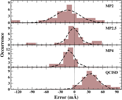
Figure 1: Statistical distribution of the errors on the optimized H$\cdots$H bond length for various methods. The dashed lines indicate interpolated Gaussian curves.

III.2 Interaction energy

The interaction energy of the different dihydrogen complexes, calculated with several wave-function correlated methods, is reported in Tabs. 4 and 5 and Fig. 2.

Table 4: Interaction energy (kcal/mol) for the dihydrogen bond complexes. For each group of systems and the overall set the mean error (ME), mean absolute error (MAE), mean absolute relative error (MARE) and the standard deviation with respect to CCSD(T) data are reported. [Continues in Table 5].

System	MP2	MP2.5	MP4	QCISD	QCISD(T)	CCSD(T)
Hydrides of alkali metals
LiH-HF	14.65	14.40	14.30	13.59	14.04	14.22
LiH-HCl	13.30	12.74	12.23	11.09	11.90	11.88
LiH-HCN	8.70	8.70	8.63	8.14	8.40	8.46
LiH-HCCH	4.25	4.23	4.24	3.80	4.07	4.12
NaH-HF	16.34	15.90	15.59	14.58	15.14	15.33
NaH-HCl	24.77	23.59	22.05	20.39	21.46	21.38
NaH-HCN	8.97	8.88	8.69	7.90	8.28	8.35
NaH-HCCH	4.09	4.00	3.95	3.26	3.66	3.73
ME	0.95	0.62	0.28	-0.59	-0.07
MAE	0.95	0.62	0.28	0.59	0.09
MARE	7.56%	5.21%	2.90%	6.27%	0.96%
Std.Dev.	1.07	0.69	0.19	0.24	0.09
Hydrides of group-3A elements
BH-HF	0.20	0.22	0.48	0.28	0.52	0.52
BH-HCl	0.10	0.05	0.20	-0.11	0.19	0.19
BH-HCN	-0.24	-0.19	-0.01	-0.19	0.03	0.04
BH-HCCH	-0.06	-0.06	0.05	-0.10	0.05	0.05
AlH-HF	6.15	6.02	6.06	5.56	5.90	6.07
AlH-HCl	4.61	4.34	4.19	3.44	3.99	4.03
AlH-HCN	3.00	2.97	3.01	2.59	2.85	2.94
AlH-HCCH	1.38	1.34	1.40	1.01	1.28	1.33
GaH-HF	5.51	5.40	5.44	4.91	5.30	5.48
GaH-HCl	4.40	4.11	3.90	3.12	3.72	3.75
GaH-HCN	2.54	2.51	2.55	2.10	2.39	2.46
GaH-HCCH	0.74	0.68	0.74	0.29	0.62	0.66
ME	0.07	-0.01	0.04	-0.39	-0.06
MAE	0.20	0.14	0.06	0.39	0.06
MARE	90.31%	79.40%	14.19%	103.00%	4.05%
Std.Dev.	0.29	0.19	0.07	0.16	0.06

Table 5: [Continues from Table 4]. Interaction energy (kcal/mol) for the dihydrogen bond complexes. For each group of systems and the overall set the mean error (ME), mean absolute error (MAE), mean absolute relative error (MARE) and the standard deviation with respect to CCSD(T) data are reported.

System	MP2	MP2.5	MP4	QCISD	QCISD(T)	CCSD(T)
Dihydrides of group-2A elements
HBeH-HF	3.43	3.39	3.44	3.14	3.36	3.42
HBeH-HCl	2.35	2.24	2.19	1.81	2.10	2.10
HBeH-HCN	1.92	1.93	1.97	1.77	1.90	1.92
HBeH-HCCH	1.04	1.05	1.09	0.90	1.03	1.05
HMgH-HF	7.02	6.88	6.86	6.38	6.70	6.74
HMgH-HCl	5.05	4.80	4.61	3.92	4.41	4.35
HMgH-HCN	3.64	3.63	3.63	3.27	3.48	3.48
HMgH-HCCH	1.82	1.81	1.84	1.50	1.72	1.73
ME	0.19	0.12	0.11	-0.26	-0.01
MAE	0.19	0.13	0.11	0.26	0.03
MARE	5.40%	3.68%	3.71%	9.83%	0.91%
Std.Dev.	0.24	0.15	0.08	0.10	0.04
Silane
SiH4-HF	1.01	0.98	1.07	0.85	1.02	1.05
SiH4-HCl	0.82	0.74	0.73	0.41	0.67	0.68
SiH4-HCN	0.61	0.60	0.65	0.47	0.61	0.62
SiH4-HCCH	0.34	0.32	0.37	0.19	0.34	0.35
ME	0.02	-0.02	0.03	-0.20	-0.02
MAE	0.05	0.05	0.03	0.20	0.02
MARE	7.22%	6.82%	4.95%	32.17%	2.20%
Std.Dev.	0.08	0.05	0.01	0.05	0.01
Overall performance
ME	0.31	0.18	0.11	-0.38	-0.04
MAE	0.37	0.25	0.12	0.38	0.05
MARE	38.01%	32.85%	7.59%	46.67%	2.26%
Std.Dev.	0.67	0.44	0.14	0.21	0.06

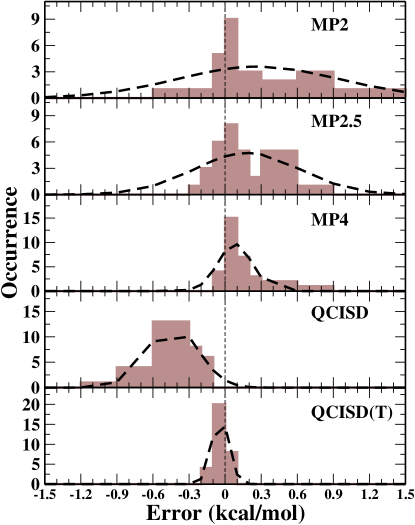
Figure 2: Statistical distribution of the errors on the interaction energy for various methods. The dashed lines indicate interpolated Gaussian curves.

The results show that, as it may be expected, QCISD(T) calculations are very close to CCSD(T) ones, with average differences of the order of 0.06 kcal/mol. This error is close to the expected accuracy of CCSD(T) calculations hobza13 ; feller11 ; feller06 . Thus, the two methods can be considered equally accurate from the practical point of view. Similarly, almost identical results are found for QCISD and CCSD calculations.

Slightly larger deviations from the CCSD(T) reference are found for MP4, which yields a MARE of about 7.5% corresponding to a MAE of 0.12 kcal/mol. Overall, MP4 performs very similarly to QCISD(T) and CCSD(T) for most of the systems. However, for some of the hydrides of alkali metals (e.g. Na–H$\cdots$H–Cl) rather larger errors are found. For these systems the relatively poor performance of MP4 shall be traced back to a worse convergence of the Møller-Plesset perturbative expansion, as indicated by the fact that they show the larger errors also for MP2 and MP2.5. Note that these systems also display a similar behavior for the geometry errors. Furthermore, the MP4 method fails to provide a correct description of the B–H$\cdots$H-CN complex, which results unbound (by -0.01 kcal/mol) at the MP4 level of theory. We note, however, that this is a particularly difficult case, because the reference CCSD(T) interaction energy is only 0.04 kcal/mol. Thus, small inaccuracies in the CCSD(T) results as well as the employed QCISD(T) geometry may play a relevant role in this case, making the comparison uncertain.

All other methods, i.e. the low-level MP2 method including only double excitations, as well as the MP2.5 method and QCISD, including triple corrections, fail to reproduce accurate interaction energies in numerous cases. In particular, they face limitations to describe the hydrides of alkali metals, yielding mean absolute errors larger than 0.6 kcal/mol, and the weakest bonds of the hydrides of the elements of group 3A. In this latter case, all three methods predict incorrectly a negative interaction energy. As a result, the overall performance of MP2, MP2.5, and QCISD is definitely poorer than the one of MP4 and QCISD(T), with a mean absolute relative error that is about five time larger.

III.3 Overall performance

The results of previous subsections indicate that none of the examined wave-function methods is able to yield simultaneously reliable binding energies and H$\cdots$H bond distances, as compared to the reference CCSD(T)/QCISD(T) results, with the exception of MP4, which performs reasonably well for both properties (see Fig. 3).

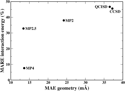
Figure 3: Mean absolute error (MAE) for H$\cdots$H bond length versus the mean absolute relative error (MARE) on interaction energies for several wave-function methods. The most accurate methods shall occupy the left bottom corner of the plot.

Nevertheless, as we mentioned before, MP4 suffers from its inability to describe certain systems, for which it shows errors much above its average. This fact, together with the relatively high computational cost of the MP4 method, contributes to penalize MP4 as a method of choice in the study of dihydrogen interactions and suggests that, when high accuracy is sought, QCISD(T) calculations may be employed instead.

Concerning other, cheaper methods we remark once more that all display several limitations for the calculation of binding energies and/or geometries. However, when computational effort is an issue, the MP2 (or even better the MP2.5) method appears to be the best compromise to achieve reasonable accuracy with a moderate effort. We remark in particular that the MP2.5 method is in fact able to yield results comparable with MP4 for many systems. However, it shows limitations for some specific systems which are more strongly characterized by long-range interactions.

III.4 Energy decomposition analysis

To understand better the nature of the bonding in the different complexes we performed an energy decomposition analysis via SAPT2+3 calculations. The results of this analysis are listed in Table 6, where the electrostatic, exchange, induction and dispersion contributions to the interaction energy are reported. In addition we report, in analogy with Ref. 111, the relative weight of each component, defined as $w=|E_{i}|/\sum_{i}|E_{i}|$, with $E_{i}$ denoting the different interaction energy contributions.

Table 6: Different components of the SPAT2+3 energy (kcal/mol) for the dihydrogen bond complexes and, in parenthesis, their relative weight $w$ in % (see text).

System	Electrostatic		Exchange		Induction		Dispersion		Total
LiH-HF	18.89	(34%)	-20.54	(37%)	11.38	(20%)	4.87	( 9%)	14.60
LiH-HCl	19.11	(26%)	-30.36	(41%)	17.09	(23%)	7.37	(10%)	13.21
LiH-HCN	13.09	(39%)	-12.35	(36%)	5.25	(15%)	3.22	( 9%)	9.21
LiH-HCCH	6.84	(35%)	-7.52	(39%)	2.76	(14%)	2.37	(12%)	4.45
NaH-HF	22.37	(30%)	-28.68	(39%)	16.78	(23%)	6.38	( 9%)	16.85
NaH-HCl	27.18	(18%)	-60.05	(40%)	47.02	(32%)	14.48	(10%)	28.63
NaH-HCN	16.83	(33%)	-20.17	(40%)	8.67	(17%)	4.68	( 9%)	10.01
NaH-HCCH	9.35	(31%)	-13.00	(43%)	4.65	(15%)	3.50	(11%)	4.50
BH-HF	0.38	(5%)	-3.26	(47%)	1.86	(27%)	1.48	(21%)	0.46
BH-HCl	0.82	(10%)	-4.16	(48%)	1.65	(19%)	1.98	(23%)	0.29
BH-HCN	0.04	(1%)	-1.62	(49%)	0.69	(21%)	0.98	(29%)	0.08
BH-HCCH	0.29	(9%)	-1.58	(48%)	0.40	(12%)	1.00	(31%)	0.11
AlH-HF	8.22	(29%)	-11.32	(39%)	5.91	(21%)	3.38	(12%)	6.19
AlH-HCl	7.81	(24%)	-13.99	(43%)	6.24	(19%)	4.41	(14%)	4.46
AlH-HCN	5.84	(30%)	-8.15	(42%)	3.02	(16%)	2.31	(12%)	3.02
AlH-HCCH	3.88	(27%)	-6.29	(44%)	1.70	(12%)	2.31	(16%)	1.60
GaH-HF	8.65	(26%)	-13.94	(41%)	7.18	(21%)	3.95	(12%)	5.85
GaH-HCl	8.37	(22%)	-16.45	(44%)	7.45	(20%)	5.02	(13%)	4.39
GaH-HCN	6.20	(28%)	-9.69	(43%)	3.55	(16%)	3.03	(13%)	3.08
GaH-HCCH	4.80	(25%)	-9.01	(47%)	2.32	(12%)	2.96	(16%)	1.06
HBeH-HF	4.64	(27%)	-6.88	(40%)	3.45	(20%)	2.32	(13%)	3.53
HBeH-HCl	3.80	(24%)	-6.70	(43%)	2.65	(17%)	2.58	(16%)	2.32
HBeH-HCN	2.89	(32%)	-3.48	(38%)	1.26	(14%)	1.49	(16%)	2.16
HBeH-HCCH	1.73	(29%)	-2.40	(40%)	0.61	(10%)	1.23	(21%)	1.17
HMgH-HF	9.45	(30%)	-12.46	(39%)	6.49	(20%)	3.51	(11%)	6.99
HMgH-HCl	8.40	(25%)	-14.13	(43%)	6.36	(19%)	4.33	(13%)	4.96
HMgH-HCN	6.29	(33%)	-7.48	(39%)	2.81	(15%)	2.44	(13%)	4.06
HMgH-HCCH	3.88	(30%)	-5.47	(42%)	1.55	(12%)	2.06	(16%)	2.02
SiH4-HF	0.88	(11%)	-3.39	(43%)	1.99	(25%)	1.61	(20%)	1.10
SiH4-HCl	1.13	(13%)	-4.08	(45%)	1.69	(19%)	2.11	(23%)	0.84
SiH4-HCN	0.75	(15%)	-2.20	(43%)	0.92	(18%)	1.29	(25%)	0.77
SiH4-HCCH	0.55	(14%)	-1.76	(45%)	0.47	(12%)	1.18	(30%)	0.43

We see that for most systems the energy decomposition describes a bonding behavior quite similar to conventional hydrogen bonds hoja14 , despite for the present dihydrogen bonds we observe in general a slightly more important role of electrostatic and induction terms and a reduced influence of the dispersion contributions. In fact in all cases the largest component of the interaction energy is the exchange one, which weights about 40% and is repulsive. In most cases the second largest contribution is given by the attractive electrostatic interaction, which has a weight of 25-30%. Finally, the induction and dispersion terms provide further, but less important, contributions to the interaction energy, having on average weights of about 20% and 10%, respectively.

We note, however, that for some systems, especially in the set the of hydrides of group-3A elements and the complexes of silane, the importance of dispersion interactions is much larger, being eventually the second contribution, after exchange, to the total interaction energy. These systems shall thus be regarded as laying at the boundary between dihydrogen bond and dispersion complexes. This explains why most of these systems display very low interaction energies and consequently can be accurately described only by the higher level approaches.

IV Density functional theory calculations

In this section we report an assessment of some popular DFT functionals for the description of the equilibrium geometry and the interaction energy of the dihydrogen complexes studied in the previous section. We remark that, due to the huge number of existing XC functionals, this study is not intended as an exhaustive investigation, but rather aims to provide a general feeling of the performance that can be expected from DFT. In particular, we did not considered Van der Waals corrected functionals. In fact, an analysis of the many different existing techniques for the treatment of Van der Waals forces in the DFT framework requires a large effort and deserves a separate investigation (see for example Refs. 3; 113; 114; 115). Moreover, the analysis of the results concerning complexes with very different energies and bonding nature will be very complicated and deserves separate studies. For these reasons we removed from the test set considered in the following analysis those complexes where dispersion interactions are particularly relevant, which are the ones that have in Table 6 the weight of dispersion contributions exceeding 20% (i.e. all BH- and silane complexes as well as HBeH–HCCH; note that for most of these systems dispersion is also the second biggest contribution in the interaction energy).

IV.1 Equilibrium H$\cdots$H bond distance

Analyzing the performance of DFT functionals for the H$\cdots$H bond distance we found that the distribution of the errors is spread over a quite large range, covering an interval of about $\pm$200 mÅ for all the functionals with even larger errors for some systems. Moreover, a marked tendency towards the overestimation of the bond distance is observable in general. This situation implies that the performance of different functionals can not be measured by computing, as usual, mean (absolute) (relative) errors, because for such a broad distribution of data the average will contain little information. Thus, we prefer to report in Fig. 4, for each functional, the histogram of the cumulative number of systems with error below a certain value. That is, for each functional we define $\Delta R_{H-H}^{i}$ the absolute error on the H$\cdots$H bond length for the $i$-th complex and we consider the quantity

$$N(\Delta R_{H-H})=\sum_{i=1}^{23}f(\Delta R_{H-H}^{i};\Delta R_{H-H})\ ,$$ (1)

where $f(\Delta R_{H-H}^{i};\Delta R_{H-H})=1$ if $\Delta R_{H-H}^{i}\leq\Delta R_{H-H}$ and 0 otherwise. Furthermore, to obtain a more quantitative evaluation of the performance of different functionals we consider the indicator $\Lambda=(1-\epsilon)/\epsilon$, where $\epsilon$ is the integrated error

$$\epsilon=\frac{1}{23R_{max}}\int_{0}^{R_{max}}N(x)dx\ ,$$ (2)

with $R_{max}$ being fixed to 300 mÅ. Given that $R_{max}$ is chosen such that $N(R_{max})=N_{max}$, the indicator $\Lambda$ shows how fast the function $N$ grows to its maximum (all curves in Fig. 4 are roughly fitted by $N(x)\propto x^{\Lambda}$). Therefore, for a perfect functional we would have $\Lambda=0$, whereas for a very poor functional $\Lambda\rightarrow\infty$.

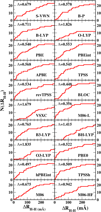
Figure 4: Cumulative number $N(\Delta R_{H-H})$ of systems with error lower or equal than $\Delta R_{H-H}$ for different XC functionals. The integrated error $\Lambda$ is also reported (see text for details).

The plots of Fig. 4 show that most functionals perform rather poorly for the H$\cdots$H equilibrium distance. In fact, in most cases errors below 25 mÅ are obtained only for few systems and even errors below 100 mÅ are not very common. According to our analysis the best performance is given by the M06-L functional ($\Lambda=0.356$), which yields 60% of the complexes with an error less than 50 mÅ. Relatively good results are obtained also from PBE, PBEint, and APBE among the GGAs, BLOC among the meta-GGAs, and hPBEint among the hybrids. Very poor results are given, on the other hand, by O-LYP, VSXC, BH-LYP, O3-LYP, and M06-HF, that all make worse than the simple local density approximation. Note that also the popular B3-LYP functional displays a rather disappointing behavior being similar with S-VWN. Indeed, the inclusion of small fraction of Hartree-Fock exchange into the hybrids seems to bring in general a slight improvement of the performance, whereas functionals including a large amount of Hartree-Fock exchange display in general poor results (see also later on).

IV.2 Interaction energy

The mean absolute (relative) errors on the interaction energies computed with different XC functionals are reported in Table 7.

Table 7: Mean absolute errors (kcal/mol) and mean absolute relative errors (in parenthesis) on the interaction energy of different groups of dihydrogen bond complexes. The overall errors are also reported in the last column.

Functional	alkali metals			group 3A			Group 2A			overall
LDA/GGA functionals
S-VWN	3.45	(35.35%)		3.13	(123.21%)		2.08	(65.89%)		2.89	(76.75%)
B-P	0.61	(7.87%)		0.61	(22.24%)		0.36	(15.74%)		0.53	(15.56%)
B-LYP	1.13	(14.60%)		0.51	(24.50%)		0.48	(19.72%)		0.70	(19.80%)
O-LYP	2.52	(31.71%)		1.38	(75.37%)		1.55	(55.45%)		1.80	(55.02%)
PBE	0.52	(3.63%)		0.95	(29.51%)		0.35	( 9.41%)		0.62	(14.80%)
PBEint	0.70	(4.99%)		0.91	(27.06%)		0.38	(10.76%)		0.67	(14.78%)
APBE	0.41	(3.77%)		0.77	(22.27%)		0.27	(7.55%)		0.49	(11.64%)
meta-GGA functionals
TPSS	0.64	(4.84%)		0.63	(17.90%)		0.28	( 8.29%)		0.52	(10.65%)
revTPSS	0.16	(1.98%)		0.44	(12.50%)		0.20	( 6.99%)		0.27	( 7.37%)
BLOC	0.97	(9.38%)		0.92	(30.99%)		0.44	(11.46%)		0.78	(17.83%)
VSXC	0.50	(4.00%)		0.29	(10.72%)		0.17	(5.67%)		0.32	( 6.95%)
M06-L	1.07	(10.84%)		0.62	(19.98%)		0.28	( 9.70%)		0.65	(13.77%)
hybrid functionals
B3-LYP	0.50	(7.16%)		0.36	(17.11%)		0.30	(13.03%)		0.39	(12.62%)
BH-LYP	0.24	(3.07%)		0.25	(12.72%)		0.20	( 8.40%)		0.23	( 8.25%)
O3-LYP	1.83	(23.58%)		1.08	(59.95%)		1.22	(44.14%)		1.37	(43.25%)
PBE0	0.72	(5.92%)		0.51	(14.40%)		0.20	(5.42%)		0.48	( 8.81%)
hPBEint	0.80	(6.18%)		0.64	(18.50%)		0.28	( 7.96%)		0.57	(11.18%)
hybrid meta-GGA functionals
TPPSh	0.66	(5.20%)		0.50	(13.72%)		0.24	( 7.62%)		0.47	( 9.04%)
M06	0.72	(8.06%)		0.60	(22.27%)		0.14	(3.58%)		0.49	(11.74%)
M06-HF	0.43	(5.00%)		0.56	(31.18%)		0.62	(23.07%)		0.54	(20.20%)

The overall performance of all functionals is in line with that obtained for conventional hydrogen bonds hb06 , with average errors mostly included in the range 0.3-0.5 kcal/mol. The best functionals in Table 7 turn out to be BH-LYP (MAE=0.23 kcal/mol, MARE=8.3%) and revTPSS (MAE=0.27 kcal/mol, MARE=7.4%); amongst the GGAs the best performance is shown by APBE with a MAE=0.49 kcal/mol (MARE=11.6%). Nevertheless, all functionals, but S-VWN, O-LYP and O3-LYP, perform quite similarly on average. Slightly larger differences are observed considering individual groups of complexes. However, a clear trend cannot be established. Nevertheless, we can note that in general meta-GGA functionals yield the best results and the most uniform description of different systems also among different classes. The inclusion of Hartree-Fock exchange in hybrids, appears to slightly improve the description of the dihydrides of group 2A and 3A elements, whereas it yields a little worsening for the complexes of the alkali metals.

To try to rationalize better this behavior we consider a density analysis of some representative complexes. Thus, in the upper panel of Fig. 5 we report a plot of the reduced gradient $s=|\nabla n|/[(4(3\pi^{2})^{2/3}n^{4/3}]$ as a function of the electron density ($n$) times the second eigenvalue of the electron-density Hessian ($\lambda_{2}$). This is the NCI indicator nci ; nci2 which is able to characterize different kinds of non-covalent interactions. Inspection of the plot shows that all the systems are characterized by a clear hydrogen-like bonding pattern, although with varying strengths, without significant van der Waals signatures even for the weakest complexes (e.g. GaH-HCCH). This fact confirms that our selection of systems with (almost) no dispersion character, performed on the basis of the SAPT energy decomposition is in fact efficient. Moreover, it suggests that a deeper analysis can be brought on on the basis of some semilocal density indicators.

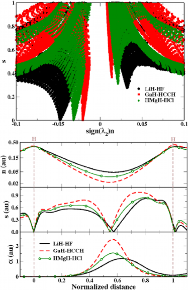
Figure 5: Plot of the NCI indicator nci ; nci2 (upper panel) and of several density parameters as functions of the normalized bond distance (lower panel) for the LiH-HF, LiH-HCCH, and BH-HCCH complexes. See text for details.

In the lower panel of Fig. 5 we report the plot of some important density indicators in the bond region of three exemplary complexes. Namely, we plot the electron density, the reduced gradient which denotes regions where the density is slowly- or rapidly-varying, and the meta-GGA ingredient $\alpha=(\tau-\tau^{W})/\tau^{TF}$ where $\tau$ is the positive defined kinetic energy density, $\tau^{W}=|\nabla n|^{2}/(8n)$ is the von Weizsäcker kinetic energy density, and $\tau^{TF}=(3/10)(3\pi^{2})^{2/3}n^{5/3}$ is the Thomas-Fermi kinetic energy. The latter distinguishes between iso-orbital regions and slowly-varying regions. In the plot, for each complex, the distance is normalized to the H$\cdots$H bond distance, so that the curves are all comparable.

The figure indicates how difficult may be for a semilocal DFT functional to differentiate between various complexes. In fact, despite the three complexes considered for the plots have interaction energies that vary from 14.22 (LiH-HF) to 0.66 kcal/mol (GaH-HCCH), they display only minor differences as to what concerns the density and the reduced gradient $s$ in the bond region. In particular, whereas the density shows a weak trend with the interaction strength (complexes with strongest binding have a slightly larger density in the bond) the reduced gradient $s$ is very similar in all cases. On the other hand, important differences between the various complexes can be observed by inspecting the meta-GGA indicator $\alpha$. This helps to explain the better performance of meta-GGA functionals with respect to GGA ones in terms of their superior ability to discriminate the nature of the different bonding patterns.

Additionally, Fig. 5 shows that for all complexes the bonding region is fundamentally a slowly-varying density region, since $s\lessapprox 0.8$ there. This explains the failure of the functionals based on the OPTX exchange optx (e.g. O-LYP, O3-LYP) which even fail to recover the local density approximation limit. Nevertheless, it must be noted that the proper slowly-varying density limit is only observed in the strongest dihydrogen complexes (e.g. LiH-HF) where $\alpha\approx 1$ in the bond. For the complexes displaying a weakest interaction instead $\alpha$ is quite larger indicating that the bonding region is an evanescent region for the density characterized by the contribution of many orbitals (otherwise $\alpha$ would be zero as in 1 or 2 electron systems). This situation resembles the interaction of two closed-shell atoms, and cannot be easily described at the semilocal level of theory. Thus, we have an additional element to explain the superiority of meta-GGA functionals in this context (group-2A and especially group-3A complexes). Furthermore, this finding strongly helps to rationalize the fact that the inclusion of Hartree-Fock exchange generally improves the performance of the functionals for the description of interaction energies (see also next subsection), especially in the case of complexes of group-3A and group-2A elements. In fact, the inclusion of non local exchange contributions is likely to improve the description of non local interactions between the two weakly overlapping densities.

IV.3 Hybrid functionals

To investigate in some more detail the role of nonlocal Hartree-Fock exchange in hybrid functionals we consider in this subsection a couple of model hybrid XC functionals of the form

$$E_{xc}^{\mathrm{hybrid}}=\beta_{HF}E_{x}^{HF}+(1-\beta_{HF})E_{x}^{DFT}+E_{c}^{DFT}\ ,$$ (3)

where $\beta_{HF}$ is a parameter, $E_{x}^{HF}$ is the Hartree-Fock exchange energy, $E_{x}^{DFT}$ is some semilocal DFT exchange functional, and $E_{c}$ is a DFT correlation functional. A similar model was used in Refs. 119; 120. In this work we consider DFT=PBE, BLOC and we compute the MAE on interaction energies as well the value of the indicator $\Lambda$ while $\beta_{HF}$ is varied between 0 and 1. The results of these calculations are reported in Fig. 6.

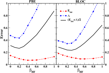
Figure 6: Indicator for geometry errors $\Lambda$ and the mean absolute relative error on interaction energies for different values of the fraction of Hartree-Fock exchange in functionals of the form given by Eq. (3) with DFT=PBE (left) and DFT=BLOC (right). In each panel we also report the global performance computed as the average between $\Lambda$ and the MAE.

The plot shows that for both PBE and BLOC a similar behavior is obtained (which is common also to other functionals not shown), with a decrease of the errors for rather small fractions of Hartree-Fock exchange and a worsening of the performance when a larger amount of nonlocal exchange is considered. This trend is similar for both the geometry and interaction energy errors. However, for the former case the benefits are observed only for small fractions of Hartree-Fock exchange, while a significant increase of the errors is obtained for $\beta_{HF}>0.4$; For interaction energies instead a larger fraction of Hartree-Fock exchange is required for better performance and no dramatic worsening of the results is achieved even for $\beta_{HF}=1$. Thus, all in all we can estimate both functionals to have a “best” average performance at a moderately small fraction of Hartree-Fock exchange mixing, i.e. at about 20% (we denote these “best” hybrids hPBE with $\beta_{HF}=0.20$ and hBLOC with $\beta_{HF}=0.25$).

We note however, that the results shown in Fig. 6 are only an average over the various systems that display in general very different behaviors. For example, for interaction energies the inclusion of Hartree-Fock exchange has a quite different effect on complexes of the alkali metals than on weaker dihydrogen complexes. In the former case in fact GGA functionals generally overestimate the interaction energy and the addition of Hartree-Fock exchange further increases this overestimation. Thus, the error usually increases with $\beta_{HF}$. On the other hand, for complexes of the elements of group 3A, the GGA functionals mostly provide an overestimation of the interaction energy but the inclusion of exact exchange reduces it, so that small errors are generally obtained at rather large values of $\beta_{HF}$. Finally, a mixture of these two trends is observable for complexes of the group-2A elements. Therefore, although the inclusion of a moderate fraction of Hartree-Fock exchange can be positive for DFT calculations, it must be kept in mind that a good balance between all the effects and for different systems, is difficult to achieve. Thus, caution must be taken before extrapolating general conclusions to individual cases.

In consideration of the last comments, we complete this section by reporting in Tab. 8 the mean absolute relative errors for interaction energies as obtained by several range-separated hybrid functionals.

Table 8: Mean absolute errors (kcal/mol) and mean absolute relative errors (in parenthesis) on the interaction energy of different groups of dihydrogen bond complexes as computed with everal range-separated DFT functionals. The overall errors are also reported in the last column.

Functional	alkali metals			group 3A			Group 2A			overall
CAM-B3LYP	0.28	(3.35%)		0.33	(12.82%)		0.24	(9.28%)		0.29	(8.45%)
LC-BLYP	0.72	(6.96%)		0.99	(33.14%)		0.59	(17.21%)		0.77	(19.18%)
$\omega$B97	0.83	(10.04%)		0.49	(19.31%)		0.48	(15.98%)		0.61	(15.07%)
$\omega$B97X	0.77	(9.45%)		0.50	(20.57%)		0.45	(15.05%)		0.58	(15.02%)

The table shows that range-separated hybrid functionals perform generally very well for the complexes under exam. However, they bring no clear advantage with respect to global hybrid functionals (CAM-B3LYP is a little better that B3-LYP but worst than BH-LYP; all other functionals are slightly worst that all global hybrids except O3-LYP). Thus, the separation between short- and long-range exchange terms does not appear to be a crucial factor in the treatment of dihydrogen bonds.

On the other hand, we saw that the functionals incorporating a larger amount of exact exchange perform better than others for the description of interaction energies. This issue can be possibly related, to a smaller delocalization error of these functionals.

IV.4 Overall performance

As we saw a DFT functional can produce results of different quality when the interaction energy or the accuracy of the description of the H$\cdots$H bonds are considered. This is an important issue because in practical applications both the structure and the interaction energy must be accurately described. Therefore, a well balanced description must be preferred to a situation where one property is described very well but the other is not. This assessment is presented in Fig. 7, where we report for selected functionals the value of the indicator $\Lambda$ for the geometry versus the mean absolute relative error on the interaction energies. Note that in the figure, for interaction energy, both MAREs obtained using QCISD(T) reference geometries (top panel) and MAREs obtained relaxed DFT geometries (bottom panel) are considered. The former are in fact more closely related to the discussion of previous sections, whereas the latter are more appropriate for an assessment of practical calculations where the geometry and the energy are likely calculated at the same level of theory. Nevertheless, both cases show very similar trends, while the most evident difference is that with relaxed DFT geometries the MARE on interaction energy is generally increased. The most accurate functionals are thus located in the bottom left corner of the plot, whereas the top right corner will host the worst performing functionals. We note that, in this case, the MARE gives a more realistic statistical assessment of a given functional than the MAE, because the interaction energies of the benchmark systems span a considerable range of interaction energies going from 0.52 kcal/mol 21.38 kcal/mol.

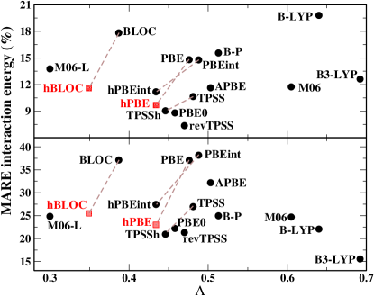
Figure 7: Indicator for geometry errors $\Lambda$ versus the mean absolute relative error (MARE) on interaction energies for selected DFT functionals. The top panel report MAREs computed with QCISD(T) geometries; the bottom panel reports the MAREs computed using relaxed geometries. In each panel the most accurate methods shall occupy the left bottom corner of the plot.

Inspection of the figure shows that the overall performance of DFT functionals is quite erratic. Nevertheless, there exist a group of functionals, including the meta-GGAs revTPSS and M06-L as well as the hybrids TPSSh, PBE0, and hPBEint, which perform all quite well, despite none of them can be simultaneously well accurate for both geometries and energies. We can rate these functionals as the most reliable for applications on dihydrogen bonds. On the other hand, several functionals, mainly GGAs such as PBE and APBE, lay in the central part of the figure, showing that they display a moderate accuracy for both geometries and interaction energies. This result seems to contrast with the fact that they are instead quite good for conventional hydrogen bonds mukappa . However, the results of previous sections indicate that the overall performance of these functionals is penalized by their inability to describe some cases (typically the weakest bonds), whereas they can be a good choice for complexes where a larger overlap of the fragment densities is present. We remark finally, that in general the performance of functionals can be improved by the inclusion of a small fraction of Hartree-Fock exchange in a hybrid scheme, as shown by the hPBE and hBLOC points reported in Fig. 7 (compare also PBEint and hPBEint).

V Conclusions

We performed a benchmark study of dihydrogen bond complexes. Thus, we were able to define a set of reference geometries and interaction energies for a representative set of small complexes. This set can be used in future assessments of methods for the description of dihydrogen interactions.

In this work we have tested, against the benchmark, a few wave-function correlated methods. We found that second-order methods (i.e. MP2 and QCISD) are rather accurate, giving mean absolute errors of few tens of mÅ for H$\cdots$H bond lengths and about 0.4 kcal/mol for interaction energies. Nevertheless, high accuracy appears to be out of reach for these approaches. In particular, the MP2 method, although displaying a slightly better average performance, generally shows a broad distribution of the errors. Thus, it must be employed with caution because relatively large errors can be obtained for some cases. For this reason the use of the more reliable MP2.5 method may seem a good compromise between accuracy and computational cost. Alternatively, we must acknowledge the possibility of considering spin-resolved MP2 approaches (e.g. SCS- or SOS-MP2) scsmp2 ; scsmp2_rev ; sosmp2 , eventually using a specialized parameterization scs_noncov ; scspccp , which already showed an encouraging performance for non-covalent interactions scsmp2_rev ; scs_noncov ; scspccp . Nevertheless, to this end a careful testing against the benchmark must be considered in future work.

Finally, we had a survey on the performance of some popular density functional methods, to understand the level of accuracy that may be expected by such calculations. Interestingly, we found that for the H$\cdots$H bond length none of the functionals was able to yield reliable results and a general overestimation of the bond distance is found instead. On the other hand, most functionals provide quite accurate results for the interaction energies, yielding a mean absolute error lower than 0.5 kcal/mol, which is comparable to the MP2 and QCISD results. However, the quality of the interaction energies for single cases varies quite significantly, reflecting the broad differences between the various dihydrogen complexes. In fact, a detailed analysis of the density and its related descriptors in the bonding region of several complexes revealed that the different features of the various dihydrogen bonds can be hardly described at the semilocal level of the theory. Thus, for a reliable description of different complexes it appears necessary to revert to higher rung functionals making use of the occupied Kohn-Sham orbitals (i.e. meta-GGAs and/or hybrids).

In conclusion, great caution shall be used when performing DFT calculations on complexes displaying dihydrogen bonding because DFT functionals appear generally unable to fully describe the complex balancing of effects present in these systems. Nevertheless, meta-GGA functionals and especially hybrids seem to give higher reliability in this sense. Finally, some attention must be payed to the possible mismatch between the description of different properties and functionals yielding a more balanced description of different properties (see Fig. 7) shall be possibly preferred.

VI Acknowledgments

We thank TURBOMOLE GmbH for providing the TURBOMOLE program package.

References

- (1) Sherrill, C. D. Acc. Chem. Res. 2013, 46, 1020.
- (2) Hohenstein, E. G.; Sherrill, C. D. WIREs Comput Mol Sci 2012 2, 304.
- (3) Burns, L. A.; Vázquez-Mayagoitia, A.; Sumpter, B. G.; Sherrill, C. D. J. Chem. Phys. 2011 134, 084107.
- (4) Thanthiriwatte, K. S.; Hohenstein, E. G.; Burns, L. A.; Sherrill, C. D. J. Chem. Theory Comput. 2011 7, 88.
- (5) Sherrill, C. D.; Takatani, T.; Hohenstein, E. G. J. Phys. Chem. A 2009 113, 10146.
- (6) Dubecký, M.; Jurečka, P.; Derian, R.; Hobza, P.; Otyepka, M.; Mitas, L. J. Chem. Theory Comput. 2013 9, 4287.
- (7) Sedlak, R.; Janowski, T.; Pitoňák, M.; Řezáč, J.; Pulay, P.; Hobza, P. J. Chem. Theory Comput. 2013 9, 3364.
- (8) Řezáč, J.; Hobza, P. J. Chem. Theor. Comput. 2013 9, 2151.
- (9) Melicherčík, M.; Pitoňák, M.; Kellö, V.; Hobza, P.; Neogrády, P. J. Chem. Theory Comput. 2013 9, 5296.
- (10) Riley, K. E.; Hobza, P. Phys. Chem. Chem. Phys. 2013 15, 17742.
- (11) Riley, K. E.; Murray, J. S.; Fanfrlík, J.; Řezáč, J.; Solá, R. J.; Concha, M. C.; Ramos, F. M.; Politzer, P. Journal of Molecular Modeling 2013 19, 4651.
- (12) Zhao, Y.; Truhlar, D. G. J. Chem. Theory Comput. 2007, 3, 289.
- (13) Zhao, Y.; Truhlar, D. G. J. Chem. Theory Comput. 2006 2, 1009.
- (14) Johnson, E. R.; Otero de la Roza, A.; Dale, S. G.; Di Labio, G. A. J. Chem. Phys. 2013 139, 214109.
- (15) Otero de la Roza, A.; Johnson, E. R. J. Chem. Phys. 2013 138, 204109.
- (16) Johnson, E. R.; Salamone, M.; Bietti, M.; Di Labio, G. A. J. Phys. Chem. A. 2013 117, 947.
- (17) Contreras-García, J.; Johnson, E. R.; Keinan, S.; Chaudret, R.; Piquemal, J.-P.; Beratan,D. N.; Yang, W. J. Chem. Theory Comput. 2011 7, 625.
- (18) Johnson, E. R.; Keinan, S.; Mori-Sánchez, P.; Contreras-García, J.; Cohen, A. J.; Yang, W. J. Am. Chem. Soc. 2010 132, 6498.
- (19) Grabowski, S. J. Journal of Molecular Modeling 2013 19, 4713.
- (20) Hobza, P.; Müller-Dethlefs, K.; Jordan, K. D.; Lim, C. Non-Covalent Interactions: Theory and Experiment; Royal Society of Chemistry: London, 2009.
- (21) Jeffrey, G. A. An Introduction to Hydrogen Bonding; Oxford University Press: USA, 1997.
- (22) Grabowski, S. J. Hydrogen Bonding - New Insights; Springer: Dordrecht, 2006.
- (23) Kollman, P. A.; Allen, L. C. Chem. Rev. 1972, 72, 283.
- (24) Zhao, G.-J.; Han, K. L. Acc. Chem. Res. 2012 45, 404.
- (25) Grabowski, S. J. Chem. Rev. 2011 111, 2597.
- (26) Li, X.-Z.; Walker, B.; Michaelides, A. Proc. Natl. Accad. Soc. 2011 108, 6369.
- (27) Contreras-García, J.; Yang, W.; Johnson, E. R. J. Phys. Chem. A. 2011 115, 12983.
- (28) Johnson, E. R.; Di Labio, G. A. Interdiscipl. Sci. - Comput. Life. Sci. 2009 1, 133.
- (29) Grabowski, S. J. Phys. Chem. Chem. Phys. 2013 15, 7249.
- (30) Fuster, F.; Grabowski, S. J. J. Phys. Chem. A 2011 115, 10078.
- (31) Bakhmutov, V. I. Dihydrogen Bonds: Principles, Experiments, and Applications; John Wiley & Sons, Inc.: Hoboken, New Jesrsey, 2008.
- (32) Custelcean, R.; Jackson, J. E. Chem. Rev. 2001 101, 1963.
- (33) Grabowski, S. J.; Sokalski, W. A.; Leszczynski, J. J. Phys. Chem. A 2004 108, 5823.
- (34) Hu, S.-W.; Wang, Y.; Wang, X.-Y.; Chu, T.-W.; Liu, X.-Q. J. Phys. Chem. A 2004 108, 1448.
- (35) Hayashi, A.; Shiga, M.; Tachikawa, M. Chem. Phys. Lett. 2005 410, 54.
- (36) Solimannejad M.; Scheiner, S. J. Phys. Chem. A 2005 109, 6137.
- (37) Alkorta, I.; Zborowski, K.; Elguero, J.; Solimannejad, M. J. Phys. Chem. A 2006 110, 10279.
- (38) Solimannejad M.; Alkorta, I. Chem. Phys. 2006 324, 459.
- (39) Solimannejad M.; Boutalib, A. Chem. Phys. 2006 320, 275.
- (40) Yao A.; Ren, F. Comput. Theor. Chem. 2011 963, 463.
- (41) Li, Y.; Zhang, L.; Du, S.; Ren, F.; Wang, W. Comput. Theor. Chem. 2011 977, 201.
- (42) Meng, Y.; Zhou, Z.; Duan, C.; Wang, B.; Zhong, Q. J. Mol. Struct. (Theochem) 2005 713, 135.
- (43) Filippov, O. A.; Filin, A. M.; Tsupreva, V. N.; Belkova, N. V.; Lledos, A.; Uiaque, G.; Epstein, L. M.; Shubina, E. S. Inorg. Chem. 2006 45, 3086.
- (44) Hugas, D.; Simon, S.; Duran, M. J. Phys. Chem. A 2007 111, 4506 (2007).
- (45) Guo, J.; Shi, V.; Ren, F.; Cao, D.; Zhang, Y. J. Mol. Model. 2013 19, 3153.
- (46) Li, B.; Shi, W.; Ren, F. Comput. Theor. Chem. 2013 1020, 81.
- (47) Grabowski, S. J. J. Phys. Org. Chem. 2013, 26, 452.
- (48) Filippov, O. A.; Filin, A. M.; Belkova, N. V.; Tsupreva, V. N.; Smirnova, Y. V.; Sivaev, I. B.; Epstein, L. M.; Shubina, E. S. J. Mol. Struct. 2006 790, 114.
- (49) Zhang, H.; Li, X.; Tang, Y. Front. Phys. 2011 6, 213.
- (50) Sandhya K. S.; Suresh, C. H. Dalton Trans. 2012 41, 11018.
- (51) Flener Lovitt, C.; Frenking, G.; Girolami, G. S. Organometallics 2012 31, 4122.
- (52) Yang, X. J. Clust. Sci. 2012 23, 703.
- (53) Grabowski, S. J. J. Phys. Chem. A 2000 104, 5551.
- (54) Raghavachari, K.; Trucks, G. W.; Pople, J. A.; Head-Gordon, M. Chem. Phys. Lett. 1989 157, 479.
- (55) Pople, J. A.; Head-Gordon, M.; Raghavachari, K. J. Chem. Phys. 1987 87, 5968.
- (56) Gauss J.; Cremer, D. Chem. Phys. Lett. 1988 150, 280.
- (57) Salter, E. A.; Trucks, G. W.; Bartlett, R. J. J. Chem. Phys. 1989 90, 1752.
- (58) Møller C.; Plesset, M. S. Phys. Rev. 1934 46, 0618.
- (59) Head-Gordon, M.; Pople, J. A.; Frisch, M. J. Chem. Phys. Lett. 1988 153, 503.
- (60) Pitoňák, M.; Neogrády, P.; Černý, J.; Grimme, S.; Hobza, P. ChemPhysChem 2009 10, 282.
- (61) Raghavachari K.; Pople, J. A. Int. J. Quantum Chem. 1978 14, 91.
- (62) Hohenstein, E. G.; Sherrill, C. D. J. Chem. Phys. 2010 133, 014101.
- (63) Slater, J. C. Phys. Rev. 1951 81, 385.
- (64) Dirac, P. A. M. Proc. Royal Soc. (London) A 1929 123, 714.
- (65) Vosko, S. H.; Wilk, L.; Nusair, M. Can. J. Phys. 1980 58, 1200.
- (66) Becke, A. D. Phys. Rev. A 1988 38, 3098.
- (67) Perdew, J. P. Phys. Rev. B 1986 33, 8822.
- (68) Lee, C.; Yang, W.; Parr, R. G. Phys. Rev. B 1988 37, 785.
- (69) Handy N. C.; Cohen, A. J. Mol. Phys. 2001 99, 403.
- (70) Perdew, J. P.; Burke, K.; Ernzerhof, M. Phys. Rev. Lett. 1996 77, 3865.
- (71) Fabiano, E.; Constantin, L. A.; Della Sala, F. Phys. Rev. B 2010 82, 113104.
- (72) FORTRAN90 routines are freely available at http://www.theory-nnl.it/software.php; accessed on April 2014.
- (73) Constantin, L. A.; Fabiano, E.; Laricchia, S.; Della Sala, F. Phys. Rev. Lett. 2011 106, 186406.
- (74) Tao, J.; Perdew, J. P.; Staroverov, V. N.; Scuseria, G. E. Phys. Rev. Lett. 2003 91, 146401.
- (75) Perdew, J. P.; Ruzsinszky, A.; Csonka, G. I.; Constantin, L. A.; Sun, J. Phys. Rev. Lett. 2009 103, 026403; Phys. Rev. Lett. 2011 106, 179902.
- (76) Constantin, L. A.; Fabiano, E.; Della Sala, F. J. Chem. Theory Comput. 2013 9, 2256.
- (77) Constantin, L. A.; Fabiano, E.; Della Sala, F. Phys. Rev. B 2012 86, 035130.
- (78) Constantin, L. A.; Fabiano, E.; Della Sala, F. Phys. Rev. B 2013 88, 125112.
- (79) Van Voorhis, T.; Scuseria, G. E. J. Chem. Phys. 1998 109, 400.
- (80) Zhao Y.; Truhlar, D. G. J. Chem. Phys. 2006 125, 194101.
- (81) Becke, A. D. J. Chem. Phys. 1993 98, 5648.
- (82) Stephens, P. J.; Devlin, F. J.; Chabalowski, C. F.; Frisch, M. J. J. Phys. Chem. 1994 98, 11623.
- (83) Becke, A. D. J. Chem. Phys. 1993 98, 1372.
- (84) Cohen A. J.; Handy, N. C. Mol. Phys. 2001 99, 607.
- (85) Adamo, C.; Barone, V. J. Chem. Phys. 1999 110, 6158.
- (86) Fabiano, E.; Constantin, L. A.; Della Sala, F. Int. J. Quantum Chem. 2013 113, 673.
- (87) Staroverov, V. N.; Scuseria, G. E.; Tao, J.; Perdew, J. P. J. Chem. Phys. 2003 119, 12129.
- (88) Zhao Y.; Truhlar, D. G. Theor. Chem. Acc. 2008 120, 215.
- (89) Zhao Y.; Truhlar, D. G. J. Phys. Chem. A 2006 110, 13126.
- (90) Yanai, T.; Tew, D. P.; Handy. N. C. Chem. Phys. Lett. 2004 393, 51.
- (91) Tawada, Y.; Tsuneda, T.; Yanagisawa, S.; Yanai, T.; Hirao. K. J. Chem. Phys. 2004 120, 8425.
- (92) Chai, J.-D.; Head-Gordon. M. J. Chem. Phys. 2008 128, 084106.
- (93) Dunning Jr., T. H. J. Chem. Phys. 1989 90, 1007.
- (94) Woon D. E.; Dunning Jr., T. H. J. Chem. Phys. 1993 98, 1358.
- (95) Kendall, R. A.; Dunning Jr., T. H.; Harrison, R. J. J. Chem. Phys. 1992 96, 6796.
- (96) Danovich, D.; Shaik, S.; Neese, F.; Echeverría, J.; Aullón, G.; Alvarez S. J. Chem. Theory Comput. 2013 9, 1977.
- (97) Halkier, A.; Helgaker, T.; Jørgensen, P.; Klopper, W.; Koch, H.; Olsen, J.; Wilson, A. K. Chem. Phys. Lett. 1998 286, 243.
- (98) Fabiano, E.; Della Sala, F. Theor. Chem. Acc. 2012 131, 1278.
- (99) East, A. L. L.; Allen, W. D. J. Chem. Phys. 1993 99, 4638.
- (100) Csaszar, A. G.; Allen, W. D.; Schaefer, H. F. J. Chem. Phys. 1998 108, 9571.
- (101) Burns, L. A.; Marshall, M. S.; Sherrill, C. D. J. Chem. Theory Comput. 2014 10, 49.
- (102) Mackie, I. D.; DiLabio, G. A. J. Chem. Phys. 2011 135, 134318.
- (103) Feller, D.; Peterson, K. A.; Grant Hill, J. J. Chem. Phys. 2011 135, 044102.
- (104) Weigend, F.; Furche, F.; Ahlrichs, R. J. Chem. Phys. 2003 119, 12753.
- (105) Weigend, F.; Ahlrichs, R. Phys. Chem. Chem. Phys. 2005 7, 3297.
- (106) Boys S. F.; Bernardi, F. Mol. Phys. 1970 19, 553.
- (107) TURBOMOLE, V6.3; TURBOMOLE GmbH: Karlsruhe, Germany, 2011. Available from http://www.turbomole.com (accessed April 2014).
- (108) Neese, F. WIREs Comput. Mol. Sci. 2012 2, 73.
- (109) Turney, J. M.; Simmonett, A. C.; Parrish, R. M.; Hohenstein, E. G.; Evangelista, F.; Fermann, J. T.; Mintz, B. J.; Burns, L. A.; Wilke, J. J.; Abrams, M. L.; Russ, N. J.; Leininger, M. L.; Janssen, C. L.; Seidl, E. T.; Allen, W. D.; Schaefer, H. F.; King, R. A.; Valeev, E. F.; Sherrill, C. D.;Crawford, T. D. WIREs Comput. Mol. Sci. 2012 2, 556.
- (110) Feller D.; Peterson, K. A. J. Chem. Phys. 2006 124, 054107.
- (111) Singh, N. J.; Min, S. K.; Kim, D. Y.; Kim, K. S. J. Chem. Theory Comput. 2009 5, 515.
- (112) Hoja, J.; Sax, A. F.; Szalewicz, K. Chem. Eur. J. 2014 20, 2292.
- (113) Arey, J. S.; Aeberhard, P. C.; Lin, I.-C.; Rothlisberger, U. J. Phys. Chem. B 2009 113, 4726.
- (114) Hujo, W.; Grimme, S. Phys. Chem. Chem. Phys. 2011 13, 13942.
- (115) Di Labio, G. A.; Johnson, E. R.; Otero de la Roza, A. Phys. Chem. Chem. Phys. 2013 15, 12821.
- (116) Zhao Y.; Truhlar, D. G. J. Chem. Theory Comput. 2005 1, 415.
- (117) Contreras-García, J.; Johnson, E. R.; Keinan, S.; Chaudret, R.; Piquemal, J.-P.; Beratan, D. N.; Yang, W. J. Chem. Theory Comput. 2011 7, 625.
- (118) Contreras-García, J.; Yang, W.; Johnson, E. R. J. Phys. Chem. A 2011 115, 12983.
- (119) Laricchia, S. ; Fabiano, E.; Della Sala, F. J. Chem. Phys. 2012 137, 014102.
- (120) Laricchia, S.; Fabiano, E.; Della Sala, F. J. Chem. Phys. 2013 138, 124112.
- (121) Fabiano, E.; Constantin, L. A.; Della Sala, F. J. Chem. Theory Comput. 2011 7 , 3548
- (122) Grimme, S. J. Chem. Phys. 2003 118, 9095.
- (123) Grimme, S.; Goerigk L.; Fink, R. F. Wiley Interdiscip. Rev.: Comput. Mol. Sci. 2012 2, 886.
- (124) Jung, Y.; Lochan, R. C.; Dutoi A. D.; Head-Gordon, M. J. Chem. Phys. 2004 121, 9793.
- (125) Distasio Jr., R. A.; Head-Gordon, M. Mol. Phys. 2007 105, 1073.
- (126) Grabowski, I.; Fabiano, E.; Della Sala, F. Phys. Chem. Chem. Phys. 2013 15, 15485.