Radiation emission due to fluxon scattering on an inhomogeneity in a large two-dimensional Josephson junction

Abstract

Interaction of a fluxon in the two-dimensional large Josephson junction with the finite-area inhomogeneity is studied within the sine-Gordon theory. The spectral density of the emitted plane waves is computed exactly for the rectangular and rhombic inhomogeneities. The total emitted energy as a function of the fluxon velocity exhibits at least one local maximum. Connection to the previously studied limiting cases including the point impurity and the one-dimensional limit has been performed. An important feature of the emitted energy as a function of the fluxon velocity is a clear maximum (or maxima). The dependence of these maxima on the geometric properties of the impurity has been studied in detail.

I Introduction

Studies of the fluxon (Josephson vortex) dynamics in large Josephson junctionsBarone and Paterno (1982); likharev86 (LJJs) is an important problem in modern superconductivity. The LJJs can be spatially inhomogeneous either due to the production defects or can be manufactured in such a way on purpose. Thus, the problem of the fluxon interaction with the spatial inhomogeneity (microshort,microresistor, Abrikosov vortex etc.) is of remarkable importance McLaughlin and Scott (1978); Gal’pern and Filippov (1984); Aslamazov and Gurovich (1984); Fehrenbacher et al. (1992); Balents and Simon (1995); Fistul and Giuliani (1998). As a result of the fluxon-impurity interaction the radiation of the small-amplitude linear waves (Josephson plasmons) occursMcLaughlin and Scott (1978); Mkrtchyan and Shmidt (1979). The issue of the linear wave radiation due to the fluxon collision with the spatial inhomogeneity has been studied in detail for the one-dimensional case (1D). Most of these (both theoretical and experimental) studies have focused on the scattering on the point-like inhomogeneity being either a microshort or a microresistorMcLaughlin and Scott (1978); Kivshar et al. (1988); Malomed et al. (1988); Malomed and Ustinov (1990), or a magnetic impurity Kivshar and Chubykalo (1991). An extended inhomogeneity has been investigatedKivshar et al. (1988) as well as the interface separating two different junctions Kivshar et al. (1987).

An important thing to note is that a 1D Josephson junction is only a 1D approximation of the two-dimensional (2D) LJJ of the finite width. Thus, a natural question is to take the transverse direction into account and to study the fluxon scattering on an impurity in this situation. Moreover, fluxon dynamics in the large area JJ is an interesting and important problem in its own right. It has been studied in different contexts such as dynamical properties Lomdahl et al. (1985); Lachenmann et al. (1993), pinning on impurities Starodub and Zolotaryuk (2012) and applicationsGulevich et al. (2009); Nacak and Kusmartsev (2010). However, up to now the radiation emission due to the 2D fluxon scattering on the impurity has been studied in detail only for the special case of the point-like impurity described by the Dirac $\delta$- functionMalomed (1991). Thus, the aim of this paper is to study the properties of the small-amplitude wave radiation that appears as a result of the fluxon transmission through the inhomogeneity of the general shape.

The paper is organized as follows. In the next section, the model is described. Section III is devoted to the studies of the radiation emitted due to the fluxon-impurity interaction. In the last section, the discussion and conclusions are presented.

II The model

We consider fluxon dynamics in the LJJ with spatial inhomogeneities. The main dynamical variable is the difference between the phases $\theta_{2}(x,y;t)-\theta_{1}(x,y;t)\doteq\phi(x,y;t)$ of the macroscopic wave functions of the the superconducting layers of the junction, also known as the Josephson phase. In the bulk of the junction this variable satisfies Barone and Paterno (1982); likharev86 ; McLaughlin and Scott (1978) the equation

$${\partial_{x}H_{y}}-{\partial_{y}H_{x}}=j_{c}[1+f_{I}(x,y)]\sin\phi+\frac{\hbar C(x,y)}{2e}{\partial^{2}_{t}\phi}~{},$$ (1)

where the function $f_{I}(x,y)$ describes the critical current change on the spatial inhomogeneity and the magnetic field components $H_{x,y}$ are related to the Josephson phase as

$$H_{x}=-\frac{\hbar}{2e\mu_{0}~{}l(x,y)}{\partial_{y}\phi}~{},~{}~{}~{}H_{y}=\frac{\hbar}{2e\mu_{0}~{}l(x,y)}{\partial_{x}\phi}~{}.$$ (2)

The junction capacitance $C(x,y)$ is spatially inhomogeneous due to the impurity. Among other parameters $j_{c}$ is the critical current density away from the impurity, $e$ is the electron charge, $\mu_{0}$ is the vacuum permeability and $\hbar$ is Planck’s constant. The value $l(x,y)$ describes the thickness of the layer that allows magnetic field penetration. It varies in space due to the presence of the impurity and can be written as $l(x,y)=2\lambda_{L}+d_{i}(x,y)$, where $\lambda_{L}$ is the superconductor London penetration depth and $d_{i}(x,y)$ is the insulating layer thickness. Away from the impurity $d_{i}(x,y)=d_{0}=const$ while $d_{i}(x,y)=d_{0}+d_{1}=const$ inside the impurity. For the impurity of the general shape that covers a certain segment $\Omega\in{\mathbb{R}}^{2}$ of the junction one can write

$$f_{I}(x,y)=\left\{\begin{array}[]{ccc}&\mu_{I}{}{}{}&\mbox{if}~{}~{}(x,y)\in\Omega~{},\\ &0{}{}{}&\mbox{if}~{}~{}(x,y)\notin\Omega~{}.\end{array}\right.$$ (3)

Similarly, the spatial change of the magnetic length and capacitance is given by

$$l(x,y)=\left\{\begin{array}[]{ccc}&d_{0}+2\lambda_{L}+d_{1}{}{}{}&\mbox{if}~{}~{}(x,y)\in\Omega~{},\\ &l_{0}=d_{0}+2\lambda_{L}{}{}{}&\mbox{if}~{}~{}(x,y)\notin\Omega~{}.\end{array}\right.$$ (4)

and

$$C(x,y)=C_{0}\frac{d_{0}}{d_{i}(x,y)}=C_{0}[1+f_{C}(x,y)],$$

$$f_{C}(x,y)=\left\{\begin{array}[]{ccc}&\mu_{C}=-\frac{d_{1}}{d_{1}+d_{0}}{}{}{}&\mbox{if}~{}~{}(x,y)\in\Omega~{},\\ &0{}{}{}&\mbox{if}~{}~{}(x,y)\notin\Omega~{}.\end{array}\right.$$ (7)

where $C_{0}$ is the junction capacitance per unit area away from the impurity. For the sake of convenience the following function can be introduced

$${l_{0}\over l(x,y)}=1+f_{H}(x,y)=1+\left\{\begin{array}[]{cc}0&\mbox{if}~{}~{}(x,y)\notin\Omega{}\\ \mu_{H}&\mbox{if}~{}~{}(x,y)\in\Omega{}\end{array}\right.~{},$$ (10)

$$\mu_{H}=\frac{l_{0}}{l_{0}+d_{1}}-1=-\frac{d_{1}}{d_{0}+d_{1}+2\lambda_{L}}~{}.$$ (11)

Equation (1) can be rewritten in the dimensionless form by normalizing the spatial variables $x$ and $y$ to the Josephson penetration depth $\lambda_{J}$ and the time $t$ to the inverse Josephson plasma frequency $\omega_{J}^{-1}$. As a result, the two-dimensional perturbed sine-Gordon (SG) equation is obtained:

$$\left\{-\partial_{x}[1+f_{H}(x,y)]\partial_{x}-\partial_{y}[1+f_{H}(x,y)]\partial_{y}+\right.$$ (12)

$$\left.+[1+f_{C}(x,y)]\partial_{t}^{2}\right\}\phi+[1+f_{I}(x,y)]\sin\phi=0~{}.$$

For details one might consult the textbooksBarone and Paterno (1982); likharev86 . The impurity is a microshort if $\mu_{I}>0$, $d_{1}<0$ and a microresistor if $\mu_{I}<0$, $d_{1}>0$. Hence $\mu_{H}/\mu_{I}>0$ and $\mu_{C}/\mu_{I}>0$ both for microshorts and microresistors. Taking into account that for the SIS (superconductor-insulator-superconductor) junctions usually Barone and Paterno (1982); likharev86 the insulating layer thickness $d_{0}\sim 10\AA$, while the London penetration depth $\lambda_{L}$ is of the order of several tens of $\AA$, the inequality $|\mu_{H}|<|\mu_{C}|$ holds.

III Radiation emission

Fluxon interaction with the spatial inhomogeneity is normally accompanied with the radiation of the small-amplitude electromagnetic waves McLaughlin and Scott (1978) (Josephson plasmons). Below we present the general scheme for the calculation of the radiation created by the fluxon-impurity interaction which is based on the method developed for the delta-like impurity Malomed (1991) or for the respective 1D problems Kivshar et al. (1988); Kivshar and Malomed (1988). Only the main points of the derivation procedure are presented. For the details the interested reader can consult the above-mentioned papers.

III.1 General framework

Both sides of the SG equation (12) can be divided by $[1+f_{C}(x,y)]$, and- as a result it can be rewritten as

$$\partial_{t}^{2}\phi-\Delta\phi+[1+{\bar{f}}_{I}(x,y)]\sin\phi={\bar{f}}_{H}(x,y)\Delta\phi+$$

$$+\frac{1}{1+f_{C}(x,y)}\left[\partial_{x}f_{H}(x,y)~{}\partial_{x}\phi+\partial_{y}f_{H}(x,y)~{}\partial_{y}\phi\right]~{},$$ (13)

where $\Delta=\partial_{x}^{2}+\partial_{y}^{2}$ and

$${\bar{f}}_{I}(x,y)=\frac{1+{f}_{I}(x,y)}{1+{f}_{C}(x,y)}-1=\left\{\begin{array}[]{cc}0&\mbox{if}~{}~{}(x,y)\notin\Omega{}\\ \bar{\mu}_{I}&\mbox{if}~{}~{}(x,y)\in\Omega{}\end{array}\right.,$$ (16)

$${\bar{f}}_{H}(x,y)=\left\{\begin{array}[]{cc}0&\mbox{if}~{}~{}(x,y)\notin\Omega{}\\ \bar{\mu}_{H}&\mbox{if}~{}~{}(x,y)\in\Omega\end{array}\right.,~{}$$ (19)

$${\bar{\mu}}_{I,H}=\frac{\mu_{I,H}-\mu_{C}}{1+\mu_{C}}~{}.$$ (20)

We seek the solution of the SG equation (12) as a superposition of the exact soliton solution and the plasmon radiation on its background: $\phi(x,y,t)=\phi_{0}(x,t)+\psi(x,y,t)$. The spatial inhomogeneity is considered as a small ($|\mu_{I,H,C}|\ll 1$) perturbation. Here $\phi_{0}(x,t)=4\arctan\left[\exp\left(\frac{x-vt}{\sqrt{1-v^{2}}}\right)\right]$ is the exact soliton solution of the unperturbed 1D SG equation and $\psi(x,y,t)$ is the radiative correction, $|\psi|\ll\phi_{0}$. It is convenient to work in the reference frame that moves with the fluxon velocity $v$: $\xi=\frac{x-vt}{\sqrt{1-v^{2}}}$, $\tau=\frac{t-vx}{\sqrt{1-v^{2}}}$. In these new variables we have $\phi_{0}(x,t)=\phi_{0}(\xi)=4\arctan\left(\exp\xi\right)$.

In the moving reference frame the equation that describes the emitted radiation reads

$$\left\{\partial_{\tau}^{2}-(\partial_{\xi}^{2}+\partial_{y}^{2})+\cos[\phi_{0}(\xi)]\right\}\psi=R(\xi,y;\tau)~{},$$ (21)

where the right-hand side of Eq. (21) is completely defined by the impurity:

$$R(\xi,y;\tau)={2}\left[\left(1-{1\over 1-v^{2}}\frac{{\bar{\mu}}_{H}}{{\bar{\mu}}_{I}}\right){\tanh\xi\over\cosh\xi}\times~{}\right.$$ (22)

$$\left.\times{\bar{f}}_{I}\left(\frac{\xi+v\tau}{\sqrt{1-v^{2}}},y\right)+{h_{H}\left(\frac{\xi+v\tau}{\sqrt{1-v^{2}}},y\right)\over\sqrt{1-v^{2}}~{}\cosh\xi}\right],$$

$$h_{H}(x,y)=\partial_{x}f_{H}(x,y)~{}.$$

In this expression it has been taken into account that $\sin[\phi_{0}(\xi)]=\partial_{\xi}^{2}\phi_{0}(\xi)=-2\tanh\xi/\cosh{\xi}$. Also, for any two functions of the type $f_{\alpha}(x,y)$ or ${\bar{f}}_{\alpha}(x,y)$ ($\alpha=I,C,H$) the following equality is true: $f_{\alpha}(x,y)=\mu_{\alpha}f_{\beta}(x,y)/\mu_{\beta}$. Here the last term of $R(\xi,y;\tau)$ that contains the function $h_{H}(x,y)$ is associated with the fluxon interaction with the borders of the impurity because $h_{H}(x,y)\neq 0$ only there, i.e., if $(x,y)\notin\partial\Omega$. The first term corresponds to the radiation produced when the fluxon passes the bulk of the impurity.

The solution of Eq. (21) can be represented as

$$\psi(\xi,y,\tau)=\int_{-\infty}^{+\infty}\int_{-\infty}^{+\infty}a(q_{\xi},q_{y};\tau)\varphi(\xi,y;q_{\xi},q_{y})~{}dq_{\xi}~{}dq_{y}~{},$$ (23)

where $\varphi(\xi,y;q_{\xi},q_{y})$ is the eigenfunction Rubinstein (1970); Salerno et al. (1984) of the homogeneous part of this equation:

$$\varphi(\xi,y;q_{\xi},q_{y})=\frac{e^{i(q_{\xi}\xi+q_{y}y)}}{(2\pi)^{3/2}}\frac{q_{\xi}+i\tanh{\xi}}{({1+q_{\xi}^{2})^{1/2}}},$$

$$\int_{-\infty}^{+\infty}\int_{-\infty}^{+\infty}\varphi^{*}(\xi,y;q_{\xi},q_{y})\varphi(\xi,y;q_{\xi}^{\prime},q_{y}^{\prime})~{}d\xi dy=$$

$$= \frac{1}{2\pi}\delta(q_{\xi}-q_{\xi}^{\prime})\delta(q_{y}-q_{y}^{\prime}).$$ (25)

Here $\delta$ is the Dirac delta function, $q_{\xi}$ and $q_{y}$ are the components of the plasmon wave vector in the moving frame, and

$$\bar{\omega}=\sqrt{1+q_{\xi}^{2}+q_{y}^{2}}~{},$$ (26)

is the plasmon dispersion law in that frame. The function $a(q_{\xi},q_{y})$ is the radiation amplitude. It is convenient to introduce another function which also describes the emitted radiation, namely $b(q_{\xi},q_{y};\tau)\doteq(a_{\tau}-i\bar{\omega}a)\exp(i\bar{\omega}\tau)$. As a result, the following equality holds:

$$\partial_{\tau}b=e^{i\bar{\omega}\tau}\left(\partial_{\tau}^{2}a+{\bar{\omega}}^{2}a\right)~{}.$$ (27)

Multiplying both sides of Eq. (21) by $\varphi^{*}(\xi,y;{q}_{\xi}^{\prime},{q}_{y}^{\prime})$ and integrating simultaneously over $y\in{\mathbb{R}}$ and $\xi\in{\mathbb{R}}$ we obtain $\delta(q_{\xi}-q^{\prime}_{\xi})$ and $\delta(q_{y}-{q}_{y}^{\prime})$ on the left-hand side [the orthogonality condition (25) is used] of Eq. (21). After removing the integration over $q_{\xi}$ and $q_{y}$ one arrives at the following expression

$$\partial_{\tau}b=2\pi~{}e^{i\bar{\omega}\tau} \int_{-\infty}^{+\infty}\int_{-\infty}^{+\infty}R(\xi,y;\tau)\times$$ (28)

$$\times~{}\varphi^{*}(\xi,y;q_{\xi},q_{y})~{}d\xi~{}dy~{}.$$

The total radiation over the whole time is defined by the function

$$B(q_{\xi},q_{y})=\int_{-\infty}^{+\infty}\partial_{\tau}b(q_{\xi},q_{y};\tau)~{}d\tau~{}.$$ (29)

Thus, with the pair of equations (28) and (29) one has the complete formula for the energy calculation. From this point it is possible to proceed to the emitted radiation studies for the particular shapes of $\Omega$. The return to the laboratory frame is performed with the help of the following Lorentz transformation:

$$q_{x}=\frac{q_{\xi}+v\bar{\omega}}{\sqrt{1-v^{2}}},~{}\omega=\frac{vq_{\xi}+{\bar{\omega}}}{\sqrt{1-v^{2}}}~{},$$ (30)

$$q_{\xi}=\frac{q_{x}-v\omega}{\sqrt{1-v^{2}}},~{}{\bar{\omega}}=\frac{\omega-vq_{x}}{\sqrt{1-v^{2}}}~{}.$$ (31)

The $q_{y}$ component remains unchanged. Taking into account that the emitted energy density equals Malomed (1991) ${\cal E}(q_{x},q_{y})\simeq|B(q_{x},q_{y})|^{2}/(4\pi)$, the total energy is given by the integral

$$E=\int_{-\infty}^{+\infty}\int_{-\infty}^{+\infty}{\cal E}(q_{x},q_{y})~{}dq_{x}dq_{y}~{}.$$ (32)

The following simplification can be achieved if $\Omega$ has the properties defined below. Suppose the impurity covers the area that is limited by the lines $x=x_{1}$ and $x=x_{2}$ along the $y$ axis and by the continuous and single-valued functions $y=g_{\pm}(x)$ along the $x$ axis, as is shown in Fig. 1. In this case

$$f_{I,H,C}(x,y) = \mu_{I,H,C}\left[\theta(x-x_{1})-\theta(x-x_{2})\right]\times$$ (33)

$$\times \left\{\theta[y-g_{-}(x)]-\theta[y-g_{+}(x)]\right\}\,,$$

and the integral over $y$ can always be taken. As a result, the computation of the radiation function $b$ is reduced considerably. Here $\theta(x)$ is the Heaviside function.

Figure 1: Schematic top view of the impurity area $\Omega$.

Below we consider the concrete examples when the impurity area $\Omega$ is limited by the piecewise functions.

III.2 Rectangular impurity

In this subsection the rectangular impurity of finite size in both $x$ and $y$ directions,

$$f_{I,H,C}(x,y)={\mu}_{I,H,C}\left[\theta\left(x+\frac{d_{x}}{2}\right)-\theta\left(x-\frac{d_{x}}{2}\right)\right]\times$$

$$\times\left[\theta\left(y+{d_{y}\over 2}\right)-\theta\left(y-{d_{y}\over 2}\right)\right],$$ (34)

$$h_{H}(x,y)=\mu_{H}\left[\delta\left(x+{d_{x}\over 2}\right)-\delta\left(x-{d_{x}\over 2}\right)\right]\times$$

$$\times\left[\theta\left(y+{d_{y}\over 2}\right)-\theta\left(y-{d_{y}\over 2}\right)\right],$$ (35)

is considered. The parameters $d_{x}$ and $d_{y}$ are the impurity length and width, respectively.

III.2.1 Spectral density of the emitted waves

At this point we can substitute the actual expressions (34) and (35) that corresponds to the rectangular impurity into Eqs. (28) and (29). Then the radiation function (29) in the moving frame is obtained after the consecutive integration over the $y$, $\tau$, and $\xi$ variables:

$$B(q_{\xi},q_{y}) = i\frac{2\sqrt{2\pi}\mu_{I}}{q_{y}^{2}\sqrt{1+q_{\xi}^{2}}(1-v^{2})^{1/2}v^{3}}\sin\left({q_{y}d_{y}\over 2}\right)\sin\left(\frac{\bar{\omega}\sqrt{1-v^{2}}}{2v}d_{x}\right)\mbox{sech}\left[{\frac{\pi}{2v}(q_{\xi}v+{\bar{\omega}})}\right]\times$$ (36)

$$\times \left\{\left(1-v^{2}-{\mu_{H}\over\mu_{I}}+v^{2}{\mu_{C}\over\mu_{I}}\right){[{\bar{\omega}}^{2}-(1+q_{\xi}^{2})v^{2}]\over 1+\mu_{C}}+2{\mu_{H}\over\mu_{I}}(1-v^{2}){\bar{\omega}}^{2}\right\}~{}.$$

The first term in the curly brackets in Eq. (36) appears due to the first term in $R$ [see Eq. (22)] and can be treated as a result of the fluxon interaction with the bulk of the impurity. The second term in the curly brackets appears due to the second term (associated with the function $h_{H}$) in Eq. (22) and can be considered as the radiation that appears due to the fluxon interaction with the border of the impurity. After returning to the laboratory frame of reference with the help of Eqs. (30)-(31) the final formula for the spectral density reads:

$${\cal E}(q_{x},q_{y}) = \frac{2\mu_{I}^{2}}{v^{4}}\left[\frac{\sin\left({q_{y}d_{y}}/{2}\right)}{q_{y}}\right]^{2}\left\{\frac{\sin\left[{d_{x}(\omega-vq_{x})/2v}\right]}{\omega-q_{x}v}\right\}^{2}\mbox{sech}^{2}\left(\frac{\pi\omega}{2v}\sqrt{1-v^{2}}\right)\times$$ (37)

$$\times \frac{\left\{{1-v^{2}-{\mu_{H}\over\mu_{I}}+v^{2}{\mu_{C}\over\mu_{I}}\over 1+\mu_{C}}\left[(\omega-q_{x}v)^{2}+q_{y}^{2}v^{2}\right]+2{\mu_{H}\over\mu_{I}}(\omega-vq_{x})^{2}\right\}^{2}}{(\omega-q_{x}v)^{2}+(v^{2}-1)q_{y}^{2}}~{},$$

$$\omega = \sqrt{1+q_{x}^{2}+q_{y}^{2}}~{}.$$ (38)

This function is symmetric with respect to the mirror symmetry $q_{y}\to-q_{y}$ and to the transform $q_{x}\to-q_{x}$, $v\to-v$. Therefore, it is sufficient to restrict the plots of $E(v)$ to the interval $0\leq v\leq 1$. In order to compute the total emitted energy $E(v)$ [see Eq. (32)] it is necessary to use numerical methods because it is not possible to take the respective double integral explicitly.

III.2.2 1D limit

Before embarking on the investigation of the full 2D problem it is instructive to recall the corresponding one-dimensional (1D) case of the fluxon scattering on the impurity with the length $d_{x}$. Formally this limit can be achieved if $d_{y}\to\infty$. The energy density in this case is already known from the previous work Kivshar et al. (1988):

$${\cal E}(q) = \frac{\pi}{v^{4}}\mu_{I}^{2}\left({1-v^{2}-{\mu_{H}\over\mu_{I}}+v^{2}{\mu_{C}\over\mu_{I}}\over 1+\mu_{C}}+2{\mu_{H}\over\mu_{I}}\right)^{2}\times$$ (39)

$$\times \sin^{2}\left[\frac{d_{x}}{2v}\left(\sqrt{1+q^{2}}-qv\right)\right]\times$$

$$\times \text{sech}^{2}\left(\frac{\pi\sqrt{1-v^{2}}}{2v}\sqrt{1+q^{2}}\right)~{}.$$

However, in the paper, cited above, the spatial inhomogeneity of the capacitance was not taken into account. We note that Eq. (39) can be obtained in the limit $q_{y}\to 0$ from Eq. (37) ($\mu_{I}$ should be renormalized as $\mu_{I}d_{y}\to\mu_{I}$). This means that the impurity width $d_{y}$ tends to infinity, and, as a result, the scattering does not create any radiation in the $y$ direction, leaving the problem completely invariant in that direction, i.e., one-dimensional.

Typical dependencies of the spectral density ${\cal E}={\cal E}(q)$ for the different values of the fluxon velocity are given in Fig. 2. It is easy to see that the energy density ${\cal E}(q)$ [Eq. (39)] has an infinite countable set of global minima for which ${\cal E}(q_{min})=0$. They are the roots of the equation

$$\frac{d_{x}(\sqrt{1+q_{min}^{2}}-q_{min}v)}{2v}=\pi n,~{}n=n_{0},n_{0}+1,\ldots~{},$$

$$n_{0}=\lceil d_{x}(1-v^{2})^{1/2}/(2v\pi)\rceil>0~{},$$ (40)

where $\lceil x\rceil$ is the ceiling function Graham et al. (1994) of $x$. Similarly, there are maxima that are placed between those minima at the values of $q$ that are the roots of the equations

$$\frac{d_{x}(\sqrt{1+q_{max}^{2}}-q_{max}v)}{2v}\approx{\pi(2n-1)\over 2},~{}$$ (41)

$$n=n_{0},n_{0}+1,\ldots~{}.$$

The minima and maxima are associated with the constructive and destructive interference of the plasmons, emitted when the fluxon enters and exits the impurity. Depending on the length of the impurity and the fluxon velocity, the radiated plasmons can either cancel each other if their phases differ by $\pm\pi$ or can enhance each other if their phases coincide. The radiation consist of the forward ($q>0$) and backward ($q<0$) emitted plasmons, and the energy of these plasmons is distributed non-homogeneously with respect to $q$. First of all, the most of the energy is concentrated in the long-wavelength modes due to the presence of the $\mbox{sech}^{2}(\cdots)$ term in Eq. (39). Secondly, as can be seen from Fig. 2, the distribution of the backward radiation is defined by the extrema (40) and (41) that lie on the negative half-axis ($q<0$). These extrema are distributed almost in an equidistant way with the step $2\pi v/[d_{x}(1+v)]$; therefore, the small change of $v$ will lead to the small change in the area under the ${\cal E}(q)$ curve. On the contrary, the forward radiation depends strongly on $v$, especially if $v$ is not small ($v<1$ but not $v\ll 1$). Only for large $q$’s the extrema are distributed with the almost fixed step $2\pi v/[d_{x}(1-v)]$. The minima of ${\cal E}(q)$ given by Eq. (40) come in pairs, numbered by the index $n$. These pairs are placed on the different sides from the value $q=v/\sqrt{1-v^{2}}$, which is the minimum of the left-hand side of Eqs. (40) and (41). The pair with $n=n_{0}$ is the pair of the minima, that are the closest to each other. There always should be a maximum between these minima. If the above-mentioned minima are very close to each other ($2\pi n_{0}v/d_{x}\gtrsim\sqrt{1-v^{2}}$), the maximum between them cannot be associated with Eq. (41), as seen in Figs. 2(a) and 2(c); thus, the respective value of ${\cal E}$ lies not on the $\mbox{sech}^{2}(\cdots)$ envelope function, but significantly below it.

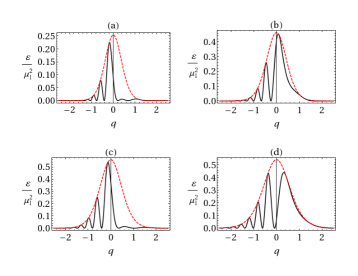
Figure 2: (Color online). Energy density [see Eq. (39)] for the 1D junction with $d_{x}=8$, $\mu_{H}=\mu_{C}=0$ at the fluxon velocity $v=0.398$ (a), $v=0.488$ (b), $v=0.552$ (c) and $v=0.676$ (d). The red dashed line depicts the $\mbox{sech}^{2}$ “envelope” term in Eq. (39).

As a result, for these values of $v$ the forward radiation can be insignificant, as can be observed from the area below the curve ${\cal E}(q)$ at $q>0$. In another case, the pair of minima that correspond to $n_{0}$ are significantly separated, and the maximum between them belongs to the set (41). It is again the first maximum at the positive axis, and it attains the value of ${\cal E}$ which is quite large comparing to the previous case, as can be seen in Figs. 2(b) and 2(d).

The dashed lines $6$ and $7$ in Fig. 3 show the dependence of the total emitted energy on the fluxon velocity (the solid lines correspond to the 2D case which will be discussed later). The values of $v$ which correspond to the minima of the $E(v)$ in line 6 in Fig. 3, have the minimal forward emission, and the respective spectral energy distributions are shown in Fig. 2(a), 2(c). The values of $v$ that are the maxima of $E(v)$ correspond to the maximal forward emission and the respective spectral distributions are given in Figs. 2(b) and 2(d). Thus, the maxima of the total energy coincide with the maximal forward emission while the minima of $E(v)$ correspond to the minimal forward emission. It should be noted that the minima [Eq. (40)] and maxima [Eq. (41)] of the energy density are distributed approximately equidistantly for the short-wavelength ($|q|\gg 1$) modes but with the different step for $q>0$ and $q<0$. In the limit $|v|\ll 1$ this step becomes approximately the same, it equals $2\pi v/d_{x}$. Consequently, in the limit $|v|\to 0$ one cannot expect sharply pronounced extrema of the $E(v)$ dependence, and this can be noticed from the inset.

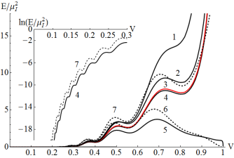
Figure 3: (Color online). Total emitted energy (normalized to $\mu_{I}^{2}$) as a function of the soliton velocity for the impurity with $d_{x}=8$, $d_{y}=8$ and $\mu_{H}=0$, $\mu_{C}=0.1$, $\mu_{C}/\mu_{I}=1$ (curve 1), $\mu_{H}=0$, $\mu_{C}=-0.05$, $\mu_{C}/\mu_{I}=0.5$ (curve 2), $\mu_{H}/\mu_{I}=0.01$, $\mu_{C}=0.05$, $\mu_{C}/\mu_{I}=0.5$ (curve 3, red), $\mu_{H}=0$, $\mu_{C}=0.05$, $\mu_{C}/\mu_{I}=0.5$ (curve 4), and $\mu_{H}=\mu_{C}=0$ (curve 5). The dashed lines 6 and 7 correspond to the same dependence but for the 1D problem [see Eq. (39) for the spectral energy density] with $d_{x}=8$ and $\mu_{H}=\mu_{C}=0$ (curve 6) and $\mu_{H}=0$, $\mu_{C}/\mu_{I}=0.5$, $\mu_{C}=0.05$ (curve 7). These dependencies are multiplied by a factor $10$ for the sake of convenience. The inset shows the details of the curves 4 and 7.

Finally, we remark that in the relativistic limit $v\to 1$ the total energy $E(v)\to 0$ if $\mu_{H}=\mu_{C}=0$ and $E(v)\to\infty$ if $\mu_{H,C}\neq 0$. The details of this limit will be discussed below together with the 2D case.

III.2.3 Total emitted energy in the 2D case

First of all, we discuss the dependence of the total emitted energy $E(v)$ on the impurity parameters $\mu_{I}$, $\mu_{H}$ and $\mu_{C}$. We remind the reader that $\mu_{I}$ is associated with the change of the critical current, while $\mu_{C}$ [see Eq. (7)] and $\mu_{H}$ [see Eq. (11)] appear due to the narrowing or distension of the insulating area. If $\mu_{H}=\mu_{C}=0$ the impurity corresponds only to the local change of the critical current without any changes in the insulating layer thickness. The total emitted energy for the different values of $\mu_{H}$ and $\mu_{C}$ is given in Fig. 3. We note the principal difference in the behavior of the $E(v)$ function in the limit $v\to 1$ if $\mu_{C,H}\neq 0$ compared to the case $\mu_{C}=\mu_{H}=0$. In the latter case $E(v)$ tends to zero while in the former case it diverges: $E(v)_{v\to 1}\to+\infty$. The same is observed in the 1D case (shown by the dashed lines). It is quite obvious from the lines 1 and 4 that for the larger values of $\mu_{C}$ the value of the emitted energy is larger. If one takes two opposite values of $\mu_{C}$, the case of a microresistor ($\mu_{C}<0$, line 2) yields slightly larger energy emission compared to the case of a microshort ($\mu_{C}>0$, line 4) due to the presence of the $(1+\mu_{C})^{-1}$ coefficient in the energy density (37). The effect of the spatial variation of the magnetic field, governed by the coefficient $\mu_{H}$ is negligible, as one can observe from the comparison of the lines 3 and 4. Therefore, we will assume $\mu_{H}=0$ further on throughout the paper.

The divergence at $v\to 1$ appears due to the presence of the divergent terms on the right-hand side of Eq. (21). These terms [see Eq. (22)] are proportional to $(1-v^{2})^{-1}$ and $(1-v^{2})^{-1/2}$. In the former term the function ${\bar{f}}_{I}$ contains both the parameters $\mu_{C}$ and $\mu_{H}$ and is always finite, thus the divergence appears only due to the divisor. In the latter term, in addition, there is a function $h_{H}$ which is non-zero only on the edges of the inhomogeneity, where it is proportional to the Dirac’s $\delta-$function. This term generates the sharp growth of radiation when the fluxon interacts with the edges of the impurity. In the 1D case it produces such growth only at the entrance ($x=-d_{x}/2$) and exit ($x=d_{x}/2$) points of the impurity.

We would like to mention that the divergence at $v\to 1$ seems to be non physical. First of all, the presence of the divergent term in Eq. (22) means that the first order of perturbation theory is not applicable any longer in this limit and should be amended somehow. Secondly, within the current model the dissipative effects have been neglected. If they are taken into account, the radiated energy will always be finite.

Other features of the $E(v)$ dependence such as the multiple extrema will be discussed below. At this point we only note that as $\mu_{C}$ decreases, the positions of the extrema do not shift significantly, but the absolute values of $E$ at the extrema decrease. This happens because the contribution to the emitted radiation due to the narrowing/expansion of the insulating layer, decreases. Depending on the value of $\mu_{C}$ some extrema can disappear due to the growth of $E(v)$ as $v\to 1$ (see line 1 in Fig. 3). The limit $v\to 0$ is given in the inset of Fig. 3. One can notice that the extrema of the total energy persist in this limit both in the 1D and 2D cases, although they can be spotted only on the logarithmic scale.

In Fig. 4 the total emitted energy is plotted for the fixed value of the impurity length $d_{x}=8$ while its width $d_{y}$ is varied. The 1D result for the same length is plotted with the dashed line as a reference. Naturally, the value of the emitted energy decreases as $d_{y}$ decreases. More interestingly, the extrema become less pronounced, and, finally no extrema are seen in curve 4 that corresponds to the case $d_{y}=2$. In the case $\mu_{H}=\mu_{C}=0$ we obtain the same picture: compare curve 5 of Fig. 3 ($d_{y}=8$), curve 5 of Fig. 4 ($d_{y}=6$), and curve 6 of Fig. 4 ($d_{y}=2$). The maxima become more shallow and gradually disappear. The following interpretation of the obtained results can be made. The shape of the energy density distribution is given in Fig. 5. The absolute minima of the energy density satisfy ${\cal E}(q_{x},q_{y})=0$ and these minimal values are attained at the following set on the $(q_{x},q_{y})$ plane:

$$q_{y}=\frac{2\pi n}{d_{y}}~{},~{}~{}n=\pm 1,\pm 2,\ldots~{}~{}\mbox{for any}~{}~{}q_{x},$$ (42)

$$(1-v^{2})q_{x}^{2}+q_{y}^{2}=\left(\frac{2\pi mv}{d_{x}}\right)^{2}-1+\frac{4\pi mv^{2}}{d_{x}}q_{x},$$ (43)

$$~{}~{}m=n_{0},n_{0}+1,\ldots~{},$$

where $n_{0}$ is given by Eq. (40). Thus, the minima are located on the set of parallel lines (42) as well as on the set of embedded ellipses given by Eq. (43). The ridges of the maximal ${\cal E}$ lie between the curves, defined by the roots of Eq. (42). For large $d_{y}$ these ridges are strongly localized in the $q_{y}$ direction [see Figs. 5(a) and 5(b)], while the decreasing of $d_{y}$ makes them concentric and crescent-like as shown in Figs. 5(c) and 5(d).

For the large values of $d_{y}$ the problem can be treated as an almost 1D, so that most of the emitted radiation travels in the $x$ direction while the $y$- component of the radiation remains insignificant.

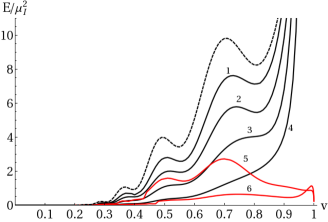
Figure 4: (Color online) Total emitted energy (normalized to $\mu_{I}^{2}$) as a function of the fluxon velocity for $\mu_{H}=0$, $\mu_{C}/\mu_{I}=0.5$, $\mu_{C}=0.05$, $d_{x}=8$ and $d_{y}=8$ (curve 1), $d_{y}=6$ (curve 2), $d_{y}=4$ (curve 3), and $d_{y}=2$ (curve 4). The case $\mu_{H}=\mu_{C}=0$ is represented by the red curves 5 ($d_{y}=6$) and 6 ($d_{y}=2$). The dashed line corresponds to the respective 1D problem with $d_{x}=8$ (for the sake of convenience it is multiplied by a factor of 10).

This can be clearly observed in Figs. 5(a) and 5(b) where the spectral density ${\cal E}(q_{x},q_{y})$ (37) is plotted for the values of velocity close to the minimum [panel a] and maximum [panel b] of the curve $1$ in Fig. 4. Since the decay of the function $[\sin(q_{y}d_{y}/2)/q_{y}]^{2}$ with the growth of $q_{y}$ is quite fast for the large values of $d_{y}$, the energy density function remains strongly localized along the $q_{x}$ axis in the neighbourhood of the $q_{y}=0$ line. Its behaviour along the $q_{x}$ axis is reminiscent of the respective 1D problem, see Eq. (39) and Fig. 2. Indeed, the minimum of the total emitted energy corresponds to the minimal forward emission. It can be easily observed in Fig. 5(a) that the global maximum is placed on the $q_{x}$ axis at $q_{x}<0$ while the first local maximum at $q_{x}>0$ is rather small. In Fig. 5(b) it can be seen that the global maximum is placed on the positive half-axis of the $q_{x}$ axis, and this happens at $v=0.73$ which is quite close to the maximum of the $E(v)$ function (curve $1$) in Fig. 4.

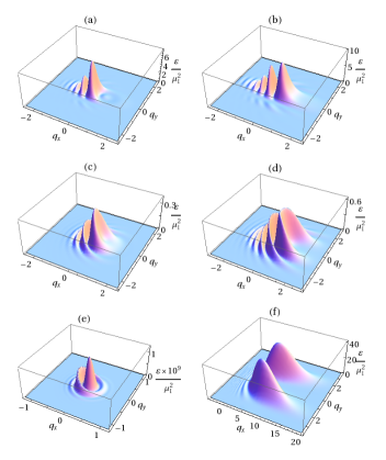
Figure 5: (Color online). Emitted energy density ${\cal E}$ for the data in Fig. 4, curve $1$ at $v=0.55$ (a) and $v=0.73$ (b); curve $6$ at $v=0.5$ (c), $v=0.75$ (d), $v=0.1$ (e) and $v=0.99$ (f).

The further decreasing of $d_{y}$ smears out maxima in the $E(v)$ dependence (compare the curves $1$-$4$ in Fig. 5) up to the point when only one local maximum can be spotted. The scattering problem cannot be considered as a quasi-1D any more. The radiation distribution becomes rather different as shown in Figs. 5(c) and 5(d). The maxima of ${\cal E}(q_{x},q_{y})$ still lie on the $q_{x}$ axis, but the curves (43) that define the minimal values become distinctly arc shaped. The $y$- component of the radiation becomes more delocalized and the analogy with the 1D picture breaks down.

It is interesting to note how the shape of the energy density function varies in the extreme limits of the velocity value: $v\to 0$ and $v\to 1$. In the small velocity limit $|v|\ll 1$ the ellipses Eq. (43) that correspond to the minima of ${\cal E}$ are almost circles and the density function is close to being radially symmetric, see Fig. 5(e). The increasing of $v$ makes the ellipses Eq. (43) more elongated in the $x$ direction, as has been demonstrated previously [see Figs. 5(a)-(d)]. An interesting situation emerges in the opposite limit, namely if $1-|v|\ll 1$. The global maximum that was positioned on the $q_{x}$ axis splits up into two maxima that are now located off the $q_{x}$ axis symmetrically with respect to each other, as shown in Fig. 5(f). Physically this means the following. The slow fluxon “feels” the impurity as a wall and the emergent radiation moves mostly along the fluxon propagation direction. The fast (relativistic) fluxon interacts with the impurity in such a way that the impurity acts like a groin (a wave- breaker) and the emitted radiation is split by the impurity into two halves that have both $x$ and $y$ components. A the same time the $x$ component of the radiation becomes insignificant.

The number of local extrema of $E(v)$ depends on the impurity length $d_{x}$. This is easily demonstrated by Fig. 6, where the number of the maxima decreases with the decreasing of $d_{x}$. This result is similar to the same situation in the 1D model Kivshar et al. (1988).

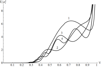
Figure 6: Total emitted energy (normalized to $\mu_{I}^{2}$) as a function of the fluxon velocity for $\mu_{H}=0$, $\mu_{C}/\mu_{I}=0.2$, $\mu_{C}=0.02$, $d_{y}=8$ and $d_{x}=2$ (curve 1), $d_{x}=4$ (curve 2), $d_{x}=6$ (curve 3), and $d_{x}=10$ (curve 4).

III.2.4 Limiting cases

It is of interest to check the limiting cases when in one of the directions ($x$ or $y$) the impurity becomes infinitely narrow. In the first case the limit $d_{x}\to 0$, while $\mu_{*}=\mu_{I}d_{x}$ remains constant, corresponds to the situation when the impurity becomes infinitely thin in the $x$ direction. In Eqs. (34) and (35) the difference of the $\theta$-functions that form the first factor in the functions $f_{I,H,C}(x,y)$ (34) becomes the Dirac $\delta$ function while $h_{H}\equiv 0$. This case with $\mu_{C}=\mu_{H}=0$ has been studied previously Starodub and Zolotaryuk (2013). Yet another interesting limit can be considered if $d_{y}\to 0$, $\mu_{*}=\mu_{I}d_{y}$. In other words, the impurity remains elongated in the $x$ direction, but becomes infinitely thin in the $y$ direction. The spectral density of the emitted plasmons in the cases mentioned above reads

$$\frac{{\cal E}(q_{x},q_{y})}{\mu_{*}^{2}}\to\left\{\begin{array}[]{ccc}\displaystyle\hfil&&\displaystyle\frac{\sin^{2}\left(\frac{q_{y}d_{y}}{2}\right)}{2v^{6}q_{y}^{2}}\frac{\left\{{1-v^{2}-{\mu_{H}\over\mu_{I}}+v^{2}{\mu_{C}\over\mu_{I}}\over{1+\mu_{C}}}\left[(\omega-q_{x}v)^{2}+q_{y}^{2}v^{2}\right]+2{\mu_{H}\over\mu_{I}}(\omega-vq_{x})^{2}\right\}^{2}}{(\omega-q_{x}v)^{2}+(v^{2}-1)q_{y}^{2}}\times\\ &&~{}\times\text{sech}^{2}\left(\frac{\pi\omega\sqrt{1-v^{2}}}{2v}\right)~{},~{}~{}\textrm{if}~{}d_{x}\to 0,\\ &&\displaystyle\frac{1}{2v^{4}}\left[\frac{\sin[d_{x}(\omega-q_{x}v)/2v]}{\omega-q_{x}v}\right]^{2}\displaystyle\frac{\left\{{1-v^{2}-{\mu_{H}\over\mu_{I}}+v^{2}{\mu_{C}\over\mu_{I}}\over{1+\mu_{C}}}\left[(\omega-q_{x}v)^{2}+q_{y}^{2}v^{2}\right]+2{\mu_{H}\over\mu_{I}}(\omega-vq_{x})^{2}\right\}^{2}}{(\omega-q_{x}v)^{2}+(v^{2}-1)q_{y}^{2}}\times\\ &&~{}\times\text{sech}^{2}\left(\frac{\pi\omega\sqrt{1-v^{2}}}{2v}\right)\,,~{}~{}~{}\textrm{if}~{}d_{y}\to 0~{}.\end{array}\right.$$ (48)

In these limits the modulation in $q$- space, caused by the interference, disappears along the $q_{x}$ direction in the first formula because the impurity length becomes infinitely small. For the same reason there is no interference along the $q_{y}$ component when $d_{y}\to 0$ in the second formula of Eq. (LABEL:29d). When any of these limits are approached, the multiple maxima of the $E(v)$ dependence disappear leaving only one local maximum. The limit of the point [$f_{I}(x,y)=\mu_{I}\delta(x)\delta(y)$] impurity Malomed (1991) can be achieved easily from the stripe impurity by taking in Eqs. (48) the limits $\mu_{C,H}\to 0$ and $d_{x}\to 0$ or $d_{y}\to 0$ where appropriate. When the impurity shrinks into a point the local change of the insulating layer thickness is ignored; thus $\mu_{C}=\mu_{H}=0$. The obtained formula coincides with the previous result Malomed (1991).

III.3 Rhombic impurity

Now we consider the rhombus(diamond)-shaped impurity with $d_{x}$ and $d_{y}$ being its length and width respectively:

$$\Omega:~{}~{}|x|\leq d_{x}/2~{}\bigcap~{}|y|\leq g(x)=d_{y}(1/2-|x|/d_{x})~{}.$$ (49)

The tip of the rhombus is perpendicular to the fluxon line. Then

$$h_{H}(x,y) = \mu_{H}\left\{\left[\delta(x+d_{x}/2)-\delta(x-d_{x}/2)\right]\times\right.$$ (50)

$$\times \left.\left[\theta(y+g(x))-\theta(y-g(x))\right]\right.+$$

$$+ \left.\left[\theta(x+d_{x}/2)-\theta(x-d_{x}/2)\right]\right.\times$$

$$\times \left.\left\{\delta[y-g(x)]+\delta[y+g(x)]\right\}g^{\prime}(x)\right\},$$

$$g^{\prime}(x) = -\frac{d_{y}}{d_{x}}\mbox{sign}(x)=-\frac{d_{y}}{d_{x}}\mbox{sign}(\xi+v\tau)~{}.$$ (51)

Substituting the formulas (50) and (51) into Eqs. (28) and (29) we obtain the radiation function in the moving frame:

$$B(q_{\xi},q_{y}) = i\frac{2\sqrt{2\pi}\mu_{I}}{q_{y}^{2}\sqrt{1+q_{\xi}^{2}}(1-v^{2})^{1/2}v^{3}}{d_{x}\over d_{y}}\left\{\left(1-v^{2}-{\mu_{H}\over\mu_{I}}+v^{2}{\mu_{C}\over\mu_{I}}\right){[{\bar{\omega}}^{2}-(1+q_{\xi}^{2})v^{2}]\over{1+\mu_{C}}}+2{\mu_{H}\over\mu_{I}}(1-v^{2}){\bar{\omega}}^{2}\right\}\times$$ (52)

$$\times \frac{\cos\left(\frac{q_{y}d_{y}}{2}\right)-\cos\left(\frac{\bar{\omega}\sqrt{1-v^{2}}}{2v}d_{x}\right)}{({d_{x}\over d_{y}}{\bar{\omega}})^{2}\frac{1-v^{2}}{q_{y}^{2}v^{2}}-1}\mbox{sech}\left[{\frac{\pi}{2v}(q_{\xi}v+{\bar{\omega}})}\right]~{},$$

where the dispersion law $\bar{\omega}=\bar{\omega}(q_{\xi},q_{y})$ in the moving frame is given by Eq. (26). The transition to the laboratory frame is performed in the standard way, and- as a result, the spectral energy density in the laboratory frame is expressed by the following formula:

$${\cal E}(q_{x},q_{y}) = \frac{2\mu_{I}^{2}}{v^{2}}\left(\frac{d_{x}}{d_{y}}\right)^{2}\left\{\frac{\cos(q_{y}d_{y}/2)-\cos[d_{x}(\omega-q_{x}v)/2v]}{\left(\frac{d_{x}}{d_{y}}\right)^{2}(\omega-q_{x}v)^{2}-v^{2}q_{y}^{2}}\mbox{sech}\left(\frac{\pi\omega}{2v}\sqrt{1-v^{2}}\right)\right\}^{2}\times$$ (53)

$$\times \frac{\left[{1-v^{2}-{\mu_{H}\over\mu_{I}}+v^{2}{\mu_{C}\over\mu_{I}}\over(1+\mu_{C})}\left((\omega-q_{x}v)^{2}+q_{y}^{2}v^{2}\right)+2{\mu_{H}\over\mu_{I}}(\omega-vq_{x})^{2}\right]^{2}}{(\omega-q_{x}v)^{2}+(v^{2}-1)q_{y}^{2}}~{},$$

where the dispersion law $\omega=\omega(q_{x},q_{y})$ in the laboratory frame is given by Eq. (38). It may seem that this dependence has a singularity where the equation $\left(\frac{d_{x}}{d_{y}}\right)^{2}(\omega-q_{x}v)^{2}=v^{2}q_{y}^{2}$ is satisfied. However, with the help of the trigonometric formula $\cos a-\cos b=2\sin[(a+b)/2]\sin[(b-a)/2]$ it is straightforward to show that the respective divergences cancel out.

The total emitted energy as a function of the fluxon velocity $v$ is shown in Figs. 7-9. The first figure (Fig. 7) focuses on the situation when the ratio $d_{y}/d_{x}$ is fixed while the area covered by the impurity is varied. The main figure correspond to the impurity with its narrow edge pointing towards the fluxon direction ($d_{x}/d_{y}=4$). The inset (a) describes the opposite situation: $d_{y}/d_{x}=4$. In general, the dependence $E(v)$ grows with $v$ in the limit $v\ll 1$ and diverges at $v\to 1$ due to the presence of the $\mu_{C}$ and $\mu_{H}$ terms [otherwise, if $\mu_{C}=\mu_{H}=0$, we have $E(v)_{v\to 1}\to 0$]. This behavior is quite similar to the case of the rectangular impurity studied in III.2.

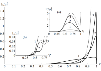
Figure 7: Total emitted energy (normalized to $\mu_{I}^{2}$) as a function of the fluxon velocity for the rhombic impurity with the fixed ratio $d_{x}/d_{y}=4$. The solid lines correspond to $\mu_{C}=\mu_{H}=0$, $d_{x}=4$ (curve 1), $d_{x}=8$ (curve 2) and $d_{x}=12$ (curve 3). The dashed line corresponds to $d_{x}=12$ and $\mu_{C}=0.01$ and $\mu_{C}/\mu_{I}=0.1$, $\mu_{C}=0.01$, $\mu_{H}=0$. The inset (a) corresponds to the case $d_{x}/d_{y}=1/4$, $\mu_{C}=\mu_{H}=0$ $d_{x}=1$ (curve 1), $d_{x}=2$ (curve 2) and $d_{x}=3$ (curve 3) and $\mu_{C}/\mu_{I}=0.1$, $\mu_{H}=0$, $d_{x}=3$ (dashed curve). The inset (b) shows the details of the main figure.

First we consider the rhombus, elongated towards the fluxon propagation direction (main part of Fig. 7). We observe that in the case $\mu_{C}=\mu_{H}=0$ there is one well- established maximum of the $E(v)$ dependence which is positioned very close to the value $v=1$. As the impurity area is increased, the peak of the energy dependence sharpens, while the position of the maximum shifts towards the point $v=1$. If $\mu_{C}\neq 0$ the main maximum disappears due to the unbounded growth of the energy dependence. There are other maxima of the $E(v)$ dependence, however they are very weak and can be noticed only if the respective region is zoomed [see the inset (b)]. When the impurity area decreases, some of these maxima disappear [compare the curves 3 and 2 in the the inset (b)].

Inset (a) of Fig. 7 corresponds to the situation when the impurity is elongated in the $y$- direction with the ratio $d_{x}/d_{y}=1/4$ being fixed. In this case there is only one local maximum that decreases while the adjacent local minimum becomes more shallow as the area $d_{x}d_{y}/2$ decreases. This case is qualitatively close to the limit of the strip impurity Starodub and Zolotaryuk (2013) but the limit (48) is not restored mathematically.

It is possible to consider the limiting cases of the infinitely narrow stripes: $d_{x}\to 0$ and $d_{y}\to 0$. If the impurity amplitude is redefined as $\mu_{*}=\mu_{I}d_{x}$ (or $\mu_{*}=\mu_{I}d_{y}$), the spectral density in these limits reads

$$\frac{{\cal E}(q_{x},q_{y})}{\mu_{*}^{2}}\to\left\{\begin{array}[]{ccc}\displaystyle\hfil&&\displaystyle 8\frac{\sin^{4}\left(\frac{q_{y}d_{y}}{4}\right)}{v^{6}d_{y}^{2}q_{y}^{4}}\frac{\left\{{1-v^{2}-{\mu_{H}\over\mu_{I}}+v^{2}{\mu_{C}\over\mu_{I}}\over 1+\mu_{C}}\left[(\omega-q_{x}v)^{2}+q_{y}^{2}v^{2}\right]+2{\mu_{H}\over\mu_{I}}(\omega-vq_{x})^{2}\right\}^{2}}{(\omega-q_{x}v)^{2}+(v^{2}-1)q_{y}^{2}}\times\\ &&~{}\times~{}\text{sech}^{2}\left(\frac{\pi\omega\sqrt{1-v^{2}}}{2v}\right)~{},~{}~{}\textrm{if}~{}d_{x}\to 0,\\ &&\displaystyle{{8}\over{d_{x}^{2}v^{2}}}\left\{\frac{\sin[d_{x}(\omega-q_{x}v)/4v]}{\omega-q_{x}v}\right\}^{4}\frac{\left\{{1-v^{2}-{\mu_{H}\over\mu_{I}}+v^{2}{\mu_{C}\over\mu_{I}}\over 1+\mu_{C}}\left[(\omega-q_{x}v)^{2}+q_{y}^{2}v^{2}\right]+2{\mu_{H}\over\mu_{I}}(\omega-vq_{x})^{2}\right\}^{2}}{(\omega-q_{x}v)^{2}+(v^{2}-1)q_{y}^{2}}\times\\ &&~{}\times\text{sech}^{2}\left(\frac{\pi\omega\sqrt{1-v^{2}}}{2v}\right)\,~{}~{}~{}\textrm{if}~{}d_{y}\to 0~{}.\end{array}\right.$$ (58)

These limiting values of ${\cal E}$ are very similar to the analogous limits for the rectangular impurity (48). The only principal difference is the interference terms that are responsible for the oscillations in the $q_{x}$ or $q_{y}$ direction come with the power $4$ and not $2$ as in Eq. (48).

Next we focus on the situation when the impurity width $d_{y}$ is fixed and its length $d_{x}$ is varied. In Fig. 8(a) the dependence of the local maximum value (defined within the interval $0\leq v<1$) of the emitted energy as a function of the rhombus angle $\arctan(d_{y}/d_{x})$ is plotted. If $\mu_{C}=\mu_{H}=0$ the $\max_{v\in[0,1[}E(v)$ dependence on the rhombus angle is a decaying function almost everywhere in the interval $[0,\pi/2]$. In the limit $d_{x}\to\infty$ the maximum of $E(v)$ grows as the amount of the emitted energy increases. Only in the neighborhood of the angle $\pi/3$ there is a weakly pronounced local maximum. If $\mu_{C}\neq 0$ such a dependence cannot be defined for the whole interval $[0,\pi/2]$ and it starts from some critical value of the angle (see the dependencies, marked by squares and inverted triangles) and continues till the value $\pi/2$.

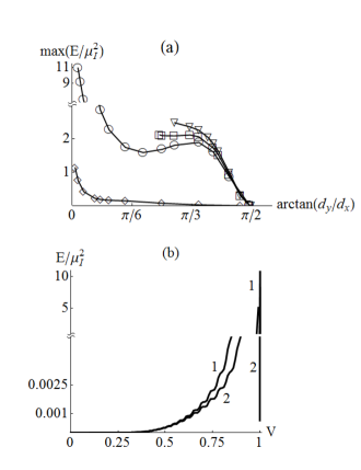
Figure 8: (a) The value of the local maximum $\max_{v\in[0,1[}E(v)$ of the emitted energy (normalized to $\mu_{I}^{2}$) as a function of the angle $\arctan(d_{y}/d_{x})$ for the parameters $d_{y}=5$, $\mu_{C}=0.01$, $\mu_{C}/\mu_{I}=0.1$ ($\nabla$), $\mu_{C}=0.005$, $\mu_{C}/\mu_{I}=0.05$ ($\Box$), $\mu_{C}=0$ ($\circ$) and $d_{y}=1$, $\mu_{C}=0$ ($\diamond$). The solid line is used as a guide for an eye.
(b) Emitted energy dependence (normalized to $\mu_{I}^{2}$) as a function of the fluxon velocity for $d_{x}=100$, $d_{y}=5$, $\mu_{C}=0.01$, $\mu_{C}/\mu_{I}=0.1$ (curve 1) and $\mu_{C}=0$ (curve 2). $\mu_{H}=0$ everywhere.

Below this critical angle there is no local maximum of $E(v)$ because it becomes strictly monotonic. If $d_{y}$ is decreased, the dependence becomes a strictly decaying function (shown by the circles in Fig. 8) that cover the whole interval $[0,\pi/2]$ even if $\mu_{C}\neq 0$. In Fig. 8(b) the $E(v)$ dependence is demonstrated in the limit of the extremely narrow rhombic impurity. If $\mu_{C}>0$ there is no maximum and the $E(v)$ function is a monotonically increasing function. If $\mu_{C}=0$ there is a sharp maximum very close to $v=1$ and everywhere else the function behaves almost identically to the case $\mu_{C}>0$. One can notice a fine structure of multiple inflection points. These points are the remnants of the local maxima that are clearly seen in the inset (b) of Fig. 7. The number of these inflection points increases as the length of the rhombus $d_{x}$ increases. Here we observe a weak link with the case of the rectangular impurity, studied in III.2. In that case we reported the increasing of the number of maxima of $E(v)$ when $d_{x}$ increased. For the rhombus we see the maxima degenerate into the inflection points. The limit $d_{x}\to\infty$ means that the impurity acts as an extremely narrow groin that does not cause much radiation due to its narrowness for small and intermediate velocities. Significant growth of the emitted radiation can be spotted only in the relativistic regime ($1-v^{2}\ll 1$). It is important to remark that there is no clear 1D limit for the rhombic impurity, while such a limit can be achieved for the rectangular impurity by setting $d_{y}\to\infty$.

In the limits $d_{x}\to 0$ the radiated energy decreases significantly as one obtains infinitely thin impurity in the $x$ direction. When this limit is approached the local maximum of the $E(v)$ dependence becomes less and less pronounced. The energy density is proportional to $d_{x}^{2}$; thus, it is not surprising that the total energy tends to zero in this limit. The renormalization of the impurity amplitude $\mu_{*}=\mu_{I}d_{x}$ and $d_{x}\to 0$ will lead the first formula of Eq. (LABEL:31).

If the rhombus becomes a square ($d_{x}=d_{y}$) the local maximum of the radiation becomes more pronounced if the area of the impurity increases, as shown in Fig. 9. Also, the decreasing of the impurity area makes the local maximum less pronounced. The main maximum is dominant, although there exist secondary local maxima, to the left from the main maximum, although they are very small. The position of the main maximum shifts to the left as the impurity size is decreased; however this shift is insignificant even if the area $d_{x}d_{y}/2$ is decreased by the order of magnitude (compare the curves 4 and 6 in Fig. 9).

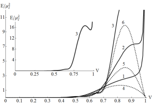
Figure 9: Total emitted energy (normalized to $\mu_{I}^{2}$) as a function of the fluxon velocity for the square rhombic ($d_{x}=d_{y}$) impurity at $\mu_{H}=0$, $\mu_{C}=0.01$, $\mu_{C}/\mu_{I}=0.1$, $d_{x}=d_{y}=5$ (curve 1), $d_{x}=d_{y}=10$ (curve 2), $d_{x}=d_{y}=20$ (curve 3). The dashed lines corresponds to the case $\mu_{H}=\mu_{C}=0$ and $d_{x}=d_{y}=5$ (curve 4), $d_{x}=d_{y}=10$ (curve 5), $d_{x}=d_{y}=20$ (curve 6). The inset gives the details of curve 3 on the larger scale.

Reducing the size of the impurity in both directions ($d_{x},d_{y}\to 0$, and $\mu_{C,H}\to 0$) brings the spectral energy density function (53) to the already known limit of the point-like impurityMalomed (1991). The same limit can be obtained from any of the Eqs. (LABEL:31) by setting $d_{y}\to 0$, $\mu_{C,H}\to 0$ in the first equation or $d_{x}\to 0$, $\mu_{C,H}\to 0$ in the second equation. The impurity amplitude should be redefined as $\mu_{*}=\mu_{I}d_{y}$ or $\mu_{*}=\mu_{I}d_{x}$, respectively.

The energy density profiles ${\cal E}(q_{x},q_{y})$ that correspond to the rhombic impurity are presented in Fig. 10. As a particular example, we consider an impurity that corresponds to the curve $3$ from Fig. 7, i.e., for $d_{x}=12$, $d_{y}=3$. This energy density distribution bears many qualitative similarities with the energy density function for the rectangular impurity shown in Fig. 5.

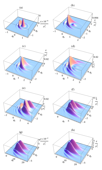
Figure 10: (Color online). Emitted energy density ${\cal E}$ for the rhombic impurity with $d_{x}=12$, $d_{y}=3$, $\mu_{C}=\mu_{H}=0$ (curve 3 in Fig. 7) at $v=0.2$ (a), $v=0.47$ (b), $v=0.63$ (c), $v=0.75$ (d), $v=0.85$ (e), $v=0.95$ (f), and $v=0.993$ (g). The panel (h) corresponds to $v=0.993$ and $\mu_{C}=0.01$, $\mu_{C}/\mu_{I}=0.1$.

The global minima of the energy density satisfy the condition ${\cal E}(q_{x},q_{y})=0$ and are given by the set of equations

$$d_{x}\left(\frac{\sqrt{1+q_{x}^{2}+q_{y}^{2}}}{v}-q_{x}\right)\pm q_{y}d_{y}=4\pi n_{\mp}~{}.$$ (59)

This set of equations describes the sequence of pairs of ellipses that are numbered by the integers $n_{\pm}$,

$$n_{\mp}=n_{0},n_{0}+1,\ldots,~{}n_{0}=\left\lceil\frac{d_{x}}{4\pi}\sqrt{\frac{1}{v^{2}}-\frac{d_{x}^{2}+d_{y}^{2}}{d_{x}^{2}}}\right\rceil~{}.$$ (60)

if

$$|v|<\frac{d_{x}}{\sqrt{d_{x}^{2}+d_{y}^{2}}}~{}.$$ (61)

Otherwise, the Eqs. (59) yield the set of hyperbolas that are numbered with $n_{\pm}=\pm 1,\pm 2,\ldots$. The two curves (ellipses or hyperbolas) given by Eq. (59) that correspond to the opposite signs but with $n_{+}=n_{-}$ are mapped into each other with the mirror symmetry with respect to the $q_{x}$ axis. If we consider the set of curves with the same sign, say $+$, they are embedded into each other and they expand with the growth of the index $n_{+}$. Between these curves lie the ridges of the ${\cal E}(q_{x},q_{y})$ function, and the local maxima of the energy density lie on these ridges.

The signatures of these curves can be spotted in all panels of Fig. 10. For small and intermediate values of the fluxon velocity the emitted radiation is localized predominantly in one peak in the $q-$space, as shown in Figs. 10(a-d). This peak lies on the $q_{x}$ axis; thus, most of the radiation does not propagate in the perpendicular direction. In the panel (a) one can observe the distribution for the rather small value of the fluxon velocity ($v=0.2$) and this distribution is close to being radial. At such small velocities the pair of ellipses (59) with $n_{-}=n_{+}$ are very close to being circles and almost coincide with each other. For larger values of $v$ these pairs start to separate, as illustrated in Figs. 10(b-e). The panel (b) corresponds to the local minimum of $E(v)$ (curve $3$ of Fig. 7) at $v=0.47$ while the panel (c) corresponds to the local maximum at $v=0.63$. The structure of both these functions is similar and the only difference is that the maximal peak in panel (c) lies in the area of backward radiation ($q_{x}\approx-0.25$), while in panel (c) the main peak lies on the positive half of the $q_{x}$ axis at $q_{x}\approx 0.3$. Thus, for the intermediate velocities the situation is similar to the case of rectangular impurity, where the minimum of $E(v)$ corresponded to the minimal forward radiation. Panel (d) corresponds to the next local minimum of the $E(v)$ curve at $v=0.75$, and here one observes the increasing of the share of the perpendicular radiation in the total radiated energy. The further increasing of $v$ leads to the appearance of the pair of equivalent local maxima off the $q_{y}=0$ axis [see panel (e)]. These maxima become global as $v$ approaches the value $v=1$ [see panels (f) and (g)]. Thus, we observe the increasing of the perpendicular radiation that reaches its climax in the relativistic limit $v\to 1$. Panel (f) corresponds to the maximum of the $E(v)$ function (curve $3$ of Fig. 7) at $v=0.993$. According to Eq. (61) the minima of the energy density lie on the hyperbolas and the maxima lie between these hyperbolas and off the $q_{x}$ axis. They appear to be strongly localized in the $q_{y}$ direction while their localization in the $q_{x}$ is significantly weaker. In this limit the interaction time with the tip of the rhombus is too small to generate significant longitudinal radiation, and the shape of the obstacle breaks the incident fluxon as a groin and generates predominantly transverse radiation.

Finally, we mention the dependence of the emitted energy on the parameter $\mu_{C}$. Panel (h) corresponds to the same parameters of the model as in panel (g) but with $\mu_{C}>0$. Comparing panels (g) and (h) we see that the structure of these functions is very similar while the absolute values of ${\cal E}$ are significantly smaller in the $\mu_{C}=0$ case. If $\mu_{C}=0$, but for the same value of the fluxon velocity, the values of the maxima actually decrease with $v$. Thus, the total emitted energy tends to zero, in the same way as shown by the dashed lines in Fig. 9. This has been confirmed for the values of $v$ even closer to unity as well as for the different values of $d_{x,y}$. The qualitative behavior of $E(v)$ in the limit $|v|\to 1$ appears to be the same both for the rectangular and rhombic impurities.

IV Discussion and conclusion

The radiation emitted as a result of the fluxon interaction with the impurity of a general geometrical shape in the large two-dimensional Josephson junction has been studied. The emitted energy distribution in the $q-$space has been computed as well as the total emitted energy. This energy distribution can always be represented as a triple integral. In principle, any geometrical shape can be taken into consideration; however, the explicit integration is not always possible, but if the inhomogeneity area can be represented by the piecewise-linear functions, this integration can be done. In this article the rectangular and rhombic impurities have been studied.

The main result of this work has been formulated in the dependence $E(v)$ of the total emitted energy as a function of the incident fluxon velocity. It appears that this dependence has local maxima that depend strongly on the geometric properties of the impurity. These local maxima do not exist if the impurity is treated as a pointMalomed (1991). Controlling the shape of the impurity one can remove the extrema or make them more pronounced. The limit of the 1D problem with the finite-size Kivshar et al. (1988) inhomogeneity can be restored.

First of all we would like to mention the differences between the 1D and 2D cases. The 1D case appears to be the limit of the 2D rectangular impurity case when $d_{y}\to\infty$. While moving away from the 1D limit by decreasing $d_{y}$ we observe gradual lowering and disappearance of the extrema of the $E(v)$ dependence. Next, the 2D model allows to take into account the impurity shapes that are different from the rectangle. For the rhombic impurity we have demonstrated that the emitted energy dependence on the fluxon velocity is rather different from the rectangular case and does not possess the 1D limit. In principle, other geometrical impurity shapes can be studied, including the asymmetric ones.

In this article the junction thickness change due to the homogeneity is taken into account. Its role is measured by the parameters $\mu_{H}$ and $\mu_{C}$ [see Eqs. (3) and (11)]. The parameter $\mu_{C}$ is responsible for the capacitance change and plays the dominant role. In some papers Balents and Simon (1995) these parameters are ignored (especially they are always ignored if the point impurities are considered), and, in general, are considered to be weak Kivshar et al. (1988). However, the junction thickness change influences significantly the asymptotic behavior of the total emitted energy in the “relativistic” (i.e., $v\to 1$) limit of the fluxon velocity. If the thickness change is ignored, the total emitted energy goes to zero, while it exhibits unbounded growth if the thickness change is taken into account. This is true for the both 1D and 2D junctions. The emitted energy has been computed under the assumption that it is a small perturbation on the fluxon background. Consideration of the higher order corrections may block the infinite radiation growth. Also, the dissipative effects, which have been ignored in this work, should contribute to the decreasing of the emitted energy.

Although the real large-area Josephson junctions have finite dimensions, in this article the infinitely-sized junction has been considered. This approximation is sufficient if the physical dimensions of the LJJ exceed by the order of magnitude the Josephson penetration depth and, consequently, the fluxon length in the $x$ direction. The boundary conditions are also important, however Lomdahl et al. (1985); Eilbeck et al. (1985), if the junction width is large enough (exceeds the Josephson length at least by the order of magnitude) the fluxon distortion from the linear shape is insignificant. In any case, before focusing on the more concrete setup an idealized, but more easily solvable model should be studied.

Finally, we discuss the possible application of the obtained results. Recently, a number of papers have focused on the different application of the fluxon dynamics in the 2D LJJ, such as fluxon splitting on the T-shaped junctions Gulevich and Kusmartsev (2006), excitation of the different modes that move along the fluxon front Gulevich et al. (2008, 2009), and the fluxon logic gates Nacak and Kusmartsev (2010) where the interaction with the spatial inhomogeneity takes place. If the incident fluxon velocity is large enough, the emitted radiation becomes sufficient and it should influence the fluxon motion. In particular, the non-monotonicity of the $E(v)$ dependence may produce the hysteresis-like branches Kivshar et al. (1988) on the current-voltage characteristics (IVCs) of the LJJ. Studies of these IVCs for the different shapes of the inhomogeneity in the genuinely 2D case are in progress and will be published elsewhere.

References

- Barone and Paterno (1982) A. Barone and G. Paterno, Physics and Applications of the Josephson Effect (Wiley, New York, 1982).
- (2) K. K. Likharev, Dynamics of Josephson Junctions and Circuits (Gordon and Breach, New York, 1986).
- McLaughlin and Scott (1978) D. W. McLaughlin and A. C. Scott, Phys. Rev. A 18, 1652 (1978).
- Gal’pern and Filippov (1984) Y. S. Gal’pern and A. T. Filippov, Sov. Phys. JETP 86, 1527 (1984).
- Aslamazov and Gurovich (1984) L. G. Aslamazov and E. V. Gurovich, JETP Lett. 40, 746 (1984).
- Fehrenbacher et al. (1992) R. Fehrenbacher, V. B. Geshkenbein, and G. Blatter, Phys. Rev. B 45, 5450 (1992).
- Balents and Simon (1995) L. Balents and S. H. Simon, Phys. Rev. B 51, 6515 (1995).
- Fistul and Giuliani (1998) M. V. Fistul and G. F. Giuliani, Phys. Rev. B 58, 9348 (1998).
- Mkrtchyan and Shmidt (1979) G. Mkrtchyan and V. V. Shmidt, Solit State Commun. 30, 791 (1979).
- Kivshar et al. (1988) Y. S. Kivshar, B. A. Malomed, and A. A. Nepomnyashchy, JETP 94, 356 (1988).
- Malomed et al. (1988) B. A. Malomed, I. L. Serpuchenko, M. I. Tribelsky, and A. V. Ustinov, JETP Lett. 47, 591 (1988).
- Malomed and Ustinov (1990) B. A. Malomed and A. V. Ustinov, J. Appl. Phys. 67, 3791 (1990).
- Kivshar and Chubykalo (1991) Y. S. Kivshar and O. A. Chubykalo, Phys. Rev. B 43, 5419 (1991).
- Kivshar et al. (1988) Y. S. Kivshar, A. M. Kosevich, and O. A. Chubykalo, Phys. Lett. A 129, 449 (1988).
- Kivshar et al. (1987) Y. S. Kivshar, A. M. Kosevich, and O. A. Chubykalo, Fiz. Nizk. Temp 13, 800 (1987).
- Lomdahl et al. (1985) P. S. Lomdahl, O. H. Olsen, J. C. Eilbeck, and M. R. Samuelsen, J. Appl. Phys. 57, 997 (1985).
- Lachenmann et al. (1993) S. G. Lachenmann, G. Filatrella, T. Doderer, J. C. Fernandez, and R. P. Huebener, Phys. Rev. B 48, 16623 (1993).
- Starodub and Zolotaryuk (2012) I. O. Starodub and Y. Zolotaryuk, Phys. Lett. A 376, 3101 (2012).
- Gulevich et al. (2009) D. R. Gulevich, F. V. Kusmartsev, S. Savel’ev, V. A. Yampol’skii, and F. Nori, Phys. Rev. B 80, 094509(13) (2009).
- Nacak and Kusmartsev (2010) H. Nacak and F. Kusmartsev, Physica C 470, 827 (2010).
- Malomed (1991) B. A. Malomed, Physica D 52, 157 (1991).
- Kivshar and Malomed (1988) Y. S. Kivshar and B. A. Malomed, Phys. Lett. A 129, 443 (1988).
- Rubinstein (1970) J. Rubinstein, J. Math. Phys. 11, 258 (1970).
- Salerno et al. (1984) M. Salerno, E. Joergensen, and M. Samuelsen, Phys. Rev. B 30, 2635 (1984).
- Graham et al. (1994) R. L. Graham, D. E. Knuth, and O. Patashnik, Concrete Mathematics (Addison-Wesley, Reading Ma., 1994).
- Starodub and Zolotaryuk (2013) I. O. Starodub and Y. Zolotaryuk, Ukr. J. Phys. 58, 687 (2013).
- Eilbeck et al. (1985) J. C. Eilbeck, P. S. Lomdahl, O. H. Olsen, and M. R. Samuelsen, J. Appl. Phys. 57, 861 (1985).
- Gulevich and Kusmartsev (2006) D. R. Gulevich and F. V. Kusmartsev, Phys. Rev. Lett. 97, 017004 (2006).
- Gulevich et al. (2008) D. R. Gulevich, F. V. Kusmartsev, S. Savel’ev, V. A. Yampol’skii, and F. Nori, Phys. Rev. Lett. 101, 127002(4) (2008).