Building Unbiased Estimators from Non-Gaussian Likelihoods
with Application to Shear Estimation

Abstract

We develop a general framework for generating estimators of a given quantity which are unbiased to a given order in the difference between the true value of the underlying quantity and the fiducial position in theory space around which we expand the likelihood. We apply this formalism to rederive the optimal quadratic estimator and show how the replacement of the second derivative matrix with the Fisher matrix is a generic way of creating an unbiased estimator (assuming choice of the fiducial model is independent of data). Next we apply the approach to estimation of shear lensing, closely following the work of Bernstein and Armstrong (2014). Our first order estimator reduces to their estimator in the limit of zero shear, but it also naturally allows for the case of non-constant shear and the easy calculation of correlation functions or power spectra using standard methods. Both our first-order estimator and Bernstein and Armstrong’s estimator exhibit a bias which is quadratic in true shear. Our third-order estimator is, at least in the realm of the toy problem of Bernstein and Armstrong, unbiased to 0.1% in relative shear errors $\Delta{\bm{g}}/{\bm{g}}$ for shears up to $|{\bm{g}}|=0.2$.

I Introduction

Unbiased estimators are recipes for producing an estimate of a quantity which, averaged over many realizations of the data from the same underlying model, will average towards the true value of the quantity we seek to measure (assuming the averaging is unweighted, or symmetrically weighted).

A typical example of where unbiased estimators might be useful is the estimation of cosmic shear. One can write the complete likelihood for the observed galaxy image given the parameters of the galaxy model. Such a model might include parameters describing the intrinsic ellipticity of the galaxy, its size, etc. and also the quantities that one wants to measure, such as shear. In general, the resulting likelihood will be very non-Gaussian, i.e. it cannot be usefully described by the position of maximum likelihood and the second derivative matrix around that point in parameter space. In order to carry out an analysis in an unbiased manner, one would need to propagate the full likelihood shape in the subsequent analysis of the data. This is prohibitive in the limit of millions of galaxies whose shear one hopes to measure in forthcoming surveys. One could attempt to maximize the likelihood for each individual galaxy, but this typically leads to wrong answers – since galaxies are round on average, a given galaxy might be best explained as a result of massive shearing of an intrinsically round galaxy. But we know that a model with a shear of say $0.3$ does not make much sense for a typical field galaxy. In Bernstein and Armstrong (2014) (BA14 hereafter), the authors have argued for the expansion of the marginalized likelihood around zero shear, i.e. compressing the likelihood to the value of the first and second derivatives of the log-likelihood expanded around zero shear. The fact that the likelihood for each individual galaxy is highly non-Gaussian does not matter. Since the shear is small, when many log-likelihoods are added (i.e. likelihoods combined), the resulting likelihood has to collapse to a Gaussian by the central limit theorem. For such a collapsed likelihood, one can use a Newton-Raphson step (using the first and second derivatives of the combined likelihood) to calculate an estimate of the underlying shear. In BA14, the authors show that this method works on a toy example (also employed later in this paper), and Sheldon (2014) demonstrates that it also performs as expected in more realistic settings (e.g. working with real pixelated galaxy images, but still using simulations).

However, one caveat to the method discussed above is that, in its simplest incarnation presented in BA14, it only works when the shears of all galaxies are assumed to be the same - something that is clearly not true in reality. The method requires the likelihood to be combined for a sufficiently large number of galaxies so that central limit theorem ensures we can get a sufficiently Gaussian shear estimate for the ensemble. Therefore, in order to calculate a correlation function or a power spectrum, one can either perform shear averaging in cells where the shear can be roughly assumed constant, or, alternatively, attempt to appropriately weight the estimates using cells in Fourier space to recover individual Fourier modes of the shear field (see Section 2.2 in Bernstein and Armstrong (2014)).

In this paper, we develop a related scheme. In contrast to the BA14 method, where one does not recover an estimate of the shear of a single galaxy, the method in this paper does return an unbiased estimate of the shear for each galaxy. For each individual galaxy, we make no guarantee as to the probabilistic distribution for the error $\bm{\epsilon}=\tilde{{\bm{g}}}-{\bm{g}}$ (where $\tilde{\bm{g}}$ is the shear estimate and ${\bm{g}}$ is the true shear), except that $\left<\bm{\epsilon}\right>=0$, where the average is over all possible realizations of the data. Again, while the error properties for a single galaxy are unknown, they must converge to a normal distribution when many galaxies are considered by the central limit theorem. An important advantage in returning the shear of each galaxy, is that we are now not limited to the case of constant shear and can calculate any correlation function using these estimates, since it is trivial to show, for example, that $\left<\tilde{\bm{g}}_{1}\tilde{\bm{g}}_{2}\right>={\bm{g}}_{1}{\bm{g}}_{2}$, where indices 1 and 2 correspond to two galaxies, $\tilde{\bm{g}}$ corresponds to the estimated shear, and ${\bm{g}}$ corresponds to the true shear.

In section II, we develop the formalism used in this work, which is completely general and independent of any particular inference problem. It will turn out that in general, an estimator can be constructed that is unbiased to a certain order in the difference between the true and assumed fiducial values for the theory parameters. In Section III, we re-derive the optimal quadratic estimator in our formalism, and in Section IV, we apply our formalism to the toy problem of BA14.

II Formalism

Consider a general likelihood function $L(\bm{D};\bm{\theta})$, which is a function of a vector of $N$ theory parameters $\bm{\theta}$ and a vector of $M$ observable data values $\bm{D}$. We will denote the log likelihood as $\mathcal{L}=\log L$. The likelihood is normalized as

$$\int Ld^{M}\bm{D}=\int e^{\mathcal{L}}d^{M}\bm{D}=1.$$ (1)

The above is true for any set of theory parameters $\bm{\theta}$. We will write the average of any quantity over the likelihood at theory parameter $\bm{\theta}$ as

$$\left<X(\bm{D};\bm{\theta}^{\prime})\right>_{\theta}=\int X(\bm{D};\bm{\theta}^{\prime})e^{\mathcal{L}(\bm{D};\bm{\theta})}d^{M}\bm{D}$$ (2)

Note that the function $X$ can in general be a function of both data and the theory parameters, but the resultant average $\left<X(\bm{D};\bm{\theta}^{\prime})\right>_{\bm{\theta}}$ is a function of $\bm{\theta}$ and $\bm{\theta}^{\prime}$, but not $\bm{D}$. Let us denote the derivative with respect to the theory parameters with a comma, i.e. $\mathcal{L}_{,i}=\frac{\partial\mathcal{L}}{\partial\theta_{i}}$. The first derivative $\mathcal{L}_{,i}$ is a vector of size $N$, the second derivative $\mathcal{L}_{,ij}$ is a symmetric matrix of size $N\times N$, etc.

Taking $n$ derivatives of Equation (1) with respect to theory parameters, we find that

$$\left<{}^{n}\mathbf{U}(\bm{\theta})\right>_{\bm{\theta}}=0\\$$ (3)

where we have introduced the shorthand notation

$${}^{1}U_{i} = \frac{L_{,i}}{L}=\mathcal{L}_{,i}$$ (4)

$${}^{2}U_{ij} = \frac{L_{,ij}}{L}=\mathcal{L}_{,ij}+\mathcal{L}_{,i}\mathcal{L}_{,j}$$ (5)

$${}^{3}U_{ijk} = \frac{L_{,ijk}}{L}=\mathcal{L}_{,ijk}+\mathcal{L}_{,ij}\mathcal{L}_{,k}+{\rm cyc}+\mathcal{L}_{,i}\mathcal{L}_{,j}\mathcal{L}_{,k}$$ (6)

$${}^{n}\mathbf{U} = \frac{1}{L}\frac{\partial^{n}L}{\partial\bm{\theta}^{n}}=\frac{\partial}{\partial\bm{\theta}}{{}^{n-1}\mathbf{U}}+{{}^{n-1}\mathbf{U}}{{}^{1}\mathbf{U}}$$ (7)

Note that Equation 3 only holds when both the $\bm{\theta}$ inside the brackets and outside the brackets are the same. In general, however, in Equation 2, the $\bm{\theta}^{\prime}$ appearing in $X$ need not be at the same position in theory space as the $\bm{\theta}$ appearing in $L(\bm{D};\bm{\theta})$.

The first of the above equations, namely $\left<\mathcal{L}_{,i}\right>=0$ has a very clear physical interpretation. It is telling us, that if one chooses a theoretical model specified by ${\bm{\theta}^{(T)}}$, generates a set of observed data points $\bm{D}$ given that model, calculates the first derivative of the log-likelihood at the true model value $\mathcal{L}_{,i}(\bm{D};{\bm{\theta}^{(T)}})$, and then averages this quantity over all possible realizations of the data, then the result will be zero. In fact, this must intuitively be so: if one has access to many realizations of the data from the same theory available, multiplying likelihoods (or equivalently adding log-likelihoods) will result in a Gaussian likelihood that will become increasingly tightly centered on the true value. In the limit of the infinite number of data realizations, it becomes a delta function at the true value.

Of course, this is not very helpful, since if we knew the true value, we would not need to measure it. So, let us assume that the true value is at some nearby position ${\bm{\theta}^{(T)}}=\bm{\theta}+\Delta\bm{\theta}$. If we expand the likelihood around $\bm{\theta}$ (note that we are not expanding around the true model, but around a chosen fiducial model), we find

$$e^{\mathcal{L}({\bm{\theta}^{(T)}})}=e^{\mathcal{L}(\bm{\theta})}\left(1+{\sum_{n=1}^{\infty}}\frac{1}{n!}{{}^{n}\mathbf{U}}(\bm{\theta})\Delta\bm{\theta}^{n}\right).$$ (8)

Note that the $n$-th term in the Taylor expansion is a product of ${}^{n}U$, which has $n$ indices, with $\Delta\bm{\theta}^{n}=\Delta\theta_{i}\Delta\theta_{j}\ldots\Delta\theta_{l}$, which also has $n$ indices.

Substituting the right side of Equation 8 into Equation 2 gives

$$\left<{}^{m}\mathbf{U}(\bm{\theta})\right>_{{\bm{\theta}^{(T)}}}=\sum_{n=1}^{\infty}\frac{1}{n!}{{}^{mn}\mathbf{W}}\Delta\bm{\theta}^{n},$$ (9)

where

$${}^{mn}\mathbf{W}=\left<{}^{m}\mathbf{U}^{n}\mathbf{U}\right>_{\bm{\theta}}$$ (10)

Note that the ${}^{mn}\mathbf{W}$ object has $m+n$ indices and is only a function of $\bm{\theta}$, not $\bm{D}$. We see that quantities ${}^{n}\mathbf{U}$ are special. They average to zero, if we are sitting on a true model ($\left<{}^{n}\mathbf{U}({\bm{\theta}^{(T)}})\right>_{{\bm{\theta}^{(T)}}}=0$ as in Equation 3 since $\Delta\bm{\theta}=0$ when $\bm{\theta}=\bm{\theta}^{T}$). However, as the true model slips away, those averages analytically respond to the difference between the true and the fiducial model (as described by Equation 9).

The motivation for all this may be opaque at this point. The important thing to recognize is that both ${}^{m}\mathbf{U}(D;\bm{\theta})$ and ${}^{mn}\mathbf{W}(\bm{\theta})$ are things that we can compute, given data and a choice of fiducial parameters $\bm{\theta}$, so estimators of $\bm{\theta}^{T}$, or equivalently $\Delta\bm{\theta}=\bm{\theta}^{T}-\bm{\theta}$, can be constructed out of them.

II.1 First-order estimator

Before proceeding, we note that

$${}^{11}W_{ij}=\left<\mathcal{L}_{,i}\mathcal{L}_{,j}\right>=-\left<\mathcal{L}_{,ij}\right>=F_{ij}$$ (11)

is the Fisher matrix (where we have used Equation 3 for $n=2$).

Our first-order estimator comes from inspecting Equation 9 for the case when $\Delta\bm{\theta}$ is sufficiently small that the series can be truncated at the first order. We can write down the ansatz

$$\bm{E}_{1}=(^{11}\mathbf{W})^{-1}\,{{}^{1}\mathbf{U}}=F^{-1}_{ij}\mathcal{L}_{,j}.$$ (12)

Plugging this solution back into Equation 9 and remembering that ${}^{mn}\mathbf{W}$ is not a function of $\bm{D}$ gives

$$\left<\bm{E}_{1}\right>_{{\bm{\theta}^{(T)}}} = (^{11}\mathbf{W})^{-1}\left<{}^{1}\mathbf{U}\right>_{{\bm{\theta}^{(T)}}}$$ (13)

$$= \Delta\bm{\theta}_{1}+\frac{1}{2}\left(\mathbf{F}^{-1}\right)\,^{12}\mathbf{W}\Delta\bm{\theta}^{2}+\ldots$$ (14)

This estimator is thus unbiased to quadratic order in $\Delta\bm{\theta}$. Note that since $\bm{\theta}$ is known (i.e. it is the assumed fiducial model), we can simply add it to $\bm{E}_{1}$ to convert an estimator of $\Delta\bm{\theta}$ to an estimator of ${\bm{\theta}^{(T)}}$. The variance of the estimator is given by

$${\rm Var}(\bm{E}_{1})=\mathbf{F}^{-1}+\mathbf{F}^{-1}\mathbf{F}^{-1}\Delta\bm{\theta}\left<{}^{1}\mathbf{U}^{1}\mathbf{U}^{1}\mathbf{U}\right>+\ldots,$$ (15)

where the contraction of indices goes as $\left[\mathbf{F}^{-1}\mathbf{F}^{-1}\Delta\bm{\theta}\left<{}^{1}\mathbf{U}^{1}\mathbf{U}^{1}\mathbf{U}\right>\right]_{ij}=F^{-1}_{ik}F^{-1}_{jl}\Delta\bm{\theta}_{m}\left<{}^{1}U_{k}^{1}U_{l}^{1}U_{m}\right>$. Thus, given the Cramer-Rao bound, we have shown that this estimator is unbiased to quadratic order in $\bm{\Delta\theta}$ and optimal to first order in $\bm{\Delta\theta}$.

II.2 Higher-order estimators

To construct higher-order estimators, we need to use higher order $\mathbf{U}$s. A quantity of the form

$$\bm{E}_{o}=\sum_{m=1}^{o}({{}^{m}\mathbf{A}})({{}^{m}\mathbf{U}}),$$ (16)

where ${}^{m}\mathbf{A}$ is a $m+1$ index object (indices of the parameter derivatives, i.e., see Eq. 4, etc.), will have the mean given by

$$\left<\bm{E}_{o}\right>_{{\bm{\theta}^{(T)}}}=\sum_{n=1}^{\infty}\frac{1}{n!}\left(\sum_{m=1}^{o}({{}^{m}\mathbf{A}})({{}^{mn}\mathbf{W}})\right)\bm{\Delta\theta}^{n}$$ (17)

For a given order $o$, the weights $\mathbf{A}$ can be arranged so that the pre-factor to $\Delta\bm{\theta}$ is unity and the prefactor to $\delta\bm{\theta}^{2}$ and higher are zero up to order $o$. For a concrete example see Section IV and Appendix B. One should note that higher order estimators, in general, have higher variance with respect to the first-order estimator, however, they are less biased.

Finally, we note that while this construction uniquely specifies one possible estimator unbiased to a given order, it is clearly not unique, since one could imagine constructing estimators that are non-linear in $\mathbf{U}$ quantities and which might, in general, perform better or worse than this one. We leave investigation of these questions to future work.

II.3 A note on iterations

Since the first-order estimator is accurate to $\Delta\bm{\theta}$, one might be tempted to simply iterate: start with a first-order estimator, move by $\Delta\bm{\theta}$, do another iteration there, etc. Note, that such a process will in general take you to the maximum likelihood point, since the first-order estimator resembles a Newton-Raphson step.

It is known that maximum likelihood is not, in general, an unbiased estimator (although it often happens to be, e.g. for mean and variance of a Gaussian likelihood). We provide a concrete example in Appendix A. So, why does an iterative process not produce an unbiased estimate? The subtlety lies in the fact that the above derivation assumes that the fiducial $\bm{\theta}$ was chosen without knowing about the data. Any iterative process necessarily breaks this assumption. Thus, to estimate the mean of an estimator after several iterations, one would need to average not only over possible realizations of the data, but also over all possible “paths” in the theory space that a certain iterative process might take. So, in general, one should use a higher-order estimator to improve on the accuracy of the first-order estimator, instead of iterating.

Of course, we expect that the bias due to iteration will be small when the signal-to-noise is high, so that this will not matter in practice in those cases.

III Optimal quadratic estimator

For completeness, we begin by applying the above formalism to a common inference problem. To construct an optimal quadratic estimator Bond et al. (1998); Seljak (1998); Bond et al. (2000), we start with the data vector $\bm{D}_{i}$, with zero mean ($\left<\bm{D}\right>=0$), whose covariance can be modeled as

$$\mathbf{C}=\left<\bm{D}\bm{D}^{T}\right>=\mathbf{N}+\theta_{i}\mathbf{S}_{i}.$$ (18)

Here $\theta_{i}$ are some parameters describing the two-point function of the data, i.e. power spectrum or correlation function bins, $\mathbf{S}_{i}$ is the response of the covariance to a change in the value of $\theta_{i}$, and $\mathbf{N}$ is assumed to be a known “noise” matrix.

Ignoring constant terms, the log-likelihood can be written as

$$\mathcal{L}=-\frac{1}{2}\log\det\mathbf{C}-\frac{1}{2}\bm{D}^{T}\mathbf{C}^{-1}\bm{D}.$$ (19)

In our notation, we have

$${}^{1}U_{i}=-\frac{1}{2}{\rm Tr}\left(\mathbf{C}^{-1}\mathbf{S}_{i}\right)+\frac{1}{2}{\rm Tr}\left(\bm{D}^{T}\mathbf{C}^{-1}\mathbf{S}_{i}\mathbf{C}^{-1}\bm{D}\right).$$ (20)

A brief calculation gives

$$\left<{}^{1}U_{i}\right>_{{\bm{\theta}^{(T)}}}=\frac{1}{2}{\rm Tr}\left(\mathbf{C}^{-1}\mathbf{S}_{i}\mathbf{C}^{-1}\mathbf{S}_{j}\right)\Delta\theta_{j}$$ (21)

where we have used $\mathbf{C}(\bm{\theta}^{T})=\left<\bm{D}\bm{D}^{T}\right>_{{\bm{\theta}^{(T)}}}=\mathbf{N}+\bm{\theta}^{T}_{i}\mathbf{S}_{i}=\mathbf{C}(\bm{\theta})+\Delta\theta_{i}\mathbf{S}_{i}$, and hence

$$\left<{\rm Tr}\left(\bm{D}^{T}\mathbf{C}(\bm{\theta})^{-1}\mathbf{S}_{i}\mathbf{C}(\bm{\theta})^{-1}\bm{D}\right)\right>_{{\bm{\theta}^{(T)}}}=$$ (22)

$${\rm Tr}\left(\mathbf{C}(\bm{\theta})^{-1}\mathbf{S}_{i}\mathbf{C}(\bm{\theta})^{-1}(\mathbf{C}(\bm{\theta})+\Delta\theta_{j}\mathbf{S}_{j})\right).$$ (23)

It follows that

$${}^{11}\mathbf{W} = F_{ij}=\frac{1}{2}\mathrm{Tr}\left(\mathbf{C}^{-1}\mathbf{S}_{i}\mathbf{C}^{-1}\mathbf{S}_{j}\right)$$ (24)

$${}^{n1}\mathbf{W} = 0\,\ \mathrm{for}\,\ n>1.$$ (25)

Plugging these into Equation (12), we recover the standard optimal quadratic estimator

$$\bm{E}_{1}=\frac{1}{2}\left[\mathbf{F}^{-1}\right]_{ij}\left[\bm{D}^{T}\mathbf{C}^{-1}\mathbf{S}_{j}\mathbf{C}^{-1}\bm{D}-b_{j}\right],$$ (26)

where $b_{i}={\rm Tr}\left(\mathbf{C}^{-1}\mathbf{S}_{i}\right)$. We have therefore recovered the standard optimal quadratic estimator and at the same time shown that it is unbiased at all orders. The fact that ${}^{n1}\mathbf{W}=0$ for $n>1$ implies that this estimator is unbiased at all orders. Additionally, it can be shown that this estimator is unbiased regardless of the assumption of a Gaussian likelihood by calculating the expectation value of the above equation. However, this is not directly connected to the framework here. (Again, we note that the expectation value proving that the standard quadratic estimator is unbiased assumes that the covariance matrix that appears in it does not depend on the data, but this assumption is invalidated by iteration.)

These beautiful properties are, of course, crucially dependent on the theory covariance matrix being linear in theory parameters in Equation (18). Fortunately, this is the case in the standard for measurement of the power spectrum and its linear cousins such as correlation function. If this is not the case, one can always Taylor expand around fiducial model and the derivation is then the same with $\mathbf{N}$ replaced with $\mathbf{N}+\mathbf{C}_{\rm fid.}$, but the estimator is then only valid within the accuracy of this approximation.

While this result is not new, it is important to put this into context. Traditionally, quadratic estimators are often cast as a Newton-Raphson step towards higher likelihood (see e.g. Dodelson (2003)), but here one must remember that, if the goal is simply function maximization, the true second derivative may not give the best performance. Numerical work has shown that performing a Newton-Raphson step with the true second derivative instead of the Fisher matrix can be an order of magnitude slower in convergence to the maximum (e.g., when starting power spectrum parameters are far below the true value). This is because the true second derivative and the Fisher matrix are increasingly different as we move away from the true position in parameter space. Since the Fisher matrix estimate is unbiased, one might expect that anything that deviates from the Fisher estimate must be suboptimal with slower convergence (strictly speaking, being unbiased does not guarantee faster convergence if the scatter around the mean is larger but in practice we do not expect this to happen). We note however, that even though an estimate is unbiased when starting with a model that is a very poor match to the true model, the uncertainties based on a Fisher matrix will nevertheless be grossly misestimated.

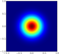
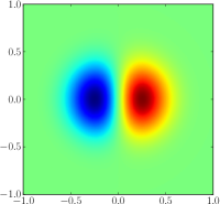
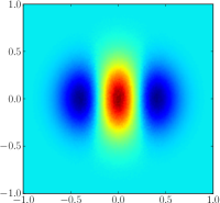
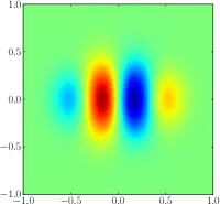
Figure 1: The $i$-th derivative of the likelihood with respect to $g_{1}$ for the posterior distribution at zero shear, where i=0,1,2,3 for the toy model described in the text. The x and y axis are the measured ellipticities for $e_{1}$ and $e_{2}$ respectively, and the color bar saturates positively at red and negatively at blue.

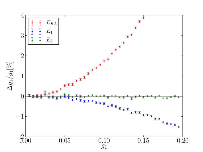
Figure 2: The relative biases in the recovered $g_{1}$ as a function of the input $g_{1}$, with input $g_{2}$ held at zero. For the $E_{1}$ and $E_{3}$ estimators, the error was calculated from the variance in estimates, while for the $E_{AB}$ estimator, it was assumed to be given by the inverse of the second derivative of the posterior.

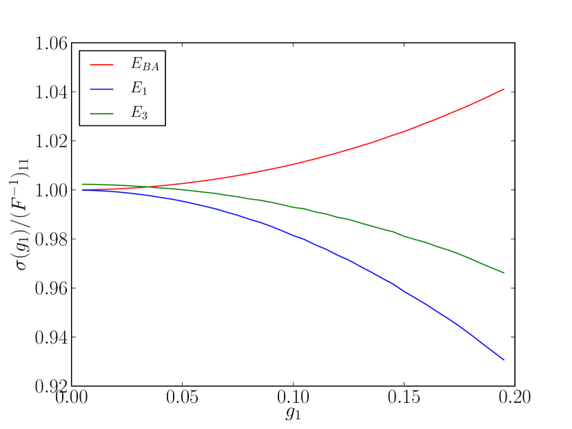
Figure 3: The error of estimators relative to the Fisher matrix prediction at zero shear. For the $E_{1}$ and $E_{3}$ estimators, the error was calculated from the variance in estimates, while for the $E_{AB}$ estimator, it was assumed to be given by the inverse of the second derivative of the posterior.

IV Shear estimation

To apply the formalism above to the problem of shear estimation, we take as a starting point work in Bernstein and Armstrong (2014). We describe the likelihood for shear, $L(\bm{g})$, through its derivatives at zero shear as:

$$P = L(\bm{D}|\bm{g}=0)$$ (27)

$$\mathbf{Q} = \nabla_{\bm{g}}L(\bm{D}|\bm{g})|_{\bm{g}=0}$$ (28)

$$\mathbf{R} = \nabla_{\bm{g}}\nabla_{\bm{g}}L(\bm{D}|\bm{g})|_{\bm{g}=0}$$ (29)

$$\mathbf{S} = \nabla_{\bm{g}}\nabla_{\bm{g}}\nabla_{\bm{g}}L(\bm{D}|\bm{g})|_{\bm{g}=0}$$ (30)

BA14 expand to second order, but we generalize to third. Note that theory parameters here are the two components of shear, and we will use $\bm{g}$ and $\bm{\theta}$ interchangeably below. Derivatives of log likelihood (at zero shear) are thus given by

$$\mathcal{L}_{,i} = \frac{Q_{i}}{P}$$ (31)

$$\mathcal{L}_{,ij} = \frac{R_{ij}}{P}-\frac{Q_{i}Q_{j}}{P^{2}}$$ (32)

$$\mathcal{L}_{,ijk} = \frac{S_{ijk}}{P}-\left(\frac{R_{ij}Q_{k}}{P^{2}}+{\rm cyc}\right)+2\frac{Q_{i}Q_{j}Q_{k}}{P^{3}},$$ (33)

and the $U$ quantities are given simply by

$${}^{1}U_{i} = \frac{Q_{i}}{P}$$ (34)

$${}^{2}U_{ij} = \frac{R_{ij}}{P}$$ (35)

$${}^{3}U_{ijk} = \frac{S_{ijk}}{P}.$$ (36)

BA14 advocate calculating the above quantities for each galaxy. If all galaxies have the same shear, the total probability can be calculated by summing derivatives of the log likelihood. For a sufficient number of galaxies, the likelihood collapses to a Gaussian and the shear can be estimated as

$$\bm{E}_{BA}=-\left(\sum\mathcal{L}_{,ij}\right)^{-1}\left(\sum\mathcal{L}_{,j}\right)$$ (37)

For a sufficiently large number of galaxies $N_{g}$, the sum of second derivatives will approach

$$\sum_{1}^{N_{g}}\mathcal{L}_{,i} \rightarrow N_{g}\left<\mathcal{L}_{,i}\right>_{{\bm{\theta}^{(T)}}}$$ (38)

$$\sum_{1}^{N_{g}}\mathcal{L}_{,ij} \rightarrow N_{g}\left<\mathcal{L}_{,ij}\right>_{{\bm{\theta}^{(T)}}}$$ (39)

Summing the first and second derivatives of the log likelihood is akin to averaging over the true distribution. Therefore, in the limit of an infinite number of galaxies, the estimator will give

$$\left<\bm{E}_{BA}\right>_{{\bm{\theta}^{(T)}}}=-\left(\left<\mathcal{L}_{,ij}(\bm{\theta})\right>_{{\bm{\theta}^{(T)}}}\right)^{-1}\left<\mathcal{L}_{,j}\right>_{\bm{\theta}^{(T)}}$$ (40)

Note that this is subtly different from our estimator, which uses the Fisher matrix, $F_{ij}=-\left<\mathcal{L}_{,ij}(\bm{\theta})\right>_{\bm{\theta}}$, which is the mean of the second derivative of the log likelihood assuming zero shear:

$$\left<\bm{E}_{1}\right>_{{\bm{\theta}^{(T)}}}=-\left(\left<\mathcal{L}_{,ij}(\bm{\theta})\right>_{\bm{\theta}}\right)^{-1}\left<\mathcal{L}_{,j}\right>_{\bm{\theta}^{(T)}}$$ (41)

IV.1 Toy model

To test the above ideas, we use the same toy model that was used in BA14. We draw a source ellipticity from an isotropic unlensed distribution with probability distribution given by

$$P(|\bm{e}^{i}|)\propto(1-|\bm{e}^{i}|^{2})^{2}\exp\left(-\frac{|\bm{e}^{i}|^{2}}{2\sigma^{2}_{p}}\right)$$ (42)

for the magnitude of the ellipticity and a random orientation. The effect of shear is most easily expressed if we cast the intrinsic ellipticity and shear as complex vectors $\bm{e}^{i}=e_{1}^{i}+ie_{2}^{i}$ and $\bm{g}=g_{1}+ig_{2}$. Then the sheared ellipticity vector is given by

$$\bm{e}^{s}=\frac{\bm{e}^{i}-\bm{g}}{1-\bm{g}^{*}\bm{e}^{i}}.$$ (43)

Finally, we add random Gaussian noise to obtain the observed ellipticity $\bm{e}^{o}$:

$$\bm{e}^{o}=\bm{e}^{s}+\bm{\epsilon},$$ (44)

where each component of $\bm{\epsilon}$ is drawn from a truncated Gaussian with variance $\sigma_{n}$ ensuring that $|\bm{e}^{o}|<1$ (in practice random realizations of noise are added to $\bm{e}^{s}$ until $|\bm{e}^{o}|<1$ is satisfied). In this work we limit ourselves to the example of $\sigma_{p}=0.3$ and $\sigma_{n}=0.05$.

IV.2 Third-order estimator

It is clear that at least in the case of this particular problem, symmetry ensures that the second order correction to the estimator vanishes if one expands around zero shear. There are several ways to see this. First, given that shear is a spin-2 quantity, the lowest order scalar one can make is $|\bm{g}|^{2}$ and therefore, one expects the lowest-order correction to an estimate of $\bm{g}$ to scale as $\bm{g}|\bm{g}^{2}|$, which is third order in $\bm{g}$. Second, if one only estimates $g_{1}$, it is natural to expect that the correction to $g_{1}$ must be the same and of opposite sign to the correction to $-g_{1}$ – estimation of shear must be symmetric with respect to mirroring over the origin. Therefore, it cannot receive a $g_{1}^{2}$ correction, and the lowest order correction to the estimator must scale as $g_{1}^{3}$. Note that in Equation 14, this means that ${}^{12}\mathbf{W}=0$.

Therefore, we construct a third-order estimator from quantities ${}^{1}\mathbf{U}$ and ${}^{3}\mathbf{U}$. Again, because of the symmetry of the problem, we construct it assuming the problem is one dimensional, i.e. we are attempting to recover the $g_{1}$ component. In that case all $\mathbf{W}$ quantities are scalar.

Starting with the system of equations:

$$\left<{}^{1}\mathbf{U}\right> = {}^{11}\mathbf{W}\Delta\bm{\theta}+\frac{{}^{13}\mathbf{W}}{6}\Delta\bm{\theta}^{3}+\ldots,$$ (45)

$$\left<{}^{3}\mathbf{U}\right> = {}^{31}\mathbf{W}\Delta\bm{\theta}+\frac{{}^{33}\mathbf{W}}{6}\Delta\bm{\theta}^{3}+\ldots,$$ (46)

it is not difficult to show that, ignoring higher order terms,

$$\frac{{}^{33}\mathbf{W}\left<{}^{1}\mathbf{U}\right>-^{31}\mathbf{W}\left<{}^{3}\mathbf{U}\right>}{{}^{11}\mathbf{W}^{33}\mathbf{W}-^{13}\mathbf{W}^{31}\mathbf{W}}=\Delta\bm{\theta}$$ (47)

Hence, we can write an ansatz:

$$\bm{E}_{3}=\frac{{}^{33}\mathbf{W}^{1}\mathbf{U}-^{31}\mathbf{W}^{3}\mathbf{U}}{{}^{11}\mathbf{W}^{33}\mathbf{W}-^{13}\mathbf{W}^{31}\mathbf{W}}$$ (48)

Since $\mathbf{W}$ quantities do not depend on data, $\left<\bm{E}_{3}\right>=\Delta\bm{\theta}$ and hence this is our third order estimator. For more realistic cases, the rotational symmetry might be broken due to systematic and instrumental effects and for completeness we show how to build a complete 3^rd order estimator in Appendix B.

IV.3 Results for toy model

For this toy example, we can calculate the likelihood and its derivatives simply by brute force Monte Carlo - we can draw a large enough number of samples from the parent distribution such that the gridded values of sampled $\bm{e}$ become a good approximation for the probability distribution. The derivatives are then calculated by finite difference methods from gridded likelihoods. Note that this short-cut is unlikely to work in a more realistic setting due to the higher dimensionality of the problem.

In Figure 1, we plot the $i$-th derivative of the likelihood with respect to $g_{1}$, that is quantities $P$, $Q_{1}$, $R_{11}$, $S_{111}$, showing how the posterior distribution of ellipticities responds to shear at each order.

In Figure 2, we show results for the three estimators discussed in this text. As expected, the $\bm{E}_{BA}$ and $\bm{E}_{1}$ estimators show a quadratic increase in bias as a function of shear, which is mostly removed by the $\bm{E}_{3}$ estimator. In this particular case, our $\bm{E}_{1}$ estimator seems to be performing somewhat better than the original $\bm{E}_{BA}$ estimator, although it is not clear whether this will translate to similar gains in more realistic scenarios. However, the $\bm{E}_{3}$ estimator is designed to be more accurate and performs with a 0.1% relative precision all the way to shears of 0.2, at which point we are well out of the validity of the small shear approximation, and flexion effects Goldberg and Bacon (2005) become important, which are not captured in this toy model.

In Figure 3, we show the error (square root of variance) for the three estimators discussed here, normalized to the Fisher matrix prediction at zero shear. As we can see, both $\bm{E}_{BA}$ and $\bm{E}_{1}$ converge to the Fisher matrix prediction at zero shear, but $\bm{E}_{3}$ is marginally noisier. The effect is small, sub 1%, but clearly detectable. For higher shear, the $\bm{E}_{1}$ and $\bm{E}_{3}$ estimators begin to become slightly less noisy than the zero-shear Fisher prediction. Note that this does not violate the Cramer-Rao bound, since the bound only holds if the true shear is zero.

Finally, we demonstrate explicitly that our estimator can measure correlations. To that end, we draw pairs of galaxies with shear $\bm{g}_{a}$ and $\bm{g}_{b}$, which we randomly choose to follow

$$\left<\bm{g}_{a}\bm{g}_{a}^{T}\right>=\left<\bm{g}_{b}\bm{g}_{b}^{T}\right>=\left(\begin{array}[]{cc}0.05^{2}&0\\ 0&0.05^{2}\\ \end{array}\right)$$ (49)

and

$$\left<\bm{g}_{a}\bm{g}_{b}^{T}\right>=\left(\begin{array}[]{cc}0.00125&0.00075\\ 0.00075&0.00125\\ \end{array}\right).$$ (50)

These pairs of galaxies are modeled using Equations 42, 43, and 44 with $\sigma_{p}=0.3$, $\sigma_{n}=0.05$ to obtain observed values and then with the $E_{3}$ estimator to obtain an estimate. These estimates where then used to obtain the correlations: $\left<\tilde{\bm{g}}_{a}\tilde{\bm{g}}_{b}^{T}\right>_{11}=0.00125319\pm 2.8\times 10^{-6}$ and $\left<\tilde{\bm{g}}_{a}\tilde{\bm{g}}_{b}^{T}\right>_{12}=0.007552\pm 2.8\times 10^{-6}$, consistent with the input values and sub-percent level accurate. Of course, this exercise had to work, so it is really just a sanity check.

V Conclusions

In this paper, we have derived a general framework for generating unbiased estimators. The framework is general and can be used wherever we are measuring a quantity which is perturbatively close to the assumed model. We have shown that the inverse of Fisher matrix multiplied by the first derivative vector is a general formula for a first order unbiased estimator. In special cases such as an optimal quadratic estimator, the estimator is unbiased at all orders. We have applied our framework to the problem of estimating weak lensing shear and constructed a first and third-order estimator.

In the realm of the toy problem of BA14, our third-order estimator is unbiased for all relevant shear magnitudes with a negligible increase in the estimator variance compared to the Fisher prediction at zero shear. In typical weak-lensing analyses, shears are small enough that the first-order estimator may be sufficient. However, there are two cases where third order correction might matter. First, when measuring the cosmic shear power spectrum, an error term proportional to $g^{3}$ will “renormalize” to give a correction to the measured shear power spectrum proportional to $\left<\left|\bm{g}\right|^{2}\right>P_{gg}$, where $P_{gg}$ is the true shear power spectrum. This is of the same order of magnitude as the overall LSST error LSST Science Collaboration et al. (2009). Second, in regions of high-shear, such as those around clusters of galaxies, the third-order estimator will be useful, simply because shear are large-enough that the third order correction matters. The formalism presented here can trivially be extended to the flexion measurement, and it should correctly account for the correlation between shear and flexion. We refrain from making more quantitative statements since it is not clear how realistic the toy model is.

More importantly, we have constructed an estimator which performs as well as the BA14 estimator, but also returns shear estimates for individual galaxies, which makes it usable in direct measurements of the $n$-point function of the shear field.

We also note that to some extent the main problem with shear measurements is not the underlying framework, which is the focus of this paper, but the bias arising from inadequate modeling of the properties of unlensed galaxies, and it might turn out that these problems are best solved using very phenomenological approaches as those discussed in e.g. Miller et al. (2007); Refregier and Amara (2013).

Putting this estimator into practice might be more complicated. In particular, in its current incarnation, it gives the same weight to all galaxies, while we know that this will not hold in reality. The correct way to solve this problem is to separate galaxies into sub-classes in a way that does not correlate (or negligibly correlates) with the underlying shear. A separate estimator can be constructed for each class, and the Fisher matrix is the appropriate weight. We leave testing of this framework in more realistic settings for the future work.

Appendix A Example of bias of ML estimator

Here we give a concrete example of a likelihood for which the maximum likelihood estimator is biased. In general, this happens with asymmetric likelihoods. Consider:

$$L=x\lambda^{2}e^{-\lambda x},$$ (51)

where $x>0$ is the “data” and $\lambda>0$ is the theory parameter. Given exactly one measurement $x$, the maximum likelihood estimator (i.e. the estimator where one would end up upon iterations of Newton-Raphson steps) is

$$E_{ML}=\frac{2}{x},$$ (52)

whose expectation value is $2\lambda$, i.e, wrong by a factor of two. Expanding around $\lambda=l$, our first order estimator is given by

$$E_{1}=\frac{l(4-lx)}{2}$$ (53)

which is unbiased up to quadratic order in $\lambda-l$. Interestingly,

$$E=\frac{1}{x}$$ (54)

is unbiased at all orders and is neither ML nor our perturbative estimator.

Appendix B General 3^rd order estimator

For completeness we demonstrate how to build a full third order estimator. This procedure can be trivially generalized to any order. We write the Equation (9) to up to third order in an “unrolled” matrix form

$$\left<U\right>=Wg,$$ (55)

where we have, assuming that there are two theory parameters that we want to recover ($g_{1}$ and $g_{2}$),

$$U=\left[\begin{array}[]{c}\left<{}^{1}U_{1}\right>\\ \left<{}^{1}U_{2}\right>\\ \left<{}^{2}U_{11}\right>\\ \left<{}^{2}U_{12}\right>\\ \left<{}^{2}U_{22}\right>\\ \left<{}^{3}U_{111}\right>\\ \left<{}^{3}U_{112}\right>\\ \left<{}^{3}U_{122}\right>\\ \left<{}^{3}U_{222}\right>\end{array}\right]$$ (56)

and

$$W=\left[\begin{array}[]{ccccccccc}{}^{11}W_{1|1}&{}^{11}W_{1|2}&{}^{12}W_{1|11}&{}^{12}W_{1|12}&{}^{12}W_{1|22}&{}^{13}W_{1|111}&{}^{13}W_{1|112}&{}^{13}W_{1|122}&{}^{13}W_{1|222}\\ {}^{11}W_{2|1}&{}^{11}W_{2|2}&{}^{12}W_{2|11}&{}^{12}W_{2|12}&{}^{12}W_{2|22}&{}^{13}W_{2|111}&{}^{13}W_{2|112}&{}^{13}W_{2|122}&{}^{13}W_{2|222}\\ {}^{21}W_{11|1}&{}^{21}W_{11|2}&{}^{22}W_{11|11}&{}^{22}W_{11|12}&{}^{22}W_{11|22}&{}^{23}W_{11|111}&{}^{23}W_{11|112}&{}^{23}W_{11|122}&{}^{23}W_{11|222}\\ {}^{21}W_{12|1}&{}^{21}W_{12|2}&{}^{22}W_{12|11}&{}^{22}W_{12|12}&{}^{22}W_{12|22}&{}^{23}W_{12|111}&{}^{23}W_{12|112}&{}^{23}W_{12|122}&{}^{23}W_{12|222}\\ {}^{21}W_{22|1}&{}^{21}W_{22|2}&{}^{22}W_{22|11}&{}^{22}W_{22|12}&{}^{22}W_{22|22}&{}^{23}W_{22|111}&{}^{23}W_{22|112}&{}^{23}W_{22|122}&{}^{23}W_{22|222}\\ {}^{31}W_{111|1}&{}^{31}W_{111|2}&{}^{32}W_{111|11}&{}^{32}W_{111|12}&{}^{32}W_{111|22}&{}^{33}W_{111|111}&{}^{33}W_{111|112}&{}^{33}W_{111|122}&{}^{33}W_{111|222}\\ {}^{31}W_{112|1}&{}^{31}W_{112|2}&{}^{32}W_{112|11}&{}^{32}W_{112|12}&{}^{32}W_{112|22}&{}^{33}W_{112|111}&{}^{33}W_{112|112}&{}^{33}W_{112|122}&{}^{33}W_{112|222}\\ {}^{31}W_{122|1}&{}^{31}W_{122|2}&{}^{32}W_{122|11}&{}^{32}W_{122|12}&{}^{32}W_{122|22}&{}^{33}W_{122|111}&{}^{33}W_{122|112}&{}^{33}W_{122|122}&{}^{33}W_{122|222}\\ {}^{31}W_{222|1}&{}^{31}W_{222|2}&{}^{32}W_{222|11}&{}^{32}W_{222|12}&{}^{32}W_{222|22}&{}^{33}W_{222|111}&{}^{33}W_{222|112}&{}^{33}W_{222|122}&{}^{33}W_{222|222}\\ \end{array}\right]$$ (57)

and

$$g=\left[\begin{array}[]{c}g_{1}\\ g_{2}\\ g_{1}g_{1}\\ 2\times g_{1}g_{2}\\ g_{2}g_{2}\\ g_{1}g_{1}g_{1}\\ 3\times g_{1}g_{1}g_{2}\\ 3\times g_{1}g_{2}g_{2}\\ g_{2}g_{2}g_{2}\\ \end{array}\right].$$ (58)

In expression for $W$, we have used a pipe symbol to separate indices corresponding to the left and right sides of the equation. Solving this matrix equation for the vector $g$. We have

$$g=W^{-1}\left<U\right>$$ (59)

We can now write an ansatz for the estimator:

$$E=W^{-1}U$$ (60)

Since $W$ does not depend on data, it trivially follows that

$$\left<E\right>=W^{-1}\left<U\right>=g$$ (61)

Hence, the first two components of $E$, namely $E_{1}$ and $E_{2}$ are unbiased estimators for the first two components of $g$, that is $g_{1}$ and $g_{2}$. In other words, the linear algebra has given us the particular linear combination of $U$ quantities which average to $g_{1}$ and $g_{2}$ without any contribution from terms quadratic and cubic in $g$.