The Initial Flow of Classical Gluon Fields in Heavy Ion Collisions

Abstract

Using analytic solutions of the Yang-Mills equations we calculate the initial flow of energy of the classical gluon field created in collisions of large nuclei at high energies. We find radial and elliptic flow which follows gradients in the initial energy density, similar to a simple hydrodynamic behavior. In addition we find a rapidity-odd transverse flow field which implies the presence of angular momentum and should lead to directed flow in final particle spectra. We trace those energy flow terms to transverse fields from the non-abelian generalization of Gauss’ Law and Ampére’s and Faraday’s Laws.

1 Introduction

At asymptotically large energies (or small Bjorken-$x$) the gluon fields in hadrons and nuclei approach a state of nuclear matter generally referred to as color glass condensate (CGC) [1, 2]. The transverse gluon density saturates at a value $\sim Q_{s}^{-2}$ characterized by a saturation scale $Q_{s}$. In this limit large occupation numbers permit a quasi-classical treatment of the gluon field which is the approximation known as the McLerran-Venugopalan (MV) model [3, 4]. The saturation scale $Q_{s}$ grows with the size of the nucleus $\sim A^{1/3}$. Hence high energy nuclear collisions at the Relativistic Heavy Ion Collider (RHIC) and the Large Hadron Collider (LHC) offer unique opportunities to study CGC.

Here we report on results from a calculation which solves the classical gluon field (Yang-Mills) equations employing an expansion in powers of the proper time $\tau=\sqrt{t^{2}-z^{2}}$ after the collision. We focus on the transverse Poynting vector $S^{i}=T^{0i}$, $i=1,2$ of the gluon field, where $T^{\mu\nu}$ is the energy momentum tensor. $S^{i}$ describes the initial transverse flow of energy of the gluon field, but we expect this flow to translate into hydrodynamic flow of quark gluon plasma once the system thermalizes. Our results have first been reported in detail in [5, 6].

2 Color Glass Condensate

We seek solutions of the classical Yang-Mills equations

$$\left[D_{\mu},F^{\mu\nu}\right]=J^{\nu}$$ (1)

where the $SU(3)$-current $J^{\mu}$ is generated by two transverse charge distributions $\rho_{1}(\vec{x}_{\perp})$ and $\rho_{2}(\vec{x}_{\perp})$ moving on the $+$ and $-$ light cone respectively. The $\rho_{i}$ describe the $SU(3)$ charge distributions of the large-$x$ partons in the colliding nuclei which generate the small-$x$ gluon field. Typically these equations are solved numerically in the forward light cone ($\tau\geq 0$) [7, 8, 9].

However, it is possible to obtain an analytic recursive solution as well, as first described in [10]. To that end one employs a power series for the gauge potential $A^{\mu}$ in the forward light cone,

$$A(\tau,\vec{x}_{\perp}) =\sum_{n=0}^{\infty}\tau^{n}A_{(n)}(\vec{x}_{\perp})\,,$$ (2)

$$A_{\perp}^{i}(\tau,\vec{x}_{\perp}) =\sum_{n=0}^{\infty}\tau^{n}A_{\perp(n)}^{i}(\vec{x}_{\perp})\,,$$ (3)

where in light cone notation $A^{\pm}=\pm x^{\pm}A$. The leading terms are given by boundary conditions on the light cone [11]

$$A_{\perp(0)}^{i} =A_{1}^{i}+A_{2}^{i}\,,$$ (4)

$$A_{(0)} =-\frac{ig}{2}\left[A_{1}^{i},A_{2}^{i}\right]\,,$$ (5)

where $A^{i}_{1}$ and $A_{2}^{i}$ are the gauge potentials in nucleus 1 and 2 (generated by charges $\rho_{1}$ and $\rho_{2}$), respectively, before the collision. The recursion relation for coefficients of even powers $n$ ($n>1$), are

$$A_{(n)}= \frac{1}{n(n+2)}\sum_{k+l+m=n-2}\left[D^{i}_{(k)},\left[D^{i}_{(l)},A_{(m)}\right]\right],$$ (6)

$$A^{i}_{\perp(n)}= \frac{1}{n^{2}}\left(\sum_{k+l=n-2}\left[D^{j}_{(k)},F^{ji}_{(l)}\right]+ig\sum_{k+l+m=n-4}\left[A_{(k)},[D^{i}_{(l)},A_{(m)}]\right]\right)\,,$$ (7)

while all odd coefficients vanish. The convergence radius of this series in $\tau$ will generally be of order $1/Q_{s}$, but for example the series recovers the known solution for the abelian case for all times [12].

The physical fields $F^{\mu\nu}$ can be expanded in $\tau$ as well and can be computed order by order from $A^{\mu}$. The dominant fields for small times, i.e. at order $\mathcal{O}(\tau^{0})$, are the longitudinal chromo-electric and -magnetic fields [10, 13]

$$E_{(0)}=F^{+-}_{(0)} =ig\left[A_{1}^{i},A_{2}^{i}\right]\,,$$ (8)

$$B_{(0)}=F^{21}_{(0)} =ig\epsilon^{ij}\left[A_{1}^{i},A_{2}^{j}\right]\,.$$ (9)

From this result one can calculate an initial energy density $\epsilon_{0}=T^{00}_{(0)}$. After averaging over charge densities $\rho_{i}$ one obtains an event-averaged energy density [14, 12]

$$\varepsilon_{0}(\vec{x}_{\perp})=2\pi\alpha_{s}^{3}\frac{N_{c}}{N_{c}^{2}-1}\mu_{1}(\vec{x}_{\perp})\mu_{2}(\vec{x}_{\perp})\ln^{2}\frac{Q^{2}}{\hat{m}^{2}}\,.$$ (10)

Here the usual assumptions of the MV model have been applied, i.e. the $\rho_{i}$ follow Gaussian distributions and $\mu_{1}$ and $\mu_{2}$ determine the average squared charge distribution in each nucleus. $Q$ and $\hat{m}$ are UV and IR cutoffs respectively.

3 Transverse Fields and Transverse Flow

Transverse electric and magnetic fields enter at order $\mathcal{O}(\tau^{1})$ in the power series of $F^{\mu\nu}$. The corresponding coefficients can be computed to be [6]

$$E^{i}_{(1)} =-\frac{1}{2}\left(\sinh\eta[D^{i},E_{0}]+\cosh\eta\,\epsilon^{ij}[D^{j},B_{0}]\right)$$ (11)

$$B^{i}_{(1)} =\frac{1}{2}\left(\cosh\eta\,\epsilon^{ij}[D^{j},E_{0}]-\sinh\eta[D^{i},B_{0}]\right)\,.$$ (12)

Here $\eta$ is the space-time rapidity. One can readily verify that these expressions are simply the $SU(3)$ analogs of Gauss’ Law and Faraday’s and Ampére’s Laws. More specifically, the $\eta$-odd terms emerge naturally as a consequence of Gauss’ Law, see Fig. 1.

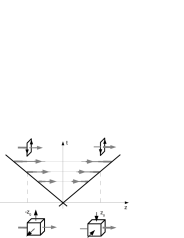
Figure 1: Schematic sketch of Gauss’ Law (cubes) and Ampére’s and Faraday’s Laws (loops) for positive and negative values of the longitudinal coordinate $z$. The initial longitudinal electric and magnetic fields in the forward light cone diminish as functions of $t$ and $z$. Transverse fields due to Gauss’ Law will have different signs for positive and negative $z$, while transverse fields due to Ampére’s and Faraday’s Law are symmetric in $z$. The abelian version is shown here, see [6] for details.

Fig. 2 shows a typical configuration of transverse fields (in the abelian case for simplicity) for randomly seeded longitudinal fields $E_{0}$ and $B_{0}$. At rapidity $\eta=0$ the transverse fields are divergence-free, i.e. only closed field lines due to Ampére’s and Faraday’s Law appear. At $\eta=1$ contributions from Gauss’ Law are present as well.

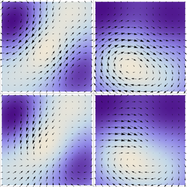
Figure 2: Transverse electric fields (left panels) and magnetic fields (right panels) at $\eta=0$ (upper panels) and $\eta=1$ (lower panels) for a random distribution of initial longitudinal electric (shown as background in the right panels) and magnetic fields (left panels). At $\eta=0$ the fields are divergence-free. The abelian case is shown here, see [6] for details.

We are now able to calculate the flow of energy due to transverse fields. The transverse Poynting vector $S^{i}$ receives its first contribution in the power series of $T^{\mu\nu}$ at order $\mathcal{O}(\tau^{1})$. I.e. transverse flow in color glass sets in linearly in time,

$$T^{0i}=\frac{\tau}{2}\cosh\eta\,\alpha^{i}+\frac{\tau}{2}\sinh\eta\,\beta^{i}\,.$$ (13)

There is a rapidity-even part $\alpha^{i}$ and a rapidity-odd contribution $\beta^{i}$ to the Poynting vector which are given by [6]

$$\alpha^{i}=-\nabla^{i}\varepsilon_{0}\quad\,,\qquad\beta^{i}=\epsilon^{ij}\left([D^{j},B_{0}]E_{0}-[D^{j},E_{0}]B_{0}\right)\,.$$ (14)

The rapidity-odd flow is expected from the existence of rapidity-odd gauge fields, however it is more of a surprise when one approaches the topic of early flow from a purely phenomenological point of view. $\alpha^{i}$ corresponds to energy flow as expected from hydrodynamic expansion, following the gradient of energy. On the other hand $\beta^{i}$ is determined by the gauge field structure underlying the energy density.

After averaging over color charges $\rho_{i}$ we obtain event-averaged transverse flow fields [6]

$$\alpha^{i}=-\varepsilon_{0}\frac{\nabla^{i}\left(\mu_{1}\mu_{2}\right)}{\mu_{1}\mu_{2}}\quad,\qquad\beta^{i}=-\varepsilon_{0}\frac{\mu_{2}\nabla^{i}\mu_{1}-\mu_{1}\nabla^{i}\mu_{2}}{\mu_{1}\mu_{2}}\,.$$ (15)

We omit the notation $\langle\ldots\rangle$ for event-averaged quantities if no confusion can arise. Fig. 3 shows the initial event-averaged transverse flow field in Au+Au collisions at impact parameter $b=6$ fm for two space-time rapidities $\eta$.

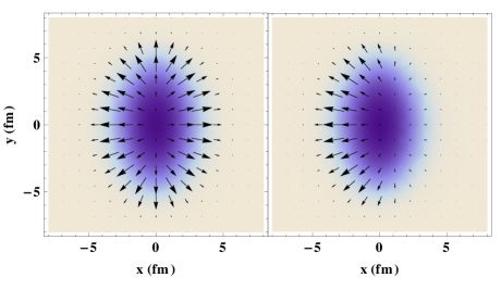
Figure 3: Transverse flow of energy $T^{0i}$ (black arrows; arbitrary units) and energy density $\varepsilon_{0}$ (shading) in the transverse plane for Au+Au collisions at impact parameter $b=6$ fm. The nucleus with center located at $x=3$ fm travels into the plane (the positive $\eta$-direction). Left Panel: $\eta=0$. Right Panel: $\eta=1$.

One can clearly see a radial and elliptic flow pattern for $\eta=0$ which is qualitatively similar to what would develop in hydrodynamics. At $\eta=1$ the rapidity-odd flow $\beta^{i}$ becomes comparable to $\alpha^{i}$ and we notice that the gluon energy flow develops a preferred direction. This is akin to directed flow $v_{1}$. We can see this more clearly in Fig. 4 where the transverse flow is shown as a function of $x$ and $\eta$ in the plane $y=0$. The gluon field expands more rapidly in the wake of a passing nucleus.

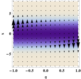
Figure 4: Same as Fig. 3 but plotted in the $\eta-x$-plane defined by $y=0$. A flow pattern akin to directed flow emerges. The nucleus with center at $x=3$ fm is traveling to the right.

Interesting flow patterns can also be observed for asymmetric collision systems. Fig. 5 shows the transverse flow in the $x-\eta$-plane for Au+Cu collisions for two different impact parameters. Once again energy flow is larger in the wake of the spectators of the larger nucleus, leading to a strong asymmetry between forward and backward rapidities.

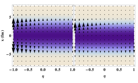
Figure 5: The same as Fig. 4 for Au+Cu (Au traveling to the right). Left Panel: $b=0$ fm. Right Panel: $b=2$ fm.

4 Summary and Discussion

We have calculated the initial flow of energy of the classical gluon field in high energy nuclear collisions. Our results are valid up to roughly a time $\sim 1/Q_{s}$ after the collision. The gluon field is expected to decohere and thermalize soon after. Energy and momentum conservation will translate the flow fields found here into hydrodynamic flow which then will develop further and eventually freeze out into particle flow. We expect the rapidity-odd pre-equilibrium flow $\beta^{i}$ to translate into (rapidity-odd) directed flow $v_{1}$ of particles. The sign and general rapidity dependence of $\beta^{i}$ are qualitatively consistent with experimental results [6] but a more quantitative statement would require a follow-up 3+1-D viscous hydrodynamic simulation.

One can also interpret the flow term $\beta^{i}$ for symmetric collision systems with finite impact parameters $b$ with the inevitable presence of angular momentum $L_{y}$ (perpendicular to the reaction plane). The initial gluon field transfers a part of the angular momentum in the system before the collision onto the fireball after the collision [15, 16]. There it leads to a rotation of the fireball and possibly to vorticity in the quark gluon fluid.

Another very interesting result is the flow found for asymmetric A+B collision systems. The field $\beta^{i}$ specifically relies on the fact that classical gauge fields are the relevant degrees of freedom and one could speculate that observables exist in asymmetric collision systems which are unique signatures for the flow of gauge fields. A further investigation into this direction would be worthwhile.

In the future we plan to use our results on pre-equilibrium flow in viscous hydrodynamic calculations. Preliminary results show that key features of $T^{\mu\nu}$, like angular momentum, readily translate into hydrodynamic fields (local energy density,fluid velocity, shear stress, etc.) in a rapid thermalization scenario [17, 9].

This work was supported by the U.S. National Science Foundation through CAREER grant PHY-0847538, and by the JET Collaboration and DOE grant DE-FG02-10ER41682.

References

References

- [1] Iancu E and Venugopalan R 2004 Quark gluon plasma vol 3, eds. R C Hwa and X. N. Wang (World Scientific) p 249 (Preprint hep-ph/0303204)
- [2] Gelis F, Iancu E, Jalilian-Marian J and Venugopalan R 2010 Ann. Rev. Nucl. Part. Sci. 60 463
- [3] McLerran L D and Venugopalan R 1994 Phys. Rev. D 49 3352
- [4] McLerran L D and Venugopalan R 1994 Phys. Rev. D 49 2233
- [5] Chen G and Fries R J 2013 J. Phys.: Conf. Ser. 446 012021
- [6] Chen G and Fries R J 2013 Phys. Lett. B 723 417
- [7] Krasnitz A and Venugopalan R 2001 Phys. Rev. Lett. 86 1717
- [8] Lappi T 2003 Phys. Rev. C 67 054903
- [9] Schenke B, Tribedy P and Venugopalan R 2012 Phys. Rev. Lett. 108 252301
- [10] Fries R J, Kapusta J I and Li Y 2006 Preprint nucl-th/0604054
- [11] Kovner A, McLerran L D and Weigert H 1995 Phys. Rev. D 52 3809
- [12] Chen G, Fries R J, Kapusta J I, Li Y 2014 In preparation
- [13] Lappi T and McLerran L 2006 Nucl. Phys. A 772 200
- [14] Lappi T 2006 Phys. Lett. B 643 11
- [15] Liang Z T and Wang X N 2005 Phys. Rev. Lett. 94 102301, Erratum-ibid. 96 039901
- [16] Csernai L P, Magas V K, Stocker H and Strottman D D 2011 Phys. Rev. C 84 024914
- [17] Fries R J, Kapusta J I and Li Y 2006 Nucl. Phys. A 774 861