Interaction-induced backscattering in short quantum wires

Abstract

We study interaction-induced backscattering in clean quantum wires with adiabatic contacts exposed to a voltage bias. Particle backscattering relaxes such systems to a fully equilibrated steady state only on length scales exponentially large in the ratio of bandwidth of excitations and temperature. Here we focus on shorter wires in which full equilibration is not accomplished. Signatures of relaxation then are due to backscattering of hole excitations close to the band bottom which perform a diffusive motion in momentum space while scattering from excitations at the Fermi level. This is reminiscent to the first passage problem of a Brownian particle and, regardless of the interaction strength, can be described by an inhomogeneous Fokker-Planck equation. From general solutions of the latter we calculate the hole backscattering rate for different wire lengths and discuss the resulting length dependence of interaction-induced correction to the conductance of a clean single channel quantum wires.

I Introduction

The study of equilibration in many-particle quantum systems has moved into the focus of recent research interest. Polkovnikov2011 ; Imambekov2012 This interest has been partially driven by the impressive experimental progress in realizing and manipulating many-particle quantum systems. One remarkable example is the recent cold atom realization of the Tonks Girardeau gas, which allowed to study the suppression of relaxation in an integrable many-body system. weiss

Clean mesoscopic quantum wires provide another example of systems in which equilibration is strongly suppressed. Barak2010 Specifically, in clean single channel quantum wires equilibration is due to backscattering of excitations which occur at energies of the order of their bandwidth $\Delta$. feq ; peq ; eqLL ; GLL ; eqWC As a consequence, the equilibration rate displays activated temperature dependence, $\tau_{\rm eq}^{-1}\propto e^{-\Delta/T}$ and, when exposed to a finite voltage bias, a fully equilibrated steady state only occurs in wires exceeding an exponentially large length scale $\ell_{\rm eq}\propto e^{\Delta/T}$.

In shorter wires, $L\ll\ell_{\rm eq}$, effects of equilibration on electrons at the Fermi level can be neglected and signatures of relaxation are due to backscattering of particles close to the band bottom. Lunde2007 ; AZT-PRB11 The key process for relaxation in this case is one in which a thermally activated hole overcomes, as it scatters from excitations at the Fermi level, a barrier of energetically unfavorable states at the band bottom via random small steps in momentum space. This picture of a Brownian particle applies regardless of the interaction strength and thus opens the possibility to study equilibration of one-dimensional fermions beyond the weak interaction regime.

Strongly interacting electrons are commonly described within the Luttinger liquid framework and previous work has studied scattering of a Brownian particle in a homogeneous Luttinger liquid. CastroFisher The focus of the present paper is on the equilibration in voltage biased quantum wires. Here, the nature of the specific boundary conditions requires to address a space-dependent, i.e. inhomogeneous problem.

The outline of the paper is as follows. Section II introduces the backscattering rate of holes and reviews how a finite rate affects the conductance of the wire. In Section III we discuss the relevant kinetic equation. Solutions of the latter, the resulting backscattering rate and interaction-induced correction to the conductance of the wire are discussed in Sections IV and V. Details of the calculations are relegated to the appendices.

II Backscattering rate

Consider interacting electrons in a clean one-dimensional quantum wire adiabatically connected to two-dimensional reservoirs via fully transparent contacts. A non-equilibrium situation arises when reservoirs at left and right contacts are biased by a finite voltage $V$. Then, right- and left-moving electrons injected into the wire from the left and right reservoir, respectively, are at different equilibria, see Fig. 1. In the absence of interactions the conductance of the wire reads

$$G_{0}=G_{q}\left(1-e^{-\mu/T}\right),$$ (1)

where $G_{q}=2e^{2}/h$ is the quantum of conductance, and $\mu$ is the chemical potential. Accounting for interactions within the Luttinger liquid framework, the conductance of a finite wire remains $G_{q}$. maslov ; Ponomarenko ; Safi While electrons inside a realistic voltage biased wire relax towards a new steady state, excitations within the Luttinger liquid model have an infinite life time. To study effects of equilibration on finite temperature transport coefficients, one thus has to go beyond the Luttinger liquid model. As we discuss below, this can be accomplished even if interactions are strong.

Taking into account relaxation into a new steady state, the latter can be characterized in terms of a local backscattering rate $\dot{n}^{R}(x)$ of fermions. In the limit of weak interactions, $n^{R}(x)={2\over L}\sum_{p>0}f_{p,x}$ is the density of right-moving electrons. The dot here and in the following refers to the total time derivative, $f_{p,x}$ is the Fermi distribution of (weakly interacting) electrons and the factor $2$ is due to spin-degeneracy. The total backscattering rate of electrons is then $\dot{N}^{R}=\int_{-L/2}^{L/2}dx\,\dot{n}^{R}(x)$ and a finite rate results from backscattering of highly excited holes close to the band bottom, see Fig. 2.

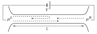
Figure 1: One-dimensional quantum wire of length $L$, adiabatically connected to two-dimensional reservoirs which are kept at different equilibria characterized by chemical potentials $\mu^{L/R}=\mu\pm eV/2$. Right- and left-moving electrons enter the wire from different reservoirs and relax towards a new equilibrium state through interaction-induced backscattering of particles.

The above picture readily generalizes to strong interactions. Indeed, one can extend the concept of a hole excitation to arbitrary interaction strengths by noting that for a system with concave spectrum the lowest energy excitation at a given momentum $Q$ is a hole. Imambekov2012 ; Matveev2013 Even though interactions renormalize its spectrum $\epsilon_{Q}$, the hole remains a spin-$1/2$ excitation with a two-fold degeneracy of the energy levels protected by spin-rotation symmetry. The energy spectrum is periodic, $\epsilon_{Q}=\epsilon_{Q+2p_{F}}$, and quasi-momenta of hole excitations may thus be restricted to the first Brillouin zone $|Q|<p_{F}$. Building on this observation, a backscattering event corresponds to an umklapp process in which the highly excited hole crosses the edge of the Brillouin zone. Notice here that the edge of the Brillouin zone corresponds to the band bottom of the spectrum of the non-interacting fermions, and both terms will be used synonymously below, see also Fig. 2. In particular, in both pictures the relaxation is due to processes taking place at the bottom of the band, i.e. involving highly excited holes. To simplify notation, in the subsequent discussion instead of the momentum of the hole $Q$ measured from the nearest Fermi point we will use the momentum of the missing electron near the bottom of the band, $p=p_{F}{\rm sgn}(Q)-Q$.

Regardless of the interaction strength the total backscattering rate of holes is calculated in terms of the hole distribution $g_{p,x}$,

$$\dot{N}^{R} =-2\int_{-L/2}^{L/2}dx\,\sum_{p>0}\dot{g}_{p,x}.$$ (2)

In the short wires considered in this paper the backscattering rate (2) is controlled by momenta close to the band bottom $|p|\ll p_{F}$. We will discuss the hole occupation numbers $g_{p,x}$ in the following sections. The factor of 2 in Eq. (2) again results from spin-degeneracy, and the minus sign from expressing the backscattering rate in terms of the hole distribution. A finite backscattering rate manifests in a reduced steady state current,peq ; GLL

$$I=G_{0}V+e\dot{N}^{R},$$ (3)

corresponding to a conductance which differs from that of a non-interacting system (1),

$$G=G_{0}+\delta G,\quad\delta G={e\dot{N}^{R}\over V}.$$ (4)

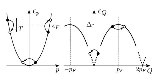
Figure 2: Left: Spectrum of weakly interacting electrons. Relaxation at weak interactions occurs via three-particle scattering processes in the course of which a highly excited hole at the band bottom is backscattered. Right: The concept of backscattering of a highly excited hole also applies at strong interactions. The energy of a hole excitation $\epsilon_{Q}$ is shown as a function of its momentum $Q$. First Brillouin zone $|Q|<p_{F}$ corresponds to the momentum $Q$ of the hole measured from the nearest Fermi point. As a result of many collisions with low energy bosonic excitations the latter may increase its momentum $Q$ and enter the second Brillouin zone, after which it is more likely to fall toward $Q=2p_{F}$ than to return to the vicinity of $Q=0$. Each backscattering event thus corresponds to an umklapp process in which a highly excited hole crosses the edge of Brillouin zone (dashed lines).

The backscattering rate (2) recently has been studied in the limit of relatively short Lunde2007 ; AZT-PRB11 ($L\ll\ell_{0}$) and relatively long ($L\gg\ell_{1}$) wires.peq While the characteristic scales $\ell_{0}$ and $\ell_{1}$ are discussed in detail below, we mention here that the condition $L\lesssim\ell_{0}$ defines a quasi-ballistic regime, in which a hole at the bottom of the band typically scatters at most once from excitations at the Fermi level during its passage through the wire. On the other hand, the condition $L\gg\ell_{1}$ defines a homogeneous diffusive regime where the hole suffers from many collisions granting fully diffusive dynamics in momentum space on a scale set by temperature. In both cases the distribution function of the holes at the bottom of the band is space-independent. That is, one effectively deals with a homogeneous problem and consequently linear dependences $\dot{N}^{R}\propto L$ are found. Slopes, however, are parametrically different in the quasi-ballistic and homogenous diffusive regimes. One should therefore expect a nontrivial length dependence $\delta G(L)$ in the intermediate regime which at low temperatures of interest defines a wide region of length scales $\ell_{0}\ll L\ll\ell_{1}$ specified below. As we discuss next, this condition defines an inhomogeneous diffusive regime, in which the typical range of diffusive dynamics in momentum space is set by the length of the wire. This latter is addressed within an inhomogeneous Fokker-Planck equation.

III Fokker-Planck equation

The Fokker-Planck equation (FPE) describes the paradigmatic situation in which a heavy ‘Brownian’ particle propagates in a dilute gas of light particles. Collisions between heavy and light particles then lead to a diffusive motion of the former. In our context, the typical momentum $\delta p$ transferred in a collision between a hole at the band bottom and thermally excited electron-hole excitations (plasmons) is restricted due to Fermi blocking to be of the order of $\delta p\sim T/v$, where $v$ is the velocity of excitations at the Fermi level. Below we consider the case in which the dispersion of a hole at the bottom of the band is quadratic,

$$\epsilon_{p}=\Delta-{p^{2}\over 2m^{*}},$$ (5)

with $m^{*}$ being the effective mass of the hole. We then encounter the above situation at low enough temperatures where the typical momentum of the hole $p_{0}\sim\sqrt{m^{*}T}\gg\delta p$, see also Fig. 3.

Formally, we start out from the Boltzmann equation

$${p\over m^{*}}\partial_{x}g_{p,x}=I_{p,x}[g]$$ (6)

for the hole distribution $g_{p,x}=1-f_{p,x}$ in a steady state $\partial_{t}g_{p,x}=0$. Employing the small parameter $\delta p/p_{0}\ll 1$ one may perform a Kramers-Moyal expansion and approximate the collision integral by the Fokker-Planck form

$$I_{p,x}[g]\simeq-\partial_{p}\left(A(p)g_{p,x}-{1\over 2}\partial_{p}[B(p)g_{p,x}]\right).$$ (7)

The Fokker-Planck operator describes an interplay of drift and diffusion which sends the system into the new steady state. Coefficients $A(p)$ and $B(p)$ in Eq. (7) are model specific functions. In all cases of interest, variation of the coefficient $B(p)$ occurs on a momentum scale much larger than $p_{0}$, and it may thus be approximated by a constant $B(p)=B$. Employing common statistical mechanics arguments, we further know that in a homogeneous equilibrium situation, $eV=0$, the dilute hole at the band bottom is described by a Boltzmann distribution. This fixes $A(p)=Bp/(2m^{*}T)$, and the (dilute) hole distribution thus follows the space-dependent FPE, also known as Kramers equation kramers ; risken

$${p\over m^{*}}\partial_{x}g_{p,x} =\frac{B}{2}\partial_{p}\left(-{pg_{p,x}\over m^{*}T}+\partial_{p}g_{p,x}\right).$$ (8)

All microscopic details are stored in the single constant $B$, which physically speaking has the meaning of a diffusion constant in momentum space. It can be explicitly calculated in the special cases of either weak or strong interactions. peq ; eqWC ; AZT-PRB11 ; MatveevAndreevKlironomos Interestingly, one can also obtain a phenomenological expression for $B$ in terms of the spectrum of the mobile impurity (hole) in the Luttinger liquid. eqLL ; Matveev2013 ; Matveev2012 Inhomogeneity in Eq. (8) is induced by the boundary conditions taking into account the finite voltage bias. For a dilute hole at the band bottom the latter can be approximated by a classical Boltzmann form

$$g_{p,-L/2} = e^{\epsilon_{p}/T}e^{-(\Delta+eV/2)/T},\quad\mbox{for $p>0$},$$ (9a)

$$g_{p,L/2} = e^{\epsilon_{p}/T}e^{-(\Delta-eV/2)/T},\quad\mbox{for $p<0$},$$ (9b)

where $\Delta$ is the bandwidth of the hole excitations, see Eq. 5.

While the above expressions (9a) and (9b) are obvious in the limit of weak interactions, let us notice that independent of the interaction strength the occupation of (dilute) high-energy excitations in a fluid at rest is given by the Boltzmann factor $g_{Q}=e^{-\epsilon_{Q}/T}$, where $\epsilon_{Q}$ the excitation spectrum. A finite voltage bias sets the fluid in motion and changes the excitation spectrum of the Galilean invariant system in the stationary frame according to $\epsilon_{Q}\to\epsilon_{Q}+uQ$ where $u=I/(en)$ is the fluid velocity expressed in terms of the electric current $I$ and the particle density $n$. Restricting then $|Q|\leq p_{F}$ to the first Brillouin zone and measuring momenta from the zone boundary we substitute $Q=p_{F}\operatorname{sgn}(p)-p$, where for our purposes $|p|\sim\sqrt{m^{*}T}\ll p_{F}$. Substituting further particle density $n=4p_{F}/h$ and current $I\simeq G_{q}V$, one arrives at the above boundary conditions.

Using Eq. (7) one finds the backscattering rate in the Fokker-Planck approximation

$$\dot{N}^{R}={B\over h}\int_{-L/2}^{L/2}dx\,\left(\partial_{p}g_{p,x}\right)|_{p=0}.$$ (10)

Here $\left(\partial_{p}g_{p,x}\right)|_{p=0}$ affords the interpretation of the current of the holes in momentum space through the band bottom, resulting in the interaction-induced correction $\delta G(L)$ to the conductance of non-interacting electrons, see Eq. (4).

Before we start a detailed analysis of the Kramers equation (8), it is instructive to obtain the characteristic scales of distance $\ell_{1}$ and momentum $p_{0}$ inherent to it. Assuming that the expression in the left-hand side of Eq. (8) is of the same order of magnitude as each of the terms in the right-hand side, we obtain

$$\frac{p_{0}}{m^{*}\ell_{1}}\sim\frac{B}{m^{*}T}\sim\frac{B}{p_{0}^{2}}.$$ (11)

The above conditions are satisfied for $p_{0}\sim\sqrt{m^{*}T}$ and $\ell_{1}\sim\sqrt{m^{*}T^{3}}/B$. The two scales can be understood as follows. The boundary conditions (9) for the hole distribution function are discontinuous at $p=0$. In the presence of scattering in the wire, $B\neq 0$, the discontinuity smears. Such smearing is weak in short wires, such that $L\ll\ell_{1}$. In this case the typical momentum scale of the smeared distribution is small compared to $p_{0}$, and grows with the length of the wire. In wires longer than $\ell_{1}$ the smearing reaches its final value $p_{0}$ dictated by the temperature of the system and mass of the holes, but not the scattering rate, see also Fig. 3. We start the detailed analysis of the Kramers equation (8) with boundary conditions (9) with the study of the inhomogeneous diffusive regime $L\ll\ell_{1}$.

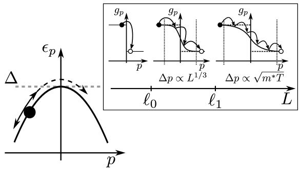
Figure 3: A hole in the vicinity of the bottom of the band with dispersion Eq. (5) performs a random walk in momentum space. In the process of equilibration the holes reverses its direction. The backscattering occurs in a sequence of collisions with excitations at the Fermi level, in which a small relative momentum $\delta p/p_{0}\ll 1$ is transferred to the hole. Inset: Evolution of the hole-distribution at small momenta as the wire length is increased. In the quasi-ballistic regime of relatively short wires $L\lesssim\ell_{0}$ a hole close to the band bottom suffers on average less than one collision when traversing the wire. The voltage induced jump at $p=0$ in this regime is not affected by backscattering and remains of the order $\sim e^{-\Delta/T}eV/T$. Once $L\gg\ell_{0}$ such hole typically experiences many collisions during its passage through the wire which turn its motion in momentum space diffusive. For wires in the inhomogeneous diffusive regime, $\ell_{0}\ll L\ll\ell_{1}$, holes then redistribute in a momentum range scaling with the length of the wire as $\Delta p\propto L^{1/3}$. Only upon entering the homogeneous diffusive regime, $L\gg\ell_{1}$, this range saturates at a momentum-scale set by temperature $\Delta p\sim\sqrt{m^{*}T}$, implying that the hole-distribution becomes a smooth function on this scale.

IV Inhomogeneous diffusive regime

To quantify the above qualitative considerations let us return to Kramers equation (8) and restrict to short wires $\ell_{0}\ll L\ll\ell_{1}$ in the diffusive regime and small momenta, specified momentarily. We then observe that in this inhomogeneous diffusive regime the Fokker-Planck operator is dominated by the second derivative ‘smearing’-operator, and thus a simplified analysis applies where drift is neglected,

$$\frac{p}{m^{*}}\partial_{x}g_{p,x}=\frac{B}{2}\partial^{2}_{p}g_{p,x}\,.$$ (12)

Indeed, if the discontinuity of the hole distribution occurs on a scale $\Delta p\ll\sqrt{m^{*}T}$ in momentum space one may estimate $\partial_{p}g\sim g/\Delta p$. Neglecting drift then amounts to dropping contributions $p\Delta p/m^{*}T\ll 1$ much smaller than unity for small momenta $p\sim\Delta p$ of interest. remark2

It is convenient to define the length scale $\ell_{1}=\sqrt{8m^{*}T^{3}}/B$ and to introduce the dimensionless variables,

$$q={p\over\sqrt{2m^{*}T}},\qquad y={x\over\ell_{1}},\qquad\Lambda={L\over 2\ell_{1}},$$ (13)

in terms of which Eq. (12) takes the form

$$\left(\partial_{q}^{2}-2q\partial_{y}\right)g_{q,y}=0.$$ (14)

Let us now insert the separation ansatz

$$g_{q,y}=\int_{-\infty}^{\infty}da\,b(a)e^{ay}\varphi_{a,q}\,,$$ (15)

where the functions $\varphi_{a,q}$ satisfy the differential equation

$$\left(\partial_{q}^{2}-2qa\right)\varphi_{a}(q)=0.$$ (16)

Then solutions of Eq. (14) in the linear response regime assume the form

$$g_{q,y}=\int_{0}^{\infty}da\,b(a)\left(e^{ay}\varphi_{a}(q)-e^{-ay}\varphi_{a}(-q)\right)\,,$$ (17)

where

$$\varphi_{a}(q)=(2a)^{-2/3}{\rm Ai}((2a)^{1/3}q)$$ (18)

and ${\rm Ai}(x)$ the Airy function. In obtaining Eq. (17) we took advantage of the fact that in the linear response regime the distribution in the center of the wire $g_{q,0}$ is antisymmetric in $q$. Finally, coefficients $b(a)$ are fixed by imposing the boundary conditions,

$$\theta(q)g_{q,-\Lambda}+\theta(-q)g_{q,\Lambda}=-e^{-\Delta/T}\frac{eV}{2T}\operatorname{sgn}(q).$$ (19)

For a detailed discussion on this procedure we refer to Appendix B and move on to the physical implications of our solution.

Our result for the backscattering rate at $\ell_{0}\ll L\ll\ell_{1}$ has the form

$$\dot{N}^{R} =-\zeta{2eV\over h}\left(\frac{L}{\ell_{1}}\right)^{2/3}e^{-\Delta/T},$$ (20)

where $\zeta$ is a numerical coefficient defined through an integral equation and numerically found to be $\zeta\approx 1.25$, as discussed in Appendix B. The resulting power-law dependence $\delta G\propto L^{2/3}$ in the wire length $L$ is a consequence of the scaling form of the Kramers equation and can be understood as follows. peq

In combination with Eq. (10) the power-law scaling $\dot{N}^{R}\propto L^{2/3}$ implies that the discontinuity at $p=0$ in the distribution of right-moving excitations broadens with the distance $x$ from the left lead as $\partial_{p}g_{p,x}|_{p\searrow 0}\sim g/\Delta p\sim x^{-1/3}$. This scaling (and correspondingly for distribution of left-moving excitations with distance from the right lead) reflects the diffusive nature of the backscattering processes. Excitations entering e.g. from the right lead with momentum $\Delta p$, move to the left, gradually decrease their velocity in collisions, and eventually return to the right lead. In order to lose momentum of order $\Delta p$ an excitation has to experience sufficiently many collisions in the wire, which requires a time $t$ determined from the standard diffusion condition $(\Delta p)^{2}\sim Bt$. Propagating through the wire at a typical velocity $\Delta p/m^{*}$ until the turning point, the excitation thus moves a distance $(\Delta p/m^{*})t\sim x$ from the lead. Combining these two observations, one obtains $\Delta p\sim(Bm^{*}x)^{1/3}$, and thus $\dot{N}^{R}\propto\int dx(g/\Delta p)\propto L^{2/3}$.

Finally, let us address the crossover from the inhomogeneous diffusive to the quasi-ballistic regime. The latter is characterized by a length of the wire shorter than the average length scale on which a hole at the bottom of the band scatters off low-energy excitations. This regime recently has been studied by Lunde et al.Lunde2007 for weakly interacting electrons within a perturbative treatment of the Boltzmann equation. This approach builds on the observation that, as the typical highly excited hole participates in at most one collision, backscattering occurs via a single collision and smearing of the hole distribution near $p=0$ can be neglected. Of course, in this regime the picture of diffusive dynamics in momentum space underlying the Fokker Planck approximation does not apply.

To elaborate this point let us recall that the Fokker-Planck approximation relies on a gradient expansion of the collision integral. The latter applies if the typical momentum exchange $q\sim T/v$ in a collision is small compared to the momentum scale $\Delta p\sim(Bm^{*}x)^{1/3}$ on which the distribution varies. Applying this criterion, we find that the inhomogeneous diffusive regime is limited to length scales larger than $\ell_{0}\sim T^{3}/(v^{3}Bm^{*})$. Notice that $\ell_{0}\sim\ell_{1}(T/m^{*}v^{2})^{3/2}$ and at low temperatures $T\ll m^{*}v^{2}$ the result (20) for the inhomogeneous diffusive regime thus applies within a broad region. At the crossover $L\sim\ell_{0}$ the characteristic scale $(L/\ell_{1})^{2/3}\sim T/(m^{*}v^{2})$, and the backscattering rate

$$\dot{N}^{R}\sim-{eV\over h}{T\over m^{*}v^{2}}e^{-\Delta/T}$$ (21)

is thus independent of $B$.

For weak interactions $\ell_{1}$ has been calculated from a microscopic theory. It was shown to be related to the typical time scale for a three-particle collision $\tau_{eee}$ as $\ell_{1}\sim(\mu/T)^{1/2}v_{F}\tau_{eee}$. peq Building on this result we find that at weak interactions the limit of the inhomogeneous diffusive regime is set by $\ell_{0}\sim(T/p_{F})\tau_{eee}$. Notice that $T/p_{F}$ is the velocity of a hole which can backscatter in a single three-particle collision with typical momentum exchange $q\sim T/v_{F}$. We thus observe that in wires of length $L\lesssim\ell_{0}$ such hole will typically suffer at most one collision when traversing the wire, i.e. $L\sim\ell_{0}$ also defines the limit below which the quasi-ballistic regime of Lunde et al.Lunde2007 applies. We thus expect that for $L\lesssim\ell_{0}$ the perturbative calculation of Lunde et al. holds. Indeed, their result $\dot{N}^{R}\sim-{eV\over h}{T\over\mu}{L\over\ell_{0}}e^{-\mu/T}$ at $L\sim\ell_{0}$ matches Eq. (21). The linear scaling $\dot{N}^{R}\propto L$ here simply reflects the fact that in the quasi-ballistic regime the probability of backscattering linearly increases with the time spent in the wire. As this linear dependence does not rely on the assumption of weak interactions, one can use Eq. (21) to extend the result by Lunde et al. to arbitrary interaction strength,

$$\dot{N}^{R}\sim-{eV\over h}{T\over m^{*}v^{2}}{L\over\ell_{0}}e^{-\Delta/T}.$$ (22)

Precise determination of the numerical prefactor in Eq. (22) would require a more careful treatment.

V Crossover to homogeneous diffusive regime

We next discuss how the result for the inhomogeneous diffusive regime $\ell_{0}\ll L\ll\ell_{1}$ crosses over into the homogeneous diffusive regime $\ell_{1}\ll L\ll\ell_{\rm eq}$. To this end we need to address the full inhomogeneous Fokker-Planck equation (8) subject to the boundary conditions (9).

Following the procedure of the previous section we decompose the hole-distribution $g_{p,x}$ into a spatially homogeneous and an inhomogeneous part

$$g_{p,x}=g^{0}_{p}+\delta g_{p,x},$$ (23)

where the homogeneous part is readily found as peq

$$g^{0}_{p}=e^{\epsilon_{p}/T}\left[1-\frac{eV}{\sqrt{2\pi m^{*}T^{3}}}\int^{p}_{0}dp^{\prime}\,e^{-\epsilon_{p^{\prime}}/T}\right]e^{-\Delta/T}\,.$$ (24)

The homogeneous distribution (24) gives a contribution to the backscattering rate (10) that scales linearly with the length of the wire and dominates at $L\gg\ell_{1}$.

To find the inhomogeneous solution we return to the dimensionless variables $q$ and $y$ in Eq. (13) and start out from the ansatz

$$\delta g_{q,y} =e^{a(y-q)}h(q).$$ (25)

This leads us to the differential equation for $h$

$$\partial^{2}_{q}h-2(q+a)\partial_{q}h+2\left(-1+\frac{a^{2}}{2}\right)h=0,$$ (26)

which for the special values of the parameter, $a_{n}=\pm\sqrt{2(n+1)}$ and $n=0,1,...$ is solved by Hermite polynomials with shifted arguments $H_{n}(q\pm a_{n})$. Using again that in the linear response regime $\delta g_{q,y=0}$ is antisymmetric in $q$ and noting that $H_{n}(q)=(-1)^{n}H_{n}(-q)$, the general solution to (8) reads

$$\delta g_{q,y} =\sum_{n=0}^{\infty}b_{n}\left(e^{a_{n}y}\psi_{n}(q)-e^{-a_{n}y}\psi_{n}(-q)\right),$$ (27)

where

$$\psi_{n}(q) =\frac{1}{\sqrt{\mathcal{N}_{n}}}e^{-a_{n}q}H_{n}(q+a_{n}),$$ (28)

and we introduced the normalization constant $\mathcal{N}_{n}=\sqrt{\pi}a_{n}2^{n}n!e^{2(n+1)}$. Expansion coefficients $b_{n}$ are found from matching ansatz (27) to the boundary conditions,

$$\theta(q)g_{q,-\Lambda}+\theta(-q)g_{q,\Lambda} =-{eV\over 2T}e^{q^{2}-\Delta/T}(\operatorname{sgn}(q)-\operatorname{erf}(q)),$$ (29)

and details of this calculation can be found in Appendix C. Accounting then for homogeneous and inhomogeneous contributions to the distribution function the backscattering rate reads

$$\dot{N}^{R}=-{2eV\over h}\left(\frac{L}{\sqrt{\pi}\ell_{1}}+I^{t}\left(\openone+OX\right)^{-1}XI\right)e^{-\Delta/T}\,,$$ (30)

where we introduced vector $I$ and matrices $X$, $O$, respectively, with coefficients

$$I_{m} =-\psi^{\prime}_{m}(0)/a_{m},$$ (31)

$$X_{mn} =\delta_{mn}\left(1-e^{-2a_{n}\Lambda}\right)/2,$$ (32)

$$O_{mn} =\begin{cases}c_{mm}+\int_{0}^{\infty}dp^{2}\,e^{-p^{2}-a_{m}^{2}}\psi^{2}_{m}(p),\quad m=n\\ {2\over a^{2}_{m}-a^{2}_{n}}\left(a_{m}^{2}c_{mn}-a_{n}^{2}c_{nm}\right),\quad m\neq n\end{cases}$$ (33)

and $c_{mn}=I_{m}\psi_{n}(0)$.

In the inhomogeneous diffusive regime $\ell_{0}\ll L\ll\ell_{1}$ main contributions to Eq. (30) originate from coefficients with large index $n\gg\ell_{1}/L$. This allows to approximate Hermite polynomials in the eigenfunctions (28) by Airy functions according to Dominici2006 $H_{n}(z)\simeq\sqrt{2\pi(2n)^{n}}n^{1/6}\mathrm{Ai}\left(\sqrt{2}n^{1/6}(x-\sqrt{2n})\right)e^{-\frac{3}{2}n+\sqrt{2n}z}$. Reassuringly, upon this substitution one recovers Eq. (20).

In the opposite limit $L\gg\ell_{1}$ one may approximate $2X\simeq\openone$ and thus finds the backscattering rate

$$\dot{N}^{R}=-{2eV\over h}\left({L\over\sqrt{\pi}\ell_{1}}+\xi\right)e^{-\Delta/T},$$ (34)

with an universal offset numerically calculated as $\xi\simeq 0.275$.

To address the crossover regime at arbitrary ratios $L/\ell_{1}$ we numerically evaluated (30). The resulting backscattering rate leads to a finite temperature correction to the conductance (1) shown in Fig. 4. We observe that the characteristic power-law $\dot{N}^{R}\propto L^{2/3}$ of the inhomogeneous diffusive regime extends up to lengths of the wire $L\lesssim 0.4\ell_{1}$. Once the wire length exceeds $L\gtrsim 0.8\ell_{1}$, the correction follows the linear length dependence of the homogeneous diffusive regime with the universal off-set $\xi\simeq 0.275$. These features hold for weak as well as strong interaction, and the peculiar power law dependence of $\delta G$ on the wire length is, therefore, characteristic to short clean quantum wires $\ell_{0}\ll L\ll\ell_{\rm eq}$.

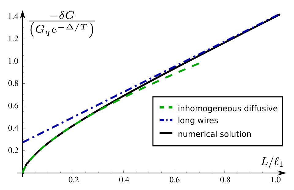
Figure 4: Length dependence of the interaction-induced correction to the conductance Eq. (1), found from the backscattering rate of quantum wires $\ell_{0}\ll L\ll\ell_{\rm eq}$. Solid line shows the result obtained from numerically solving Eqs. (30)-(33). Asymptotic results for wires much shorter and much longer than $\ell_{1}$, Eqs. (20) and (34) respectively, are indicated by dashed and dash-dotted lines. The characteristic scaling $\delta G\propto L^{2/3}$ in the inhomogeneous diffusive regime holds up to $L\lesssim 0.4\ell_{1}$, and then crosses over to the result for the homogeneous diffusive regime with its linear length dependence and universal off-set $\xi\simeq 0.275$.

VI Summary and discussion

We have studied the interaction-induced backscattering rate $\dot{N}^{R}$ in a voltage-biased clean quantum wire, in which conservation laws suppress relaxation. Our calculations apply for wires in a broad range of lengths $\ell_{0}\ll L\ll\ell_{\rm eq}\propto e^{\Delta/T}$, which are short in the sense that equilibration has not fully established, but long enough to guarantee diffusive motion in momentum space due to interaction-induced collisions. In these wires, a finite rate $\dot{N}^{R}$ arises due to the backscattering of mobile holes at the band bottom performing the random motion of a Brownian particle in momentum space while scattering from excitations at the Fermi level. Reminiscent to the first passage problem the dynamics of the hole is described by an inhomogeneous Fokker-Planck equation.

From solutions of the latter we have derived the wire length dependence of the interaction-induced correction to the conductance (1), and found a power law scaling $\delta G\propto L^{2/3}$ as a characteristic feature of these wires. We have identified the length scale $\ell_{0}$ which separates the diffusive from the quasi-ballistic regime. The latter has previously been studied by Lunde et al. Lunde2007 in the limit of weak interactions. We confirmed that for weakly interacting electrons backscattering rates in both regimes match at the crossover scale $L\sim\ell_{0}$, and were able to generalize the results by Lunde et al. to arbitrary interaction strengths.

Our results hold for weakly as well as strongly interacting electrons. They depend on the interaction strength via the bandwidth of excitations $\Delta$, which sets the activation energy $e^{-\Delta/T}$, and effective mass $m^{*}$ and diffusion constant $B$, which both define the relevant length scale of the problem, $\ell_{1}$. The activation behavior $e^{-\Delta/T}$ dominates the temperature dependence of the backscattering rate and corresponding correction to the conductance. An additional temperature dependence enters via the diffusion constant defining the pre-exponential factor. The diffusion constant has been studied for spin-polarized electrons at arbitrary interactions peq ; eqWC ; eqLL ; Matveev2012 where a temperature dependence $B\sim T^{5}$ was found. While a generalization accounting for spin degree of freedom and applicable at arbitrary interaction strength is still an open problem, the strongly interacting limit of a Wigner crystal has been addressed recently. MatveevAndreevKlironomos There, a scaling $B\sim T^{3}$ was found, and a similar result holds at arbitrary interaction strength. to be published

Acknowledgments

K. A. M. and T. M. acknowledge fruitful discussions with J. Rech. Work by M. T. R. was supported by the Alexander von Humboldt Foundation. T. M. acknowledges support by Brazilian agencies CNPq and FAPERJ. Work by K. A. M. was supported by the U.S. Department of Energy, Office of Science, Materials Sciences and Engineering Division. A. L. acknowledges support from NSF grant DMR-1401908 and GIF, and thanks I. V. Gornyi and D. G. Polyakov for numerous important discussions.

Appendix A Orthogonality relations

The inhomogeneous solution to the FPE (8) is expanded in functions $\psi_{n}(\pm q)$ which are eigenfunctions of the differential operator

$$\mathcal{D}={1\over q}\partial_{q}\left({1\over 2}\partial_{q}-q\right),$$ (35)

i.e. $\mathcal{D}\psi_{m}(sq)=sa_{m}\psi_{m}(sq)$, with $s=\pm$, and are orthogonal with respect to a weight function $w(q)$ to be determined in the following way. From the eigenvalue problem it follows that

$$\psi_{n}(sq)\mathcal{D}\psi_{m}(s^{\prime}q)-\psi_{m}(s^{\prime}q)\mathcal{D}\psi_{n}(sq)$$

$$\qquad=\left(s^{\prime}a_{m}-sa_{n}\right)\psi_{n}(sq)\psi_{m}(s^{\prime}q),\quad s,s^{\prime}=\pm.$$ (36)

Multiplying both sides with a, yet to be determined, function $w(q)$, integrating over the entire momentum range and imposing an orthogonality condition

$$\int_{-\infty}^{\infty}dq\,w(q)\psi_{n}(sq)\psi_{m}(s^{\prime}q) =-s\delta_{ss^{\prime}}\delta_{n,m},$$ (37)

we find the weight function to be determined by the differential equation

$$-{1\over 2q}\partial_{q}w(q)+w(q)\left({1\over 2q^{2}}-1\right)=0,$$ (38)

resulting in $w(q)=qe^{-q^{2}}$.

In the inhomogeneous diffusive regime the differential operator of interest reads

$$\mathcal{D} ={1\over 2q}\partial^{2}_{q},$$ (39)

and following the same steps as above one arrives at the orthogonality relation for Airy-functions

$$\int_{-\infty}^{\infty}dq\,q{\rm Ai}(\alpha q){\rm Ai}(\beta q)=-{1\over 3\alpha}\delta(\alpha-\beta).$$ (40)

Appendix B Details on the inhomogeneous diffusive regime

We give details on the derivation of the expansion coefficients defining the hole distribution function in (15) and the backscattering rate in the inhomogeneous diffusive regime.

Coefficients $b(a)$ are found from matching (17) to the boundary condition

$$\theta(q)g_{q,-\Lambda}+\theta(-q)g_{q,\Lambda} =-e^{-\Delta/T}\frac{eV}{2T}\operatorname{sgn}(q),$$ (41)

Inserting the explicit form of the general solution $g_{q,y}$ and expressing $e^{x}=\cosh x+\sinh x$ one finds

$$\int_{0}^{\infty} da{b(a)\over(2a)^{2/3}}\left[e^{a\Lambda}\operatorname{Ai}((2a)^{1/3}q)-e^{-a\Lambda}\operatorname{Ai}(-(2a)^{1/3}q)\right.$$

$$\left.-2\Theta(q)\sinh(a\Lambda)\left(\operatorname{Ai}((2a)^{1/3}q)+\operatorname{Ai}(-(2a)^{1/3}q)\right)\right]$$

$$=-e^{-\Delta/T}\frac{eV}{2T}\operatorname{sgn}(q).$$ (42)

Coefficients $b(a)$ can then be extracted using the orthogonality relation for Airy-functions (40), i.e. by multiplying left and right hand side of (B) with ‘$q\operatorname{Ai}\left((2a_{0})^{1/3}q\right)$’ where $a_{0}>0$ and integrating over all $q$. For the right hand side of (B) we may further use that

$$\int_{-\infty}^{\infty}dq\,|q|\operatorname{Ai}\left((2a_{0})^{1/3}q\right) =-2^{1/3}a_{0}^{-2/3}\operatorname{Ai}^{\prime}(0)$$ (43)

where we used the defining differential equation for Airy functions, to e.g. calculate $\alpha^{3}\int_{0}^{\infty}dq\,q\operatorname{Ai}(\alpha q)=\int_{0}^{\infty}dq\,\partial_{q}^{2}\operatorname{Ai}(\alpha q)=-\alpha\operatorname{Ai}^{\prime}(0)$. We then find

$${b(a_{0})e^{a_{0}\Lambda}\over(16a_{0})^{1/3}}+\int_{0}^{\infty}da\,{b(a)\over(2a)^{2/3}}\sinh(a\Lambda){\cal F}(a,a_{0}) =-{2^{1/3}\operatorname{Ai}^{\prime}(0)\over a_{0}^{2/3}}{eV\over 2T}e^{-\Delta/T},$$ (44)

where

$${\cal F}(a,a_{0}) =2\int_{0}^{\infty}dq\,q\operatorname{Ai}((2a_{0})^{1/3}q)\left(\operatorname{Ai}\left((2a)^{1/3}q\right)+\operatorname{Ai}\left(-(2a)^{1/3}q\right)\right).$$ (45)

The function ${\cal F}$ can be further calculated with help of the identity

$$\left[2a-s2a_{0}\right]\int_{0}^{\infty}dq\,q\operatorname{Ai}\left((2a)^{1/3}q\right)\operatorname{Ai}\left(s(2a_{0})^{1/3}q\right)$$

$$\qquad=-\left[(2a)^{1/3}-s(2a_{0})^{1/3}\right]\operatorname{Ai}^{\prime}(0)\operatorname{Ai}(0),$$ (46)

which again results from using the defining differential equation for the Airy function to express $q\operatorname{Ai}(\alpha q)=\alpha^{-3}\partial_{q}^{2}\operatorname{Ai}(\alpha q)$, and gives

$${\cal F}(a,a_{0}) =-\operatorname{Ai}^{\prime}(0)\operatorname{Ai}(0){(2a)^{4/3}-(2a_{0})^{4/3}\over a^{2}-a_{0}^{2}}.$$ (47)

We thus find from orthogonal projection the integral equation

$$\beta(a_{0}\Lambda)+{a_{0}^{2/3}\over\sqrt{3}\pi}\int_{0}^{\infty}{da\over a}\beta(a\Lambda)\left(1-e^{-a\Lambda}\right){a_{0}^{4/3}-a^{4/3}\over a_{0}^{2}-a^{2}}=1,$$ (48)

where we introduced

$$b(a) =-{2^{2/3}{\rm Ai}^{\prime}(0)\over a^{1/3}}{eV\over T}e^{-\Delta/T}e^{-a\Lambda}\beta(2a\Lambda),$$ (49)

and employed that $\operatorname{Ai}^{\prime}(0)\operatorname{Ai}(0)=-\left(2\sqrt{3}\pi\right)^{-1}$. Rescaling $a$ and $a_{0}$ by the factor $1/\Lambda$ one arrives at the expression stated in the main text.

Finally, the backscattering rate expressed in dimensionless variables

$$\dot{N}^{R} ={2T\over h}\int_{-\Lambda}^{\Lambda}dy\,\left(\partial_{q}g_{q,y}\right)|_{q=0}$$ (50)

is readily calculated as

$$\dot{N}^{R} =2^{8/3}\operatorname{Ai}^{\prime}(0){T\over h}\int_{0}^{\infty}{da\over a^{4/3}}b(a)\sinh(a\Lambda),$$ (51)

or expressed in terms of $\beta(a)$ (see Eq. (49))

$$\dot{N}^{R} =-\left(2\operatorname{Ai}^{\prime}(0)\right)^{2}{2eV\over h}e^{-\Delta/T}\int_{0}^{\infty}{da\over a^{5/3}}\beta(a\Lambda)\left(1-e^{-a\Lambda}\right).$$ (52)

We may now scale $\Lambda$ out of the integral and find the result Eq. (20) stated in the main text, with a numerical constant $\zeta={(4/3)^{2/3}\over\Gamma^{2}(1/3)}\int_{0}^{\infty}da{\beta(a)\over a^{5/3}}\left(1-e^{-a}\right)$, where the latter involves a solution of the integral equation,

$$\beta(a_{0})+\gamma a_{0}^{2/3}\int_{0}^{\infty}{da\over a}\left(1-e^{-a}\right){a^{4/3}-a_{0}^{4/3}\over a^{2}-a_{0}^{2}}\beta(a)=1,$$ (53)

and $\gamma=1/\sqrt{3}\pi$. Solving (53) numerically we find $\zeta~{}\simeq~{}1.25$.

Appendix C Details on the crossover regime

We give details on the derivation of the expansion coefficients defining the hole distribution function and the backscattering rate in the crossover regime.

Coefficients $b_{n}$ entering the general solution (27) are derived from the boundary conditions discussed in the main text in a similar way as discussed in the previous section. Employing the orthogonality relation (37) for the general eigenfunctions and proceeding analogously as in the inhomogeneous diffusive regime we arrive at the following equation, generalizing (48) to the crossover regime,

$$\beta_{n}+{1\over 2}\sum_{m=0}^{\infty}O_{nm}\left(1-e^{-2a_{n}\Lambda}\right)\beta_{m} =I_{n}.$$ (54)

Here we introduced (similar to (49))

$$b_{n}={eV\over 2T}e^{-\Delta/T}e^{-a_{n}\Lambda}\beta_{n},$$ (55)

and vector and matrix elements $I_{m}$ and $O_{mn}$, respectively, are defined as

$$I_{n} =\int_{-\infty}^{\infty}dq\,q\psi_{m}(q)\left(\operatorname{sgn}(q)-\operatorname{erf}(q)\right),$$ (56)

$$O_{mn} =2\int_{0}^{\infty}dq\,qe^{-q^{2}}\psi_{m}(q)\left(\psi_{n}(q)+\psi_{n}(-q)\right).$$ (57)

The above integrals can be evaluated using eigenvalue equations below (35). We may express vector elements e.g. as

$$I_{m} ={1\over a_{m}}\int_{-\infty}^{\infty}dq\,\mathcal{L}\psi_{m}(sq)\left(\operatorname{sgn}(q)-\operatorname{erf}(q)\right),$$ (58)

with $\mathcal{L}=q\mathcal{D}$ and ${\cal D}$ from Eq. (35), and upon integration by parts (notice that boundary terms vanish) find

$$I_{m}=-{1\over a_{m}} \Big{[}\left(\partial_{q}\psi_{m}(q)-2q\psi_{m}(q)\right)|_{q=0}$$

$$-\int_{-\infty}^{\infty}{dq\over\sqrt{\pi}}\partial_{q}\left(e^{-q^{2}}\psi_{m}(q)\right)\Big{]},$$ (59)

as stated in the main text.

In a similar way we calculate integrals defining matrix elements $O_{mn}$ starting out from

$$\int_{0}^{\infty}dq\,qe^{-q^{2}}\psi_{m}(q)\psi_{n}(sq) ={1\over a_{m}}\int_{0}^{\infty}dq\,e^{-q^{2}}\mathcal{L}\psi_{m}(q)\psi_{n}(sq).$$ (60)

Upon partial integration and further algebraic manipulations we arrive at

$$2\int_{0}^{\infty}dq\,qe^{-q^{2}}\psi_{m}(q)\psi_{n}(sq)$$

$$\qquad={1\over a_{m}-sa_{n}}\left(s\psi_{m}(0)\psi^{\prime}_{n}(0)-\psi_{n}(0)\psi^{\prime}_{m}(0)\right),$$ (61)

which applies for all $m$, $n$ ($m\neq n$) if $s=-$ ($s=+$), and leads to the result stated in the main text.

Finally, the backscattering rate is found from the general expression,

$$\dot{N}^{R} ={8T\over h}\sum_{n}{b_{n}\over a_{n}}\psi_{n}^{\prime}(0)\sinh(a_{n}\Lambda),$$ (62)

upon introducing $I_{n}=\psi^{\prime}(0)/a_{n}$ and inserting the formal solution to Eq. (54),

$$\beta_{n} =\sum_{m}\left((1+OX)^{-1}\right)_{nm}I_{m},$$ (63)

with $\beta_{n}$ defined in Eq. (55).

References

- (1) A. Polkovnikov, K. Sengupta, A. Silva, and M. Vengalattore, Rev. Mod. Phys. 83, 863 (2011).
- (2) A. Imambekov, T. L. Schmidt, and L. I. Glazman, Rev. Mod. Phys 84, 1253, (2012).
- (3) T. Kinoshita, T. Wenger and D. S. Weiss, Nature 440, 900 (2006).
- (4) G. Barak, H. Steinberg, L. N. Pfeiffer, K. W. West, L. I. Glazman, F. von Oppen, and A. Yacoby, Nature Phys. 6, 489 (2010).
- (5) J. Rech, T. Micklitz, and K. A. Matveev, Phys. Rev. Lett. 102, 116402 (2009).
- (6) T. Micklitz, J. Rech, and K. A. Matveev, Phys. Rev. B 81, 115313 (2010).
- (7) K. A. Matveev and A. V. Andreev, Phys. Rev. B 85, 041102(R) (2012).
- (8) K. A. Matveev and A. V. Andreev, Phys. Rev. Lett. 107, 056402 (2011).
- (9) K. A. Matveev, A. V. Andreev, and M. Pustilnik, Phys. Rev. Lett. 105, 046401 (2010).
- (10) A. M. Lunde, K. Flensberg, and L. I. Glazman, Phys. Rev. B 75, 245418 (2007).
- (11) A. Levchenko, Z. Ristivojevic, and T. Micklitz, Phys. Rev. B 83, 041303(R) (2011).
- (12) A. H. Castro Neto and M. P. A. Fisher, Phys. Rev. B 53, 9713 (1996).
- (13) D. L. Maslov and M. Stone, Phys. Rev. B 52, R5539 (1995).
- (14) V. V. Ponomarenko, Phys. Rev. B 52, R8666 (1995).
- (15) I. Safi and H. J. Schulz, Phys. Rev. B 52, R17040 (1995).
- (16) K. A. Matveev, JETP 117, 508 (2013).
- (17) H. A. Kramers, Physica 7, 284 (1940).
- (18) H. Risken, The Fokker-Planck Equation: Methods of Solution and Applications, Springer Series (1996).
- (19) K. A. Matveev, A. V. Andreev, and A. D. Klironomos, Phys. Rev. B 90, 035148 (2014).
- (20) K. A. Matveev and A. V. Andreev, Phys. Rev. B 86, 045136 (2012).
- (21) Nonequilibrium corrections to Fokker-Planck equation (8) affecting states near the Fermi points have been derived and analyzed in the context of Coulomb drag problem, see Ref. DGP, for extensive details.
- (22) A. P. Dmitriev, I. V. Gornyi, and D. G. Polyakov, Phys. Rev. B 86, 245402 (2012).
- (23) D. Dominici, JDEA 13, 1115 (2007).
- (24) M. T. Rieder, A. Levchenko, and T. Micklitz, in preparation.