A Novel Spectrally-Efficient Scheme for Physical Layer Network Coding

Abstract

In this paper, we propose a novel three-time-slot transmission scheme combined with an efficient embedded linear channel equalization (ELCE) technique for the Physical layer Network Coding (PNC). Our transmission scheme, we achieve about $33\%$ increase in the spectral efficiency over the conventional two-time-slot scheme while maintaining the same end-to-end BER performance. We derive an exact expression for the end-to-end BER of the proposed three-time-slot transmission scheme combined with the proposed ELCE technique for BPSK transmission. Numerical results demonstrate that the exact expression for the end-to-end BER is consistent with the BER simulation results.

I Introduction

Network Coding (PNC) is a relatively new paradigm in networking which is based on exploiting interference, instead of avoiding it, to significantly enhance network throughput, robustness, and security [1]. It has been extensively studied for wired networks and wireless ad-hoc networks [2, 3]. The concept of physical-layer network coding (PNC) was originally proposed in [4] as a way to exploit network coding operation [5, 6] that occurs naturally in superimposed electromagnetic (EM) waves. The laws of physics show that when multiple EM waves come together within the same physical space, they mix. This mixing of EM waves is a form of network coding, performed by nature. Using PNC in a Two-Way Relay Channel (TWRC) boosts the system throughput by 100% [4].

Fig. 1 illustrates the idea of the concept of network coding. In the first time slot, nodes 1 and 2 transmit $S_{1}$ and $S_{2}$ simultaneously to relay R. Relay R deduces $S_{R}$= $S_{1}\oplus S_{2}$ . Then, in the second time slot, relay R broadcasts $S_{R}$ to nodes 1 and 2, where $\oplus$ refers to the XOR operation.

The main issue in PNC is how relay R deduces $S_{R}$= $S_{1}\oplus S_{2}$ from the superimposed EM waves, which is referred as “PNC mapping”. Generally, PNC mapping is the process of mapping the received mixed EM waves plus noise to the desired-network coded signal for forwarding by the relay to the two end nodes. In general, PNC mapping in not restricted to the XOR mapping.

In [7], the authors investigate the Symbol Error Rate (SER) performance for BPSK and QPSK schemes for two end nodes with in-phase and orthogonal constellation in AWGN environment. The analysis assumes perfect channel estimation and takes into consideration the effect of power control at the two end nodes. The authors use the Craig’s polar coordinate algorithm [8] to derive an exact expression for the SER.

Most of the work found in literature assumes that the two received streams which compose the superimposed EM wave at the relay can be perfectly resolved and channel-equalized using channel estimates at the relay based on channel estimation techniques presented in the literature, such as [9, 10, 11]. Practically, such resolvability assumption contradicts the main principle of PNC operation which relies on utilizing the natural superposition of EM waves from both end nodes at the relay to map these signals into the desired-network coded signal to be forwarded by the relay to the two end nodes without the separation at the relay.

In this paper, we propose an efficient embedded linear channel equalization (ELCE) technique to perfectly equalize the channels without resolving data streams from each node using a three-time-slot system assuming perfect channel estimation at the relay node. In addition to overcoming the impractical assumption of stream separation, our proposed three-time-slot scheme achieves about $33\%$ increase in spectral efficiency compared to the BPSK transmission presented in [4] while maintaining the same BER performance of resolvable BPSK and QPSK PNC schemes. The achieved spectral efficiency lies between the one of BPSK assuming resolvable streams at the relay node and QPSK assuming resolvable nodes’ beams at relay. Finally, we present an exact analysis for the end-to-end bit-error rate (BER) expression for the proposed three-time-slot scheme assuming BPSK transmission under Rayleigh fading channel.

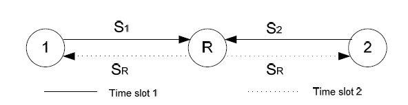
Figure 1: Physical Layer Network Coding approach (PNC) [4]

The rest of this paper is organized as follows: In Section II, we describe our three-time-slot system model. Section III presents our proposed ELCE technique. An exact end-to-end BER expression for the proposed three-time-slot scheme over the Rayleigh fading channels is derived in Section IV. In Section V, we provide the numerical results for the proposed three-time-slot scheme combined with the ELCE technique and we conclude the paper in Section VI.

II System Model

In this section, we introduce our system model tailored with our proposed three-time-slot scheme for a communication system using PNC for TWRC. The relay and the users are assumed fully symbol-synchronized. Channels are assumed to be Rayleigh fading with channel gains represented as circulary symmetric complex random variables and the noise is Additive White Gaussian (AWGN) with zero mean. We also assume that all the channels’ state information are available at the receivers side. As illustrated in Fig. 2, node $1$ and node $2$ send two successive symbols with $90^{o}$ phase difference between them, $i.e.$ node 1 and node 2 will send $(S_{11}+jS_{12})$ and $(S_{21}+jS_{22})$, respectively, to the relay node in the first time slot, where $S_{11},\,S_{12}$ and $S_{21},\,S_{22}$ are two successive symbols of node 1 and node 2, respectively. Then, in the second time slot, node 2 repeats its transmission of $(S_{21}+jS_{22})$, however, node 1 retransmits a $90^{o}-shifted$ version of its transmission in the first slot, $i.e.$ it transmits $j(S_{11}+jS_{12})$. The relay node adopts the ELCE technique, described in Section III, followed by a PNC mapping using the superimposed EM waves $Y_{1}$ and $Y_{2}$ received at the relay node in the first two time slots. In the third slot, the relay transmits the PNC-mapped data $S_{R}$ to the end nodes. Hence, we transmit four symbols in three time slots which means a $33\%$ spectral efficiency increase over the conventional two-slot scheme in [4]. The two superimposed EM waves $Y_{1}$ and $Y_{2}$ can be expressed as follows

$$Y_{1} =h_{1}(S_{11}+jS_{12})+h_{2}(S_{21}+jS_{22})+n_{1}$$ (1)

$$Y_{2} =jh_{1}(S_{11}+jS_{12})+h_{2}(S_{21}+jS_{22})+n_{2},$$ (2)

where $h_{1}$, $h_{2},$ $n_{1}$, and $n_{2}$ are the channel between node 1 and the relay, the channel between node 2 and the relay, the noise at the relay receiver at the first time slot with variance $\sigma_{1}^{2}$, and the noise at the relay receiver at the second time slot with variance $\sigma_{2}^{2}$, respectively. We assume that $h_{1}$and $h_{2}$ are block fading channels with constant amplitudes during the full transmission time ($i.e.$ during the three time slots). We also assume equal noise variance for $n_{1}$ and $n_{2}$, $i.e.$ $\sigma_{1}^{2}=\sigma_{2}^{2}=\sigma^{2}$.

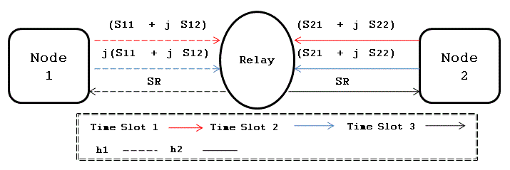
Figure 2: Proposed Three-Time-Slot scheme for a communication system using PNC for TWRC

III Embedded Linear Channel Equalization (ELCE) Technique

In this section, we present the proposed ELCE technique for perfect channel equalization assuming perfect channel estimation at the relay and the end nodes. Starting from Eqs. (1) and (2), we multiply Eqs. (2) and (1) by $\frac{h_{1}^{*}}{\left\|h_{1}\right\|^{2}}$ and $\frac{h_{2}^{*}}{\left\|h_{2}\right\|^{2}}$, respectively to produce $Z_{1}$ and $Z_{2}$, respectively. Hence, the received-signal vector $\underline{Z}=\left[\begin{array}[]{c}Z_{1}\\ Z_{2}\end{array}\right]$ can be expressed as follows

$$\underline{Z}=\left[\begin{array}[]{cc}j&\frac{h_{1}^{*}h_{2}}{\left\|h_{1}\right\|^{2}}\\ \frac{h_{1}h_{2}^{*}}{\left\|h_{2}\right\|^{2}}&1\end{array}\right]\left[\begin{array}[]{c}(S_{11}+jS_{12})\\ (S_{21}+jS_{22})\end{array}\right]+\left[\begin{array}[]{c}\frac{h_{1}^{*}}{\left\|h_{1}\right\|^{2}}\,n_{2}\\ \frac{h_{2}^{*}}{\left\|h_{2}\right\|^{2}}\,n_{1}\end{array}\right]$$ (3)

We construct the channel-equalized-signal vector $\underline{X}=\left[\begin{array}[]{c}X_{1}\\ X_{2}\end{array}\right]$ by left multiplying $\underline{Z}$ by the equalization matrix $\mathbf{\underline{H}}$ which is defined as follows

$$\mathbf{\underline{H}}=\mathbf{\frac{1}{2}\mathbf{\left[\vphantom{}\begin{array}[]{cc}\left(1+j\right)&0\\ 0&\left(1-j\right)\end{array}\right]}\left[\vphantom{}\begin{array}[]{cc}\frac{h_{1}h_{2}^{*}}{\left\|h_{2}\right\|^{2}}&-j\\ -j&j\,\frac{h_{1}^{*}h_{2}}{\left\|h_{1}\right\|^{2}}\end{array}\right]}$$ (4)

therefore, $\underline{X}$ can be expressed as follows

$$\underline{X} =\underline{\mathbf{H}\,}\underline{Z}$$

$$=\left[\begin{array}[]{c}(S_{21}+jS_{22})\\ (S_{11}+jS_{12})\end{array}\right]+\frac{1}{2}\left[\begin{array}[]{c}\,\,\frac{(1+j)\,h_{2}^{*}}{\left\|h_{2}\right\|^{2}}\left(n_{1}-jn_{2}\right)\\ -j\frac{(1-j)\,h_{1}^{*}}{\left\|h_{1}\right\|^{2}}\left(n_{1}-n_{2}\right)\end{array}\right]$$ (9)

The relay node calculates the perfectly channel-equalized combined signal $X^{ELCE}=X_{1}+X_{2}$ which is equivalent to the superimposed EM wave at the relay node used to perform the PNC mapping before forwarding to both end nodes. Hence, the signal $X^{ELCE}$ can be expressed as follows

$$X^{ELCE} =\left[\mathbf{S_{2}}+\frac{1}{2}\frac{(1+j)\,h_{2}^{*}}{\left\|h_{2}\right\|^{2}}\left(n_{1}-jn_{2}\right)\right]$$

$$+\left[\mathbf{S_{1}}+\frac{1}{2}\frac{-j(1-j)\,h_{1}^{*}}{\left\|h_{1}\right\|^{2}}\left(n_{1}-n_{2}\right)\right]$$ (10)

where $\mathbf{S_{1}}=(S_{11}+jS_{12})$ and $\mathbf{S_{2}}=(S_{21}+jS_{22})$

IV Exact End-to-End BER Performance for the Proposed Three-Time-Slot Scheme

In this section, we provide the BER performance analysis for the proposed three-time-slot scheme at the relay node for BPSK modulation scheme at each node. Fig. 3 shows the received signal constellation at the relay node assuming that both end nodes use BPSK modulation scheme. We assume that $E_{b_{1}}$ and $E_{b_{2}}$ are the constant bit energy for the BPSK signal generated from nodes 1 and 2, respectively. Then, each node start performing the proposed three-time-slot scheme by combining each two successive BPSK symbols ($i.e.$ $S_{11},\,S_{12}$ and $S_{21},\,S_{22}$ for node 1 and 2, respectively, with $2$ different possibilities ”$0$ and $1$“ for each symbol) together into one QPSK symbol ($i.e.$ $\mathbf{S_{1}}$ and $\mathbf{S_{2}}$ for node 1 and 2, respectively, with $4$ different possibilities ”$00$, $01$, $10$, and $11$” for each symbol) and transmit it to the relay node. Consequently, there are sixteen possible symbols in the combined received signal constellation at the relay node ($i.e.$ for noise-free $X^{ELCE}=\mathbf{S_{1}}+\mathbf{S_{2}}$ ). Then, the relay node performs the PNC mapping on the noise-free $X^{ELCE}$ to construct the QPSK-mapped signal $\mathbf{S_{R}=\mathbf{S_{1}}\oplus\mathbf{S_{2}}}$ and broadcasts it to the end nodes in the third time-slot as shown in Fig. 2. Since, $\mathbf{S_{R}=\mathbf{S_{1}}\oplus\mathbf{S_{2}=(S_{11}+jS_{12})+(S_{21}+jS_{22})}}$ and $S_{11},\,S_{12}$,$S_{21},$ and $S_{22}$ are BPSK symbols, hence, each combined symbol $\mathbf{S_{R}}$ at relay node is resulted by the addition of encoded four bits. However, the relay node maps $\mathbf{S_{R}}$ to a QPSK PNC-mapped signal to broadcast it to the end nodes at the third time-slot. We assume that $E_{b_{1}}\geq E_{b_{2}}$, therefore, we have sixteen decision regions bounded by decision boundaries $\pm E_{b_{1}}$ for in-phase and quadrature components in the signal constellation as shown in Fig. 3.

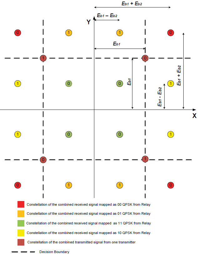
Figure 3: The received constellation at the relay node for BPSK signal for the proposed three-time-slot transmission scheme

To simplify the analysis, we use the Craig’s polar coordinate algorithm [8] for symbol-error rate (SER) calculation for AWGN channels. Furthermore, we extend this analysis for the fading channels by using the instantaneous value of noise variance $\sigma_{N}^{2}\left(|h_{1}|^{2},|h_{2}|^{2}\right)$ which can be proved from Eq. (10) to be as $\sigma_{N}^{2}\left(|h_{1}|^{2},|h_{2}|^{2}\right)=\sigma^{2}\left[\frac{1}{|h_{1}|^{2}}+\frac{1}{|h_{2}|^{2}}\right]$ and we can consider $\sigma_{N}^{2}\left(|h_{1}|^{2},|h_{2}|^{2}\right)$ as the new instantaneous noise variance of a zero mean AWGN signal added to the desired signal $after$ performing the ELCE technique. Although we apply our analysis to BPSK only, however it can be extended to higher modulation.

Let $F_{e/0}\left(|h_{1}|^{2},|h_{2}|^{2}\right)$ denotes the instantaneous probability of symbol error in the PNC mapping process at the relay due to the noise effect assuming that the noise-free PNC-mapped signal is “0” ($i.e.$ $S_{R}=0$), and $F_{e/1}\left(|h_{1}|^{2},|h_{2}|^{2}\right)$ denotes the instantaneous probability of symbol error in the PNC mapping process at the relay due to the noise effect assuming that the noise-free PNC-mapped signal is “1” ($i.e.$ $S_{R}=1$), where $|h_{1}|^{2}$ and $|h_{2}|^{2}$ are the channel gains for $h_{1}$and $h_{2}$, respectively.

Using Craig’s polar coordinate algorithm [8], we develop the instantaneous expressions for $F_{e/0}\left(|h_{1}|^{2},|h_{2}|^{2}\right)$ and $F_{e/1}\left(|h_{1}|^{2},|h_{2}|^{2}\right)$ exploiting the previous definition of $\sigma_{N}^{2}\left(h_{1}|^{2},|h_{2}|^{2}\right)$. To simplify the notation, we denote $\sigma_{N}^{2}=\sigma_{N}^{2}\left(h_{1}|^{2},|h_{2}|^{2}\right)=\sigma^{2}\left[\frac{\gamma_{1}+\gamma_{2}}{\gamma_{1}\gamma_{2}}\right]$, $\gamma_{1}=|h_{1}|^{2}$, $\gamma_{2}=|h_{2}|^{2},$ $F_{e/0}^{inst}\left(\gamma_{1},\gamma_{2}\right)=F_{e/0}\left(|h_{1}|^{2},|h_{2}|^{2}\right)$, and $F_{e/1}^{inst}\left(\gamma_{1},\gamma_{2}\right)=F_{e/1}\left(|h_{1}|^{2},|h_{2}|^{2}\right)$. Consequently, the average probability of symbol error over the fading channel given that symbol “0” was transmitted $P_{e/0}^{Symbol}$ and the average probability of symbol error over the fading channel given that symbol “1” was transmitted $P_{e/1}^{Symbol}$ can be expressed as follows

$$P_{e/0}^{Symbol} =\int_{\gamma_{1}}\int_{\gamma_{2}}F_{e/0}^{inst}\left(\gamma_{1},\gamma_{2}\right)\,f_{\gamma_{1}}(\gamma_{1})f_{\gamma_{2}}(\gamma_{2})d\gamma_{1}d\gamma_{2}$$ (11)

$$P_{e/1}^{Symbol} =\int_{\gamma_{1}}\int_{\gamma_{2}}F_{e/1}^{inst}\left(\gamma_{1},\gamma_{2}\right)\,f_{\gamma_{1}}(\gamma_{1})f_{\gamma_{2}}(\gamma_{2})d\gamma_{1}d\gamma_{2}$$ (12)

where $f_{\gamma_{1}}(\gamma_{1})$ and $f_{\gamma_{2}}(\gamma_{2})$ are the probability density function (PDF) of the channel gains of $\gamma_{1}$ and $\gamma_{2}$, respectively. From [8], we derive $F_{e/0}^{inst}\left(\gamma_{1},\gamma_{2}\right)$ and $F_{e/1}^{inst}\left(\gamma_{1},\gamma_{2}\right)$ as follows

$$F_{e/0}^{inst}\left(\gamma_{1},\gamma_{2}\right) =\frac{1}{\pi}\sum_{k=1}^{K}\int_{0}^{\phi_{k}}exp\left\{-\frac{A_{k}^{2}}{2\sigma_{N}^{2}\,sin^{2}\theta}\right\}d\theta$$

$$=\frac{1}{\pi}\sum_{k=1}^{K}\int_{0}^{\phi_{k}}exp\left\{-\frac{A_{k}^{2}\,\gamma_{1}\gamma_{2}}{2\sigma^{2}(\gamma_{1}+\gamma_{2})\,sin^{2}\theta}\right\}d\theta$$ (13)

$$F_{e/1}^{inst}\left(\gamma_{1},\gamma_{2}\right) =\frac{1}{\pi}\sum_{l=1}^{L}\int_{0}^{\phi_{l}}exp\left\{-\frac{A_{l}^{2}}{2\sigma_{N}^{2}\,sin^{2}\theta}\right\}d\theta$$

$$=\frac{1}{\pi}\sum_{l=1}^{L}\int_{0}^{\phi_{l}}exp\left\{-\frac{A_{l}^{2}\,\gamma_{1}\gamma_{2}}{2\sigma^{2}(\gamma_{1}+\gamma_{2})\,sin^{2}\theta}\right\}d\theta$$ (14)

where $K$ and $L$ are the number of all possible error regions assuming that the noise-free PNC-mapped symbol “0” was transmitted and the number of all possible error regions assuming that the noise-free PNC-mapped symbol “1” was transmitted, respectively. In addition, $\phi_{k}$ and $\phi_{l}$ are the scanning angle for each of the error regions of the noise-free PNC-mapped symbol “0” and the scanning angle for each of the error regions of the noise-free PNC-mapped symbol “1”, respectively. The parameters $A_{k}^{2}/2\sigma^{2}$, and $A_{l}^{2}/2\sigma^{2}$ are the received symbol energy projected on the decision boundary divided by the noise density for each of the error regions of the noise-free PNC-mapped symbol “0” and the received symbol energy projected on the decision boundary divided by the noise density for each of the error regions of the noise-free PNC-mapped symbol “1”, respectively. All of these parameters depend on the signal constellation received at the relay node which will be shown later on for our probability of symbol error derivation in Sections IV-A and IV-B.

Let $\Gamma$ denotes a new random variable which is defined as $\Gamma=\frac{\gamma_{1}\gamma_{2}}{\gamma_{1}+\gamma_{2}}$, we apply a random variable transformation to deduce the PDF of $\Gamma$; namely $f_{\Gamma}(\Gamma)$ in terms of the PDFs of $\gamma_{1}$ and $\gamma_{2}$. Using Eqs. (13) and (14) and employing the definition of $\Gamma$, Eqs. (11) and (12) can be expressed as follows

$$P_{e/0}^{Symbol} =\int_{\Gamma}F_{e/0}^{inst}\left(\Gamma\right)\,f_{\Gamma}(\Gamma)d\Gamma$$

$$=\frac{1}{\pi}\sum_{k=1}^{K}\int_{0}^{\phi_{k}}\left[\int_{0}^{\infty}exp\left\{-\frac{A_{k}^{2}\,\Gamma}{2\sigma^{2}sin^{2}\theta}\right\}f_{\Gamma}(\Gamma)d\Gamma\right]d\theta$$

$$P_{e/1}^{Symbol} =\int_{\Gamma}F_{e/1}^{inst}\left(\Gamma\right)\,f_{\Gamma}(\Gamma)d\Gamma$$

$$=\frac{1}{\pi}\sum_{l=1}^{L}\int_{0}^{\phi_{l}}\left[\int_{0}^{\infty}exp\left\{-\frac{A_{l}^{2}\,\Gamma}{2\sigma^{2}sin^{2}\theta}\right\}f_{\Gamma}(\Gamma)d\Gamma\right]d\theta$$

where $F_{e/0}^{inst}\left(\Gamma\right)$ and $F_{e/1}^{inst}\left(\Gamma\right)$ are the instantaneous probability of symbol error as a function of $\Gamma$ for “0” and “1” noise-free PNC-mapped symbols, respectively. The inner integral (in square brackets) is in the form of a Laplace transform with respect to the variable $\Gamma$. Since the moment generating function (MGF) of $\Gamma$ [i.e., $M_{\Gamma}(s)=\int_{0}^{\infty}e^{s\Gamma}f_{\Gamma}(\Gamma)\,d\Gamma$ ] is the Laplace transform of $f_{\Gamma}(\Gamma)$ with the exponent reversed in sign. Consequently, $P_{e/0}^{Symbol}$ and $P_{e/1}^{Symbol}$ expressions can be rewritten as follows[12]

$$P_{e/0}^{Symbol} = \frac{1}{\pi}\sum_{k=1}^{K}\int_{0}^{\phi_{k}}M_{\Gamma}\left\{-\frac{A_{k}^{2}}{2\sigma^{2}sin^{2}\theta}\right\}\,d\theta$$ (15)

$$P_{e/1}^{Symbol} = \frac{1}{\pi}\sum_{l=1}^{L}\int_{0}^{\phi_{l}}M_{\Gamma}\left\{-\frac{A_{l}^{2}}{2\sigma^{2}sin^{2}\theta}\right\}\,d\theta$$ (16)

Eqs. (15) and (16) are considered the general forms used to evaluate the average probability of symbol error for any binary signal constellation over an arbitrary distribution of fading channels $h_{1}$ and $h_{2}$ and consequently $\gamma_{1}$ and $\gamma_{2}$. For the Rayleigh fading channel, $\gamma_{1}$ and $\gamma_{2}$ are exponentially distributed with average $\overline{\gamma}_{1}$ and $\overline{\gamma}_{2}$, respectively. For the sake of simplicity, we assume that $\overline{\gamma}_{1}=\overline{\gamma}_{2}=\overline{\gamma}$. Using the definition of the MGF of $\Gamma$ $M_{\Gamma}\left(s\right)=_{2}F_{1}\left(1,\,2;\,\frac{3}{2};\,-\frac{\overline{\gamma}}{4}s\right)$ expressed in ([13], Eq. 20), the general forms in Eqs. (15) and (16) can be rewritten for the Rayleigh fading channels after some mathematical manipulations as follows

$$P_{e/0}^{Symbol} =\frac{1}{\pi}\sum_{k=1}^{K}\int_{0}^{\phi_{k}}{}_{2}F_{1}\left(1,\,2;\,\frac{3}{2};\,\frac{\overline{\gamma}}{4}\frac{A_{k}^{2}}{2\sigma^{2}sin^{2}\theta}\right)\,d\theta$$ (17)

$$P_{e/1}^{Symbol} =\frac{1}{\pi}\sum_{l=1}^{L}\int_{0}^{\phi_{l}}{}_{2}F_{1}\left(1,\,2;\,\frac{3}{2};\,\frac{\overline{\gamma}}{4}\frac{A_{l}^{2}}{2\sigma^{2}sin^{2}\theta}\right)\,d\theta$$ (18)

where ${}_{2}F_{1}(a,b;c;z)$ is the hypergeometric function for the parameters $a$, $b$, $c$, and $z$. The integral in Eqs. (17) and (18) can be evaluated numerically using any approximation technique such as Gauss Quadrature Numerical Integration Method. Let $P_{relay}^{S}$ denotes the total average probability of symbol error at the relay node over an arbitrary fading channel distributions assuming equally probable binary signal transmission. $P_{relay}^{S}$ can be expressed as follows

$$P_{relay}^{S}=\frac{1}{2}\left(P_{e/0}^{Symbol}+P_{e/1}^{Symbol}\right)$$ (19)

Without loss of generality and assuming Gray coded bit mapping at both end nodes. Since, $\mathbf{S_{R}=\mathbf{S_{1}}\oplus\mathbf{S_{2}=(S_{11}+jS_{12})+(S_{21}+jS_{22})}}$ and $S_{11},\,S_{12}$,$S_{21},$ and $S_{22}$ are BPSK symbols, hence, each combined symbol $\mathbf{S_{R}}$ at relay node is resulted by the addition of Gray encoded four bits that differ by only one bit from the adjacent combined symbol, $i.e.$ if the noise causes the constellation to cross the decision boundary, only one out of the four bits, combined to generate the symbol received at relay node, will be in error. Consequently, the relation between the BER $P_{relay}^{b}$ and the SER for the combined symbol at the relay node will be approximately as follows

$$P_{relay}^{b}\thickapprox P_{relay}^{S}/4$$ (20)

Then, the end-to-end BER from node 1 to node 2, $P_{1\rightarrow 2}$, is defined as the BER between the data transmitted from node 1 and decoded at node 2 as follows

$$P_{1\rightarrow 2} =1-(1-P_{relay}^{b})(1-P_{r,2})$$

$$=P_{relay}^{b}+P_{r,2}-P_{r,2}P_{relay}^{b}$$ (21)

with $P_{r,2}=Q\left(\frac{E_{R}}{\sigma}\sqrt{\gamma}\right)$ indicates the BER caused by the data transmission from the relay to node 2, where $E_{R}$ and $Q(x)$ are the constant bit energy used by the relay node to transmit the QPSK PNC-mapped signal to the end nodes, and $Q(x)=\frac{1}{\sqrt{2\pi}}\int_{x}^{\infty}e^{-\lambda^{2}/2}d\lambda$. By the new definition of the $Q-function$ presented in [12], the BER $P_{r,2}$ value for the Rayleigh fading channel, for a value of AWGN variance $\sigma^{2}$ and channel gain $\overline{\gamma}$, will be as follows

$$P_{r,2}=\frac{1}{2}\left(1-\sqrt{\frac{E_{R}^{2}\overline{\gamma}/2\sigma^{2}}{1+E_{R}^{2}\overline{\gamma}/2\sigma^{2}}}\right)$$

Similarly, the end-to-end BER from node 2 to node 1, $P_{2\rightarrow 1}$, is defined as the BER between the data transmitted from node 2 and decoded at node 1 as follows

$$P_{2\rightarrow 1} =1-(1-P_{relay}^{b})(1-P_{r,1})$$

$$=P_{relay}^{b}+P_{r,1}-P_{r,1}P_{relay}^{b}$$ (22)

with $P_{r,1}=Q\left(\frac{E_{R}}{\sigma}\sqrt{\gamma}\right)$ indicates the BER caused by the data transmission from the relay to node 1. Also, the BER $P_{r,1}$ value for the Rayleigh fading channel, for a value of AWGN variance $\sigma^{2}$ and channel gain $\overline{\gamma}$, will be as follows

$$P_{r,1}=\frac{1}{2}\left(1-\sqrt{\frac{E_{R}^{2}\overline{\gamma}/2\sigma^{2}}{1+E_{R}^{2}\overline{\gamma}/2\sigma^{2}}}\right)$$

Finally, the overall end-to-end BER for an equal given channel gain $\overline{\gamma}$ and AWGN variance $\sigma^{2}$ is obtained, using Eqs. (22) and (21) and the definitions of $P_{r,1}$ and $P_{r,2}$, as follows

$$P_{overall}^{e}=\frac{1}{2}\left(P_{1\rightarrow 2}+P_{2\rightarrow 1}\right)$$ (23)

In the next subsections, we derive the SER in the PNC mapping process at the relay due to the noise effect assuming that the noise-free PNC-mapped combined symbols are “0” and “1”. Recalling Eqs. (17) and (18) on the signal constellation shown in Fig. 4 and Fig. 5, respectively, we calculate the total BER at relay node $P_{relay}^{b}$ using Eq. (20). We use signal constellation to derive the values of of the controlling parameters $\phi_{k},$$\phi_{l},$$A_{k}^{2}$, and $A_{l}^{2}$ for both cases of the noise-free PNC-mapped combined symbols “0” and “1”. Once we compute $P_{relay}^{b}$, the overall end-to-end BER $P_{overall}^{e}$ can be evaluated by Eq (23) for given channel parameters $\overline{\gamma}$ and $\sigma^{2}$.

IV-A SER of the PNC-mapped Combined Symbol “0”

To understand the decoding process for the PNC-mapped combined symbol “0”, we use the signal constellation geometry in Fig. 3. As shown in Fig. 4, the channel-equalized symbol $X^{ELCE}$ is considered an error in this case when it is located in the shaded regions. The expression of $P_{e/0}^{Symbol}$ can be derived, using Eq. (17), as follows

$$P_{e/0}^{Symbol} =\frac{1}{\pi}\int_{0}^{\pi/2}{}_{2}F_{1}\left(1,\,2;\,\frac{3}{2};\,\frac{\overline{\gamma}}{4}\frac{\left[E_{b_{2}}\right]^{2}}{2\sigma^{2}sin^{2}\theta}\right)\,d\theta$$

$$-\frac{1}{\pi}\int_{0}^{\pi/2}{}_{2}F_{1}\left(1,\,2;\,\frac{3}{2};\,\frac{\overline{\gamma}}{4}\frac{\left[2E_{b_{1}}+E_{b_{2}}\right]^{2}}{2\sigma^{2}sin^{2}\theta}\right)\,d\theta$$

$$+\frac{1}{\pi}\int_{0}^{\pi/2}{}_{2}F_{1}\left(1,\,2;\,\frac{3}{2};\,\frac{\overline{\gamma}}{4}\frac{\left[E_{b_{2}}\right]^{2}}{2\sigma^{2}sin^{2}\theta}\right)\,d\theta$$

$$-\frac{1}{\pi}\int_{0}^{\pi/4}{}_{2}F_{1}\left(1,\,2;\,\frac{3}{2};\,\frac{\overline{\gamma}}{4}\frac{\left[E_{b_{2}}\right]^{2}}{2\sigma^{2}sin^{2}\theta}\right)\,d\theta$$

$$-\frac{1}{\pi}\int_{0}^{\pi/4}{}_{2}F_{1}\left(1,\,2;\,\frac{3}{2};\,\frac{\overline{\gamma}}{4}\frac{\left[E_{b_{2}}\right]^{2}}{2\sigma^{2}sin^{2}\theta}\right)\,d\theta$$

$$+\frac{1}{\pi}\int_{0}^{\pi/2-\varphi_{0}}{}_{2}F_{1}\left(1,\,2;\,\frac{3}{2};\,\frac{\overline{\gamma}}{4}\frac{\left[2E_{b_{1}}+E_{b_{2}}\right]^{2}}{2\sigma^{2}sin^{2}\theta}\right)\,d\theta$$

$$+\frac{1}{\pi}\int_{0}^{\varphi_{0}}{}_{2}F_{1}\left(1,\,2;\,\frac{3}{2};\,\frac{\overline{\gamma}}{4}\frac{\left[E_{b_{2}}\right]^{2}}{2\sigma^{2}sin^{2}\theta}\right)\,d\theta$$ (24)

where $\varphi_{0}=tan^{-1}\left\{\frac{E_{b_{2}}}{2E_{b_{1}}+E_{b_{2}}}\right\}$

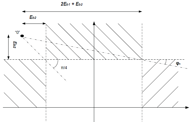
Figure 4: Decision boundaries and decoding for the PNC-mapped combined symbol 0

IV-B SER of the PNC-mapped Combined Symbol “1”

To understand the decoding process for the symbol “1”, we use the signal constellation geometry in Fig. 3. As shown in Fig. 5, the channel-equalized symbol $X^{ELCE}$ is considered an error in this case when it is located in the shaded regions. The expression of $P_{e/1}^{Symbol}$ can be derived, using Eq. (18), as follows

$$P_{e/1}^{Symbol} =\frac{1}{\pi}\int_{0}^{\pi/2}{}_{2}F_{1}\left(1,\,2;\,\frac{3}{2};\,\frac{\overline{\gamma}}{4}\frac{\left[E_{b_{2}}\right]^{2}}{2\sigma^{2}sin^{2}\theta}\right)\,d\theta$$

$$+\frac{1}{\pi}\int_{0}^{\pi/2}{}_{2}F_{1}\left(1,\,2;\,\frac{3}{2};\,\frac{\overline{\gamma}}{4}\frac{\left[2E_{b_{1}}-E_{b_{2}}\right]^{2}}{2\sigma^{2}sin^{2}\theta}\right)\,d\theta$$

$$+\frac{1}{\pi}\int_{0}^{\pi/2}{}_{2}F_{1}\left(1,\,2;\,\frac{3}{2};\,\frac{\overline{\gamma}}{4}\frac{\left[E_{b_{2}}\right]^{2}}{2\sigma^{2}sin^{2}\theta}\right)\,d\theta$$

$$-\frac{1}{\pi}\int_{0}^{\pi/4}{}_{2}F_{1}\left(1,\,2;\,\frac{3}{2};\,\frac{\overline{\gamma}}{4}\frac{\left[E_{b_{2}}\right]^{2}}{2\sigma^{2}sin^{2}\theta}\right)\,d\theta$$

$$-\frac{1}{\pi}\int_{0}^{\pi/4}{}_{2}F_{1}\left(1,\,2;\,\frac{3}{2};\,\frac{\overline{\gamma}}{4}\frac{\left[E_{b_{2}}\right]^{2}}{2\sigma^{2}sin^{2}\theta}\right)\,d\theta$$

$$-\frac{1}{\pi}\int_{0}^{\pi/2-\varphi_{1}}{}_{2}F_{1}\left(1,\,2;\,\frac{3}{2};\,\frac{\overline{\gamma}}{4}\frac{\left[2E_{b_{1}}-E_{b_{2}}\right]^{2}}{2\sigma^{2}sin^{2}\theta}\right)\,d\theta$$

$$-\frac{1}{\pi}\int_{0}^{\varphi_{1}}{}_{2}F_{1}\left(1,\,2;\,\frac{3}{2};\,\frac{\overline{\gamma}}{4}\frac{\left[E_{b_{2}}\right]^{2}}{2\sigma^{2}sin^{2}\theta}\right)\,d\theta$$ (25)

where $\varphi_{1}=tan^{-1}\left\{\frac{E_{b_{2}}}{2E_{b_{1}}-E_{b_{2}}}\right\}$

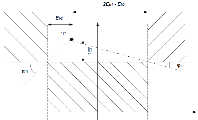
Figure 5: Decision boundaries and decoding for the PNC-mapped combined symbol 1

V Numerical Results

In this section, we present our numerical results for our proposed three-time-slot scheme in Fig. 2 and the end-to-end BER performance analysis for the received constellation shown in Fig. 3. Assume zero-mean white Gaussian noise and consider slow Rayleigh fading channels with flat amplitudes, we consider $E_{b_{1}}=4$, $E_{b_{2}}=2$, $E_{R}=1$, and $\overline{\gamma}=20dB$.

Fig. 6 depicts the end-to-end BER performance comparison between the proposed three-time-slot scheme and the resolvable BPSK and QPSK. Fig. 6 demonstrates that the proposed scheme achieves the same end-to-end BER performance of the resolvable BPSK and QPSK with higher spectral efficiency.

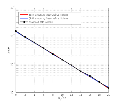
Figure 6: BER performance comparison between the proposed three-time-slot transmission scheme and resolvable BPSK and QPSK

In Fig. 7, we compare between the the simulation results of end-to-end BER for the proposed three-time-slot scheme and the others from the analytical expression for BER numerically calculated from Eq. (23). Fig. 7 demonstrates that the analytical expression for the end-to-end BER is consistent with the simulation results.

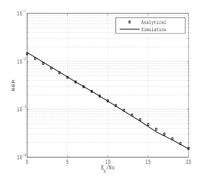
Figure 7: Comparison between analytical and simulation results for the proposed three-time-slot transmission scheme

VI Conclusion

In this paper, we proposed a novel three-time-slot transmission scheme combined with an efficient ELCE technique. Using such three-time-slot transmission scheme, we achieved about $33\%$ increase in the spectral efficiency over the conventional two-time-slot scheme with the same end-to-end BER performance as shown in our numerical results. In addition, we provided an exact expression for the end-to-end BER for the proposed three-time-slot scheme in case of BPSK transmission. Numerical results demonstrate that the provided exact analytical expression of the end-to-end BER of the proposed three-time-slot scheme is almost consistent with the BER simulation results.

References

• [1] H.ย Yang, W.ย Meng, B.ย Li, and G.ย Wang, โ€œPhysical layer implementation of network coding in two-way relay networks,โ€ in ICC โ€™12, 2012.
• [2] Y.ย Sagduyu and A.ย Ephremides, โ€œCrosslayer design for distributed MAC and network coding in wireless ad hoc networks,โ€ in ISIT โ€™05, 2005.
• [3] J.-S. Park, D.ย Lun, F.ย Soldo, M.ย Gerla, and M.ย Medard, โ€œPerformance of Network Coding in Ad Hoc Networks,โ€ in MILCOM โ€™06, 2006.
• [4] S.ย Zhang, S.ย C. Liew, and P.ย P. Lam, โ€œHot Topic- Physical-layer Network Coding,โ€ in ACM MobiCom 2006, Sept. 2006.
• [5] S.-Y.ย R. Li, R.ย Yeung, and N.ย Cai, โ€œLinear Network Coding ,โ€ IEEE Transactions on Information Theory, vol.ย 49, pp. 1204โ€“1216, Feb. 2003.
• [6] R.ย Ahlswede, N.ย Cai, S.-Y.ย R. Li, and R.ย W. Yeung, โ€œNetwork Information Flow,โ€ IEEE Transactions on Information Theory, vol.ย 46, no.ย 4, pp. 1204โ€“1216, Jul July 2000.
• [7] K.ย Lu, S.ย Fu, Y.ย Qian, and H.-H. Chen, โ€œSER Performance Analysis for Physical Layer Network Coding over AWGN Channels,โ€ in GLOBECOM 2009, Honolulu, Nov. 2009.
• [8] J.ย W. Craig, โ€œA New, Simple and Exact Result for Calculating the Probability of Error for Two-Dimensional Signal Constellations,โ€ in Milcom 1991, Nov. 1991.
• [9] B.ย Jiang, F.ย Gao, X.ย Gao, and A.ย Nallanathan, โ€œChannel estimation and training design for two-way relay networks with power allocation,โ€ IEEE Transactions on Wireless Communications, vol.ย 9, pp. 2022โ€“2032, June 2010.
• [10] F.ย Gao, R.ย Zhang, and Y.ย C. Liang, โ€œOptimal Channel Estimation and Training Design for Two-way Relay Networks,โ€ IEEE Transactions on Communications, vol.ย 57, Oct. 2009.
• [11] G.ย Wang, F.ย Gao, and C.ย Tellambura, โ€œJoint Frequency Offset and Channel Estimation Methods for Two-way Relay Networks,โ€ in Globecom 2009, Nov. 2009.
• [12] M.ย K. Simon and M.-S. Alouini, Digital Communication Over Fading Channels.ย ย ย John Wiley, 2005.
• [13] M.ย O. Hasna and M.-S. Alouini, โ€œEnd-to-End Performance of Transmission Systems With Relays Over Rayleigh-Fading Channels,โ€ IEEE Transactions on Wireless Communications, vol.ย 2, 2003.