Large scale clustering measurements with photometric redshifts: comparing the dark matter halos of X-ray AGN, star-forming and passive galaxies at $z\approx 1$

Abstract

We combine multiwavelength data in the AEGIS-XD and C-COSMOS surveys to measure the typical dark matter halo mass of X-ray selected AGN [$L_{X}(\rm 2-10\,keV)>10^{42}\,erg\,s^{-1}$] in comparison with far-infrared selected star-forming galaxies detected in the Herschel/PEP survey (PACS Evolutionary Probe; $L_{IR}>10^{11}\,L_{\odot}$) and quiescent systems at $z\approx 1$. We develop a novel method to measure the clustering of extragalactic populations that uses photometric redshift Probability Distribution Functions in addition to any spectroscopy. This is advantageous in that all sources in the sample are used in the clustering analysis, not just the subset with secure spectroscopy. The method works best for large samples. The loss of accuracy because of the lack of spectroscopy is balanced by increasing the number of sources used to measure the clustering. We find that X-ray AGN, far-infrared selected star-forming galaxies and passive systems in the redshift interval $0.6<z<1.4$ are found in halos of similar mass, $\log M_{DMH}/(M_{\odot}\,h^{-1})\approx 13.0$. We argue that this is because the galaxies in all three samples (AGN, star-forming, passive) have similar stellar mass distributions, approximated by the $J$-band luminosity. Therefore all galaxies that can potentially host X-ray AGN, because they have stellar masses in the appropriate range, live in dark matter haloes of $\log M_{DMH}/(M_{\odot}\,h^{-1})\approx 13.0$ independent of their star-formation rates. This suggests that the stellar mass of X-ray AGN hosts is driving the observed clustering properties of this population. We also speculate that trends between AGN properties (e.g. luminosity, level of obscuration) and large scale environment may be related to differences in the stellar mass of the host galaxies.

1 Introduction

In recent years progress has been made in our understanding of the physical conditions under which supermassive black holes (SMBHs) at the centres of galaxies grow their masses. Large extragalactic survey programs combining information from different parts of the electromagnetic spectrum made possible the study of the properties of the galaxies that host Active Galactic Nuclei (AGN), which signpost accretion events onto SMBHs. As a result constraints have been placed on e.g. the morphology (Georgakakis et al., 2009; Cisternas et al., 2011; Kocevski et al., 2012), stellar mass distribution (Bundy et al., 2008; Georgakakis et al., 2011; Aird et al., 2012) and position on the cosmic web (e.g. Coil et al., 2009; Mountrichas & Georgakakis, 2012; Mountrichas et al., 2013; Krumpe et al., 2012; Allevato et al., 2012; Krumpe et al., 2013; Komiya et al., 2013) of the hosts of AGN over a range of redshifts and accretion luminosities. These diagnostics of the physical conditions on large scales (kpc and Mpc) have also been related to the accretion properties of the SMBH, e.g. specific accretion rate or Eddington ratio (e.g. Schawinski et al., 2010; Aird et al., 2012, 2013), to better understand what triggers AGN and how they affect their immediate environment.

The general picture emerging from these studies is that at least in a statistical sense, star-formation episodes are related to the growth of SMBHs. The star-formation rate of galaxies for example, when integrated over cosmological volumes, evolves with redshift in the same manner as the AGN accretion density (Zheng et al., 2009; Aird et al., 2010). Similarly, the mean specific star-formation rate of galaxies also appears to follow the same evolution pattern as the AGN population (Georgakakis et al., 2011; Santini et al., 2012; Mullaney et al., 2012). Stacking the far-infrared fluxes at the positions of AGN shows that these systems at any given redshift lie, on the average, on or perhaps even above the main star-formation sequence of galaxies (Santini et al., 2012; Mullaney et al., 2012; Rovilos et al., 2012; Rosario et al., 2013). At the same time however, it has been become clear that in individual AGN there is no one-to-one correspondence between the level of star-formation in the host galaxy and the accretion luminosity (Shao et al., 2010; Mullaney et al., 2012; Rosario et al., 2012). There is rather substantial scatter in the star-formation/accretion-luminosity diagram of AGN. This can be interpreted as a manifestation of the long term variability of AGN and ultimately the different timescales of star-formation and black hole growth (Hickox et al., 2013).

The large scatter in the star-formation properties of individual AGN could also be understood in the context of different SMBH fueling modes that operate in galaxies with distinct cold gas reservoirs and hence, star-formation histories. Evidence for a dichotomy in the accretion rate distribution of AGN based on the star-formation history of their hosts is found at low redshifts, $z\la 0.1$ (Kauffmann & Heckman, 2009). AGN associated with the most actively star-forming galaxies have high Eddington ratios that follow a log-normal distribution. In contrast, active SMBHs in quiescent galaxies are characterised by low Eddington ratios that are distributed as a power-law. Evidence also exists that these trends between the level of star-formation of galaxies and the Eddington ratio of AGN persist to higher redshift, $z\approx 1$ (Georgakakis et al. 2014 in prep.; but see Aird et al. 2012). The observed large-scale clustering properties of X-ray AGN are also consistent with models (Fanidakis et al., 2012) that postulate two channels for growing SMBHs, each one of which takes place in galaxies with very different star-formation histories (Fanidakis et al., 2013).

In this paper we explore the relation between AGN activity and star-formation by measuring the typical dark matter halo mass of X-ray AGN in comparison with star-forming galaxies detected in the far-infrared by the Herschel space telescope. If the bulk of the black hole growth is related to star-formation events then one might expect similar large scale environments for X-ray AGN and Herschel sources. Moreover, if there is an AGN sub-population associated with passive and strongly clustered hosts we might be able to identify its signatures in large scale clustering measurements.

We address these questions by developing a novel clustering estimation method that uses photometric redshifts, in the form of probability distribution functions, in addition to any available spectroscopy, to estimate the projected correlation function of any extragalactic population. This is motivated by the significant improvement in recent years in the quality and quantity of photometric redshift estimates for both AGN and galaxies. The method is geared toward large sample sizes to minimise the impact of photometric redshift uncertainties onto the clustering signal. It is therefore well suited for measurements of the clustering of AGN in e.g. the eROSITA All Sky Survey (Merloni et al., 2012). One of the advantages of the new clustering estimator is that one can use in the analysis all sources (e.g. X-ray AGN, Herschel galaxies) with optical counterparts in a sample, not just the optically brighter ones for which spectroscopy is available. This method extends clustering measurement techniques based on photometric redshift PDFs developed and/or applied to data by Myers et al. (2009), Hickox et al. (2011, 2012) and Mountrichas et al. (2013). These methods are geared toward the determination of the projected cross-correlation function between two extragalactic populations and require spectroscopic redshifts for at least one of the two samples. In contrast, the method presented here allows clustering measurements (auto-correlation or cross-correlation) via the projected correlation function, even at the limiting case of no spectroscopic information for any of the galaxy populations involved. Throughout this paper we adopt $H_{0}=100$ km s^-1 Mpc^-1, $\Omega_{m}=0.3$ and $\Omega_{\Lambda}=0.7$ and $\sigma_{8}=0.8$. Rest frame quantities (e.g. luminosities, dark matter halo masses) are parametrised by $h=H_{0}/100$, unless otherwise stated.

Figure 1: Normalised redshift distribution of galaxies in the combined C-COSMOS and CFHTLS-D3 fields after applying the $B-R$ and $R-I$ colour cuts defined by Newman et al. (2012) to pre-select galaxies at $z>0.6$. The magnitude limit of the two samples is set to $R=24.5$ mag. The redshift distribution is estimated by summing the photometric redshift PDFs of individual galaxies. The corresponding cumulative redshift distribution is shown in the inset plot. It shows that about 80% of the sample is in the redshift range 0.6-1.4.

Figure 2: $U-V$ vs $V-J$ diagram of galaxies (black contours) in the AEGIS-XD and C-COSMOS fields with $R<24.5$ and either spectroscopic or photometric redshift estimates. For sources with photometric redshifts we use the full PDFs to determine the corresponding $U-V$, $V-J$ probability distribution functions. The different contour levels correspond to 1000, 700, 400, 200 and 100 galaxies within bins of size 0.1 mag. The dashed lines correspond to $U-V=0.88\,(V-J)+0.69$, $U-V>1.3$, $V-J<1.6$ (Williams et al. 2009). Galaxies are distributed into two distinct populations, i.e. quiescent and star-forming. The wedge, as defined above, marks the transition region between these two galaxy populations. The arrow shows the reddening vector with $A_{V}=1$ for the Calzetti et al. (2000) law. This is parallel to the quiescent galaxy selection wedge. Dusty star-forming galaxies are therefore separated from quiescent systems.

2 The data

Two extragalactic survey fields are used to determine the clustering of X-ray AGN and infrared selected galaxies at $z\approx 1$. The All Wavelength Extended Groth strip International Survey (AEGIS, Davis et al., 2007) and the Cosmological evolution Survey (COSMOS, Scoville et al., 2007). The choice of fields is motivated by the availability of (i) deep Chandra and Herschel data, (ii) extensive follow-up spectroscopic programs targeting specifically X-ray sources and (ii) deep multiwavelength imaging (UV, optical, infrared) for the determination of photometric redshift Probability Distribution Functions (PDFs) for galaxies and AGN. In the subsequent analysis we focus on the part of the AEGIS field which has been surveyed by Chandra for a total of 800 ks (AEGIS-XD, Nandra et al. in prep). In the COSMOS field we use the region covered by the Chandra observations performed between November 2006 and June 2007 (C-COSMOS, Elvis et al., 2009). Combining clustering measurements from two extragalactic survey fields gives a better handle on the impact of cosmic variance on the results.

2.1 The galaxy samples

The AEGIS-XD field lies within the D3 region of the deep synoptic Canada-France-Hawaii Telescope Legacy Survey (CFHTLS). The optical photometry ($ugriz$ bands) of the T0004 data release is used, which includes photometric redshift measurement and their corresponding PDFs with an estimated dispersion at the limit $i<24$ mag of $\sigma_{\Delta z/(1+z)}\approx 0.03$ (Coupon et al., 2009). Regions of unreliable photometry (CFHTLS catalogue parameter flag_terapix$>1$) because e.g. of contamination by bright stars, are masked out. In the analysis we only use CFHTLS optical sources classified as galaxies (CFHTLS parameters object and flag_terapix equal to zero), with reliable photometric redshift estimates (CFHTLS parameter zp_reliable$\neq-99$).

For the C-COSMOS field we use the version 1.8 of the photometric redshift catalogue of Ilbert et al. (2009), which includes PDFs for the photometric redshifts and is based on an improved version of the photometry originally presented by Capak et al. (2007). The accuracy of the photometric redshifts to $i=24$ mag is $\sigma_{\Delta z/(1+z)}\approx 0.01$ (Ilbert et al., 2009). Spatial masks defined in the $B$, $V$, $i$ and $z$ photometric bands have been used to identify and exclude from the analysis sources which lie in regions with unreliable photometry. Optical sources with Spectral Energy Distributions (SEDs) that are best-fit by stellar templates (Ilbert et al., 2009) are also excluded.

In the clustering analysis presented in the later sections the photometric galaxy samples in the AEGIS-XD and C-COSMOS fields are limited to redshifts $z\ga 0.6$. The $B-R$ and $R-I$ photometric criteria for redshift pre-selection defined by Newman et al. (2012, i.e. $B-R<2.35\,(R-I)-0.45$, $R-I>1.15$, $B-R<0.5$) are adopted to exclude galaxies below $z\approx 0.6$. The resulting redshift distribution is plotted in Fig. 1. Nearly 80% of the galaxy sample lies in the redshift interval $0.6<z<1.4$. For the application of the above colour cuts the AEGIS-XD/CFHTLS and C-COSMOS filtersets are transformed to the $BRI$ photometric bands used by Newman et al. (2012) following the methods described in Mountrichas et al. (2013). Unless otherwise stated the galaxy samples used in the following sections are also limited to the magnitude range $18<R<24.5$ mag to ensure reliable photometric redshift determinations and PDFs (Ilbert et al., 2009; Coupon et al., 2009). In the clustering measurements described below only the part of the galaxies’ photometric redshift PDF in the range $0.6<z<1.4$ is used.

2.2 Far-infrared galaxies

Herschel far-infrared (far-IR) data are from the PACS Evolutionary Probe (PEP; Lutz et al., 2011) programme, which has surveyed, among others, the AEGIS-XD and C-COSMOS fields at 100 and $\rm 160\mu m$. We use the PEP source catalogues constructed by fitting the PACS PSF at the positions of sources detected on archival Spizter MIPS $24\mu m$ data following the method of Magnelli et al. (2009). The $3\sigma$ depths at $\rm 100/160\mu m$ in the AEGIS-XD and C-COSMOS fields are approximately 4/8 and 5/11 mJy, respectively. The PEP source positions were matched to the closest optical counterpart using a search radius of 1.5 arcsec. The false identification rate at the limit $i=24$ mag is 3.5%. Total IR luminosities , $L_{IR}$, in the wavelength range $8-1000\,\mu m$ are determined from the PEP $\rm 100/160\mu m$ flux densities assuming the $L_{IR}=10^{11}\,L_{\odot}$ template of Chary & Elbaz (2001).

The prime interest of this paper is the clustering properties of infrared galaxies at $z\approx 1$. We therefore select PEP sources in the redshift interval $0.6<z<1.4$. For sources with photometric redshift measurements we only use the part of the PDF that lies within that redshift range. We do not apply any IR luminosity cut to the sample. At the redshift interval $0.6<z<1.4$, the PEP survey depths of the AEGIS-XD and C-COSMOS fields correspond to $L_{IR}\ga 10^{11}\,L_{\odot}$. For the typical stellar mass of the PEP far-IR selected galaxies ($\rm\approx 10^{11}\,M_{\odot}$; see later sections) the luminosity limit above corresponds to galaxies on or just above the main sequence of star-formation (Santini et al., 2009) at $z\approx 1$. Table 1 shows for each field the number of PEP far-IR selected galaxies used for clustering measurements.

2.3 The X-ray AGN samples

We use X-ray data from the Chandra 800 ks survey of the AEGIS-XD field (Nandra et al. in prep) and the 2006-2007 Chandra survey of the C-COSMOS field (Elvis et al., 2009). The Chandra observations of the AEGIS-XD and C-COSMOS were analysed in a homogeneous way by applying the reduction and source detection methodology described by Laird et al. (2009). The optical identification of the X-ray sources was based on the Likelihood Ratio method (Sutherland & Saunders, 1992). In the case of the AEGIS-XD we used the IRAC-$\rm 3.6\mu m$ selected multi-waveband photometric catalogue provided by the Rainbow Cosmological Surveys Database (Pérez-González et al., 2008; Barro et al., 2011a, b). The identification of C-COSMOS X-ray sources used the Ilbert et al. (2009) multiwavelength photometric catalogue (Aird et al. in prep).

Extensive spectroscopic campaigns have been carried out in the fields of choice. Spectroscopic redshift measurements of X-ray sources in the AEGIS-XD field are primarily from the DEEP2 (Newman et al., 2012) and DEEP3 galaxy redshift surveys (Cooper et al., 2011, 2012) as well as observations carried out at the MMT using the Hectospec fibre spectrograph (Coil et al., 2009). Redshifts in C-COSMOS are from the public releases of the VIMOS/zCOSMOS bright project (Lilly et al., 2009) and the Magellan/IMACS observation campaigns (Trump et al., 2009), as well as the compilation of redshifts for X-ray sources presented by Brusa et al. (2010).

For X-ray sources without spectroscopic identifications care is needed when determining photometric redshifts because of the contribution of AGN light to the observed SED. Salvato et al. (2009, 2011) showed that for X-ray AGN it is possible to achieve photometric redshift accuracies comparable to galaxy samples by (i) adopting priors for the templates used for each source, (ii) icluding hybrid AGN/galaxy templates and (iii) increasing the number of photometric bands used to sample the observed SED. For X-ray AGN we therefore use the photometric redshift PDFs estimated using the methods of Salvato et al. (2009, 2011). These are presented in Salvato et al. (2011) for C-COSMOS and Nandra et al. (in prep) for the AEGIS-XD. The estimated rms scatter of the X-ray AGN photometric redshifts is $\sigma_{\Delta z/(1+z)}=0.016$ and 0.04 for the C-COSMOS and AEGIS-XD samples, respectively. The corresponding outlier fraction, defined as $\Delta z/(1+z)>0.15$, is about 6% in both fields.

A by-product of the photometric redshift determination is the characterisation of the Spectral Energy Distribution (SED) of X-ray AGN, e.g. host galaxy type, level of optical extinction, level of the AGN component relative to the underlying host galaxy. The latter information is used in later sections to identify sources for which the AGN radiation likely contaminates the host galaxy light. Far-IR counterparts to X-ray AGN are identified by matching the PEP and optical source catalogues in AEGIS-XD and C-COSMOS within a search radius of 1.5 arcsec.

The intrinsic column density, $N_{H}$, of individual X-ray AGN is determined from the hardness ratios between the soft (0.5-2 keV) and the hard (2-7 keV) X-ray bands assuming an intrinsic power-law X-ray spectrum with index $\Gamma=1.9$ (e.g. Nandra & Pounds, 1994). The derived column densities are then used to convert the count-rates in the 0.5-7 keV band to rest-frame 2-10 keV luminosity, $L_{X}(\rm 2-10\,keV)$. For sources with photometric redshift PDF, the X-ray luminosity is also a probability distribution function. In the clustering analysis we use X-ray sources with $L_{X}(\rm 2-10\,keV)>10^{42}\,erg\,s^{-1}$ and redshifts $0.6<z<1.4$. For X-ray sources with photometric redshift estimates we retain in the analysis only the part of their PDF that corresponds to the limits above. X-ray sources in regions that have been masked out because of poor optical photometry (e.g. bright stars) are excluded from the analysis. Table 1 presents for each field the number of X-ray AGN and the number of X-ray AGN with far-IR counterparts in the PEP survey.

2.4 Passive galaxies

In the following sections the clustering of X-ray AGN and IR-selected star-forming galaxies will be compared to that of quiescent galaxies. The latter are selected using the rest-frame $U-V$ vs $V-J$ (UVJ) colour-colour diagram (Williams et al., 2009; Patel et al., 2012). This combination of colours is least sensitive to dust extinction and is shown to be effective in separating early-type, low-specific star-formation rate galaxies from actively star-forming, including dust-reddened systems (Williams et al. 2009).

Figure 2 plots the UVJ diagram of galaxies with $18<R<24.5$ mag and $0.6<z<1.4$ in the AEGIS-XD and C-COSMOS fields. The rest-frame $U-V$ and $V-J$ colours are estimated by the kcorrect version 4.2 routines. For AEGIS-XD the CFHTLS-D3 $ugriz$ and Palomar WIRC $JK$ (Bundy et al., 2006) photometry is provided to kcorrect. In C-COSMOS fluxes in the CFHT $u^{\star}$, SUBARU $Vg^{+}r^{+}i^{+}z^{+}$ (Capak et al., 2007), UKIRT WFCAM $J$ (McCracken et al., 2010) and CFHT WIRCAM $Ks$ (Capak et al., 2007) filters are used. Rest-frame $U$, $V$ and $J$ luminosities are determined from the observed photometry in the $r/r^{+}$, $z/z^{+}$ and $K/Ks$ bands of AEGIS-XD/C-COSMOS, respectively. This choise of bands is to minimise k-corrections. For sources with photometric redshift estimates the $U-V$, $V-J$ rest-frame colours are estimated separately for each bin of the photometric redshift probability distribution function. For each of these sources a given ($U-V$, $V-J$) pair, which corresponds to a photometric redshift bin $z\pm\delta z$ of the PDF, is assinged a weight which is the probability that the source lies in the interval $z\pm\delta z$ (i.e. the corresponding value of the photometric redshift PDF). When constructing the contours of Figure 2, sources with photometric redshifts contribute with different weights to different ($U-V$, $V-J$) bins.

In Figure 2 quiescent systems are separated from star-forming (including dusty) galaxies by the selection wedge defined by the relations $U-V>1.3$, $V-J<1.6$ and $U-V>0.88\,(V-J)+0.69$ (Williams et al., 2009). The specific star-formation rate of galaxies is found to change rapidly across the wedge, at least for redshifts $z\la 1.5$ (Williams et al., 2009). For the clustering analysis we use sources in the passive region of the UVJ diagram, i.e. $U-V>1.3$, $V-J<1.6$ and $U-V>0.88\,(V-J)+0.69$. For galaxies with photometric redshift PDFs we use only the part of the PDF with corresponding $U-V$, $V-J$ within the quiescent wedge of the UVJ diagram. Table 1 presents for each field the number of $UVJ$ passive galaxies used in the analysis. In addition to the optical magnitude ($18<R<24.5$ mag) and redshift ($0.6<z<1.4$) cuts these samples are also selected to include only galaxies that are bright in absolute $J$-band magnitude, $M_{J}<-21.5$ mag (see next section).

2.5 $J$-band luminosities

For the interpretation and comparison of the clustering properties of X-ray AGN, star-forming and passive galaxies we also explore the relative stellar mass distribution of their host galaxies. We use the $J$-band absolute magnitude, $M_{J}$, as proxy of stellar mass. The advantage of using luminosities in a near-IR band to approximate stellar mass is because the corresponding mass–to–light ratios are less sensitive to the star-formation history of the galaxy (e.g. Bell et al., 2003).

The kcorrect is used to estimate the rest-frame absolute magnitudes (AB system) of extragalactic sources in the 2MASS-$J$ filter. The input photometry to kcorrect is the same as in section 2.4.

To minimise k-corrections, which unavoidably depend on the adopted set of model spectral energy distributions, the rest-frame magnitude of a source in the $J$ filter is estimated from the observed photometry in $K$-band. At $z\approx 1$ the $K$-band effective wavelength (observer frame) is close to that of the $J$-band filter at the rest-frame of the source. When $K$-band is not available we use the observed $J$ band magnitude to determine $M_{J}$. For sources with photometric redshifts the $M_{J}$ is a probability distribution function. We also exclude X-ray sources for which the SED fitting process described in section 2.3 suggests a significant AGN component that could contaminate the host galaxy emission. For those sources $M_{J}$ may not be a proxy of stellar mass.

Table 1: Details on the samples used for clustering measurements. We list for each field separately (C-COSMOS, AEGIS-XD) and the combined dataset (“Total”) the number of X-ray AGN, far-IR selected galaxies in the PEP survey, UVJ passive galaxies and X-ray AGN with far-IR counterparts. The numbers are sources with either spectroscopic redshifts in the range $0.6<z<1.4$ or photometric redshifts with PDF that at least partially overlaps with the redshift interval above. The number of sources in each sample with spectroscopic redshifts are presented in the parenthesis. The last row of the table lists the total number of optically selected galaxies used to determine their auto-correlation function. They are select to have $R<24.5$ and to satisfy the $B-R$ vs $R-I$ colour cuts defined by Newman et al. (2012) to photometrically pre-select galaxies at $z>0.6$.

Sample	C-COSMOS	AEGIS-XD/CFHTLS-D3	Total
X-ray AGN	498 (282)	771 (148)	1269 (430)
PEP far-IR galaxies	578 (225)	454 (351)	1032 (576)
X-ray AGN with far-IR IDs	78 (50)	103 (34)	181 (84)
UVJ passive	4087 (375)	817 (421)	4883 (796)
galaxies	32,699	35,991	68,690

Table 2: Power-law best-fit parameters $r_{0}$, $\gamma$ estimated at scales 1–10 Mpc for the cross-correlation function between different samples (X-ray AGN, far-IR sources, X-ray AGN with/without far-IR counterparts, passive systems) and optical galaxies and the auto-correlation function of optical galaxies. The inferred biases and mean dark matter halo masses are also listed. The columns are: (1): sample for which the clustering properties are estimated. The clustering statistics of the galaxy auto-correlation function are listed in the last row; (2): median redshift of each sample; (3): best-fit power-law clustering scale $r_{o}$ of the cross-correlation function with optical galaxies or the auto-correlation function for the galaxy sample (last row); (4): best-fit power-law index $\gamma$ of the cross-correlation function with optical galaxies or the auto-correlation function for the galaxy sample (last row); (5): reduced $\chi^{2}$ and degrees of freedom for the power-law fits to the correlation function; (6): cross-correlation function bias parameter, $b_{CCF}$; (7): auto-correlation function bias parameter, $b_{ACF}$. For galaxies this is determined directly by measuring their auto-correlation function (last row). For X-ray AGN, PEP far-IR selected galaxies, UVJ passive galaxies, and PEP/X-ray AGN, $b_{ACF}$ is inferred from $b_{CCF}$ (column 6) after factoring out the galaxy auto-correlation function bias listed in the last row of the table; (8): corresponding mean dark matter halo mass.

Sample	median	$r_{0}$	$\gamma$	$\chi^{2}$/dof	$b_{CCF}$		$b_{ACF}$	$\rm\log M_{DMH}$
	redshift	($h^{-1}$ Mpc)						($h^{-1}$ M⊙)
(1)	(2)	(3)	(4)	(5)	(6)		(7)	(8)
	Cross-correlation function with galaxies
X-ray AGN	0.95	$4.8^{+0.7}_{-0.6}$	$1.9^{+0.1}_{-0.2}$	0.2/8	$1.8^{+0.2}_{-0.2}$		$2.0^{+0.5}_{-0.4}$	$13.0^{+0.3}_{-0.4}$
PEP far-IR galaxies	0.90	$4.9^{+1.0}_{-0.8}$	$1.8^{+0.1}_{-0.1}$	0.3/8	$1.8^{+0.3}_{-0.2}$		$2.0^{+0.6}_{-0.5}$	$13.0^{+0.4}_{-0.5}$
X-ray AGN with far-IR IDs	0.95	$4.9^{+1.5}_{-1.3}$	$1.9^{+0.2}_{-0.2}$	0.8/8	$1.8^{+0.5}_{-0.4}$		$2.1^{+1.1}_{-1.0}$	$13.0^{+0.6}_{-1.5}$
X-ray AGN w/out far-IR IDs	0.97	$5.3^{+1.1}_{-1.1}$	$1.9^{+0.2}_{-0.1}$	1.5/8	$1.8^{+0.2}_{-0.2}$		$2.1^{+0.5}_{-0.5}$	$13.1^{+0.4}_{-0.4}$
UVJ passive	0.84	$5.1^{+0.6}_{-0.9}$	$1.6^{+0.2}_{-0.2}$		$1.7^{+0.1}_{-0.2}$	0.3/8	$1.8^{+0.3}_{-0.5}$	$12.9^{+0.3}_{-0.7}$
	Auto-correlation function of galaxies
galaxies	0.90	$4.6^{+0.6}_{-0.5}$	$1.8^{+0.2}_{-0.1}$	0.2/8	–		$1.6^{+0.1}_{-0.2}$	–

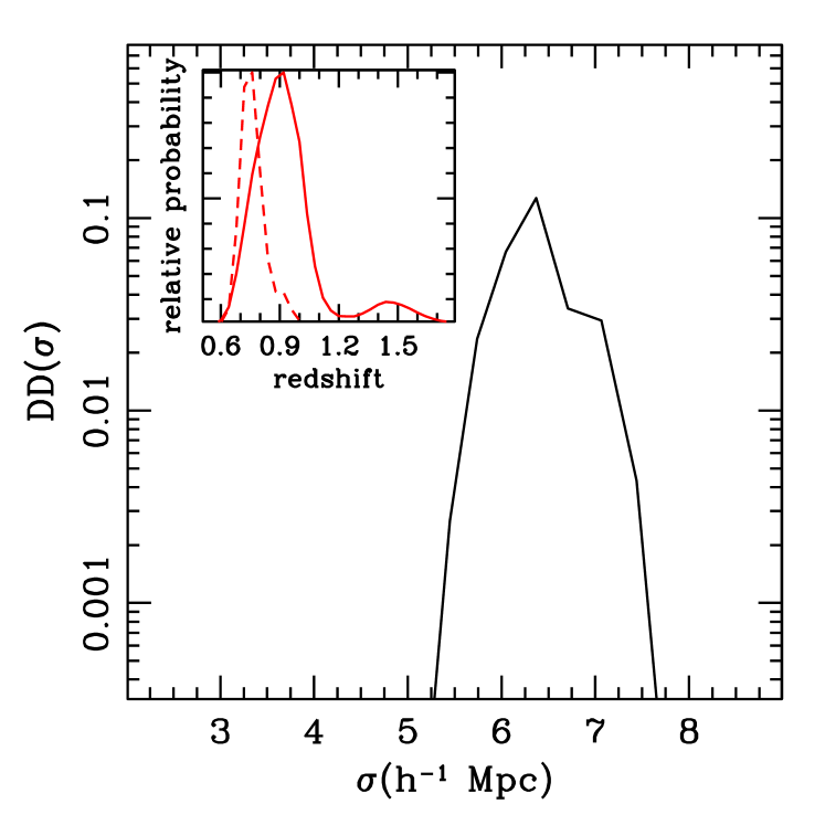
Figure 3: Demonstration of the DD determination in the case of the generalised clustering estimator using photometric redshift information. DD($\sigma$) is plotted as a function of scale for a randomly chosen galaxy-galaxy pair in the AEGIS-XD field. The inset plot shows the photometric redshift PDFs (red dotted and solid black curves) of the two galaxies. Intuitively, DD in the generalised clustering estimator method can be thought of as the product of the convolution of the two photometric redshift PDFs.

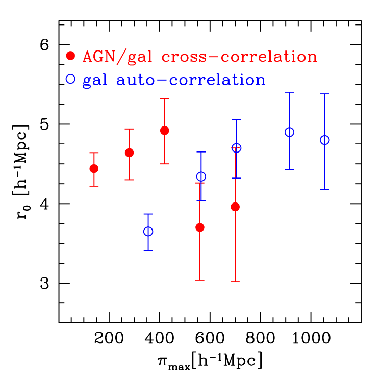
Figure 4: Correlation function length, $r_{0}$, as a function of $\pi_{max}$, the maximum scale of the integration in equation 5. The filled (red) circles are for the AGN/galaxy cross-correlation function. The open circles are for the galaxy auto-correlation function. The errors are jackknife.

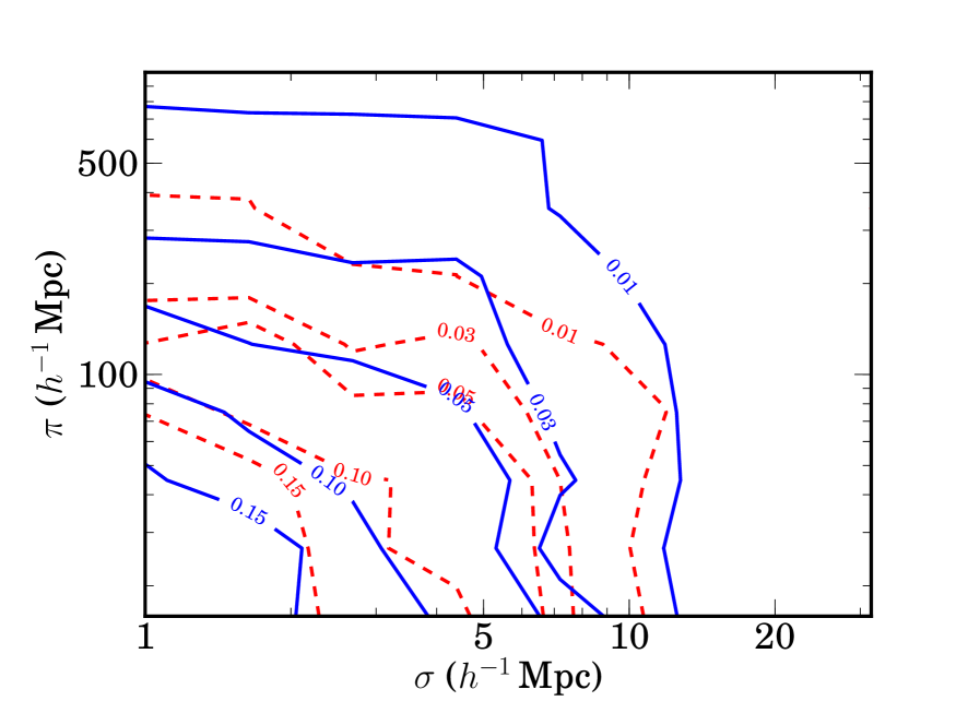
Figure 5: Redshift-space correlation function, $\xi(\sigma,\pi)$. The blue solid contours correspond to the galaxy auto-correlation function. The red dashed contours are the AGN/galaxy cross-correlation function. The numbers on the contours represent the value of $\xi(\sigma,\pi)$. The elongations along the $\pi$ direction (y-axis) are because of peculiar velocities and photometric redshift uncertainties. The contours show that the integration of the $\xi(\sigma,\pi)$ to $\pi_{max}=450$, 700 Mpc for the AGN/galaxy cross-correlation and the galaxy auto-correlation functions respectively, includes the bulk of the clustering signal.

3 Methodology: generalised clustering estimator for photometric redshift samples

Next we present the equations used to determine the clustering of any extragalactic population such as AGN or galaxies. Both the auto-correlation and the cross-correlation functions are special cases of the 2-point statistics of the AGN and galaxy populations. Therefore, they are both defined by the same basic equations. In this section the term correlation function refers to either the auto-correlation or the cross-correlation functions. When necessary we will differentiate between the two quantities. The real-space correlation function, $\xi(r)$, can be estimated by the relation (Davis & Peebles, 1983)

$$\xi(r)=\frac{DD(r)}{DR(r)}-1,$$ (1)

where DD(r) are the data-data pairs at separation $r$. DR(r) are the AGN-random pairs (cross-correlation) or galaxy-random pairs (galaxy auto-correlation function) at separation $r$. Both DD and DR in equation 1 are normalised appropriately. Random catalogues are produced by randomising the position of galaxies, taking into account the sample selection function, i.e. magnitude limit, field boundaries, masked regions. We choose to construct random catalogues for the galaxy (tracer) sample. This is because the spatial selection function of the X-ray AGN in particular, is complex and varies across the field of view of individual Chandra pointings. These variations might introduce systematics into the calculations unless they are quantified to a high degree of accuracy.

The distance $r$ can be decomposed into separations along the line of sight, $\pi$, and across the line of sight, $\sigma$. If $s_{1}$ and $s_{2}$ are the distances of two objects 1, 2, measured in redshift-space, and $\theta$ the angular separation between them, then $\sigma$ and $\pi$ are defined as

$$\pi=(s_{2}-s_{1}),$ along the line-of-sight$,$$ (2)

$$\sigma=\frac{(s_{2}+s_{1})}{2}\theta,$ across the line-of-sight$.$$ (3)

The correlation function in redshift-space is then estimated as

$$\xi(\sigma,\pi)=\frac{DD(\sigma,\pi)}{DR(\sigma,\pi)}-1.$$ (4)

In the classic approach of estimating the redshift-space correlation function, when accurate spectroscopic redshifts are available, each data-data pair with $\sigma$, $\pi$ separations is incremented by one, i.e. $DD(\sigma,\pi)=DD(\sigma,\pi)+1$. If the redshift determinations are uncertain, i.e. photometric redshifts, the above relation can be generalised to include those uncertainties, in the form of Probability Distribution Functions (PDF).

Suppose two data points, D1 and D2, which are associated with photometric redshift probability distribution functions $\rm PDF_{1}$ and $\rm PDF_{2}$, respectively. We assume that these PDFs are estimated at discrete photometric redshift data points with binsize $\delta z$. The value $f_{i}$ of a PDF at the bin $i$ is the probability that the source lies in the redshift range $z_{i}\pm\delta z/2$. Let us then assume a probability $f_{i,1}$, drawn from $\rm PDF_{1}$, that D1 lies in the redshift slice $z_{i}\pm\delta z/2$. The probability of D2 lying at separations $\sigma$, $\pi$ from D1 at $z_{i}$ can then be estimated from $\rm PDF_{2}$, e.g. $f_{i,2}$. The number of data-data pairs $DD(\sigma,\pi)$ is then incremented by the product $f_{i,1}\,f_{i,2}$, instead of unity, i.e. $DD(\sigma,\pi)=DD(\sigma,\pi)+f_{i,1}\,f_{i,2}$. In this picture DD(r) corresponds to a probability distribution function. Figure 3 shows an example of a single DD estimated for a particular galaxy-galaxy pair in the AEGIS-XD field. In this particular case the photometric redshift PDF has a binsize of $\delta z=0.01$. The $DR(\sigma,\pi)$ pairs are estimated following the same procedure. Each random point is assigned the photometric redshift PDF of one of the observed galaxies in the sample. The redshift distribution of random points is therefore similar to that of galaxies.

When the correlation function is measured in redshift-space, the clustering is affected at small scales by the peculiar velocity component of extragalactic sources along the line of sight and by dynamical infall of matter into higher density regions. In the case of the generalised clustering estimator photometric redshift uncertainties also have an impact on the radial component of $\xi(\sigma,\pi)$. These effects can be removed by integrating along the line of sight, $\pi$, to calculate the projected cross-correlation function

$$w_{p}(\sigma)=2\int_{0}^{\pi_{max}}\xi(\sigma,\pi)d\pi.$$ (5)

The maximum scale of the integration is a trade-off between underestimating the clustering amplitude, if $\pi_{max}$ is too small, and low signal-to-noise ratio, if $\pi_{max}$ is too large. The optimum $\pi_{max}$ value can be determined by either (i) measuring the projected correlation function for different $\pi_{max}$ and then adopting the value at which the amplitude of the cross-correlation function appears to level off or (ii) by inspecting how $\xi(\sigma,\pi)$ is distributed in $\sigma$, $\pi$ space and then determining the maximum $\pi$ value that includes most of the clustering signal.

The uncertainties of the correlation function at a given scale are estimated using the Jackknife methodology. The survey fields are divided into a total of $N_{JK}$ sections. The projected correlation function is re-estimated $N_{JK}$ times by excluding in each trial one of the sections. These measurements are then used to determine the covariance matrix, which quantifies the level of correlation between different different bins of $w_{p}(\sigma)$ (e.g. Krumpe et al., 2010). During this process it was found that the $w_{p}(\sigma)$ measured from individual Jackknife sub-samples do not follow the Normal distribution but are skewed by outliers. This effect is stronger in the case of the generalised clustering estimation method. We therefore choose to represent the uncertainties of the correlation function by the 16th and 84th percentiles of the distribution of $w_{p}(\sigma)$ measured from the $N_{JK}$ Jackknife sections.

The bias parameter for a given extragalactic population is estimated from the rms fluctuations of the density distribution over a sphere with a comoving radius of $8\,h^{-1}$ Mpc ($\sigma_{8}$) under the assumption that the correlation function follows a power-law (e.g. Mountrichas et al., 2013)

$$\sigma_{8}^{2}=J_{2}(\gamma)\left(\frac{r_{0}}{8h^{-1}Mpc}\right)^{\gamma},$$ (6)

where

$$J_{2}(\gamma)=\frac{72}{(3-\gamma)(4-\gamma)(6-\gamma)2^{\gamma}},$$ (7)

and $\gamma$, $r_{0}$ are the slope and amplitude of the power-law form of the correlation function. The bias is then calculated by the relation

$$b=\frac{\sigma_{8}}{\sigma_{8}(z)}.$$ (8)

where $\sigma_{8}(z)$ is the rms fluctuations of the dark matter density field within an $8\,h^{-1}$ Mpc sphere at redshift $z$. We account for the non-Gaussian errors of $w_{p}(\sigma)$ by determining separately for each Jackknife region the correlation function power-law parameters (slope, $\gamma$; amplitude, $r_{0}$) and the corresponding bias at scales 1-10 Mpc. The errors of each of those parameters are then represented by 16th and 84th percentiles of the distribution of the $N_{JK}$ measurements. The covariance matrix is used indirectly in the error estimation process to determine the best-fit power-law parameters for each Jackknife region.

We adopt the ellipsoidal collapse model of Sheth et al. (2001) and the analytical approximations of van den Bosch (2002) to infer the mean dark matter halo mass of an extragalactic population (AGN or galaxies) from the measured bias parameter. This calculation assumes that on large scales the bias depends only on halo mass.

Appendix A demonstrates the performance of the generalised clustering estimator that uses photometric redshifts PDFs. The results using this method are compared with clustering measurements based on spectroscopic samples only. It is shown that the method described in this section can recover the clustering signal of extragalactic populations even if no spectroscopic redshift information is available. Large photometric redshift samples are required however, at least 10 times larger than spectroscopic ones, to recover the clustering signal at the same level of accuracy.

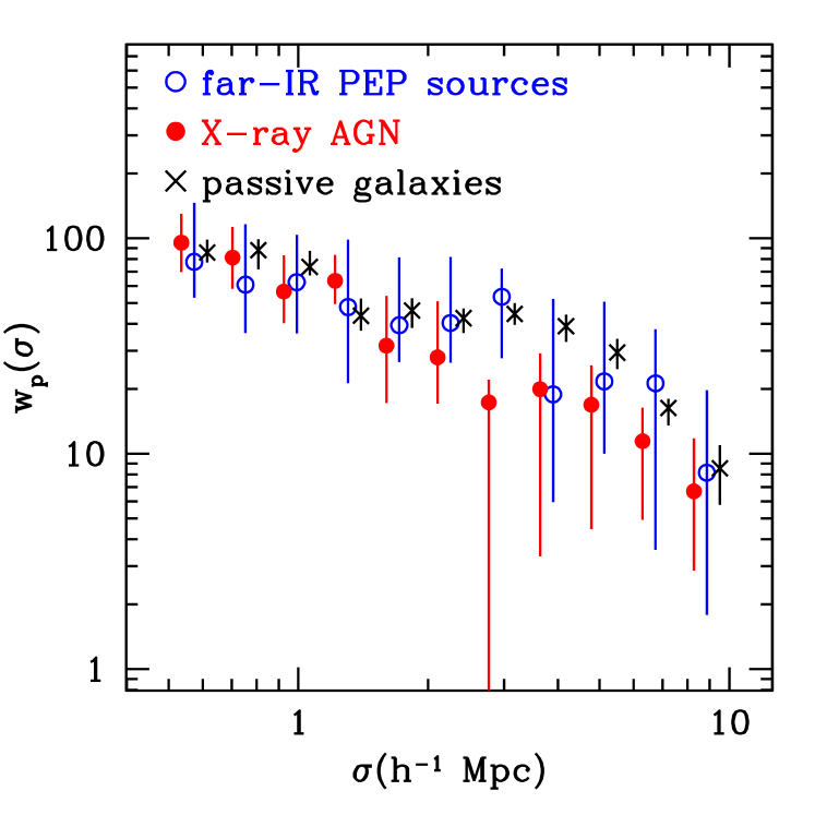
Figure 6: Left: Cross-correlation function with galaxies of (i) X-ray AGN (solid red circles), (ii) IR sources (empty blue circles) and (iii) $UVJ$ passive galaxies (black crosses), in the combined AEGIS-XD and C-COSMOS fields. The errorbars are Jackknife. The solid red symbols are offset in the horizontal direction by $\log=\pm 0.03$ for clarity. Right: Auto-correlation function of galaxies ($R<24.5$ mag) in the combined AEGIS-XD and C-COSMOS fields. The uncertainties of individual datapoints are estimated from $N_{JK}=16$ Jackknife sub-regions.

4 Results

In this section we estimate and compare the clustering properties of (i) X-ray AGN, (ii) far-IR selected sources detected in the PEP survey and (iii) passive galaxies selected by their $U-V$ and $V-J$ rest-frame colours (Williams et al., 2009; Patel et al., 2012). Differences/similarities of the large scale environment of those samples can provide clues on the association between AGN activity as traced by X-rays and the level of star-formation in galaxies. In this comparison one should also account for possible covariances between environment and galaxy properties other than instantaneous star-formation rate. One galaxy parameter that is known to correlate with large-scale environment is stellar mass (e.g. Mostek et al., 2012). Therefore in the interpretation of the clustering properties of the samples above we also include information on the stellar mass distribution of the underlying galaxies. Also, X-ray AGN and far-IR sources have similar redshift distributions that both peak at $z\approx 0.9$ (see Table LABEL:table:fits). Passive galaxies however, because of their red SEDs, have a distribution that peaks at somewhat lower redshift, $z=0.84$ (see Table LABEL:table:fits). In the following calculations and unless otherwise stated, we use both photomertric redshifts PDFs and spectroscopic redshifts, when available, for X-ray AGN, far-IR selected sources detected in the PEP survey and UVJ quiescent galaxies. For the galaxy auto-correlation function only photometric redshift PDFs are used.

In the clustering calculations that use photometric redshift PDFs we adopt $\pi_{max}=450$ and 700 Mpc for the cross- and auto-correlation functions, respectively. These values are larger than what is typically adopted in clustering studies that use spectroscopic samples only, e.g. $\pi_{max}=40-100$ Mpc (e.g. Coil et al., 2009; Krumpe et al., 2010; Mountrichas & Georgakakis, 2012). The difference is because of the larger uncertainties of the redshifts measured via photometric methods. Figure 4 demonstrates the choice of $\pi_{max}$ for the photometric redshift subsamples. The AGN/galaxy cross-correlation and the galaxy auto-correlation function amplitudes are determined for different $\pi_{max}$ values. For each sample we choose the $\pi_{max}$ at which the clustering signal appears to level off. An alternative method to determine $\pi_{max}$ is shown in Figure 5. It plots the redshift-space correlation function $\xi(\sigma,\pi)$ for both the galaxy auto-correlation function and the AGN/galaxy cross-correlation function. That figure shows that integration of the auto-/cross-correlation function to $\pi_{max}\approx 450$ and 700 Mpc includes all the clustering signal. These values are consistent with those determined from Figure 4. The value $\pi_{max}\approx 450$ Mpc is also appropriate for the cross-correlation function of galaxies with either far-IR selected sources or UVJ passive systems. The $\pi_{max}$ behavior of those samples are not plotted in Figures 4, 5 for clarity.

The difference between the $\pi_{max}$ for the AGN/galaxy and galaxy/galaxy correlation functions is related to differences in the construction of the photometric redshift PDFs of AGN and galaxies. Aliases among different templates is a known limitation in photometric redshift estimates, particularly in the case of AGN. Salvato et al. (2009, 2011) manage to minimise this problem for AGN by applying priors based on source properties, e.g. optical extent, X-ray flux. Depending on those priors only subsets of their full template library are used to estimate the photometric redshifts and the corresponding PDFs for individual sources. As a result of narrowing down the template space the photometric redshift PDFs for the AGN sample are typically narrower than those of the galaxy population.

Finally, for passive galaxies we also present clustering results using the classic cross-correlation and auto-correlation functions based on spectroscopy only (see Section 4.2). For this calculation we use $\pi_{max}=50$ Mpc.

4.1 Clustering of X-ray AGN and far-IR galaxies

The cross-correlation function of X-ray and far-IR selected sources with galaxies is determined by applying the generalised clustering estimator methodology presented in the previous sections to the AEGIS-XD and C-COSMOS fields. The number of sources used in the calculation are listed in Table 1. The combined correlation function is determined by equation 4, where DD and DR in this case are the sum of the data-data and data-random pairs, respectively, in the two fields. Motivated by Figures 4, 5 the $\pi_{max}$ is set to 450 Mpc. For the interpretation of the cross-correlation function we also measure the auto-correlation function of the galaxy sample following the methodology of section 3. In this calculation we use $\pi_{max}=700$ Mpc (see Figures 4, 5).

The uncertainties of the correlation function at a given scale are estimated by dividing the two fields into a total of $N_{JK}=16$ sections (8 for each of the two survey fields). The projected cross-correlation functions with galaxies of X-ray AGN and far-IR selected star-forming galaxies are shown in Figure 6-left. The amplitude, $r_{0}$, and exponent, $\gamma$, of the best-fit power-law at scales 1-10 Mpc are presented in Table LABEL:table:fits. The relative cross-correlation function bias of the two populations is $b_{AGN}/b_{IR}=0.97\pm 0.20$. Within the errors the two populations have consistent clustering properties.

We further estimate the mean dark matter halo of X-ray AGN and far-IR sources detected in the PEP survey. This calculation requires knowledge of the galaxy auto-correlation function, which can then be factored out of the cross-correlation function. In this calculation it is assumed that $b^{2}_{CCF}=b_{sample}\,b_{gal}$, where $b_{sample}$ is the bias of either X-ray AGN or far-IR sources detected in the PEP survey, $b_{gal}$ is the galaxy bias inferred from their auto-correlation function and $b_{CCF}$ is the bias estimated from the cross-correlation function. Figure 6-right plots the projected auto-correlation function of galaxies. This is also fit with a single power-law at scales 1-10 Mpc. The resulting best-fit parameters and the corresponding galaxy bias are listed in Table LABEL:table:fits. Using these results we estimate a mean dark matter halo mass of about $\log M/(M_{\odot}\,h^{-1})\approx 13.0$ for both X-ray AGN and far-IR sources respectively. For the latter population the above dark matter halo mass is consistent with recent estimates by Magliocchetti et al. (2011, 2013). Using PEP survey data, they infer a mimimum halo mass for their sources of $\log M/M_{\odot}\approx 12.0-12.4$. The apparent discrepancy with our results is related to the method adopted to infer dark matter halo masses from the measured correlation function. Applying our methodology (see section 3) to the amplitude and power-law index of the real-space correlation functions determined by Magliocchetti et al. (2011, 2013), we estimate a mean halo mass $\log M/(M_{\odot}\,h^{-1})\approx 13.0$, i.e. similar to the value we infer via the cross-correlation with galaxies.

For completeness, we also estimate the clustering properties of the sub-samples of X-ray AGN with and without IR counterparts. Because of the small number of sources in the former subsample the corresponding clustering signal is noisy. The relative bias of X-ray AGN with and without IR counterparts is $b_{rel}=1.03\pm 0.32$. The corresponding dark matter halos are $\log M/(M_{\odot}\,h^{-1})=13.0^{+0.6}_{-1.5}$ and $13.1^{+0.4}_{-0.4}$ (see Table LABEL:table:fits). Within the errors we find no differences in the clustering properties of the two sub-populations.

Figure 7 plots the distribution of X-ray AGN and far-IR selected star-forming galaxies in $J$-band absolute magnitude. There is considerable overlap between the two populations thereby, indicating similar stellar mass distributions. For reference, $M_{J}=-21.5$ and $-23.0$ mag correspond to stellar masses $\log M_{\star}/M_{\odot}\approx 10.5$ and 11.0 respectively, assuming the $J$-band mass–to–light ratios of Bell & de Jong (2001) and a galaxy rest-frame colour $V-J=1$ mag (AB system). It is therefore likely that the similar mean dark matter halo masses of X-ray AGN and far-IR selected star-forming galaxies is a consequence of their similar stellar mass distributions approximated by $M_{J}$.

4.2 Clustering of quiescent galaxies

We also compare the above results with the clustering of $UVJ$ selected passive galaxies in the redshift interval $0.6<z<1.4$. In this comparison we also attempt to have a control on the stellar mass of the passive galaxy sample. As in the previous section we use the $J$-band luminosity as proxy of stellar mass and apply a cut of $M_{J}<-21.5$. The corresponding $M_{J}$ distribution of the passive sample is compared in Figure 7 to that of X-ray AGN and far-IR selected galaxies. All three samples have similar $M_{J}$ distributions.

The clustering of the passive galaxy sample ($U-V>1.3$, $V-J<1.6$, $U-V>0.88\,(V-J)+0.69$, $M_{J}<-21.5$, $0.6<z<1.4$; see Table 1) is estimated via their cross-correlation with the overall galaxy population. The results are presented in Table LABEL:table:fits. We estimate a bias for this sample of $b=1.8^{+0.3}_{-0.5}$ and an average dark matter halo mass of $\log M/(M_{\odot}\,h^{-1})=12.9^{+0.3}_{-0.7}$. The errors in the inferred dark matter halo mass are large and pose a limitation when comparing to X-ray AGN and far-IR selected galaxies.

Therefore, for this particular application we turn to the classic clustering estimator that uses spectroscopic redshifts measurements only. We exploit the extensive and homogeneous spectroscopy in the AEGIS-XD field to infer the clustering properties of the subset of spectroscopically confirmed $UVJ$ passive galaxies (total of 421; see Table 1 and section 2.4) via their cross-correlation with the overall spectroscopic galaxy sample in that field. The C-COSMOS field is not used in this exercise because of the sparser and significantly more complex sampling of the spectroscopic galaxy sample (e.g. de la Torre et al., 2011). For the spectroscopically confirmed UVJ passive galaxies in AEGIS-XD field we measure a cross-correlation function bias $b_{CCF}=1.7^{+0.1}_{-0.1}$. We then infer an auto-correlation bias of $b=1.9^{+0.2}_{-0.2}$ and an average dark matter halo mass of $\log M/(M_{\odot}\,h^{-1})=13.1^{+0.1}_{-0.2}$. Within the errors this is similar to the mean dark matter halo masses measured for X-ray AGN and far-IR selected star-forming galaxies.

5 Discussion

5.1 Clustering measurements with photometric redshifts

In this paper we present a novel method to estimate the projected correlation function of extragalactic sources, which is least dependent on spectroscopic redshift measurements. It is shown that photometric redshift probability distribution functions can effectively substitute spectroscopic redshifts to recover the clustering signal of extragalactic populations. This approach is geared toward large samples. The loss of accuracy because of the lack of spectroscopy can be balanced by increasing the size of the population used to measure the clustering. It is found for example, that photometric redshift samples with sizes of at least 10 times larger than spectroscopic ones are required to recover the clustering of galaxies (auto-correlation function) at a similar level of accuracy. The proposed methodology is well suited to clustering investigations using future large X-ray AGN surveys such as the eROSITA All Sky Survey (eRASS; Merloni et al., 2012; Kolodzig et al., 2013). Follow-up optical spectroscopy for such large AGN samples is challenging and may suffer from incomplete or patchy coverage. The determination of AGN photometric redshifts in wide-area surveys is not straightforward either. A good coverage of the SED from UV to the near-IR is needed to resolve aliases and reduce outliers in the photometric redshift determinations (Salvato et al., 2011). The inclusion of intermediate/narrow-band filters is also desirable, particularly for AGN, which often exhibit strong emission lines (Salvato et al. 2009, 2011). Nevertheless, compared to spectroscopy, homogeneous and well calibrated multi-waveband photometry is relatively easier to obtain over large sky areas.

The errors of the AGN-galaxy cross-correlation function are expected to scale roughly as the square root of the number of AGN/galaxy pairs at a given scale, $\sqrt{N_{pairs}}$. To the first approximation the number of AGN/galaxy pairs is proportional to the number of AGN within the survey area, $N_{AGN}$, and the surface density of galaxies, $n_{GAL}$. Therefore the AGN/galaxy cross-correlation bias scales as $\sqrt{n_{GAL}\times N_{AGN}}$. In this calculation the impact of sample variance in the error budget (see also Kolodzig et al., 2013) is assumed to be small. We can therefore make approximate calculations on the level of uncertainty in the AGN/galaxy bias parameter one should expect for different survey setups. We use as starting point for the calculations the AGN/galaxy cross-correlation bias parameter estimated in the AEGIS-XD. That calculations uses AGN with photometric redshifts ($N_{AGN}=771$; see Table 1) and CFHTLS-D3 galaxies to $R=24.1$ mag in the range $z=0.6-1.4$ with a sky density of about $\rm n_{gal}=23,000\,deg^{-2}$. The relative error of the AGN/galaxy bias $\delta b/b$ we estimate for that sample is about 0.15. The eROSITA will reach a flux limit of $f_{X}(\rm 0.5-2\,keV)\approx 10^{-14}\,erg\,s^{-1}\,cm^{-2}$ after the completion of the 4-year all-sky survey plan. Folding the observed numbers counts in the 0.5-2 keV band (Georgakakis et al., 2008) with the expected sensitivity of the eROSITA 4-year all sky survey we estimate an AGN surface density of about $\rm 40\,deg^{-2}$. We then assume the $\rm 5000\,deg^{2}$ area of the Dark Energy Survey (DES), which will yield photometric redshifts for galaxies to $R\approx 24$ mag, i.e. similar magnitude limit adopted in the CFHTLS-D3 field. For this setup we estimate an AGN/galaxy relative bias uncertainty $\delta b/b=0.01$. We caution that this is a lower limit to the error budget because (i) the impact of cosmic variance is ignored and (ii) the final uncertainty in the inferred AGN bias, $b_{AGN}$, also depends on the accuracy of the galaxy bias determination and (iii) the calculation assumes that the photometric redshift accuracy for X-ray AGN is the same as in the AEGIS-XD field.

With respect to the latter point, it should be expected that the predictions above depend on the accuracy of the photometric redshift determinations of both galaxies and AGN. In the case of wide-area and shallow X-ray surveys in particular, such as eRASS, this is potentially a serious limitation to clustering investigations. Firstly, such surveys include a large faction of luminous AGN for which accurate photometric redshifts are challenging to estimate because light from both the host galaxy and the central engine contribute to the observed SED (e.g. Salvato et al. 2011). Secondly multi-band photometry, like that available in the C-COSMOS (nearly 30-bands including narrow filters, Salvato et al. 2011) and AEGIS-XD (up to 35 bands, Nandra et al. in prep) fields, is hard to obtain over thousands of square degrees on the sky. We parameterise X-ray AGN photometric redshift errors by assuming that the quantity $\Delta z/(1+z)$ is distributed as a Gaussian with dispersion $\sigma_{\Delta z/(1+z)}$ (e.g. Salvato et al. 2009, 2011). For reference the C-COSMOS and AEGIS-XD X-ray AGN samples have $\sigma_{\Delta z/(1+z)}\approx 0.016$ and 0.04, respectively. We limit the AEGIS-XD X-ray AGN sample to sources with spectroscopic redshifts only and convolve them with a Gaussian filter with $\sigma_{\Delta z/(1+z)}$ in the range 0.01 to 0.08. For each convolved sample the cross-correlation function with CFHTLS-D3 galaxies is determined. For $\sigma_{\Delta z/(1+z)}\la 0.04$ we estimate an AGN/galaxy cross-correlation bias of $\approx 2.0\pm 0.3$, consistent with the estimates presented in section A and Table LABEL:table:fits. For larger photometric uncertainties however, the methodology of estimating clustering using photometric redshift PDFs breaks down. In this case we find it is not possible to determine a stable $\pi_{max}$ for the AGN/galaxy cross-correlation, e.g. the clustering amplitude does not level off with increasing $\pi_{max}$ as in Figure 4.

The accuracy $\sigma_{\Delta z/(1+z)}\approx 0.04$ is challenging to obtain, particularly for bright AGN samples, when only a small number of optical or optical/near-IR bands are available (e.g. see Figures 13 of Salvato et al. 2011). Alternatively one may improve the accuracy of the galaxies’ photometric redshifts that are used in the estimation of the cross-correlation function. We explore this possibility in the C-COSMOS field, where $\sigma_{\Delta z/(1+z)}=0.01$ for galaxies brighter than $i=24$ mag (Ilbert et al. 2009) compared to $\sigma_{z}/(1+z)=0.03$ in the AEGIS-XD/CFHTLS-D3 (Coupon et al. 2009). We produce AGN samples with photometric redshifts of variable accuracy by convolving the spectroscopic redshifts of X-ray sources in the C-COSMOS survey with a Gaussian filter of width $\sigma_{\Delta z/(1+z)}$. The latter parameter varied for each sample in the range 0.01-0.08. The results are plotted in Figure 8. The clustering of X-ray AGN via their cross-correlation function with galaxies can be recovered even when $\sigma_{\Delta z/(1+z)}=0.08$. Therefore, a galaxy sample with photometric redshifts accurate at the $\sigma_{\Delta z/(1+z)}\approx 0.01$ level can compensate for larger photometric redshift uncertainties of the AGN sample. It is also interesting that in Figure 8 the uncertainties of the inferred bias are nearly independent of the AGN photometric redshifts dispersion, $\sigma_{\Delta z/(1+z)}$. The total number of AGN used to measure the cross-correlation function with galaxies is the factor that predominantly affects the level of error in the estimated bias.

Finally, it can also be shown that the determination of the clustering properties of eROSITA AGN via the auto-correlation function is less competitive than the AGN/galaxy cross-correlation function. In this case the errors should scale as $\sqrt{n_{AGN}\times N_{AGN}}$, where $n_{AGN}$ is the sky density of AGN sources. To the first approximation the relative error of the bias does not depend on the tracer population but only on the sky density of the sources and the survey area. We therefore use as reference for the calculations the bias parameter estimated for galaxies in the range $z=0.6-1.4$ using about 23,000 sources to $R=24$ mag in the AEGIS-XD CFHTLS-D3 field (area $\rm 1\,deg^{2}$). The relative error of the galaxy bias $\delta b/b$ we estimate for that sample is about 0.14 (see section A). We further assume a surface density of X-ray AGN after the completion of the eROSITA 4-year all-sky survey plan of $\rm 40\,deg^{-2}$. Assuming the DES $\rm 5000\,deg^{2}$ area with sufficient photometry for redshift determination we expect a relative AGN bias uncertainty $\delta b/b=0.45$. For an all sky survey this number drops to about 0.16.

5.2 The clustering of X-ray AGN relative to star-forming/passive galaxies

Currently large X-ray AGN samples, like those that eROSITA will provide, with sufficient multiwavelength information to determine photometric redshift PDFs are not available. We therefore apply the generalised clustering estimator to the combined AEGIS-XD and C-COSMOS fields to measure the clustering of X-ray AGN and far-IR sources in the PEP survey. We then compare these results with the clustering properties of passive galaxies selected on the UVJ diagram. In this exercise the X-rays are used to identify sites of accretion onto supermassive black holes, the Herschel far-IR data select star-forming galaxies and the UVJ diagram identifies low (specific) star-formation rate systems. Therefore comparison of the environment of the three samples allows investigation of the relation between black hole growth and the level of the star-formation activity of galaxies.

We estimate mean dark matter halo masses $\rm M_{DM}\approx 10^{13}\,M_{\odot}\,h^{-1}$ for X-ray AGN in the redshift interval $0.6<z<1.4$ and $L_{X}(\rm 2-10\,keV)>10^{42}\,erg\,s^{-1}$. This estimate is in agreement with previous determinations of the mean dark matter halo mass of moderate luminosity AGN at $z\approx 1$ (e.g. Coil et al., 2009; Mountrichas et al., 2013). We also find that within the error budget of the present sample, X-ray AGN, IR-selected star-forming galaxies ($L_{IR}\ga 10^{11}\,L_{\odot}$) and quiescent systems live in dark matter halos of similar masses. These results show that the clustering of X-ray AGN does not reveal any relation between accretion events onto SMBHs and star-formation.

This is not surprising given that all three samples have similar distributions in $J$-band luminosity, which is a proxy of stellar mass. Recent studies show that the clustering of galaxies is a function of both stellar mass and star-formation rate (e.g. Li et al., 2006; Meneux et al., 2008; Foucaud et al., 2010; Mostek et al., 2012; Bielby et al., 2013). Star-forming galaxies typically have lower clustering than passive ones. At high stellar masses however, above $\log M_{\star}/M_{\odot}\approx 10.5$, there is evidence that the two populations, star-forming and passive, have similar dark matter halo masses (Mostek et al., 2012). The limit $\log M_{\star}/M_{\odot}\approx 10.5$ roughly corresponds to $M_{J}=-21.5$ mag (see section 4.2). Figure 7 therefore suggests that X-ray AGN, PEP survey far-IR sources and passive galaxies, all trace massive systems with $\log M_{\star}/M_{\odot}\ga 10.5$, which are expected to have similar clustering properties.

A number of recent studies speculate on the measured dark matter halo mass of X-ray AGN in relation to the physical conditions under which supermassive black holes at the centres of galaxies grow their mass (e.g. Allevato et al., 2011; Mountrichas & Georgakakis, 2012; Krumpe et al., 2012; Mountrichas et al., 2013; Fanidakis et al., 2013; Hütsi et al., 2014). Our analysis shows that the inferred large scale environment of X-ray AGN is closely related to the stellar mass of their hosts. Galaxies with stellar mass in the range where X-ray AGN are predominantly found, live in massive haloes, $\log M_{DMH}/(M_{\odot}\,h^{-1})\approx 13$, independent of the level of star-formation rate (or specific star-formation rate). Put differently, all galaxies that are sufficiently massive and could potentially host an X-ray AGN, are associated with dark matter halos with mass $\log M_{DMH}/(M_{\odot}\,h^{-1})\approx 13$. We can take this argument further and speculate that claimed trends between AGN clustering and luminosity or obscuration, or differences in the mean dark matter halo mass of X-ray AGN and UV/optically QSOs (e.g. Hickox et al., 2009; Allevato et al., 2011; Krumpe et al., 2013; Koutoulidis et al., 2013) are at least partially driven by differences in the stellar mass of the AGN hosts.

We attempt to explore the importance of stellar mass to X-ray AGN clustering by splitting the AEGIS-XD and C-COSMOS X-ray sources into two nearly equal subsamples at $M_{J}=-23.25$ mag. We caution that we exclude from these samples X-ray sources for which the SED fits of section 2.3 suggest significant AGN contamination of the underlying host galaxy light. For those sources $M_{J}$ may not be a proxy of stellar mass. We then estimate the cross-correlation function with galaxies following the methodology of section 3. We estimate an AGN bias of $2.1^{+0.7}_{-0.9}$ and $1.6^{+0.5}_{-1.0}$ for $M_{J}$-bright (total of 499; $M_{J}<-23.35$ mag; mean redshift 1.08) and $M_{J}$-faint (total of 687; $M_{J}>-23.35$ mag; mean redshift 0.97) X-ray AGN respectively. Unfortunately, the uncertainties are large and do not allow firm conclusions. Nevertheless, taking the estimated biases at face value there is tentative evidence that the $M_{J}$ bright subsample is more clustered than the $M_{J}$ faint one. The corresponding dark matter haloes for the two sub-samples are $\log M_{DMH}/(M_{\odot}\,h^{-1})\approx 12.9$ and 12.5. If this result is confirmed by larger samples it may offer a straightforward interpretation to the clustering properties of AGN. As is the case for galaxies, the clustering of AGN may simply depend on the stellar mass of their hosts.

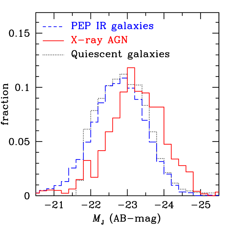
Figure 7: $J$-band absolute magnitude distribution of X-ray AGN (red solid histogram), far-IR selected star-forming galaxies from the PEP survey (blue dashed histogram) and UVJ-selected quiescent galaxies (dotted black histogram) in the redshift interval 0.6-1.4. Rest-frame magnitudes are estimated using k-correct (Blanton & Roweis 2007). For sources with photometric redshifts we use the full PDFs to determine the corresponding $M_{J}$ probability distribution functions, which are then added up to produce the distribution of the entire population.

Figure 8: AGN/galaxy cross-correlation bias, $b_{CCF}$, as a function of the accuracy of the AGN photometric redshifts, parametrised by the dispersion $\sigma_{\Delta z/(1+z)}$. The spectroscopic redshifts of X-ray AGN in the C-COSMOS survey field are convolved with a Gaussian filter of dispersion $\sigma_{\Delta z/(1+z)}$. The resulting PDFs are then cross-correlated with the photometric redshift PDFs of galaxies in the C-COSMOS survey

6 Conclusions

We present a novel method for determining the projected correlation function of extragalactic populations that uses photometric redshift PDFs and is least dependent on spectroscopy. We explore the performance of the method in the case of the X-ray AGN projected cross-correlation function with galaxies. We argue that sample sizes at least 10 times larger than spectroscopic ones are needed to recover the clustering signal at the same level of accuracy. This requires photometric redshifts accurate at a level better than $\sigma_{\Delta z/(1+z)}\approx 0.04$ for both AGN and galaxies. Larger AGN photometric redshift errors, e.g. $\sigma_{\Delta z/(1+z)}\approx 0.08$, require a galaxy sample with photometric redshift dispersion better than $\sigma_{\Delta z/(1+z)}\approx 0.01$. These requirements place constraints on follow-up photometric programmes of future large-area X-ray surveys, such as the eROSITA All Sky Survey. Using the projected cross-correlation function with galaxies, we compare the clustering properties of X-ray AGN, far-IR selected star-forming galaxies and passive systems in the AEGIS-XD and C-COSMOS surveys. It is found that each of the three populations live in dark matter haloes with similar mean masses, $M_{DMH}/(M_{\odot}\,h^{-1})\approx 13.0$. We argue that this is because the galaxies in the three samples have similar stellar mass distributions, approximated by $J$-band luminosity. We hence, conclude that the mean clustering properties of X-ray AGN are determined by the stellar mass of their hosts. We further speculate that claimed trends between AGN properties, such as accretion luminosity or level of obscuration, may be driven by differences in the stellar mass of AGN hosts.

7 Acknowledgments

The authors are grateful to the anonymous referee for helpful comments, M. Krumpe for discussions that improved this paper, J. Aird for providing optical identifications of X-ray sources and O. Ilbert for making available photometric redshift Probability Distribution Functions for galaxies in the COSMOS survey field. GM acknowledges financial support from the Marie-Curie Reintegration Grant PERG03-GA-2008-230644 and the thales project 383549, which is jointly funded by the European Union and the Greek Government in the framework of the programme “Education and lifelong learning”. PGP-G acknowledges support from the Spanish Programa Nacional de Astronomía y Astrofísica under grant AYA2012-31277 This work has made use of the Rainbow Cosmological Surveys Database, which is operated by the Universidad Complutense de Madrid (UCM), partnered with the University of California Observatories at Santa Cruz (UCO/Lick,UCSC). Funding for the DEEP2 Galaxy Redshift Survey has been provided in part by NSF grants AST95-09298, AST-0071048, AST-0071198, AST-0507428, and AST-0507483 as well as NASA LTSA grant NNG04GC89G. Funding for the DEEP3 Galaxy Redshift Survey has been provided by NSF grants AST-0808133, AST-0807630, and AST-0806732. Based on observations obtained with MegaPrime/MegaCam, a joint project of CFHT and CEA/DAPNIA, at the Canada-France- Hawaii Telescope (CFHT) which is operated by the National Research Council (NRC) of Canada, the Institut National des Sciences de l’Univers of the Centre National de la Recherche Scientifique (CNRS) of France, and the University Hawaii. This work is based in part on data products produced at TERAPIX and the Canadian Astronomy Data Centre as part of the Canada-France- Hawaii Telescope Legacy Survey, a collaborative project of NRC and CNRS.

Appendix A Testing the performance of the generalised clustering estimator

The generalised clustering estimation methodology is tested in the AEGIS-XD field, where extensive spectroscopy for both galaxies and AGN is available. This allows comparison with the classic approach of clustering determination that uses only spectroscopic redshift information. Fig. 9, 10 presents the results of this comparison for the galaxy auto-correlation function and the AGN/galaxy cross-correlation function.

A total of 6,500 spectroscopic DEEP2 and DEEP3 galaxies with $R<24.1$ mag in the redshift interval $0.6-1.4$ are used to determine the projected galaxy auto-correlation function. The results are plotted in Figure 9. Then, the DEEP2/DEEP3 spectroscopic sample is replaced with 23,000 CFHTLS-D3 galaxies with $R<24.1$ mag and photometric redshift PDFs (Coupon et al., 2009). These galaxies are selected to have similar redshifts as the spectroscopic subsample by applying the $B-R$ and $R-I$ colour cuts defined by Newman et al. (2012) to pre-select galaxies at $z\ga 0.6$. As a result the CFHTLS-D3 photometric redshift galaxy sample has similar properties (i.e. redshift and luminosity range) to DEEP2/DEEP3 spectroscopic sources. The auto-correlation function of those galaxies is determined using the methodology described above and is plotted in Figure 9. We estimate a galaxy bias of $b=1.63^{+0.07}_{-0.05}$ for the spectroscopic DEEP2/DEEP3 sample (6,500 sources) and $b=1.72^{+0.24}_{-0.15}$ for the 23,000 CFHTLS-D3 photometric galaxies. The uncertainties are estimated for $N_{JK}=8$ Jackknife regions and are 3–4 times larger for the CFHTLS-D3 photometric galaxy sample compared to the spectroscopic sample. This is to be expected since the generalised clustering methodology that uses photometric redshifts only is geared toward large samples. Under the assumption that the bias uncertainty, at a fixed galaxy magnitude limit, scales as $\sqrt{N_{gal}}$ (see Discussion section), we estimate that a sample with size 10 times larger than CFHTLS-D3 is needed to measure the clustering properties of galaxies at the same level of accuracy as the DEEP2/DEEP3 spectroscopic sample. We caution that this calculation does not include the impact of cosmic variance in the error budget.

We further combine the DEEP2/DEEP3 spectroscopic galaxy sample in the range $0.6<z<1.4$ in the AEGIS-XD field with a total of 148 spectroscopic X-ray AGN in the same redshift interval to estimate the projected cross-correlation function. The result is shown in Figure 10. The spectroscopic redshifts of the X-ray AGN are then replaced by their corresponding photometric redshift PDFs and the projected cross-correlation function with the photometric redshift PDFs of the 23 000 CFHTLS-D3 galaxies is estimated. Fig. 10 compares the resulting signal with that obtained using the spectroscopic subsamples. The new method, that uses photometric redshifts only, recovers the clustering signal, but, as expected, the uncertainties are larger. The AGN/galaxy bias is $b=1.72^{+0.12}_{-0.14}$ for the spectroscopic sample and $b=1.84^{+0.40}_{-0.38}$ when replacing the AGN and galaxy spectroscopy with photometric redshift PDFs ($N_{JK}=8$ Jackknife regions).

In the calculations above we adopt $\pi_{max}=50$ Mpc for the classic cross-correlation and auto-correlation functions, based on spectroscopy only. In the case of the generalised clustering estimator that uses photometric redshift PDFs, $\pi_{max}=450$ and 700 Mpc for the cross- and auto-correlation functions, respectively (see Figures 4, 5).

Finally, we emphasize that the methodology described in section 3 is necessary for an unbiased determination of the clustering properties of extragalactic populations using photometric redshifts. Using the photometric redshift best-fit solution underestimates the clustering signal. Fig. 9 demonstrates this point for the auto-correlation function of galaxies in the AEGIS-XD field. The photometric redshift PDFs of galaxies are replaced by the the photometric redshift best-fit solutions and are treated as spectroscopic redshifts. The classic approach of estimating the correlation function is then adopted. In this case the resulting signal (open circles in Figure 9) is systematically underestimated. Similar conclusions apply to the cross-correlation function between X-ray AGN and galaxies. In Figure 10 we also plot the projected cross-correlation function estimated by replacing the photometric redshift PDFs of both galaxies and X-ray AGN with the photometric redshift best-fit solutions. These are then treated as spectroscopic redshifts and the classic approach of estimating the correlation function is adopted (black open circles in Figure 10). This approach underestimates the clustering, although not at the same level of amplitude as in Figure 9.

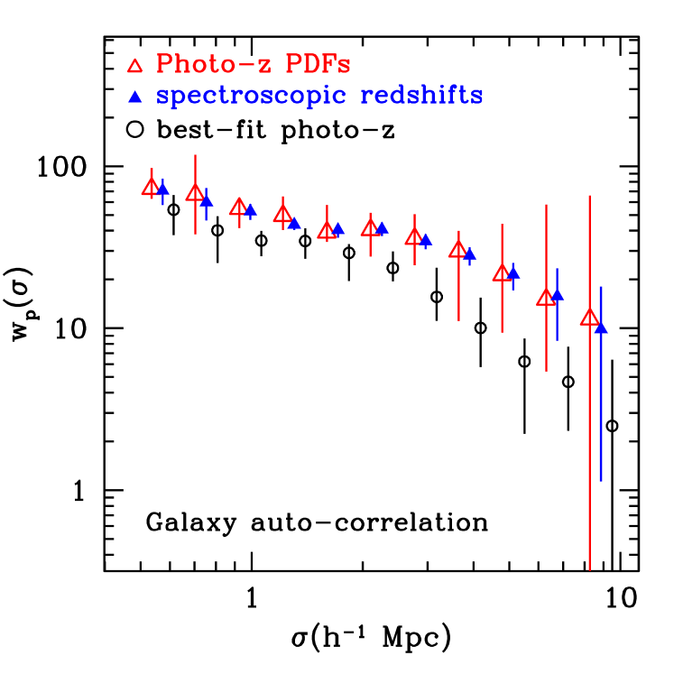
Figure 9: Projected auto-correlation function of galaxies plotted as a function of scale. The filled (blue) triangles correspond to the $\rm w_{p}(\sigma)$ of spectroscopic galaxies selected from the DEEP2 and DEEP3 surveys of the AEGIS field with $R<24.1$ and redshifts in the range $0.6-1.4$. The open (red) triangles are estimated by applying the generalised clustering estimator described in section 3 to the photometric redshift PDFs of CFHTLS-D3 galaxies. The open (black) circles correspond to the auto-correlation $\rm w_{p}(\sigma)$ of the same sample of CFHTLS-D3 galaxies estimated by replacing the photometric redshift PDFs with a single value, the photometric redshift best-fit solution, and then treating them as spectroscopic redshifts in the clustering analysis. The galaxy sample used to estimate the black open circles and the red open triangles is selected to have $R<24.1$ and the optical colour cuts proposed by Newman et al. (2012) to exclude galaxies below $z\approx 0.6$. As a result, the photometrically selected CFHTLS-D3 galaxy sample used in the analysis has similar properties (i.e. redshift and optical luminosity distributions) to DEEP2/3 spectroscopic galaxies. The errorbars are estimated using $N_{JK}=8$ Jackknife regions. For the shake of clarity the open red triangles and black circles are offset in the horizontal direction by $\rm\Delta\log\sigma=-0.02$ and $+0.02$ respectively.

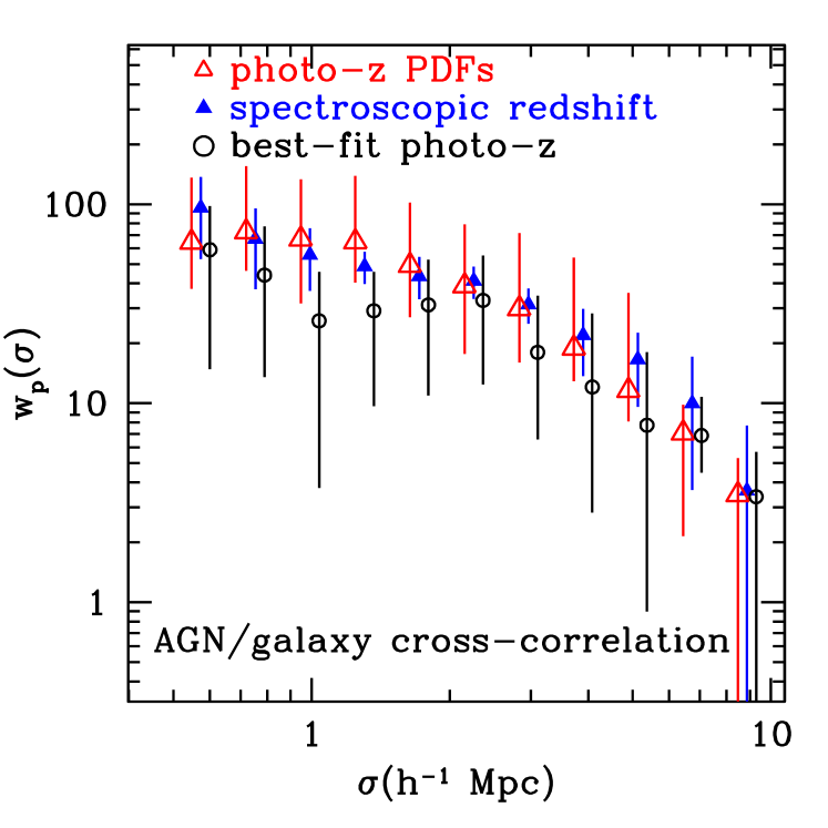
Figure 10: Projected cross-correlation function between X-ray AGN and galaxies plotted as a function of scale. The filled (blue) triangles correspond to the classic approach of estimating the cross-correlation signal, which requires spectroscopy for both samples. Spectroscopic X-ray AGN in the AEGIS-XD field (total of 148) are correlated with DEEP2 and DEEP3 spectroscopic galaxies ($\approx 6,500$) in the same field. The redshift range of both samples is limited to $0.6-1.4$. The open (red) triangles are the projected cross-correlation function estimated by applying the generalised clustering estimator described in section 3. The spectroscopic redshifts of the 148 X-ray AGN in the AEGIS-XD field are replaced by their corresponding photometric redshift PDFs. These are then correlated with the photometric redshift PDFs of 23,000 CFHTLS-D3 galaxies with $R<24.1$ and the optical colour cuts proposed by Newman et al. (2012) to exclude galaxies below $z\approx 0.6$. The open (black) circles correspond to the cross-correlation $\rm w_{p}(\sigma)$ of the same sample of X-ray AGN and CFHTLS-D3 galaxies estimated by replacing the photometric redshift PDFs with a single value, the photometric redshift best-fit solution, and then treating them as spectroscopic redshifts in the clustering analysis. The errorbars are estimated using $N_{JK}=8$ Jackknife regions. For the shake of clarity the open red triangles and black circles are offset in the horizontal direction by $\rm\Delta\log\sigma=-0.02$ and $+0.02$ respectively.

References

- Aird et al. (2012) Aird J., Coil A. L., Moustakas J., Blanton M. R., Burles S. M., Cool R. J., Eisenstein D. J., Smith M. S. M., Wong K. C., Zhu G., 2012, ApJ, 746, 90
- Aird et al. (2013) Aird J., Coil A. L., Moustakas J., Diamond-Stanic A. M., Blanton M. R., Cool R. J., Eisenstein D. J., Wong K. C., Zhu G., 2013, ApJ, 775, 41
- Aird et al. (2010) Aird J., et al., 2010, MNRAS, 401, 2531
- Allevato et al. (2011) Allevato V., et al., 2011, ArXiv 1105.0520
- Allevato et al. (2012) —, 2012, ApJ, 758, 47
- Barro et al. (2011a) Barro G., Pérez-González P. G., Gallego J., Ashby M. L. N., Kajisawa M., Miyazaki S., Villar V., Yamada T., Zamorano J., 2011a, ApJS, 193, 13
- Barro et al. (2011b) —, 2011b, ApJS, 193, 30
- Bell & de Jong (2001) Bell E. F., de Jong R. S., 2001, ApJ, 550, 212
- Bell et al. (2003) Bell E. F., McIntosh D. H., Katz N., Weinberg M. D., 2003, ApJS, 149, 289
- Bielby et al. (2013) Bielby R. M., Gonzalez-Perez V., McCracken H. J., Ilbert O., Daddi E., Le Fèvre O., Hudelot P., Kneib J.-P., Mellier Y., Willott C., 2013, ArXiv 1310.2172
- Brusa et al. (2010) Brusa M., et al., 2010, ApJ, 716, 348
- Bundy et al. (2006) Bundy K., Ellis R. S., Conselice C. J., Taylor J. E., Cooper M. C., Willmer C. N. A., Weiner B. J., Coil A. L., Noeske K. G., Eisenhardt P. R. M., 2006, ApJ, 651, 120
- Bundy et al. (2008) Bundy K., et al., 2008, ApJ, 681, 931
- Calzetti et al. (2000) Calzetti D., Armus L., Bohlin R. C., Kinney A. L., Koornneef J., Storchi-Bergmann T., 2000, ApJ, 533, 682
- Capak et al. (2007) Capak P., et al., 2007, ApJS, 172, 99
- Chary & Elbaz (2001) Chary R., Elbaz D., 2001, ApJ, 556, 562
- Cisternas et al. (2011) Cisternas M., et al., 2011, ApJ, 726, 57
- Coil et al. (2009) Coil A. L., Georgakakis A., Newman J. A., Cooper M. C., Croton D., Davis M., Koo D. C., Laird E. S., Nandra K., Weiner B. J., Willmer C. N. A., Yan R., 2009, ApJ, 701, 1484
- Cooper et al. (2011) Cooper M. C., et al., 2011, ApJS, 193, 14
- Cooper et al. (2012) —, 2012, MNRAS, 419, 3018
- Coupon et al. (2009) Coupon J., et al., 2009, A&A, 500, 981
- Davis & Peebles (1983) Davis M., Peebles P. J. E., 1983, ApJ, 267, 465
- Davis et al. (2007) Davis M., et al., 2007, ApJ, 660, L1
- de la Torre et al. (2011) de la Torre S., et al., 2011, MNRAS, 412, 825
- Elvis et al. (2009) Elvis M., et al., 2009, ApJS, 184, 158
- Fanidakis et al. (2012) Fanidakis N., Baugh C. M., Benson A. J., Bower R. G., Cole S., Done C., Frenk C. S., Hickox R. C., Lacey C., Del P. Lagos C., 2012, MNRAS, 419, 2797
- Fanidakis et al. (2013) Fanidakis N., et al., 2013, ArXiv e-prints 1305.2200
- Foucaud et al. (2010) Foucaud S., Conselice C. J., Hartley W. G., Lane K. P., Bamford S. P., Almaini O., Bundy K., 2010, MNRAS, 406, 147
- Georgakakis et al. (2008) Georgakakis A., Nandra K., Laird E. S., Aird J., Trichas M., 2008, MNRAS, 388, 1205
- Georgakakis et al. (2009) Georgakakis A., et al., 2009, MNRAS, 397, 623
- Georgakakis et al. (2011) —, 2011, MNRAS, 418, 2590
- Hickox et al. (2013) Hickox R. C., Mullaney J. R., Alexander D. M., Chen C.-T. J., Civano F. M., Goulding A. D., Hainline K. N., 2013, ArXiv e-prints 1306.3218
- Hickox et al. (2009) Hickox R. C., et al., 2009, ApJ, 696, 891
- Hickox et al. (2011) —, 2011, ApJ, 731, 117
- Hickox et al. (2012) —, 2012, MNRAS, 421, 284
- Hütsi et al. (2014) Hütsi G., Gilfanov M., Sunyaev R., 2014, A&A, 561, A58
- Ilbert et al. (2009) Ilbert O., et al., 2009, ApJ, 690, 1236
- Kauffmann & Heckman (2009) Kauffmann G., Heckman T. M., 2009, MNRAS, 397, 135
- Kocevski et al. (2012) Kocevski D. D., et al., 2012, ApJ, 744, 148
- Kolodzig et al. (2013) Kolodzig A., Gilfanov M., Hütsi G., Sunyaev R., 2013, A&A, 558, A90
- Komiya et al. (2013) Komiya Y., Suda T., Fujimoto M., 2013, ArXiv e-prints 1312.5069
- Koutoulidis et al. (2013) Koutoulidis L., Plionis M., Georgantopoulos I., Fanidakis N., 2013, MNRAS, 428, 1382
- Krumpe et al. (2010) Krumpe M., Miyaji T., Coil A. L., 2010, ApJ, 713, 558
- Krumpe et al. (2013) —, 2013, ArXiv e-prints, 1308.5976
- Krumpe et al. (2012) Krumpe M., Miyaji T., Coil A. L., Aceves H., 2012, ApJ, 746, 1
- Laird et al. (2009) Laird E. S., et al., 2009, ApJS, 180, 102
- Li et al. (2006) Li C., Kauffmann G., Jing Y. P., White S. D. M., Börner G., Cheng F. Z., 2006, MNRAS, 368, 21
- Lilly et al. (2009) Lilly S. J., et al., 2009, ApJS, 184, 218
- Lutz et al. (2011) Lutz D., et al., 2011, A&A, 532, A90
- Magliocchetti et al. (2011) Magliocchetti M., et al., 2011, MNRAS, 416, 1105
- Magliocchetti et al. (2013) —, 2013, MNRAS, 433, 127
- Magnelli et al. (2009) Magnelli B., Elbaz D., Chary R. R., Dickinson M., Le Borgne D., Frayer D. T., Willmer C. N. A., 2009, A&A, 496, 57
- McCracken et al. (2010) McCracken H. J., et al., 2010, ApJ, 708, 202
- Meneux et al. (2008) Meneux B., et al., 2008, A&A, 478, 299
- Merloni et al. (2012) Merloni A., et al., 2012, ArXiv e-prints1209.3114
- Mostek et al. (2012) Mostek N., Coil A. L., Moustakas J., Salim S., Weiner B. J., 2012, ApJ, 746, 124
- Mountrichas & Georgakakis (2012) Mountrichas G., Georgakakis A., 2012, MNRAS, 420, 514
- Mountrichas et al. (2013) Mountrichas G., Georgakakis A., Finoguenov A., Erfanianfar G., Cooper M. C., Coil A. L., Laird E. S., Nandra K., Newman J. A., 2013, MNRAS, 430, 661
- Mullaney et al. (2012) Mullaney J. R., et al., 2012, MNRAS, 419, 95
- Myers et al. (2009) Myers A. D., White M., Ball N. M., 2009, MNRAS, 399, 2279
- Nandra & Pounds (1994) Nandra K., Pounds K. A., 1994, MNRAS, 268, 405
- Newman et al. (2012) Newman J. A., et al., 2012, ArXiv e-prints, 1203.3192
- Patel et al. (2012) Patel S. G., Holden B. P., Kelson D. D., Franx M., van der Wel A., Illingworth G. D., 2012, ApJ, 748, L27
- Pérez-González et al. (2008) Pérez-González P. G., et al., 2008, ApJ, 675, 234
- Rosario et al. (2012) Rosario D. J., et al., 2012, A&A, 545, A45
- Rosario et al. (2013) —, 2013, ArXiv e-prints 1302.1202
- Rovilos et al. (2012) Rovilos E., et al., 2012, A&A, 546, A58
- Salvato et al. (2009) Salvato M., et al., 2009, ApJ, 690, 1250
- Salvato et al. (2011) —, 2011, ApJ, 742, 61
- Santini et al. (2009) Santini P., Fontana A., Grazian A., Salimbeni S., Fiore F., Fontanot F., Boutsia K., Castellano M., Cristiani S., de Santis C., Gallozzi S., Giallongo E., Menci N., Nonino M., Paris D., Pentericci L., Vanzella E., 2009, A&A, 504, 751
- Santini et al. (2012) Santini P., et al., 2012, A&A, 540, A109
- Schawinski et al. (2010) Schawinski K., et al., 2010, ApJ, 711, 284
- Scoville et al. (2007) Scoville N., et al., 2007, ApJS, 172, 1
- Shao et al. (2010) Shao L., et al., 2010, A&A, 518, L26+
- Sheth et al. (2001) Sheth R. K., Mo H. J., Tormen G., 2001, MNRAS, 323, 1
- Sutherland & Saunders (1992) Sutherland W., Saunders W., 1992, MNRAS, 259, 413
- Trump et al. (2009) Trump J. R., et al., 2009, ApJ, 696, 1195
- van den Bosch (2002) van den Bosch F. C., 2002, MNRAS, 331, 98
- Williams et al. (2009) Williams R. J., Quadri R. F., Franx M., van Dokkum P., Labbé I., 2009, ApJ, 691, 1879
- Zheng et al. (2009) Zheng X. Z., Bell E. F., Somerville R. S., Rix H., Jahnke K., Fontanot F., Rieke G. H., Schiminovich D., Meisenheimer K., 2009, ApJ, 707, 1566