Sensitivity coefficients to $\alpha$-variation for astrophysically relevant transitions in Ni II

Abstract

We calculated the dependence of the transition frequencies on the fine-structure constant $\alpha$ ($q$-factors) for Ni II. Nickel is one of the few elements with high sensitivity to $\alpha$-variation, whose lines are observed at high redshifts. This makes it a sensitive probe for $\alpha$-variation on the cosmological timescale. The electronic structure of Ni II ion was treated within the configuration interaction (CI) method using Dirac-Coulomb Hamiltonian.

I Introduction

There are two dimensionless constants, the fine-structure constant ($\alpha$) and the proton-electron mass ratio ($\mu$), for which spectroscopy is a test ground to probe temporal and spatial variations. The constant $\alpha$ is important for electronic structure of atoms and molecules. The dependence of the spectrum on $\alpha$ appears through the relativistic corrections, such as the fine-structure, Lamb shift, etc. The leading relativistic corrections scale as $\alpha^{2}Z^{2}$ where $Z$ is atomic number. Therefore, heavier elements have higher sensitivity to $\alpha$-variation. For the astrophysically relevant elements $Z<30$ and relativistic corrections do not exceed few percent. The constant $\mu$ enters atomic spectra only through the isotope shifts which are typically on the order of $10^{-3}$, or less. Due to the presence of the vibrational and rotational structures, the dependence of the molecular spectra on $\mu$ is much more pronounced. Therefore, the search for $\alpha$-variation is usually done using atomic spectra Dzuba et al. (1999a, b); Webb et al. (1999); Levshakov et al. (2007); Webb et al. (2011); Molaro et al. (2013); Songaila and Cowie (2014), while $\mu$-variation is studied with the help of molecular spectra Thompson (1975); King et al. (2011); Wendt and Molaro (2012); Rahmani et al. (2013); Albornoz Vásquez et al. (2014); Bagdonaite et al. (2014). Let us note in passing that much higher sensitivity to the variation of both fundamental constants than in optics, can be found in the infrared and microwave wavebands Levshakov et al. (2012); Kozlov and Levshakov (2013).

Astronomical differential measurements of the constant $\alpha$ is based on the comparison of the line centers in the absorption or emission spectra of cosmic objects and the corresponding laboratory values. It follows that the uncertainties of the laboratory rest frequencies and of the line centers in astronomical spectra are the prime concern of such measurements. For example, the unknown isotopic abundances of the elements in the Universe can lead to the systematic frequency shifts, comparable to the expected signal from $\alpha$-variation Kozlov et al. (2004). That is why it is important to use such heavy elements as Fe and Ni where relativistic effects are larger, while isotopic shifts are suppressed.

Most studies of the possible $\alpha$-variation at the redshifts $z\gtrsim 1$ are based on the analysis of the quasar absorbtion spectra using many multiplet method suggested in Refs. Dzuba et al. (1999a, b); Webb et al. (1999). This method utilizes lines of different ions from the same source. All these lines are analyzed simultaneously to find the redshift and the value of $\alpha$ for this object. The lines with small sensitivity coefficients to $\alpha$-variation serve as anchors which give the redshift, while the lines with high sensitivity serve as probes, which give the value of $\alpha$. All lines of the light ions, like Mg II and Al II, belong to the first category. Most lines of heavier ions, like Fe II, Ni II, and Zn II, fall into second category. However, some of the lines of Ni II have relatively small sensitivity and belong to anchors. This can be important for the control of the systematics. The lines of the ion Fe II have sensitivity coefficients to $\alpha$-variation of different signs. This also allows effective control of the possible systematic effects.

At present there is one group, that reports nonzero space-time variation of $\alpha$ on the level of few parts per million (ppm) Webb et al. (2011) (known as the “Australian dipole”). These results have not been confirmed by other groups, who give only upper limits on the $\alpha$-variation also at the ppm level (see Levshakov et al. (2007); Rahmani et al. (2012); Molaro et al. (2013); Songaila and Cowie (2014) and references therein). Because of that it is important to continue observations and include more sources and additional lines. Such programs are currently going on at the VLT and Keck telescopes Molaro et al. (2013); Songaila and Cowie (2014).

A list of the astrophysically relevant optical lines of atoms and ions is given in compilations Berengut et al. (2010); Murphy and Berengut (2013). These compilations includes eleven lines of Ni II. According to Rahmani and Srianand (2013) there are nine lines of Ni II, which can be observed in the quasar spectra including one line not listed in Berengut et al. (2010); Murphy and Berengut (2013). The rest frequencies for Ni II are tabulated in NIST database NIST . Compilation by Morton (2003) includes both frequencies and oscillator strengths $f_{\mathrm{osc}}$ for astrophysically relevant lines. Several high accuracy laboratory rest frequencies were measured in Ref. Pickering et al. (2000). According to Murphy and Berengut (2013) more accurate laboratory measurements are needed. The sensitivity to $\alpha$-variation ($q$-factors) was theoretically studied in Refs. Murphy et al. (2001); Dzuba et al. (2002) for four lines from the list Rahmani and Srianand (2013). In this paper we do calculations of the $q$-factors and oscillator strengths $f_{\mathrm{osc}}$ for all nine astrophysically interesting lines of Ni II.

II Theory and Method

Supposing that the nowadays value of $\alpha$ differs from its value in the earlier Universe we can study space-time variation of $\alpha$ by comparing atomic frequencies for distant objects in the Universe with their laboratory values. In practice, we need to find relativistic frequency shifts, known as $q$-factors Dzuba et al. (1999b, a, 2001, 2003). The difference between the transition frequencies in astrophysical spectra and the laboratory ones is given by the formula:

$$\omega_{i}= \omega_{i}^{(0)}+\omega_{i}^{(2)}\alpha^{2}+\ldots=\omega_{i,\mathrm{lab}}+q_{i}x+\ldots,$$ (1)

$$\omega_{i,\mathrm{lab}}=\omega_{i}^{(0)}+\omega_{i}^{(2)}\alpha_{0}^{2},$$

$$x=(\alpha/\alpha_{0})^{2}-1,\quad q=\partial\omega/\partial x\Bigr{|}_{x=0},$$

where $\omega^{(0)}$ is a transition frequency in non-relativistic approximation, $\omega^{(2)}$ is a relativistic correction. In Eq. (1) $\omega_{i,\mathrm{lab}}$ is the frequency value for $\alpha=\alpha_{0}$, where $\alpha_{0}$ is fine-structure constant in the laboratory (present time) conditions. Note that transition $q$-factor is simply a difference between $q$-factors of upper and lower levels.

For the search of the $\alpha$-variation it is most advantageous to use atoms and ions for which $q$-factors of transitions between certain states significantly differ from each other. That means we need elements with high $Z$. At the same time these elements should be abundant in the Universe to provide sufficient observational data. The latter restriction leaves us with Fe and Ni as the most heavy abundant elements. Fe has been studied in detail in Refs. Porsev et al. (2007); Dzuba and Flambaum (2008); Porsev et al. (2009) and other relevant elements have been studied in Berengut et al. (2004, 2005, 2006); Dzuba and Johnson (2007); Savukov and Dzuba (2008). Ni has been investigated in a lesser detail Dzuba et al. (2002); Murphy et al. (2001) and not all levels observed in astrophysics have been calculated. This is why we return to this problem here.

Rough estimates of the $q$-factors can be obtained from a simple one-particle model Dzuba et al. (1999a). But in order to obtain more accurate values one has to account for electronic correlations and perform large-scale numerical calculations. To find $q$-factors numerically we need to solve the atomic relativistic eigenvalue problem for different values of $\alpha$, or equivalently for different values of $x$ from Eq. (1). In this case we can get $q$-factor as:

$$q\approx\frac{\omega(x_{+})-\omega(x_{-})}{x_{+}-x_{-}}\,.$$ (2)

Our previous experience shows that convenient choice is $x_{\pm}=\pm\tfrac{1}{8}$. In order to test the accuracy of this approximation we can also estimate the second derivative:

$$\left.\frac{\partial^{2}\omega}{\partial x^{2}}\right|_{x=0}=\left.\frac{\partial q}{\partial x}\right|_{x=0}\approx 4\frac{\omega(x_{+})-2\omega(x_{0})+\omega(x_{-})}{(x_{+}-x_{-})^{2}},$$ (3)

where $x_{0}=\tfrac{x_{+}+x_{-}}{2}=0$.

When second derivative (3) is small, results of the calculation using Eq. (2) are sufficiently reliable. If this were not the case we would have strong interaction between levels. Such situation requires more carefulness. It may be useful to trace the levels to smaller values of $x$. Therefore, we do additional calculation for $x=-\tfrac{3}{8}$. When theoretical splitting for the interacting levels at $x=0$ is close to the experimental one, then we can expect good accuracy for the $q$-factors even for this case. Otherwise, if the splitting at $x=0$ differs from the experiment, the $q$-factors calculated for $x=0$ may be incorrect. We can try to improve calculated $q$-factors by moving along $x$ axis to the point where theoretical splitting matches experiment Dzuba et al. (2002). As an additional test of the accuracy of our theory we compare calculated $g$-factors with the experimental ones from NIST .

Absorption spectra in astrophysics correspond to the transitions from the ground state, which in the case of Ni II has $J=5/2$ and belongs to configuration [Ar]$3d^{9}$. Since Ni II has nine electrons in the open shells its spectrum is dense and complicated NIST . Due to the proximity of the levels with the same total angular momentum $J$ and parity $P$ they may strongly interact with each other, in particular for the high frequencies which are more interesting for astrophysics. Because of the selection rules for the transitions from the ground state we are interested in the states of the negative parity with $J=3/2,5/2,7/2$.

In the frequency range observed in the high redshift astrophysics (i.e. roughly between 52000 and 70000 cm^-1) Pickering et al. (2000); Rahmani et al. (2012) there are five lowest odd levels with $J=3/2$, eight levels with $J=5/2$, and seven levels with $J=7/2$. All these levels belong to configurations $3d^{8}4p$, $3d^{7}4s4p$, and $3d^{7}4p4d$. We performed calculations for all these levels, as well as for the ground state for four values of $x$ and found transition frequencies. Then we used cubic interpolation for the interval $0.625<(x+1)<1.275$.

We use Dirac-Coulomb Hamiltonian in the no-pair approximation. Breit corrections to the $q$-factors were studied previously and were found to be small Porsev et al. (2009). We apply configuration interaction (CI) method in the final basis set of relativistic orbitals. All calculations are done with the computer package of I. I. Tupitsyn Bratsev et al. (1977); Kotochigova and Tupitsyn (1987).

We start with solving the Hartree-Fock-Dirac equations. The self-consistency procedure is done for the ground state configuration [Ar]$3d^{9}$. After that all these shells are frozen. The valence orbital $4s$ is constructed for the $3d^{8}4s$ configuration. Then two $4p_{j}$ orbitals are found for the non-relativistic configuration $3d^{8}4p$. On the next stage we make virtual orbitals using the method described in Bogdanovich (1991); Kozlov et al. (1996). In this method an upper component of the virtual orbitals is formed from the previous orbital of the same symmetry by multiplication with some smooth function of radial variable $r$ in the spherical cavity with a radius 50 a.u. The lower component is then formed using kinetic balance condition. This way we make finite basis set of 33 orbitals that include $l=0,\ldots,3$ partial waves ($8spd6f$).

The configuration space is formed by making single and double (SD) excitations from the small list of reference configurations. For even states this list includes $3d^{9}$ and $3d^{8}4s$. For odd states the reference configurations are: $3d^{8}4p$, $3d^{7}4s4p$, and $3d^{7}4p4d$. This way we get 3292 even and 2991 odd relativistic configurations. The number of configurations accounted for in our present calculations is significantly bigger than in the previous calculations in Ref. Dzuba et al. (2002).

Table 1: Results of the calculations for Ni II. Transition frequencies $\omega$, $q$-factors, and $\partial q/\partial x$ are given in cm^-1. Our final recommended values with the errors in brackets are given in the column $q_{\mathrm{recom}}$. In addition to the calculated $g$-factors we give their values in the pure $LS$-coupling scheme. Experimental frequencies and $g$-factors are taken from Ref. NIST . Letters A — H mark the levels which interact in pairs (see discussion in the text). Asterisks mark the lines of prime astrophysical interest.

		Experiment		Theory						Ref.Dzuba et al. (2002)
		$\omega$	$\quad g$	$\omega$	$\quad g_{calc}$	$\quad g(LS)$	$q$	$\partial q/\partial x$	$q_{\mathrm{recom}}$	$q$
${{}^{4}}D_{7/2}$		51558	$1.420$	49002	$1.423$	$1.429$	$\quad-2487$	$-159$	$-2490\,(150)$	$-2415$
${{}^{4}}D_{5/2}$		52739	$1.365$	50239	$1.359$	$1.371$	$-1290$	$-240$	$-1290\,(150)$	$-1231$
${{}^{4}}D_{3/2}$		53635	$1.186$	51183	$1.187$	$1.200$	$-313$	$-179$	$-310\,(150)$
${{}^{4}}G_{7/2}$		54263	$1.025$	51693	$1.010$	$0.984$	$-1393$	$-394$	$-1390\,(150)$	$-1361$
${{}^{4}}G_{5/2}$		55019	$0.616$	52482	$0.609$	$0.571$	$-473$	$-359$	$-470\,(150)$	$-394$
${{}^{4}}F_{7/2}$		55418	$1.184$	53008	$1.194$	$1.238$	$-1181$	$-211$	$-1180\,(150)$	$-1114$
${{}^{4}}F_{5/2}$		56075	$0.985$	53728	$0.996$	$1.029$	$-409$	$-44$	$-410\,(150)$	$-333$
${{}^{2}}G_{7/2}$	A	56371*	$0.940$	53972	$0.923$	$0.889$	$-134$	$-873$	$-250\,(300)$	$-124$
${{}^{4}}F_{3/2}$		56425	$0.412$	54140	$0.420$	$0.400$	$-137$	$-370$	$-140\,(150)$
${{}^{2}}F_{7/2}$	B	57081*	$1.154$	54817	$1.134$	$1.143$	$-969$	$1358$	$-790\,(300)$	$-700(250)$
${{}^{2}}D_{5/2}$	C	57420*	$1.116$	55315	$1.100$	$1.200$	$-1495$	$-200$	$-1500\,(150)$	$-1400(250)$
${{}^{2}}F_{5/2}$	D	58493*	$0.946$	56376	$0.966$	$0.857$	$-98$	$271$	$-100\,(150)$	$-20(250)$
${{}^{2}}D_{3/2}$		58706*	$0.795$	56770	$0.799$	$0.800$	$-367$	$-51$	$-370\,(150)$
${{}^{4}}P_{5/2}$		66571*	$1.480$	66169	$1.506$	$1.600$	$-2205$	$-346$	$-2210\,(150)$
${{}^{4}}P_{3/2}$	E	66580	$1.550$	66173	$1.592$	$1.733$	$-2286$	$-370$	$-2290\,(250)$
${{}^{2}}F_{5/2}$		67695	$0.960$	67512	$0.943$	$1.029$	$-1904$	$-161$	$-1900\,(150)$
${{}^{2}}F_{7/2}$	G	68131*	$1.200$	67921	$1.186$	$1.143$	$-1664$	$-376$	$-1600\,(200)$
${{}^{2}}D_{3/2}$	F	68154*	$1.020$	68080	$1.033$	$0.800$	$-1091$	$120$	$-1090\,(250)$
${{}^{2}}D_{5/2}$		68736*	$1.264$	68753	$1.242$	$1.200$	$-410$	$-332$	$-410\,(150)$
${{}^{4}}D_{7/2}$	H	70778	$1.385$	70704	$1.383$	$1.429$	$-662$	$530$	$-750\,(200)$

III Results and Discussions

Results of our calculations of the energies, $g$-factors, $q$-factors, and their derivatives $\partial q/\partial x$ for the odd levels are presented in Table 1 and Fig. 1. Calculations were done for four values of $x$: $x=-\tfrac{3}{8},-\tfrac{1}{8},\,0,+\tfrac{1}{8}$. Then we did cubic interpolation for the interval $-\tfrac{3}{8}\leq x\leq+\tfrac{1}{8}$. The $q$-factors were found by using Eq. (2) and by differentiation of the interpolation polynomial at $x=0$. Both results appeared to be very close.

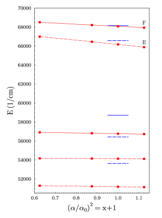
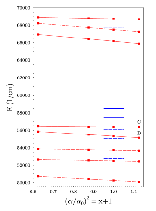
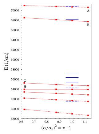
Figure 1: The dependence of the transition frequencies from the ground state on the parameter $(\alpha/\alpha_{0})^{2}=x+1$. Left panel corresponds to $J=3/2$, central panel — $J=5/2$, and right panel — $J=7/2$. The solid lines correspond to the transitions of astrophysical interest, dashed lines — to other transitions. The theoretical curves are obtained by cubic interpolation between marked points. The short horizontal lines indicate experimental data from Ref. NIST . The $q$-factors correspond to the slopes of the curves at $\alpha=\alpha_{0}$.

Identification of the levels is done by comparison of the calculated $g$-factors with the experimental ones and with the prediction of the $LS$-coupling scheme (see Table 1). For the energy range in question the order of the calculated levels agrees with the experiment. Moreover, one can see from the figure that our calculation in general reproduces the splittings between the nearest levels, but somewhat underestimates the energies of the lower levels of negative parity.

For most levels the derivative $\partial q/\partial x$ is rather small and negative. That means that interaction between neighboring levels with the same quantum numbers $J^{P}$ is not very strong. However there are four levels in Table 1 with $\partial q/\partial x>0$. In each of these cases there is close level with large negative $\partial q/\partial x$. Therefore, we can assume that these levels are at pseudo crossing and there is strong repulsion between them. Such interacting pairs of levels are marked on Fig. 1. Below we analyze each of these pairs separately.

Levels A$({}^{2}G_{7/2})$ and B$({}^{2}F_{7/2})$.

This is the strongest interacting pair of levels with $\tfrac{\partial q_{A}}{\partial x}$=$-873\,$cm^-1 and $\tfrac{\partial q_{B}}{\partial x}$=$1358\,$cm^-1. Calculated energy splitting, 845 cm^-1, is larger than experimental splitting 709 cm^-1. It is clear from Fig. 1 that pseudo crossing takes place at positive values of $x$. Both calculated $g$-factors differ from the experiment by roughly 2%. If we move along $x$ axis towards the crossing point at $x=x^{*}\approx 0.28$ we get smaller splitting and can expect better agreement with the experiment. Indeed, the splitting for $x=\tfrac{1}{8}$ is 758 cm^-1, which is almost three times closer to the experimental value. The error for $g$-factors also decreases to 1%, or so. We conclude that this way we do get better agreement with the experiment.

At the pseudo crossing $x=x^{*}$ the levels are parallel to each other, so $q_{A}^{*}=q_{B}^{*}$. Therefore, the shift towards $x^{*}$ strongly affects calculated $q$-factors of each level leaving their sum almost constant. At $x=\tfrac{1}{8}$ we get $q_{A}=-255$ cm^-1 and $q_{B}=-792$ cm^-1. To get exactly experimental splitting we need to move even closer to $x^{*}$. However, the interaction of the levels A and B with other levels is not at all negligible and we need to reproduce other energy splittings as well. This can not be done with the help of the single parameter $x$. Therefore, we take $q$ factors at $x=\tfrac{1}{8}$ as our recommended values. Theoretical error here is, of course, quite large. We estimate it to be around 300 cm^-1, which covers the whole range of $x$ between $x=0$ and $x=x^{*}$.

Levels C$({}^{2}D_{5/2})$ and D$({}^{2}F_{5/2})$.

These levels interact much weaker than the first pair with $\tfrac{\partial q_{C}}{\partial x}$=$-200\,$cm^-1 and $\tfrac{\partial q_{D}}{\partial x}$=$271\,$cm^-1. Besides, the calculated energy splitting, 1061 cm^-1, is very close to the experimental splitting 1073 cm^-1. One of the two $g$-factors is 2% larger than experimental value, but another one is much closer. We conclude that no correction is necessary for this pair of levels.

Levels E$({}^{4}P_{3/2})$ and F$({}^{2}D_{3/2})$.

Though these levels have derivatives of the opposite sign, their absolute values differ by a factor of 3. That means that the two level model is not applicable here. The energy splitting is overestimated by 332 cm^-1, or about 20% and $g$-factor of the level E is 3% larger than experimental value. Because of the strong interaction of this pair with other levels we do not introduce any correction, but rather use the shift in $x$ to estimate the error. Experimental splitting is reproduced at $x=-0.3$ where $q$-factors appears to be: $q_{E}=-2140$ cm^-1 and $q_{F}=-1180$ cm^-1. Therefore, we estimate the error to be about 250 cm^-1 for both levels.

Levels G$({}^{2}F_{7/2})$ and H$({}^{4}D_{7/2})$.

Interaction of these two levels is a little stronger than for the pair (C, D) and theoretical energy splitting, 2647 cm^-1 is 135 cm^-1 smaller, than required. Calculated $g$-factors are quite good, but the difference between them is small and we can not use them to estimate the mixing of these levels with each other. The optimal splitting corresponds to $x=-0.14$ where $q_{G}=-1600$ cm^-1 and $q_{H}=-750$ cm^-1. We estimate the error for the $q$-factors to be about 200 cm^-1.

For the remaining levels, which do not form strongly interacting pairs, the slope remains relatively constant. Calculated $q$-factors are, therefore, less sensitive to the details of the calculation. We checked that any shifts along $x$ axis in order to improve energy splittings between neighboring levels do not change $q$-factors by more than 100 cm^-1. Thus, we estimate theoretical error for these $q$-factors to be around 150 cm^-1. Our final recommended values for the $q$-factors with the error bars are listed in Table 1. Approximately half of the levels from this table were studied before in Ref. Dzuba et al. (2002). For all of them we have good agreement between two calculations. At the same time both calculations do not agree with the earlier calculation Murphy et al. (2001).

Table 2: Oscillator strengths $f_{\mathrm{osc}}$ for the transitions considered in this paper. Calculations were done in the length (L) and velocity (V) gauges. Were possible we compare our results with compilation of Morton (2003) and with Ref. Rahmani and Srianand (2013).

	$\omega$	$f_{\mathrm{osc}}$
	cm-1	L-gauge	V-gauge	Ref. Rahmani and Srianand (2013)	Ref. Morton (2003)
${{}^{4}}D_{7/2}$	51558	2.99E-08	9.83E-11
${{}^{4}}D_{5/2}$	52739	5.86E-04	5.72E-04
${{}^{4}}D_{3/2}$	53635	1.35E-05	1.50E-05
${{}^{4}}G_{7/2}$	54263	3.63E-04	3.30E-04
${{}^{4}}G_{5/2}$	55019	6.99E-05	7.33E-05
${{}^{4}}F_{7/2}$	55418	3.55E-03	3.14E-03	7.16E-03
${{}^{4}}F_{5/2}$	56075	5.39E-04	5.33E-04
${{}^{2}}G_{7/2}$	56371*	2.22E-03	1.95E-03	6.22E-03
${{}^{4}}F_{3/2}$	56425	6.13E-05	6.92E-05
${{}^{2}}F_{7/2}$	57081*	2.75E-02	2.53E-02	2.77E-02	2.77E-02
${{}^{2}}D_{5/2}$	57420*	5.05E-02	5.03E-02	4.27E-02	4.27E-02
${{}^{2}}F_{5/2}$	58493*	4.50E-02	4.36E-02	3.24E-02	3.24E-02
${{}^{2}}D_{3/2}$	58706*	1.04E-02	1.06E-02	6.00E-03	6.00E-03
${{}^{4}}P_{5/2}$	66571*	5.24E-03	4.76E-03	6.00E-03
${{}^{4}}P_{3/2}$	66580	4.40E-04	3.12E-04
${{}^{2}}F_{5/2}$	67695	6.94E-04	8.64E-04		9.72E-04
${{}^{2}}F_{7/2}$	68131*	1.02E-02	1.20E-02	9.90E-03	9.90E-03
${{}^{2}}D_{3/2}$	68154*	8.87E-03	8.03E-03	6.30E-03	6.30E-03
${{}^{2}}D_{5/2}$	68736*	3.03E-02	2.87E-02	2.76E-02	3.23E-02
${{}^{4}}D_{7/2}$	70778	3.15E-03	3.59E-03

Oscillator strengths.

Observability of the transitions considered here depends on the respective oscillator strengths $f_{\mathrm{osc}}$. Not all of them are known from the experiment. We calculated E1 transition amplitudes and $f_{\mathrm{osc}}$ in the length (L) and velocity (V) gauges for all transitions from Table 1. Results are summarized in Table 2. For the transitions with $f_{\mathrm{osc}}>10^{-3}$ two calculations agree within 10%. Even for most weaker transitions $10^{-3}>f_{\mathrm{osc}}>10^{-4}$ the agreement is quite good. Only in one case the difference is close to 30%. Usually, for the CI wave functions the difference between amplitudes in L- and V-gauges can be used to estimate the accuracy of the theory. Therefore we expect our results for the transitions with $f_{\mathrm{osc}}>10^{-4}$ to be accurate within 20-30%. Within this error bar our results agree with compilation of experimental and observational results by Morton (2003). The only exception is the line 58706 cm^-1, where our strength is 50% larger than Morton’s.

We also have mostly good agreement with Ref. Rahmani and Srianand (2013). For the line 68736 cm^-1 our values lie between those of Refs. Morton (2003) and Rahmani and Srianand (2013). However, for the lines 55418 and 56371 cm^-1 our results are significantly smaller. In particular, for the potentially interesting line 56371 cm^-1 our strength is three times smaller than in Rahmani and Srianand (2013). This makes observation of this line for the high redshift sources more difficult.

IV Conclusion

To summarize, here we present theoretical $q$-factors for Ni II found with CI method for Dirac-Coulomb Hamiltonian in no-pair approximation. We calculated $q$-factors for several new lines, which had not been studied theoretically before, but were observed in the high redshift quasar spectra. All calculated sensitivities for Ni II are negative. Two new lines have relatively small $q$-factors, around $-400$ cm^-1 and one has $q$-factor, which is one of the largest in absolute value, $q=-2210$ cm^-1. Note, that large difference in sensitivities of individual lines increases sensitivity of the observations to $\alpha$-variation and allows effective control of the systematics.

In comparison to the previous calculations we have significantly increased the CI space. That did not changed results very much and we have good agreement with the most resent calculation Dzuba et al. (2002). We do not think the accuracy can be noticeably improved within CI method: Ni II has 9 electrons in open shells and it is practically impossible to saturate CI space. On the other hand, already present accuracy is sufficient to analyze astrophysical data on the possible $\alpha$-variation.