The weak lensing signal and the clustering of BOSS galaxies II: Astrophysical and Cosmological constraints

Abstract

We perform a joint analysis of the abundance, the clustering and the galaxy-galaxy lensing signal of galaxies measured from Data Release 11 of the Sloan Digital Sky Survey III Baryon Oscillation Spectroscopic Survey (SDSS III-BOSS) in our companion paper, Miyatake et al. (2014). The lensing signal was obtained by using the shape catalog of background galaxies from the Canada France Hawaii Telescope Legacy Survey, which was made publicly available by the CFHTLenS collaboration, with an area overlap of about 105 deg². We analyse the data in the framework of the halo model in order to fit halo occupation parameters and cosmological parameters ($\Omega_{\rm m}$ and $\sigma_{8}$) to these observables simultaneously, and thus break the degeneracy between galaxy bias and cosmology. Adopting a flat $\Lambda$CDM cosmology with priors on $\Omega_{b}h^{2}$, $n_{\rm s}$ and $h$ from the analysis of WMAP 9-year data, we obtain constraints on the stellar mass-halo mass relation of galaxies in our sample. Marginalizing over the halo occupation distribution parameters and a number of other nuisance parameters in our model, we obtain $\Omega_{\rm m}=0.310^{+0.019}_{-0.020}$ and $\sigma_{8}=0.785^{+0.044}_{-0.044}$ (68% confidence). We demonstrate the robustness of our results with respect to sample selection and a variety of systematics such as the halo off-centering effect and possible incompleteness in our sample. Our constraints are consistent, complementary and competitive with those obtained using other independent probes of these cosmological parameters. The cosmological analysis is the first of its kind to be performed at a redshift as high as $0.53$.

1. Introduction

The overwhelming majority of the energy density of the Universe today is dominated by two mysterious components – dark energy and cold dark matter – both motivated by astrophysical observations (see e.g, Ostriker et al., 1974; Rubin et al., 1978; Riess et al., 1998; Perlmutter et al., 1999; Hinshaw et al., 2013; Planck Collaboration et al., 2013a). Since their discovery, the field of observational cosmology has focused on characterizing the precise abundance, the statistical distribution and the phenomenological behaviour of these components. Geometrical probes such as the observations of type-Ia supernovae (see e.g., Lampeitl et al., 2010; Sullivan et al., 2011; Suzuki et al., 2012) and the baryonic acoustic oscillation measurements (see e.g., Eisenstein et al., 2005; Percival et al., 2007a; Blake et al., 2011a; Anderson et al., 2014) have provided constraints on the energy density of various components in the Universe as a function of redshift, but are insensitive to the statistical properties of the dark matter distribution. Probing the latter requires constraints on the growth of structure in the Universe, which can be provided by measurements of the abundance of galaxy clusters (see e.g., Vikhlinin et al., 2009; Mantz et al., 2010; Rozo et al., 2010; Benson et al., 2013; Hasselfield et al., 2013; Planck Collaboration et al., 2013c), redshift space distortions (see e.g., Percival et al., 2004; Beutler et al., 2012; Reid et al., 2014) and the statistics of weak gravitational lensing as a function of redshift (see e.g., Van Waerbeke et al., 2000; Lin et al., 2012; Huff et al., 2014; Heymans et al., 2013; Mandelbaum et al., 2013). Over the next decade, a combination of these probes will enable a phenomenological understanding of the nature of dark energy and dark matter as well as stringent constraints on modifications to gravity (see e.g., Albrecht et al., 2006).

The growth of structure in the Universe is driven by the growth of fluctuations in dark matter, which are easier to describe analytically on large scales (Bernardeau et al., 2002) or via collisionless numerical simulations on small scales (Davis et al., 1985) than the variety of astrophysical processes that baryons undergo in order to form galaxies (see e.g., Springel et al., 2005; Rudd et al., 2008; Vogelsberger et al., 2014). Observationally, however, it is easier to use galaxies to trace out the underlying structure in matter. Since galaxies form within halos, at the peaks of the matter density field, using galaxies as tracers produces a biased view of the matter distribution (Kaiser, 1984). The bias of halos with respect to the matter distribution and its dependence on halo mass can be fortunately predicted given the cosmological parameters within the framework of the standard concordance cosmological model (Bardeen et al., 1986; Mo & White, 1996a; Sheth & Tormen, 1999; Sheth et al., 2001; Tinker et al., 2010).

On large scales the bias of halos and the galaxies that reside in them approaches a constant value. On such scales the shape of the matter two-point function (the power spectrum or the correlation function) can be inferred from the observed galaxy two-point function, and used to constrain cosmological parameters (Tegmark et al., 2004; Percival et al., 2007b; Reid et al., 2010; Saito et al., 2011). However, in the case of the galaxy two-point function, the amplitude of the matter power spectrum, which is essential to study the growth of structure, is entirely degenerate with the value of the bias. The determination of galaxy bias can be complicated as it is known to depend upon the properties of galaxies such as their luminosity and colour (Norberg et al., 2001; Tegmark et al., 2004; Zehavi et al., 2011; Guo et al., 2013), and is quite scale dependent on small scales (Fry & Gaztanaga, 1993; Mann et al., 1998; Cacciato et al., 2012). Nevertheless, this degeneracy between the large scale bias and the amplitude of the matter power spectrum can be broken if there is a way to infer the connection between galaxies and their halo masses (Seljak et al., 2005).

There are a number of different approaches to directly infer the galaxy-dark matter connection. Many different observables can be used to probe this connection, including galactic rotation curves (Rubin, 1983), kinematics of satellite galaxies (Zaritsky et al., 1997; van den Bosch et al., 2004; More et al., 2009b, 2011), small scale redshift space distortions (Hikage et al., 2013; Li et al., 2012), $X$-ray emission from the hot intra-cluster medium (see reviews by Kravtsov & Borgani, 2012; Ettori et al., 2013). However, these methods assume that the system is in dynamical equilibrium, an assumption that is certainly violated in some systems. Weak gravitational lensing provides a way to circumvent this assumption and can be used as a relatively clean probe of the halo masses. In combination with weak lensing, the information encapsulated in the shape and amplitude of the clustering signal can be fully exploited (Seljak et al., 2005; Cacciato et al., 2009; Mandelbaum et al., 2013; Hikage et al., 2013; Cacciato et al., 2013a; More et al., 2013; Reid et al., 2014). This combination can provide simultaneous constraints on the connection between galaxies and dark matter and the cosmological parameters. Cosmological constraints from such studies obtained at different cosmic epochs can then be used to constrain the equation of state of dark energy.

In Miyatake et al. (2013, Paper I hereafter), we measure the large scale clustering of galaxies in the Sloan Digital Sky Survey III (SDSS-III hereafter) Baryon Oscillation Spectroscopic Survey (BOSS hereafter). In particular, we employ the CMASS galaxy sample from BOSS as our parent sample. We use the deep but limited area imaging data from the Canada France Hawaii Telescope Legacy Survey (CFHTLS hereafter), to measure the weak gravitational lensing signal around galaxies from BOSS to calibrate the masses of the halos in which they reside. In this paper, we model these observations simultaneously in the framework of the halo model. We will obtain joint constraints on the astrophysical properties of galaxies in our sample such as their halo occupation distribution, limiting constraints on their stellar masses, and the density profile of dark matter halos in which they reside, as well as cosmological constraints on the matter density parameter $\Omega_{{\rm m}}$ and the amplitude of density fluctuations characterized by the parameter $\sigma_{8}$.

This paper is organized as follows. In Section 2, we introduce the data products used to perform our analysis and briefly describe the measurements of the galaxy clustering and the galaxy-galaxy lensing signal. In Section 3, we present the theoretical background for how these measurements can constrain cosmological parameters and the analytical halo occupation distribution model we use to interpret the data. The results of our main analysis and a variety of systematics tests are presented in Section 4. We conclude in Section 5 with a summary of our results and discuss the outlook for ongoing and future surveys. We will assume a flat $\Lambda$CDM cosmology with $\Omega_{\rm m}=0.27$ when converting redshifts to distances for performing the clustering and lensing measurements. Throughout this paper, $\log$ denotes the $10-$based logarithm of a quantity, the symbols $h$ and $h_{70}$ denote the Hubble constant, $H_{0}$ normalized by $100\>{\rm km}\,{\rm s}^{-1}\,{\rm Mpc}^{-1}$ and $70\>{\rm km}\,{\rm s}^{-1}\,{\rm Mpc}^{-1}$, respectively.

2. Data and Measurements

We use the sample of galaxies compiled in Data Release 11 (DR11) of the SDSS-III project. The SDSS-III is a spectroscopic investigation of galaxies and quasars selected from the imaging data obtained by the SDSS (York et al., 2000) I/II covering about $11,000$ deg² (Abazajian et al., 2009) using the dedicated 2.5-m SDSS Telescope (Gunn et al., 2006). The imaging employed a drift-scan mosaic CCD camera (Gunn et al., 1998) with five photometric bands ($u,g,r,i$ and $z$) (Fukugita et al., 1996; Smith et al., 2002; Doi et al., 2010). The SDSS-III (Eisenstein et al., 2011) BOSS project (Ahn et al., 2012; Dawson et al., 2013) obtained additional imaging data of about 3,000 deg² (Aihara et al., 2011). The imaging data was processed by a series of pipelines (Lupton et al., 2001; Pier et al., 2003; Padmanabhan et al., 2008) and corrected for Galactic extinction (Schlegel et al., 1998) to obtain a reliable photometric catalog. This catalog was used as an input to select targets for spectroscopy (Dawson et al., 2013) for conducting the BOSS survey (Ahn et al., 2012) with the SDSS spectrographs (Smee et al., 2013). Targets are assigned to tiles of diameter $3^{\circ}$ using an adaptive tiling algorithm designed to maximize the number of targets that can be successfully observed (Blanton et al., 2003). The resulting data were processed by an automated pipeline which performs spectral classification, redshift determination, and various parameter measurements, e.g., the stellar mass measurements from a number of different stellar population synthesis codes which utilize the photometry and redshifts of the individual galaxies (Bolton et al., 2012). The galaxy samples in BOSS have been divided into a low redshift LOWZ sample, and a high redshift CMASS galaxy sample. In addition to the galaxies targetted by the BOSS project, we also use galaxies which pass the target selection but have already been observed as part of the SDSS-I/II project (legacy galaxies). These legacy galaxies are subsampled in each sector so that they obey the same completeness as that of the CMASS sample (Anderson et al., 2014). In addition to the above standard reductions, we have also obtained stellar masses for fiber collided galaxies and galaxies with redshift failures using their own photometry but assuming that their redshift is identical to the nearest neighbours .

In order to define subsamples of galaxies we use stellar masses for galaxies obtained using the Portsmouth stellar population synthesis code (Maraston et al., 2013) with the assumptions of a passively evolving stellar population synthesis model and a Kroupa (2001) initial mass function. In Paper I, we divided the parent sample of CMASS galaxies into subsamples in the stellar mass-redshift plane. The three subsamples A, B and C that we use in our analysis all lie in the redshift range $z\in[0.47,0.59]$ and include galaxies in the stellar mass range $\log M_{*}\in[11.10,12.00]$, $\log M_{*}\in[11.30,12.00]$ and $\log M_{*}\in[11.40,12.00]$, respectively. We will denote subsample A to be fiducial, and test the sensitivity of our cosmological constraints to possible incompleteness using the rest of the subsamples. The number of galaxies in subsamples A, B and C are $400,916$, $196,578$ and $116,682$ corresponding to number densities of $3\times 10^{-4}$, $1.5\times 10^{-4}$ and $0.8\times 10^{-4}~{}h^{3}\>{\rm Mpc}^{-3}$, respectively. These numbers include galaxies that were fiber collided and/or had failures in redshift measurements. The number density of galaxies in each of the samples shows much less variation (less than $\sim 20\%$ in the redshift range under consideration) with redshift than the parent sample (see Figure 1 in Paper I).

For the measurements of the galaxy-galaxy lensing signal around the subsamples of CMASS galaxies, we must measure the tangential distortion of background galaxies. For this purpose, we rely on the deeper and better quality imaging data from the Canada France Hawaii Telescope Legacy survey (CFHTLS). This information allows us to measure the tangential distortion of background galaxies around our sample of CMASS galaxies. In particular we make use of the photometric reduction and image shape determinations in the publicly available CFHTLenS catalog. The quantities needed for each galaxy, namely its shear estimate, calibration factors, weight, and photometric redshift are provided in the catalog (Heymans et al., 2012; Erben et al., 2013; Miller et al., 2013; Hildebrandt et al., 2012). Unfortunately, the overlap between the CFHTLS and the DR11 BOSS fields is limited to an area of about 105 deg². The number of CMASS galaxies that lie within the CFHTLS footprint is $5,084$ for our fiducial subsample A, $2,549$ from subsample B and $1,577$ for subsample C , respectively.

In Paper I, we presented measurements of the projected clustering of galaxies, $w_{\rm p}(r_{\rm p})$ for a number of different subsamples of galaxies. At fixed redshift, we detected a clear dependence of the clustering signal on the stellar mass of galaxies. Higher stellar mass galaxies are more clustered than lower stellar mass galaxies. However, we also observed that the clustering of galaxies of fixed stellar mass does not vary significantly with redshift, in particular within the range of redshifts for the 3 subsamples considered in this paper. In Paper I, we also measured the galaxy-galaxy lensing signal around each of our subsamples. We also found the strength of the lensing signal to be larger for higher stellar mass threshold samples, consistent with the expectation that these galaxies reside in higher mass halos. In the next section we develop a simple picture which shows how the joint measurements of clustering and lensing of galaxies can be used to constrain cosmological parameters, as well as present the details of the analytical model we use in order to fit a parametric model to these measurements.

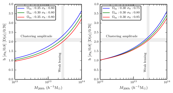
Figure 1.— Theoretical predictions of the amplitude of the galaxy clustering signal on large scales as a function of the halo mass of these galaxies in different cosmological models at $z=0.53$. The left hand panel shows how the clustering amplitude varies when $\Omega_{\rm m}$ is increased, while the right hand panel shows the corresponding change when $\sigma_{8}$ is increased. Measurements of the clustering of galaxies and the galaxy-galaxy lensing signal determine the ordinate and the abscissa, respectively, thus allowing constraints on these cosmological parameters.

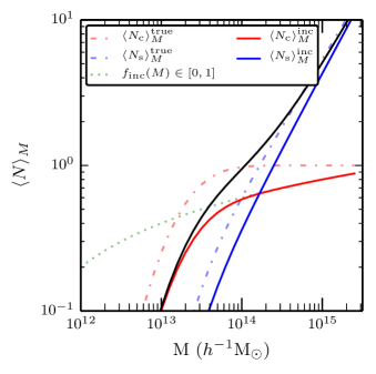
Figure 2.— An illustration of the halo occupation distribution model we use in the analysis of this paper. The red and blue dot-dashed lines show the central and satellite components of the HOD appropriate for a true stellar mass threshold sample. The green dotted line shows the log-linear functional form we assume for parametrizing the incompleteness in our subsample. The solid red, blue and black lines show the HOD of centrals, satellites and all galaxies after accounting for the incompleteness. In total our HOD model is parametrized by 7 parameters.

3. Theory

Structure formation in the concordance $\Lambda$CDM cosmological model occurs as a result of the gravitational collapse of initial density fluctuations into extended halos of dark matter. The abundance of halos in different cosmological models has a universal form when expressed as a function of peak height, $\nu=\delta_{\rm c}/\sigma$, where $\delta_{\rm c}$ is the critical threshold for collapse, $\sigma(M,z)$ is the variance of density fluctuations smoothed on spatial scales corresponding to the comoving radius from which the halo mass $M$ assembled (e.g., Mo & White, 1996b; Sheth & Tormen, 1999). These halos form preferentially at the peaks of the matter density field and hence are biased with respect to the matter distribution. The halo bias can also be expressed as a function of the peak height. Galaxies share the bias of the halos in which they reside. The overall clustering amplitude at sufficiently large separation is determined by the products of this bias ($b$), the amplitude of the linear matter fluctuations ($\sigma_{8}$) and the growth rate of fluctuations at a given redshift ($D(z)$); $w_{\rm p}(r_{\rm p})\propto[b\sigma_{8}D(z)]^{2}$.

Figure 1 displays the dependence of the clustering amplitude of halos as a function of their mass on cosmological parameters at $z=0.53$, the average redshift of our sample. In the left hand panel, $\sigma_{8}$ is fixed while the matter density, $\Omega_{\rm m}$, is varied for flat $\Lambda$CDM cosmological models. In the right hand panel, $\Omega_{\rm m}$ is fixed while $\sigma_{8}$ is varied. Increasing both $\Omega_{\rm m}$ and $\sigma_{8}$ results in a decrease of the clustering amplitude at fixed halo mass. The measurement of the clustering amplitude of galaxies fixes the clustering amplitude of halos in which they reside. However, one can obtain similar clustering amplitudes in different cosmological models by changing the halos in which galaxies reside. This behavior is the classical degeneracy between halo occupation distribution parameters and the cosmological parameters; one can obtain the same clustering amplitude for galaxies by having them reside in larger mass halos in cosmologies with larger $\Omega_{\rm m}$ or $\sigma_{8}$. The weak lensing signal on small scales breaks this degeneracy by direct inference of the mass of the halos, thus allowing a determination of cosmological parameters. Given the errors in determination of the clustering amplitude and the halo mass, we expect degeneracy in the determination of $\Omega_{\rm m}$ and $\sigma_{8}$ such that increasing the value of one can be compensated by decreasing the value of the other.

The above qualitative picture is valid if galaxies occupy a narrow range of halo masses. In reality, in our stellar mass threshold samples, galaxies span a range in halo masses. In addition, although most galaxies are central galaxies in their halos, some of those in our subsample are satellite galaxies. The average clustering amplitude, $A_{\rm gal}$, is related to the bias of halos through an integral over the halo occupation distribution of the galaxies in our subsample,

$$\langle A\rangle_{\rm gal} = \sigma_{8}D(z)b_{\rm eff}$$ (1)

$$= \sigma_{8}D(z)\frac{\int{\rm d}M\langle N\rangle_{M}b(M,z)n(M,z)}{\int{\rm d}M\langle N\rangle_{M}n(M,z)}\,,$$

where the ratio of the integrals is the effective bias ($b_{\rm eff}$) of the galaxy sample. Similarly, the average mass of halos as determined from the weak lensing signal needs to appropriately account for the halo occupation distribution of the galaxies.

3.1. Analytical HOD model

We use a halo occupation distribution model (hereafter HOD; Jing et al., 1998; Peacock & Smith, 2000; Seljak, 2000a; Scoccimarro et al., 2001; Zheng et al., 2005; Leauthaud et al., 2012; van den Bosch et al., 2013; Cacciato et al., 2013a, b), to predict the abundance, the clustering and the lensing signal of CMASS galaxies. We adopt an HOD model with an explicit split of the halo occupation into central and satellite galaxies (see Figure 2),

$$\langle N\rangle_{M}=\langle N_{\rm c}\rangle_{M}+\langle N_{\rm s}\rangle_{M}$$ (2)

The mean halo occupation distribution for central galaxies is given by

$$\langle N_{\rm c}\rangle_{M}=f_{\rm inc}(M)\frac{1}{2}\left[1+{\rm erf}\left(\frac{\log M-\log M_{\rm min}}{\sigma_{\log M}}\right)\right],$$ (3)

and that for satellite galaxies is given by

$$\langle N_{\rm s}\rangle_{M}=\langle N_{\rm c}\rangle_{M}\left[\frac{M-\kappa M_{\rm min}}{M_{1}}\right]^{\alpha}$$ (4)

when $M>\kappa M_{\rm min}$ and zero otherwise (see e.g., Zheng et al., 2005; White et al., 2011). The function $f_{\rm inc}(M)$ accounts for potential incompleteness in the selection of CMASS galaxies at the low stellar mass end (see e.g., More et al., 2011; Reddick et al., 2013) when compared to a true stellar mass threshold sample. We assume a log-linear functional form for the incompleteness function such that

$$f_{\rm inc}(M) = {\rm max}[0,{\rm min}[1,1+\alpha_{\rm inc}(\log M-\log M_{\rm inc})]]$$ (5)

This model explicitly assumes that the CMASS selection selects a random fraction of the stellar mass threshold galaxies, given by $f_{\rm inc}$, from host halos at every mass scale, equivalently, it assumes that with the CMASS color and magnitude cuts, the selection probability for galaxies at a given stellar mass do not depend on the environment or other properties.

We follow the analytical framework developed in van den Bosch et al. (2013) (with a minor extension to account for the miscentering of central galaxies with respect to their halo centers), to predict the galaxy-galaxy clustering and the galaxy-galaxy lensing signal, using the halo occupation distribution described above. We briefly present the key expressions below for completeness.

The galaxy-galaxy power spectrum, $P_{\rm gg}(k,z)$, is the Fourier transform of the galaxy correlation function, $\xi(r,z)$ and can be expressed as a sum of the following one- and two-halo terms,

$$P_{\rm gg}(k,z) = 2\,P^{\rm 1h}_{\rm cs}(k,z)+P^{\rm 1h}_{\rm ss}(k,z)$$ (6)

$$+P^{\rm 2h}_{\rm cc}(k,z)+2\,P^{\rm 2h}_{\rm cs}(k,z)+P^{\rm 2h}_{\rm ss}(k,z)\,.$$

Here the subscripts “${\rm c}$” and “${\rm s}$” stand for central and satellite galaxy, respectively. Each of these terms can be expressed in the following compact form

$$P^{\rm 1h}_{\rm xy}(k,z)=\int{\rm d}M\,{\cal H}_{\rm x}(k,M,z)\,{\cal H}_{\rm y}(k,M,z)\,n(M,z),$$ (7)

$$P^{\rm 2h}_{{\rm x}{\rm y}}(k,z)=\int{\rm d}M_{1}\,{\cal H}_{\rm x}(k,M_{1},z)\,n(M_{1},z)$$ (8)

$$\times\int{\rm d}M_{2}\,{\cal H}_{\rm y}(k,M_{2},z)\,n(M_{2},z)\,Q(k|M_{1},M_{2},z)\,,$$

where ‘x’ and ‘y’ are either ‘c’ (for central) or ‘s’ (for satellite), $n(M,z)$ describes the halo mass function at redshift $z$, $Q(k|M_{1},M_{2},z)$ describes the power-spectrum of haloes of masses $M_{1}$ and $M_{2}$ and accounts for the radial dependence of bias, non-linearities in the matter power spectrum and halo exclusion, ingredients that can be calibrated by numerical simulations (see, e.g., van den Bosch et al., 2013). Furthermore, we have defined

$${\cal H}_{\rm c}(k,M,z)=\frac{\langle N_{\rm c}\rangle_{M}}{\bar{n}_{{\rm g}}(z)}\,\left(1-p_{\rm off}+p_{\rm off}\exp\left[-\frac{1}{2}k^{2}(r_{\rm s}{\cal R}_{\rm off})^{2}\right]\right)\,,$$ (9)

and

$${\cal H}_{\rm s}(k,M,z)=\frac{\langle N_{\rm s}\rangle_{M}}{\bar{n}_{{\rm g}}(z)}\,\tilde{u}_{\rm s}(k|M,z)\,.$$ (10)

Here, we have assumed that there is a fraction $p_{\rm off}$ of central galaxies that are offset from the center of their halos (see e.g., Skibba et al., 2011) and that the normalized radial profile of the off-centered galaxies, with respect to the true halo center, is a Gaussian with width relative to the scale radius, $r_{\rm s}$, of the halo in which they reside,

$$u_{\rm off}(r|M)=\frac{1}{(2\pi)^{3/2}(r_{\rm s}{\cal R}_{\rm off})^{3}}\exp\left[-\frac{1}{2}\left(\frac{r}{r_{\rm s}{\cal R}_{\rm off}}\right)^{2}\right]\,.$$ (11)

The Fourier transform of $u_{\rm off}(r|M)$ is $\exp[-k^{2}(r_{s}{\cal R}_{\rm off})^{2}/2]$, and the quantity $\tilde{u}_{\rm s}(k|M)$ in ${\cal H}_{\rm s}(k,M,z)$ is the Fourier transform of an Navarro-Frenk-White (Navarro et al., 1996, hereafter NFW) profile for a halo of mass $M$ (see also Hikage et al., 2013, for a similar model). We also assume that the normalized number density profile of satellite galaxies follows the NFW profile. The number density of galaxies, $\bar{n}_{{\rm g}}(z)$, is given by

$$\bar{n}_{{\rm g}}(z)=\int\langle N\rangle_{M}n(M,z){\rm d}M$$ (12)

We will assume a $\sim$20 percent fractional error on the abundances, since our stellar mass cuts yield a roughly constant abundance with redshift, with $\sim 20$ percent level fluctuations. In the presence of parameters to model the incompleteness we do not expect the abundances to influence the cosmological constraints in a significant manner.

The real-space correlation function, $\xi_{\rm gg}(r,z)$, can be obtained by an inverse Fourier transform of the galaxy-galaxy power spectrum . We use a modified version of the large scale redshift space distortion model presented by Kaiser (1987) to predict $\xi^{z}_{\rm gg}(r_{\rm p},\pi,z)$ from $\xi_{\rm gg}(r,z)$ (see van den Bosch et al., 2013, for details), and integrate along the line-of-sight,

$$w_{\rm p}(r_{\rm p})=2\int_{0}^{\pi_{\rm max}}\xi(r_{\rm p},\pi)\,{\rm d}\pi\,.$$ (13)

to calculate the projected correlation function. This modified model accounts for residual redshift space distortions on large scales due to finite value of $\pi_{\rm max}$ (see e.g., Norberg et al., 2009; Baldauf et al., 2010; More, 2011; van den Bosch et al., 2013). The upper limit for the line-of-sight integration we adopt is $\pi_{\rm max}=100\>h^{-1}{\rm{Mpc}}$, thus mimicking the integration limit adopted in the measurements in Paper I for the subsamples of galaxies we use.

The galaxy-galaxy lensing signal is a probe of the excess surface density,

$$\Delta\Sigma(r_{\rm p})=\langle\Sigma(<r_{\rm p})\rangle-\bar{\Sigma}(r_{\rm p})\,$$ (14)

The surface density $\Sigma(r_{\rm p},z)$ can be obtained by projecting the galaxy-matter correlation function, $\xi_{gm}(r,z)$, using

$$\Sigma(r_{\rm p},z)=\int_{R}^{\infty}\bar{\rho}\,[1+\xi_{\rm gm}(r,z)]\frac{2\,r\,{\rm d}r}{\sqrt{r^{2}-r_{\rm p}^{2}}}\,.$$ (15)

In order to predict the galaxy-matter cross power spectrum, we adopt the HOD model framework. The cross power spectrum is given by the sum of the following one- and two-halo terms

$$P_{\rm gm}(k,z)=P^{\rm 1h}_{\rm cm}(k,z)+P^{\rm 1h}_{\rm sm}(k,z)+P^{\rm 2h}_{\rm cm}(k,z)+P^{\rm 2h}_{\rm sm}(k,z)\,.$$ (16)

Each of the above terms can be calculated using Eqs. (7)-(8), where ‘x’ is ‘m’ (for matter) and ‘y’ is either ‘c’ (for central) or ‘s’ (for satellite). For the matter component, we define

$${\cal H}_{\rm m}(k,M,z)={M\over\bar{\rho}_{{\rm m}}(z)}\,\tilde{u}_{\rm h}(k|M,z)\,,$$ (17)

where $\tilde{u}_{\rm h}(k|M,z)$ is the Fourier transform of the normalized density distribution of matter within a halo of mass $M$, and $\bar{\rho}_{{\rm m}}(z)$ denotes the average comoving density of the Universe at redshift $z$. The galaxy-matter correlation function can be obtained by an inverse Fourier transform of the galaxy-matter power spectrum.

The lensing signal is sensitive to the total matter content of galaxies including both the dark matter and the baryonic components. Therefore, we will also consider the matter component in the lens galaxy, which includes stars and gas. At distances close to the lensing galaxy, these terms could dominate the lensing signal. We assume that the effect of the matter component in the lens galaxy can be considered as a point mass contribution located at the position of the lens galaxy,

$$\Delta\Sigma_{\ast}(r_{\rm p})=\frac{\tilde{M}_{\ast}}{\pi r_{\rm p}^{2}}\,,$$ (18)

where $\tilde{M}_{\ast}$ is in units of $h^{-1}M_{\odot}$ and the projected radius $r_{\rm p}$ is in units of $h^{-1}\>{\rm pc}$. The stellar population synthesis models (hereafter SPS) infer the stellar mass, $M_{\ast}$ based upon the luminosity and mass-to-light ratio of stars. These masses therefore have the units of $h^{-2}M_{\odot}$, and this stellar mass is related to the baryonic lensing mass by $\tilde{M}_{\ast}=M_{\ast}/h$. Our models adopt the parameter $M_{\ast}$ to allow a comparison of this mass with the stellar mass measurements from the SPS models.

In addition to the HOD parameters, our analytical predictions also depend upon the cosmological parameters, via the halo mass function, the halo bias function, and the cosmology dependence of the concentration-mass relation (van den Bosch et al., 2013). There are a number of simulation-calibrated ingredients required to use the analytical expressions in this section. For the sake of completeness and reproducibility, we list each of them below. We assume the halo masses to be $200$ times overdense with respect to the background matter density. We use the halo mass function calibration of Tinker et al. (2008) and large scale bias calibration of Tinker et al. (2010) for this particular definition. The radial dependence of halo bias was calibrated by Tinker et al. (2005) for friends-of-friends halos. We use an appropriate modification to take into account the spherical overdensity definition of halos and the effects of halo exclusion (see van den Bosch et al., 2013) which allows us to calculate $Q(k|M_{1},M_{2},z)$. We use a nuisance parameter $\psi$ to marginalize over the uncertain description of radial dependence of halo bias. This parameter governs the behaviour of the prediction in the transition regime between one- and two-halo terms (see van den Bosch et al., 2013, for details). The concentration of dark matter halos is assumed to follow the concentration-mass relation calibration presented by Macciò et al. (2008). We allow for a normalization parameter $R_{\rm c}$ which characterizes deviations from this fiducial relation and assign it a prior of $1.00\pm 0.20$. We also assume that the number density profile of satellite galaxies will share the same concentration as that of the dark matter distribution. We have checked that increasing the width of the prior on the $R_{\rm c}$ to $0.30$, or allowing the concentration parameter for satellite galaxy distribution to differ from the dark matter distribution does not significantly affect our results. In addition, we also allow for a $2.5$ percent uncertainty in the modeling of the projected clustering signal (the overall amplitude) to account for the inaccuracies of the model. We do not explicitly include a corresponding systematic uncertainty in the lensing calibration, since the statistical errors on that measurement are already sufficiently large that they are the dominant source of error, compared to the statistical error on the systematic shear calibration correction (Miller et al., 2013).

3.2. Cosmological parameter dependence of the measurements

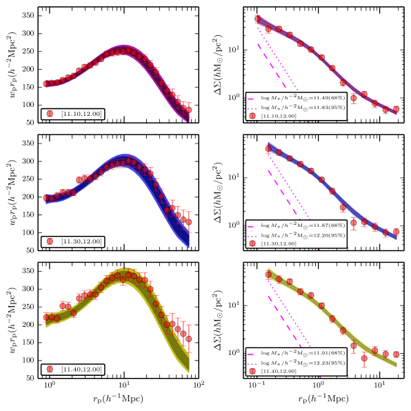
Figure 3.— The 68 and 95 percent confidence intervals of the fits to the clustering measurements (left panels) and the lensing measurements (right panels) obtained from the HOD modeling exercise for subsamples A, B and C are shown in the top, middle and bottom rows, respectively. The intervals are obtained by projecting uncertainties in all the model parameters around the best-fit model. The reduced $\chi^{2}$ for the best fit models in the three cases are $0.8$, $1.3$ and $1.5$ for 31, 31 and 30 degrees of freedom, respectively (see text for details). The 68 and 95 percent upper limits on the stellar mass of galaxies are also shown in the right hand panels.

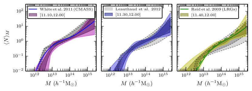
Figure 4.— The 68 and 95 percent confidence intervals of the halo occupation distribution of CMASS galaxies in samples A, B and C obtained from our modeling exercise are shown in the three different panels, respectively. The HOD constraints displayed here are marginalized over the uncertainty in the cosmological parameters. Subsamples A, B and C occupy progressively more massive halos. The results for subsample A can be contrasted with results from White et al. (2011) who constrain the HOD using the clustering of an early data release of CMASS galaxies (shown as solid blue line in left hand panel). The halo occupation distribution for sample C is consistent with the HOD obtained by Reid & Spergel (2009, shown as green solid line in the right hand panel), based on a counts-in-cylinder analysis of the LRG sample of galaxies. The green dashed line in the right hand panel shows the result of a simple attempt to correct for the differences in the mean redshift of LRGs and CMASS galaxies by adjusting the masses of LRGs at $z=0.3$ to the masses of their progenitors at $z=0.53$. The gray shaded bands in each of the subsample show the constraints on the HOD obtained by Leauthaud et al. (2012) from COSMOS data, employing the same stellar mass cuts in the galaxy selection. The similarity of our HOD constraints, especially for the higher stellar mass threshold samples, implies that the magnitude of potential incompleteness effects in our analysis decrease with increasing stellar mass threshold.

The abundance, clustering and the lensing measurements depend upon the fiducial cosmological model, ${\cal C}^{\rm fid}$, that we have assumed to convert the angular and redshift differences in the positions of galaxies to their comoving separation. We follow More (2013), in order to account for this dependence. For a given cosmological model ${\cal C}$, we multiply the predicted abundance of galaxies $\bar{n}_{\rm g}({\cal C})$ in the redshift bin $[z_{2},z_{1}]$ by the ratio of the comoving volumes

$$\bar{n}_{\rm g}^{\prime}=\bar{n}_{\rm g}({\cal C})\frac{\chi^{3}(z_{2},{\cal C})-\chi^{3}(z_{1},{\cal C})}{\chi^{3}(z_{2},{\cal C}^{\rm fid})-\chi^{3}(z_{1},{\cal C}^{\rm fid})}$$ (19)

in order to compare it to abundance measured assuming ${\cal C}^{\rm fid}$. Here, $\chi(z)$ denotes the comoving distance to redshift $z$. For the clustering and the lensing signals, we first calculate $w_{\rm p}$ and $\Delta\Sigma$ at comoving separations $r_{\rm p}^{\prime}$, which are related to the projected comoving separation $r_{\rm p}^{\rm fid}$ at which the measurements were performed by

$$r_{\rm p}^{\prime}=r_{\rm p}^{\rm fid}\left[\frac{\chi(\bar{z},{\cal C})}{\chi(\bar{z},{\cal C}^{\rm fid})}\right]$$ (20)

where $\chi^{\rm fid}$ and $\chi$ denote the comoving distance to the median redshift $\bar{z}$ in ${\cal C}^{fid}$ and ${\cal C}$, respectively. This calculation accounts for the difference in the conversion of angular differences between galaxies to comoving separations. We need to further change the amplitude of the predictions of both $w_{\rm p}$ and $\Delta\Sigma$, such that

$$\tilde{w}_{\rm p}(r_{\rm p})=w_{\rm p}(r_{\rm p}^{\prime})\left[\frac{E(\bar{z})}{E^{\rm fid}(\bar{z})}\right]$$ (21)

$$\tilde{\Delta\Sigma}(r_{\rm p})=\Delta\Sigma(r_{\rm p}^{\prime})\left[\frac{\Sigma_{\rm crit}(\bar{z},z_{\rm s})}{\Sigma_{\rm crit}^{\rm fid}(\bar{z},z_{\rm s})}\right],$$ (22)

where the former equation accounts for the cosmology dependence of the conversion from redshift difference to comoving line-of-sight distances, while the latter corrects for the cosmology dependence of $\Sigma_{\rm crit}$, which is used to calculate the lensing signal from the measured ellipticities. We use a fixed source redshift to calculate $\Sigma_{\rm crit}(\bar{z},z_{\rm s})$ due to its weak dependence on the choice of the source redshift. We compare these modified predictions with the measurements. The validity of this procedure to capture the cosmological dependence of the measurements procedure was verified in More (2013).

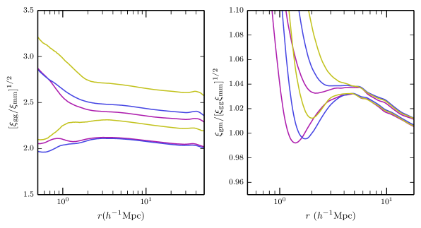
Figure 5.— The 68 percent confidence limits on the scale-dependence of bias (left panel) and the cross-correlation coefficient (right panel) of our subsamples A, B and C are enclosed by the magenta, blue and yellow lines, respectively. The bias tends to a constant value on large scales, and the cross-correlation coefficient shows small but significant deviations from unity at small scales.

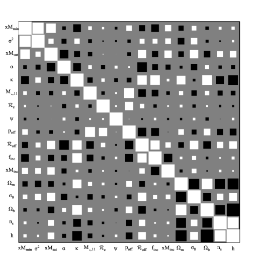
Figure 6.— The degeneracies between different parameters constrained by our modeling of the clustering and lensing of CMASS galaxies with stellar mass threshold $\log M_{*}>11.10$. Positive correlations in the posterior are displayed with white squares and the negative correlations are displayed with black squares. The size of the squares indicates the strength of correlation.

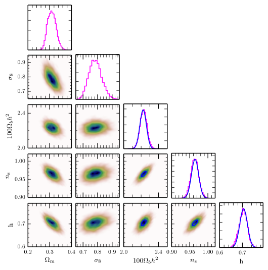
Figure 7.— The degeneracies between different cosmological parameters as inferred from the analysis of the clustering and lensing signal from our fiducial subsample A are shown with shaded contours in the off-diagonal panels. The magenta histograms in the diagonal columns represent the posterior distribution of each of our cosmological parameters. The blue distributions in the diagonal panels and the blue contour (68 percent confidence) in some of the off-diagonal panels represent the prior information we adopt on the parameters $[\Omega_{\rm b}h^{2},n_{\rm s},h]$.

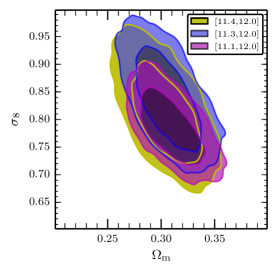
Figure 8.— The constraints in the $\Omega_{\rm m}-\sigma_{8}$ plane obtained from the analysis of the different stellar mass threshold samples are shown using contours of different colours. As the higher stellar mass subsamples are expected to be more complete, this provides a systematic check of the possible bias in our cosmological constraints due to incompleteness.

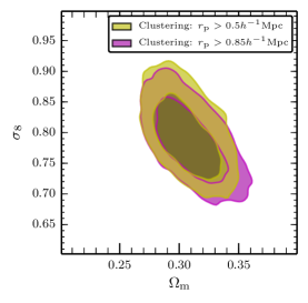
Figure 9.— The constraints in the $\Omega_{\rm m}-\sigma_{8}$ plane obtained from the fiducial subsample A, but restricting the projected clustering signal to different scales. The magenta contours correspond to our fiducial analysis with $r_{\rm p}>0.85\>h^{-1}{\rm{Mpc}}$, while the yellow contours correspond to $r_{\rm p}>0.5\>h^{-1}{\rm{Mpc}}$. Inclusion of the small scale clustering information does not cause a drastic improvement in the cosmological constraints.

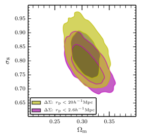
Figure 10.— The constraints in the $\Omega_{\rm m}-\sigma_{8}$ plane obtained from the fiducial subsample A, but restricting the galaxy-galaxy lensing signal to small scales. The magenta contours correspond to our fiducial analysis with $r_{\rm p}<20.0\>h^{-1}{\rm{Mpc}}$, while the yellow contours correspond to $r_{\rm p}<2.6\>h^{-1}{\rm{Mpc}}$. By excluding the large scales, we are less sensitive to the two halo-term in the lensing signal, which could be affected if the CFHTLS sample is not representative of our CMASS subsample.

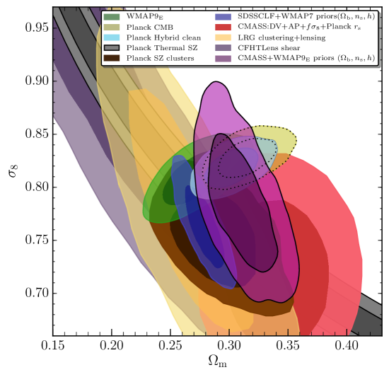
Figure 11.— The 68 and 95 percent confidence constraints on the matter density parameter, $\Omega_{\rm m}$ and the fluctuation amplitude parameter, $\sigma_{8}$ obtained from the analysis of the clustering and lensing measurements of our fiducial sample are shown using magenta contours. These can be compared with results from other cosmological probes such as the analyses of the cosmic microwave background carried out by the WMAP team (green shaded regions, denoted as WMAP$9_{\mbox{E}}$), the Planck team (chrome yellow shaded regions with dotted contours; Planck CMB) and a reanalysis of Planck data by Spergel et al. (2013, light blue shaded regions; Planck Hybrid clean), the SZ cluster abundances (brown shaded regions; Planck SZ clusters) and the thermal SZ power spectrum (gray shaded regions; Planck Thermal SZ) carried out by the Planck team, the joint analysis of clustering and lensing of the SDSS main galaxy sample (dark blue; SDSSCLF+WMAP7) by Cacciato et al. (2013a), and that of the LRG sample (yellow; LRG clustering+lensing) by (Mandelbaum et al., 2013), the joint analysis of redshift space distortions , BAOs and the Alcock Paczynski test using CMASS galaxies (red shaded regions; CMASS:DV+AP+$f\sigma_{8}$+Planck $r_{s}$) by (Beutler et al., 2013) and the tomographic weak lensing signal (violet shaded regions; CFHTLens shear) by (Heymans et al., 2013). The figure shows that our results are consistent, complementary and competitive with constraints from different cosmological probes.

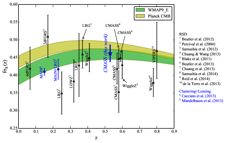
Figure 12.— Blue dots denote $f\sigma_{8}(z)$ constraints calculated from our measurement and other joint analyses of clustering and lensing measurements. Black triangles denote $f\sigma_{8}(z)$ constraints based on various RSD measurements. Some of the RSD CMASS measurements are shifted along the redshift-axis for clarity ($+0.01$ for references 6 and 8 and $+0.02$ for reference 9). Error bars show 68 percent confidence level. Green (Yellow) shaded region shows $f\sigma_{8}$ predictions with 68 percent confidence intervals based on the WMAP9 (Planck) CMB measurement. Our result is the highest redshift cosmological analysis using a joint analysis of the clustering and lensing signal of galaxies.

3.3. Summary of model parameters

The analytical model we use to describe the measurements has 17 parameters. The first set of 5 parameters, $M_{\rm min},\sigma^{2},M_{\rm sat},\alpha,\kappa$, describes the halo occupation distribution of galaxies. The parameter $M_{*,11}$ describes the average stellar mass of galaxies in units of $h^{-2}M_{\odot}$, while ${\cal R}_{\rm c}$ is the normalization of the concentration mass relation with respect to the one obtained from simulations. We have 5 nuisance parameters: $\psi,p_{\rm off},{\cal R}_{\rm off},\alpha_{\rm inc},M_{\rm inc}$. Finally there are 5 cosmological parameters: $\Omega_{\rm m},\sigma_{8},\Omega_{\rm b}h^{2},n_{\rm s}$ and $h$. We let $\Omega_{\rm m}$ and $\sigma_{8}$ be completely free but use priors on the latter three cosmological parameters from the joint likelihood of the cosmic microwave background analysis of the WMAP 9-year data and the high resolution CMB measurements from the South Pole Telescope (SPT) and the Atacama Cosmology Telescope (ACT) obtained by Hinshaw et al. (2013). We will denote this combination of cosmological priors as WMAP9_E. Our samples A and B have 27 measurements of $w_{\rm p}$, 14 measurements of $\Delta\Sigma$ and one of the abundance for the subsample each, used for the analysis. We have 17 total model parameters, with priors on the 3 cosmological parameters $(\Omega_{\rm b}h^{2},n_{\rm s},h)$ and on the 3 parameters $\alpha,{\cal R}_{\rm c},\psi$. Therefore, the total number of degrees of freedom are $27+14+1-17+6=31$. The number of degrees of freedom are 30 for subsample C which does not include the innermost bin in the lensing measurement. We perform a Bayesian inference of cosmological parameters given the measurements using a Markov chain Monte Carlo (hereafter MCMC) analysis. In particular, we use the affine invariant sampler of Goodman & Weare (2010) as implemented by the software emcee to navigate the parameter space (Foreman-Mackey et al., 2013).

4. Results

We now present the results of our HOD analysis and the different systematic tests we have performed. The 68 percent confidence intervals on each of our parameters from the analysis of the abundance, clustering and the lensing signal of the three stellar mass subsamples we use are listed in Table 4. The top left- and right-hand panels of Figure 3 show the projected clustering data and the lensing data with errorbars for the fiducial subsample of galaxies, while the middle and bottom panels display the corresponding results for subsamples B and C, respectively. The dark and light colored shaded regions denote the 68 and 95 percent confidence intervals obtained from the MCMCs, respectively, marginalizing over all of the model parameters. The overall shape of the clustering and lensing signals is reproduced well by the model. The clustering and lensing predictions are able to successfully reproduce the increasing strength with stellar mass thresholds, as in the observations. The model is also able to reproduce the shape of the weak lensing signal and the observed transition between the one- and two-halo regimes. There is a hint that the model has some difficulty reproducing the high amplitude of the clustering on large scales for the higher stellar mass threshold samples. However, note that the large scales have significant covariance. The reduced $\chi^{2}$ for the best fit models for the fiducial subsample is $0.8$, while those of the subsamples B and C are $1.3$ and $1.5$, respectively. The probabilities to exceed the $\chi^{2}$ values by chance given the number of degrees of freedom are equal to $76\%$, $10\%$ and $4\%$, respectively.

The right hand panels of Figure 3 present the 68 and 95 percent upper limits on the average stellar mass of the galaxies in each subsample using dashed and dotted lines, respectively. The 68 percent confidence limits from the weak lensing modeling are $\langle M_{*}\rangle<3\times 10^{11}h^{-2}M_{\odot}$, $\langle M_{*}\rangle<7.4\times 10^{11}h^{-2}M_{\odot}$ and $\log\langle M_{*}\rangle<8.1\times 10^{11}h^{-2}M_{\odot}$ for the progressively larger stellar mass subsamples, respectively. These limits on the average stellar masses from weak lensing have been marginalized over uncertainties in the cosmological model. We compare our results with the estimates of stellar masses for our subsample of galaxies from stellar population synthesis models with a variety of different assumptions and codes in Table 2. The limits could be improved in the near future if the weak lensing signal can be measured to even smaller scales (Kobayashi et al., submitted). We expect such measurements to potentially constrain stellar population synthesis models.

Table 1Posterior distribution of parameters from the MCMC analysis

		Subsample
Parameter	[11.10,12.00]	[11.30,12.0]	[11.40,12.0]
$\log M_{\rm min}$	$13.13_{-0.13}^{+0.13}$	$13.45_{-0.15}^{+0.15}$	$13.68_{-0.16}^{+0.16}$
$\sigma^{2}$	$0.22_{-0.15}^{+0.14}$	$0.45_{-0.25}^{+0.24}$	$0.79_{-0.39}^{+0.41}$
$\log M_{1}$	$14.21_{-0.13}^{+0.11}$	$14.51_{-0.15}^{+0.17}$	$14.56_{-0.22}^{+0.27}$
$\alpha$	$1.13_{-0.45}^{+0.38}$	$1.14_{-0.51}^{+0.47}$	$1.00_{-0.43}^{+0.45}$
$\kappa$	$1.25_{-0.69}^{+0.71}$	$0.85_{-0.67}^{+0.67}$	$1.19_{-0.96}^{+0.99}$
$M_{*,11}$	$0.0^{+3.1}$	$0.0^{+7.3}$	$0.0^{+8.1}$
${\cal R}_{\rm c}$	$0.98_{-0.20}^{+0.19}$	$1.01_{-0.20}^{+0.20}$	$1.02_{-0.22}^{+0.21}$
$\psi$	$0.93_{-0.13}^{+0.14}$	$0.93_{-0.14}^{+0.15}$	$0.94_{-0.14}^{+0.15}$
$p_{\rm off}$	$0.34_{-0.18}^{+0.18}$	$0.37_{-0.21}^{+0.24}$	$0.36_{-0.19}^{+0.19}$
${\cal R}_{\rm off}$	$2.2_{-1.3}^{+1.5}$	$2.3_{-1.5}^{+1.5}$	$2.4_{-1.4}^{+1.4}$
$\alpha_{\rm inc}$	$0.44_{-0.34}^{+0.35}$	$0.53_{-0.24}^{+0.25}$	$0.57_{-0.18}^{+0.20}$
$\log M_{\rm inc}$	$13.57_{-0.30}^{+0.32}$	$13.88_{-0.30}^{+0.33}$	$14.08_{-0.29}^{+0.32}$
$\Omega_{\rm m}$	$0.310_{-0.020}^{+0.019}$	$0.306_{-0.020}^{+0.021}$	$0.304_{-0.021}^{+0.022}$
$\sigma_{8}$	$0.785_{-0.044}^{+0.044}$	$0.839_{-0.061}^{+0.061}$	$0.813_{-0.059}^{+0.060}$
$100\Omega_{\rm b}h^{2}$	$2.228_{-0.040}^{+0.040}$	$2.226_{-0.039}^{+0.040}$	$2.222_{-0.041}^{+0.041}$
$n_{\rm s}$	$0.964_{-0.011}^{+0.011}$	$0.963_{-0.010}^{+0.011}$	$0.961_{-0.011}^{+0.011}$
$h$	$0.703_{-0.018}^{+0.018}$	$0.700_{-0.016}^{+0.017}$	$0.695_{-0.017}^{+0.017}$

The three columns list the $68\%$ confidence intervals on the model parameters for the three stellar mass subsamples we use in our analysis. The parameter $M_{{}_{*},11}$ denotes the stellar mass in units of $10^{11}~{}h^{-2}M_{\odot}$ and the $68\%$ limit we quote is a one-sided upper limit.

Table 2Population synthesis models average stellar masses

	Subsample A	Subsample B	Subsample C
Model	$\langle M_{\ast}\rangle$ $(10^{11}\,h^{-2}M_{\odot})$	$\langle M_{\ast}\rangle$ $(10^{11}\,h^{-2}M_{\odot})$	$\langle M_{\ast}\rangle$ $(10^{11}\,h^{-2}M_{\odot})$
Portsmouth Passive Kroupa	1.14	1.51	1.79
Portsmouth Star-forming Kroupa	0.97	1.28	1.53
Portsmouth Passive Salpeter	1.95	2.55	2.96
Portsmouth Star-forming Salpeter	1.51	1.99	2.38
Granada Early-forming dust Kroupa	3.07	3.72	4.18
Granada Late-forming dust Kroupa	2.59	3.11	3.46
Granada Early-forming nodust Kroupa	2.58	3.13	3.53
Granada Late-forming nodust Kroupa	2.19	2.62	2.95
Granada Early-forming dust Salpeter	5.09	6.18	6.93
Granada Late-forming dust Salpeter	4.33	5.19	5.79
Granada Early-forming nodust Salpeter	4.33	5.25	5.93
Granada Late-forming nodust Salpeter	3.67	4.41	4.96
Our model	$<3.0$ (68%)	$<7.4$ (68%)	$<8.1$ (68%)

The average stellar mass estimate for the subsamples of galaxies used to measure the clustering and lensing of galaxies in the present study from different SPS models. The sample was defined using the first of these models, and the same sample was used to estimate the average stellar mass in all cases. For comparison, our $68\%$ model constraints are listed in the bottom two rows for the fiducial and the off-centering model, respectively.

The constraints on the halo occupation distribution for the three samples are shown in Figure 4. As expected, the HOD shifts to higher halo masses for subsamples B and C. The scatter in halo masses increases significantly for the highest threshold sample. A constant scatter in stellar masses at fixed halo mass translates into an increasing scatter in halo masses at fixed stellar mass due to the shallow power law index of the stellar mass halo mass relation at the massive end (see e.g., More et al., 2009a). We compare our HOD constraints to those obtained by White et al. (2011) for the full sample of CMASS galaxies in the left hand panel of Figure 4. Compared to their sample, our fiducial subsample of galaxies resides in slightly larger halo masses owing to our subsample selection which removes low stellar mass galaxies. Next we compare the HOD of our subsample C to that of luminous red galaxies (LRGs) from SDSS-I/II at $z\sim 0.3$. These two samples have comparable number densities. In the right hand panel, we compare the HOD constraints with those obtained by Reid & Spergel (2009) for luminous red galaxies shown with solid line. The comparison demonstrates the similarity in the HOD of the two samples. For reference, we also show the HOD of LRGs shifted to adjust for the difference in the mass of the halos owing to the difference in the average redshift of the LRG sample ($z\sim 0.3$) and that of our subsample ($z\sim 0.53$). This particular HOD should hold if all LRGs have both maintained their identities (central or satellite) inside their respective halos and if none of these halos merged with each other in the redshift interval $z\in[0.35,0.57]$.

We also compare our HOD constraints with results obtained by Leauthaud et al. (2012) with a similar analysis of the abundance, clustering and lensing signal but with data from the COSMOS survey. The gray shaded regions in each of the panels of Figure 4 show the 68 and 95 percent confidence intervals obtained using the parameter constraints from Leauthaud et al. (2012), for the same stellar mass cut as our selection in each panel . The COSMOS sample covers a much smaller area on the sky but is expected to be more stellar mass complete compared to the CMASS sample, which has color cuts designed to select the luminous red galaxy population. The comparison shows that the galaxies in the fiducial subsample on average reside in slightly larger halo masses than the results from COSMOS. This result is consistent with the expectation that massive redder galaxies reside in higher mass halos on average (see e.g., More et al., 2011). The results for subsamples B and C are, however, consistent with the results from COSMOS, implying that the incompleteness in our subsamples becomes smaller for the larger stellar mass thresholds. As the blue fraction of galaxies decreases steeply as a function of stellar mass, the CMASS colour selection no longer biases the sample. Tinker et al. (in preparation) demonstrate this trend of decreasing incompleteness with increasing stellar mass threshold in the CMASS sample based on galaxies that did not pass the CMASS colour cuts but were observed as part of an SDSS-III ancillary program (J. Tinker, priv. comm.).

The clustering and lensing signals of satellite galaxies are different from that of central galaxies on small scales. Therefore it is important to obtain a good estimate on the fraction of galaxies that are satellites in our subsamples in order to correctly interpret the measurements. The satellite fraction of our fiducial subsample is $8.3\pm 3.1$ percent. This value is consistent with the satellite fraction quoted by White et al. (2011), $10\pm 2$ percent, albeit on the lower side. This is not entirely unexpected as our subsample excludes the low stellar mass galaxies in the entire CMASS sample that was used by White et al. (2011). The satellite fraction is expected to decrease as a function of stellar mass. The satellite fractions in our higher stellar mass threshold subsamples are $6.8\pm 2.6$ and $4.6\pm 2.1$, respectively, consistent with this expectation.

With the large flexibility in our modeling, we obtain very weak constraints on the off-centering parameters, $p_{\rm off}$ and ${\cal R}_{\rm off}$. We also do not detect any significant deviation of the concentration-mass relation from the assumed relation calibrated from numerical simulations. We have observed that when the off-centering parameters are not included, the posterior distribution of ${\cal R}_{\rm c}$ shifts to lower values (by about 20 percent). A similar magnitude offset in the concentration-mass relation was also observed by Mandelbaum et al. (2008) by analyzing the weak lensing signal (whilst ignoring the off-centering issue) on a wider range of mass scales, from MaxBCG clusters (Koester et al., 2007), LRGs, and $L_{\ast}$ lens (Mandelbaum et al., 2006).

The large-scale effective bias of galaxies (defined as in Equation 1) of our fiducial subsample of galaxies is constrained to be $2.15\pm 0.13$. This value is in agreement with the bias value of $2.05\pm 0.3$ inferred by Comparat et al. (2013) using the angular clustering and weak lensing of all CMASS galaxies that were flagged as potential spectroscopic targets in the CFHT Stripe 82 region. The galaxy bias systematically increases to $2.26\pm 0.17$ and $2.54\pm 0.19$, respectively, for subsamples with progressively larger stellar mass thresholds. In the left hand panel of Figure 5, we show the scale dependence of the bias defined as

$$b(r)=\left[\frac{\xi_{\rm gg}(r)}{\xi_{\rm mm}(r)}\right]^{1/2}\,,$$ (23)

where $\xi_{\rm gg}$ and $\xi_{\rm mm}$ are the three dimensional galaxy and matter correlation functions, respectively. The magenta, blue and yellow lines enclose the 68 percent confidence intervals for our subsamples A, B and C after marginalizing over all of our model parameters, respectively. The right hand panel shows the cross-correlation coefficient defined as

$$r_{\rm ccc}(r)=\frac{\xi_{\rm gg}(r)}{\left[\xi_{\rm mm}(r)\xi_{\rm gm}(r)\right]^{1/2}}\,,$$ (24)

where $\xi_{\rm gm}(r)$ is the three dimensional galaxy-matter cross-correlation. This is a prediction based on the HOD models allowed by the data. This prediction is consistent with the value of $r_{\rm ccc}(r)=1.16\pm 0.35$ measured by Comparat et al. (2013) averaged on scales of $0.1$–$2\>h^{-1}{\rm{Mpc}}$. The cross-correlation coefficient is larger than one on small scales (see e.g., Seljak, 2000b), but tends to unity on large scales. This behaviour of the cross-correlation coefficient on large scales can be used to obtain the matter correlation function directly from observations of the galaxy clustering and galaxy-galaxy lensing on large scales (Seljak, 2000b; Guzik & Seljak, 2001; Baldauf et al., 2010; Cacciato et al., 2012; Mandelbaum et al., 2013).

In Figure 6, we present the different degeneracies that are inherent to our analysis. Large white (black) squares indicate positive (negative) correlations in the inferred parameters. The scatter in halo masses, $\sigma^{2}$, is tightly correlated with the mass scale, $M_{\rm min}$, above which halos host one central galaxy. This degeneracy is expected due to the dependence of each of the observables on these two parameters. Increasing $M_{\rm min}$ results in increasing the mean halo mass of galaxies (and also the galaxy bias relevant for the large scale clustering). However, one can compensate for this increase by increasing the scatter, and thereby including more lower mass halos. The off-centering parameters are degenerate with each other and show weak degeneracies with the satellite galaxy parameters and the incompleteness parameters. In the case of a large off-centering fraction, we expect the central signal to mimic the satellite signal which can explain the degeneracies we observe. The cosmological parameters, $\Omega_{\rm m}$ and $\sigma_{8}$ are degenerate with each other (see Section 3), and show degeneracies with the other cosmological parameters, which we will discuss shortly. However, more importantly, $\Omega_{\rm m}$ and $\sigma_{8}$ show only weak degeneracies with other HOD parameters. This separation of degeneracies between the cosmological parameters and the HOD parameters is a useful feature of the joint analyses of the clustering and lensing of galaxies (More et al., 2013).

We show the posterior distributions of our cosmological constraints as histograms in the diagonal panels of Figure 7 for our fiducial subsample. The shaded regions highlight the degeneracies between the cosmological parameters. The distributions shown by the blue solid lines denote the priors that we have assumed on the auxiliary cosmological parameters $\Omega_{\rm b}h^{2},n_{\rm s}$ and $h$ based on the analysis of WMAP9+SPT+ACT (Hinshaw et al., 2013). There is no significant improvement on these parameters with the addition of our data, neither does our data shift the posteriors of these parameters away from the priors (cf. Cacciato et al., 2013a). We also observe the degeneracy in the constraints on $\Omega_{\rm m}$ and $\sigma_{8}$ that we anticipated from our theoretical considerations: a larger value of $\Omega_{\rm m}$ prefers a model with smaller value of $\sigma_{8}$ as implied from Figure 1.

The cosmological constraints on $\Omega_{\rm m}$ and $\sigma_{8}$ obtained from the three stellar mass subsamples analysed in this paper are depicted in Figure 8 with magenta, blue and yellow contours, respectively. The constraints from our higher threshold subsamples, which are expected to be more complete, are consistent with the fiducial subsample. Thus, although the fiducial subsample may have been incomplete, this incompleteness does not cause significant biases in the cosmological constraints, compared to the current statistical precision. Given that the HOD for each of the subsamples differs significantly from each other, this agreement is non-trivial.

In our analysis, we have analysed the measurements of clustering to $r_{\rm p}>0.85\>h^{-1}{\rm{Mpc}}$. We tested for additional systematics by extending our measurements to even smaller scales $r_{\rm p}>0.5\>h^{-1}{\rm{Mpc}}$, but restrict ourselves above the fiber collision scale at the highest redshift of our subsamples. The small-scale clustering signal is sensitive to the satellite fraction, and thus our constraints are expected to marginally improve. The 68 and 95 percent confidence levels on $\Omega_{\rm m}-\sigma_{8}$ for such an analysis of our fiducial subsample are compared to those obtained when analyzing the larger scale measurements in Figure 9. This test also does not reveal any significant biases.

The overlap between the CFHTLS region and the BOSS region consists of only about 105 deg². Therefore, sample variance for the lensing signal is a legitimate concern for our lensing analysis. The CFHTLS region consists of four different fields which are well separated from one another. The effect of super-survey modes that can affect the measurement is smaller in this case than when the survey area is contiguous (Takada & Hu, 2013). Regardless, if the CFHTLS region happens to represent a relatively under or over-dense part of the Universe, then there are a number of ways in which our analysis could be affected.

First, the number density of galaxies in the particular patch could be affected. This change has a relatively minor effect on the lensing signal, since the signal is normalized by the total number of galaxies (see the factors ${\cal H}_{\rm x}$ in Equations 7-8). Second, the concentration of halos can depend upon the environment (see e.g., Macciò et al., 2007), so the halos of the lensing galaxies could have density profiles which deviate from their expected median. In this case, the nuisance parameter, $\cal R_{\rm c}$, that we adopt should be able to marginalize over this uncertainty. The third possibility is that the two-halo term of the lensing contribution is affected in these regions (see e.g., Gao & White, 2007). To explore the impact of this possibility, we removed all lensing information from scales above $2.6\>h^{-1}{\rm{Mpc}}$ for our fiducial subsample where the two-halo term is expected to be dominant. The resulting cosmological constraints and their comparison with our fiducial analysis is shown in Figure 10. As expected, the errorbars are larger when we restrict our analysis to small scales. Although there is a slight tendency toward larger $\Omega_{\rm m}$ and $\sigma_{8}$ values, both the 68 and the 95 percent confidence levels overlap to a large extent. Finally for completeness, we mention that it could be possible that galaxy formation is heavily dependent on the local cosmological parameters, and this could affect our analysis. However, a proper study of this issue is beyond the scope of this paper. All of these effects can be remedied by surveying larger portions of the sky.

In our analysis, we have ignored the cross-covariance between the clustering and the weak lensing signal. Our weak lensing analysis is restricted to the small overlap area between the CFHTLS and BOSS survey, which justifies our assumption of setting the cross-covariance of the signals to zero. In addition, the presence of shape noise tends to reduce the cross-covariance between the clustering and the lensing signal. Nevertheless, we have repeated our entire analysis with the clustering signal obtained by excluding galaxies in the CFHTLS regions. We confirm that none of our results are affected by the ignorance of the cross-covariance between the clustering and lensing signals.

In Figure 11, we compare the cosmological constraints on $\Omega_{\rm m}$ and $\sigma_{8}$ from our fiducial subsample with the results obtained by a variety of other complementary methods. The 68 and 95 percent confidence intervals obtained by the CMB temperature fluctuation power spectrum measurements of WMAP9 (Hinshaw et al., 2013) in combination with the high-multipole measurements of the same from SPT (Keisler et al., 2011) and ACT (Das et al., 2011) are shown as green shaded regions and denoted as WMAP9_E. The chrome yellow shaded regions show the confidence intervals obtained by the Planck collaboration using the temperature power spectrum measurements (Planck Collaboration et al., 2013b). The gray bands correspond to the 68 and 95 percent confidence constraints obtained by Planck (Planck Collaboration et al., 2013e) but using the thermal Sunyaev-Zel’dovich (SZ) power spectrum measurements (Sunyaev & Zeldovich, 1972, for the SZ effect), while the brown shaded regions denote the constraints obtained from Planck SZ cluster abundances (Planck Collaboration et al., 2013d). The confidence contours obtained by performing a joint analysis of the abundance, clustering and lensing signals of the SDSS main sample of galaxies carried out by Cacciato et al. (2013a) are shown using dark blue contours, while the constraints obtained by Mandelbaum et al. (2013), using a joint analysis of clustering and lensing but focusing on large scales, are shown as yellow contours. The dark purple shaded regions correspond to the analysis of the tomographic weak lensing signal from CFHTLenS by Heymans et al. (2013). The red shaded confidence regions are the results of Beutler et al. (2013), obtained by combining the baryon acoustic oscillation measurements (assuming the Planck value for the sound horizon), the redshift space distortions and the Alcock-Paczynski test (Alcock & Paczynski, 1979) from the CMASS galaxy sample.

The two results from the cosmic microwave background (WMAP9_E and Planck) are in agreement, although there is a noticeable difference in the central values obtained from the analysis by the two teams. The WMAP9_E analysis prefers a lower value for both $\Omega_{\rm m}$ and $\sigma_{8}$ compared to the Planck analysis. Our confidence regions overlap with both WMAP9_E and Planck, and roughly lie in an orthogonal direction. This results demonstrates that our constraints are complementary to those obtained from the CMB analyses.

The measurements from the thermal SZ power spectrum and the SZ cluster abundances from Planck are also consistent with each other and with the WMAP9_E and Planck CMB analysis. However, at the central value of $\Omega_{\rm m}$ preferred by Planck, both these analyses prefer a much lower value of $\sigma_{8}$. The same tendency for the preference of a lower value of $\sigma_{8}$ at the central value of $\Omega_{\rm m}$ preferred by Planck is also seen in our results as well as those from the SDSS conditional luminosity function (CLF) analysis of Cacciato et al. (2013a), LRG clustering and weak lensing analysis of Mandelbaum et al. (2013), the CFHTLenS tomographic weak lensing analysis of Heymans et al. (2013) and the redshift space distortion (RSD) measurements of Beutler et al. (2013). However, there is a common region of overlap between the different analyses: this common region suggests slightly smaller (larger) values of both $\Omega_{\rm m}$ and $\sigma_{8}$ compared to Planck (WMAP9_E) CMB constraints. Interestingly, the results from a reanalysis of the Planck data using a different foreground cleaning procedure performed by Spergel et al. (2013, shown using light blue shaded regions) also results in constraints in the same overlapping region. The more recent BAO analyses also hint towards an intermediate value for $\Omega_{\rm m}$ in between WMAP9 and Planck (Anderson et al., 2014). Our results are also consistent with constraints from the cross-correlation of the thermal Sunyaev Zéldovich signal from Planck with the gravitational lensing potential (Hill & Spergel, 2014) and with the X-ray cluster map from ROSAT (Hajian et al., 2013), both of these analyses also prefer intermediate values of the parameters $\Omega_{\rm m}$ and $\sigma_{8}$.

In Figure 12, we present constraints on $f\sigma_{8}(z)$, where $f=-{\rm d}\ln{D(z)}/{\rm d}\ln(1+z)$ is the logarithmic growth rate and $\sigma_{8}(z)=\sigma_{8}\,D(z)/D(0)$ is the linear matter fluctuation at redshift $z$, that are calculated from our measurement and other joint analyses of clustering and lensing measurements (Cacciato et al., 2013a; Mandelbaum et al., 2013). We also show the confidence regions for a $\Lambda$CDM model assuming cosmological parameters from WMAP9_E and Planck using green and chrome yellow shaded bands. Our measurement is at the highest redshift among the clustering and lensing joint analyses and is consistent with these measurements and the WMAP9_E and Planck predictions. For comparison, we have also compiled various RSD measurements (Percival et al., 2004; Blake et al., 2011b; Samushia et al., 2012; Beutler et al., 2012; Chuang et al., 2013; de la Torre et al., 2013; Chuang & Wang, 2013; Beutler et al., 2013; Samushia et al., 2014; Reid et al., 2014). Our measurement is also largely consistent with the RSD measurements.

In our modeling exercise we have assumed that the halo mass of a galaxy has the dominant effect in determining its properties. Our halo occupation distribution formalism assumes that the halos of a given mass which host the galaxies from our subsamples are a random subsample of halos of that particular mass. It assumes that the presence or absence of a galaxy is not determined by the assembly history of the halo. The extent to which this assumption holds is, however, unclear. It is important to note that our parent galaxy sample is designed to select galaxies based on colour. Recently, subhalo abundance matching methods have been extended to assign both stellar mass and colours to galaxies in mock catalogs (Hearin & Watson, 2013). Their methods are based on the simple idea that properties of galaxies such as their colour or star formation rate may depend on the formation age of the halo defined in a suitable manner. These models have been successfully employed to qualitatively match the colour-dependent clustering of galaxies and the galaxy-galaxy lensing signal (Hearin et al., 2013). Such mock galaxy catalogs by construction have assembly bias. In such cases, halo age in addition to the mass decides the colour of galaxies.

If such models reflect the true nature of galaxy formation in the Universe, then the selection applied to determine our parent galaxy sample (CMASS selection) may identify galaxies at a given fixed halo mass that preferentially live in halos which formed earlier (see e.g., Zentner et al., 2013, for a discussion of the effect in the SDSS main galaxy sample). It is well known that the clustering of halos at fixed halo mass depends upon the formation age of the halo: halos that form earlier cluster more strongly than average (Gao & White, 2007), which can be problematic for our inference of cosmological parameters from the halo mass-bias relation. However, it is also known that the difference in the formation time-dependent clustering of halos is less pronounced at the high mass end. For halos that form from the initial peaks with height $\nu>1.8$, the formation age dependence is negligible. The fiducial subsample used in our analysis has a bias $b=2.15\pm 0.13$, which corresponds to peak heights $\nu\sim 2.0$. The high value of peak height limits the impact that assembly bias can have on our results. Nevertheless, a more thorough study of how assembly bias properties other than the formation history, e.g. the spin of halos, their concentrations, etc. can affect our results is warranted.

In addition, the theoretical foundation of our results are the calibrations of the matter density distributions from collisionless numerical simulations. Baryonic processes such as radiation pressure feedback, feedback from supernovae and active galactic nuclei, which are implemented in large volume hydrodynamical simulations, can have a significant effect on the matter power spectrum, the halo mass function and the halo bias functions (Gnedin et al., 2004; Rudd et al., 2008; Cui et al., 2012; Velliscig et al., 2014; van Daalen et al., 2014; Vogelsberger et al., 2014). These consequences are a result of the redistribution of matter in and around halos due to the baryonic feedback effects. The magnitude of the difference is however very dependent on the details of the feedback mechanisms implemented. Our inclusion of the weak prior on the amplitude of the concentration-mass relation (instead of complete reliance on the simulation calibrated normalization) can partially account for a variation in the matter density within halos that could be a result of baryonic effects (see e.g., Zentner et al., 2013). Nevertheless, the impact of baryonic effects is certain to remain a subject of active research in the near future.

5. Summary and future outlook

Galaxies are biased tracers of the matter density distribution. Galaxy bias is often treated as a nuisance parameter to be marginalized over in order to use the two-point functions of galaxies to derive cosmological parameters. The origin of galaxy bias is, however, in the special positions that galaxies occupy in the matter density field. Galaxies form within halos which are located at the peaks of the density distribution. They share the bias of the halos in which they reside. The dependence of halo bias on mass is governed by cosmological parameters. Therefore, measurements of the clustering amplitude of galaxies, in combination with the halo masses of galaxies, can turn the nuisance of galaxy bias into a powerful probe of cosmological parameters. In this paper, we utilized such measurements in order to constrain the halo occupation distribution of galaxies as well as the cosmological parameters $\Omega_{\rm m}$ and $\sigma_{8}$.

For this purpose, we used spectroscopic galaxies from the SDSS-III BOSS project which span an area of about 8500 deg² in the sky. From this parent sample, we constructed a subsample of galaxies so that it obeyed stellar mass limits ($\log M_{*}/h_{70}^{-2}M_{\odot}\in[11.10,12.0]$) and was approximately complete within the redshift range $z\in[0.47,0.59]$, with an approximately constant abundance. This subsample of galaxies was used to measure the projected galaxy clustering signal with a signal-to-noise ratio of $56$ for scales $0.85\>h^{-1}{\rm{Mpc}}<r_{\rm p}<80.0\>h^{-1}{\rm{Mpc}}$. We made use of the publicly available galaxy shape and photometric redshift catalogs compiled by the CFHTLenS collaboration based on deeper, higher quality imaging data from the CFHTLS. This imaging catalog had an overlap of a mere 105 deg² with the BOSS footprint, but it allowed measurement of the weak gravitational lensing signal of BOSS galaxies with a signal-to-noise ratio of $26$ for scales $0.1\>h^{-1}{\rm{Mpc}}<r_{\rm p}<20.0\>h^{-1}{\rm{Mpc}}$. To test for systematics arising from our sample selection we also measured the clustering and lensing signals for two other subsamples within the same redshift range, but with larger thresholds in stellar mass $\log M_{*}/h_{70}^{-2}M_{\odot}\in[11.30,12.0]$ and $\log M_{*}/h_{70}^{-2}M_{\odot}\in[11.40,12.0]$, respectively.

We analyzed these measurements in the framework of the halo model. Our halo model uses a number of ingredients for which the cosmological dependence has been calibrated using numerical simulations, e.g., the halo mass function, the halo bias function, the density profile of halos, the radial dependence of the halo bias. We also utilize well-tested prescriptions to implement halo exclusion and correct for residual redshift space distortion effects in the projected clustering signal due to the use of finite line-of-sight integration limit while projecting the clustering signal. In addition, we also allow for a baryonic component at the center of halos, use parameters to describe the potential incompleteness in the sample, as well as parameters which allow a fraction of central galaxies to be offset from the true center of the halo. We performed an MCMC analysis to obtain the posterior distributions of all our model parameters of interest given our measurements and after marginalizing over all of the nuisance parameters. Our analytical model consists of 17 parameters in total, $5$ describing the halo occupation distribution of galaxies, $1$ for the stellar mass contribution, $1$ for the concentration-mass relation normalization, $5$ nuisance parameters, the cosmological parameters, $\Omega_{b}h^{2},n_{\rm s},h$ with WMAP9+SPT+ACT priors, and $\Omega_{\rm m}$ and $\sigma_{8}$ were left completely free.

Our model is successful in reproducing the abundance, the projected clustering and the galaxy-galaxy lensing signal in our fiducial subsample as well as the larger threshold stellar mass subsamples. We obtained constraints on the halo occupation distribution parameters of galaxies in each of our subsamples and the cosmological parameters $\Omega_{\rm m}$ and $\sigma_{8}$. We compared the HOD constraints from our analysis with those obtained by Leauthaud et al. (2012) and found that our fiducial subsample may be biased towards high mass halos at the stellar mass threshold of our subsample. However, this bias declines substantially for the larger threshold subsamples. Nevertheless, the cosmological constraints from the analysis of each of the subsamples are in agreement with each other, and reveal no significant biases in the cosmological parameter estimates given the current errors.

The cosmological constraints from the analysis of our fiducial subsample yield $\Omega_{\rm m}=0.310^{+0.019}_{-0.020}$ and $\sigma_{8}=0.785\pm 0.044$. This is in excellent agreement with constraints obtained by a number of different studies, including CMB temperature fluctuation power spectrum measurements from WMAP9+SPT+ACT, Planck, and other independent constraints from SZ cluster abundances, SZ thermal power spectrum measurements, cosmic shear measurements and baryon acoustic oscillation measurements combined with redshift space distortions and the Alcock Paczynski test. Furthermore, our results are also consistent with those obtained by a joint analysis of the clustering and lensing of galaxies of the SDSS main sample of galaxies and those of LRGs.

Our analysis extends the redshift at which cosmological constraints have been obtained using a joint clustering and lensing analysis to $z=0.53$. In the near future, the Subaru Hyper Suprime-Cam survey, which began in the spring of 2014, is expected to provide deeper and better quality imaging in the SDSS-III BOSS footprint, extending the overlap region by more than an order of magnitude to an unprecedented 1400 deg². This will allow a more detailed study of the galaxy-dark matter connection of the BOSS galaxies, and allow division of the sample into finer redshift and stellar mass bins. Analyses such as these with a larger redshift lever arm have the potential to provide complementary and competitive constraints on cosmological models with an extended parameter set such as those with an evolving dark energy equation of state (e.g., Oguri & Takada, 2011).

Acknowledgments

We thank the referee for detailed and useful comments which greatly improved the readability of both Paper I and II. SM and MT were supported by World Premier International Research Center Initiative (WPI Initiative), MEXT, Japan, by the FIRST program “Subaru Measurements of Images and Redshifts (SuMIRe)”, CSTP, Japan. HM was supported by Japan Society for the Promotion of Science (JSPS) Postdoctoral Fellowships for Research Abroad and JSPS Research Fellowships for Young Scientists. RM was supported by the Department of Energy Early Career Award program. MT was supported by Grant-in-Aid for Scientific Research from the JSPS Promotion of Science (No. 23340061 and 26610058). DNS acknowledges support from NSF grant AST1311756 and NASA ATP grant NNX12AG72G. SM would like to thank Naoshi Sugiyama for kindly allowing the use of the computing cluster COSMOS at the Physics Department of the University of Nagoya for the analysis presented in this paper. SM is also grateful to Saga Shohei for the administrative support in this regard. The authors would like to thank Ramin Skibba, David Hogg, Marcello Cacciato, Johan Comparat, Sarah Bridle and Catherine Heymans for useful comments on an earlier version of the paper.

Funding for SDSS-III has been provided by the Alfred P. Sloan Foundation, the Participating Institutions, the National Science Foundation, and the U.S. Department of Energy Office of Science. The SDSS-III web site is http://www.sdss3.org/.

SDSS-III is managed by the Astrophysical Research Consortium for the Participating Institutions of the SDSS-III Collaboration including the University of Arizona, the Brazilian Participation Group, Brookhaven National Laboratory, University of Cambridge, Carnegie Mellon University, University of Florida, the French Participation Group, the German Participation Group, Harvard University, the Instituto de Astrofisica de Canarias, the Michigan State/Notre Dame/JINA Participation Group, Johns Hopkins University, Lawrence Berkeley National Laboratory, Max Planck Institute for Astrophysics, Max Planck Institute for Extraterrestrial Physics, New Mexico State University, New York University, Ohio State University, Pennsylvania State University, University of Portsmouth, Princeton University, the Spanish Participation Group, University of Tokyo, University of Utah, Vanderbilt University, University of Virginia, University of Washington, and Yale University.

This work is based on observations obtained with MegaPrime/MegaCam, a joint project of CFHT and CEA/IRFU, at the Canada-France-Hawaii Telescope (CFHT) which is operated by the National Research Council (NRC) of Canada, the Institut National des Sciences de l’Univers of the Centre National de la Recherche Scientifique (CNRS) of France, and the University of Hawaii. This research used the facilities of the Canadian Astronomy Data Centre operated by the National Research Council of Canada with the support of the Canadian Space Agency. CFHTLenS data processing was made possible thanks to significant computing support from the NSERC Research Tools and Instruments grant program.

References

- Abazajian et al. (2009) Abazajian, K. N., et al. 2009, ApJS, 182, 543
- Ahn et al. (2012) Ahn, C. P., et al. 2012, ApJS, 203, 21
- Aihara et al. (2011) Aihara, H., et al. 2011, ApJS, 193, 29
- Albrecht et al. (2006) Albrecht, A., et al. 2006, ArXiv Astrophysics e-prints
- Alcock & Paczynski (1979) Alcock, C., & Paczynski, B. 1979, Nature, 281, 358
- Anderson et al. (2014) Anderson, L., et al. 2014, MNRAS, 441, 24
- Baldauf et al. (2010) Baldauf, T., Smith, R. E., Seljak, U., & Mandelbaum, R. 2010, Phys. Rev. D, 81, 063531
- Bardeen et al. (1986) Bardeen, J. M., Bond, J. R., Kaiser, N., & Szalay, A. S. 1986, ApJ, 304, 15
- Benson et al. (2013) Benson, B. A., et al. 2013, ApJ, 763, 147
- Bernardeau et al. (2002) Bernardeau, F., Colombi, S., Gaztañaga, E., & Scoccimarro, R. 2002, Phys. Rep., 367, 1
- Beutler et al. (2012) Beutler, F., et al. 2012, MNRAS, 423, 3430
- Beutler et al. (2013) —. 2013, ArXiv e-prints
- Blake et al. (2011a) Blake, C., et al. 2011a, MNRAS, 418, 1707
- Blake et al. (2011b) —. 2011b, MNRAS, 415, 2892
- Blanton et al. (2003) Blanton, M. R., Lin, H., Lupton, R. H., Maley, F. M., Young, N., Zehavi, I., & Loveday, J. 2003, AJ, 125, 2276
- Bolton et al. (2012) Bolton, A. S., et al. 2012, AJ, 144, 144
- Cacciato et al. (2012) Cacciato, M., Lahav, O., van den Bosch, F. C., Hoekstra, H., & Dekel, A. 2012, MNRAS, 426, 566
- Cacciato et al. (2009) Cacciato, M., van den Bosch, F. C., More, S., Li, R., Mo, H. J., & Yang, X. 2009, MNRAS, 394, 929
- Cacciato et al. (2013a) Cacciato, M., van den Bosch, F. C., More, S., Mo, H., & Yang, X. 2013a, MNRAS, 430, 767
- Cacciato et al. (2013b) Cacciato, M., van Uitert, E., & Hoekstra, H. 2013b, ArXiv e-prints
- Chuang & Wang (2013) Chuang, C.-H., & Wang, Y. 2013, MNRAS, 435, 255
- Chuang et al. (2013) Chuang, C.-H., et al. 2013, MNRAS, 433, 3559
- Comparat et al. (2013) Comparat, J., et al. 2013, MNRAS, 433, 1146
- Cui et al. (2012) Cui, W., Borgani, S., Dolag, K., Murante, G., & Tornatore, L. 2012, MNRAS, 423, 2279
- Das et al. (2011) Das, S., et al. 2011, ApJ, 729, 62
- Davis et al. (1985) Davis, M., Efstathiou, G., Frenk, C. S., & White, S. D. M. 1985, ApJ, 292, 371
- Dawson et al. (2013) Dawson, K. S., et al. 2013, AJ, 145, 10
- de la Torre et al. (2013) de la Torre, S., et al. 2013, A&A, 557, A54
- Doi et al. (2010) Doi, M., et al. 2010, AJ, 139, 1628
- Eisenstein et al. (2005) Eisenstein, D. J., et al. 2005, ApJ, 633, 560
- Eisenstein et al. (2011) —. 2011, AJ, 142, 72
- Erben et al. (2013) Erben, T., et al. 2013, MNRAS, 433, 2545
- Ettori et al. (2013) Ettori, S., Donnarumma, A., Pointecouteau, E., Reiprich, T. H., Giodini, S., Lovisari, L., & Schmidt, R. W. 2013, Space Sci. Rev., 177, 119
- Foreman-Mackey et al. (2013) Foreman-Mackey, D., Hogg, D. W., Lang, D., & Goodman, J. 2013, PASP, 125, 306
- Fry & Gaztanaga (1993) Fry, J. N., & Gaztanaga, E. 1993, ApJ, 413, 447
- Fukugita et al. (1996) Fukugita, M., Ichikawa, T., Gunn, J. E., Doi, M., Shimasaku, K., & Schneider, D. P. 1996, AJ, 111, 1748
- Gao & White (2007) Gao, L., & White, S. D. M. 2007, MNRAS, 377, L5
- Gnedin et al. (2004) Gnedin, O. Y., Kravtsov, A. V., Klypin, A. A., & Nagai, D. 2004, ApJ, 616, 16
- Goodman & Weare (2010) Goodman, J., & Weare, J. 2010, Commun. Appl. Math. Comput. Sci., 5, 65
- Gunn et al. (1998) Gunn, J. E., et al. 1998, AJ, 116, 3040
- Gunn et al. (2006) —. 2006, AJ, 131, 2332
- Guo et al. (2012) Guo, H., Zehavi, I., & Zheng, Z. 2012, ApJ, 756, 127
- Guo et al. (2013) Guo, H., et al. 2013, ApJ, 767, 122
- Guzik & Seljak (2001) Guzik, J., & Seljak, U. 2001, MNRAS, 321, 439
- Hajian et al. (2013) Hajian, A., Battaglia, N., Spergel, D. N., Bond, J. R., Pfrommer, C., & Sievers, J. L. 2013, JCAP, 11, 64
- Hasselfield et al. (2013) Hasselfield, M., et al. 2013, JCAP, 7, 8
- Hearin & Watson (2013) Hearin, A. P., & Watson, D. F. 2013, MNRAS, 435, 1313
- Hearin et al. (2013) Hearin, A. P., Watson, D. F., Becker, M. R., Reyes, R., Berlind, A. A., & Zentner, A. R. 2013, ArXiv e-prints
- Heymans et al. (2012) Heymans, C., et al. 2012, MNRAS, 427, 146
- Heymans et al. (2013) —. 2013, MNRAS, 432, 2433
- Hikage et al. (2013) Hikage, C., Mandelbaum, R., Takada, M., & Spergel, D. N. 2013, MNRAS
- Hildebrandt et al. (2012) Hildebrandt, H., et al. 2012, MNRAS, 421, 2355
- Hill & Spergel (2014) Hill, J. C., & Spergel, D. N. 2014, JCAP, 2, 30
- Hinshaw et al. (2013) Hinshaw, G., et al. 2013, ApJS, 208, 19
- Huff et al. (2014) Huff, E. M., Eifler, T., Hirata, C. M., Mandelbaum, R., Schlegel, D., & Seljak, U. 2014, MNRAS, 440, 1322
- Jing et al. (1998) Jing, Y. P., Mo, H. J., & Boerner, G. 1998, ApJ, 494, 1
- Kaiser (1984) Kaiser, N. 1984, ApJ, 284, L9
- Kaiser (1987) —. 1987, MNRAS, 227, 1
- Keisler et al. (2011) Keisler, R., et al. 2011, ApJ, 743, 28
- Koester et al. (2007) Koester, B. P., et al. 2007, ApJ, 660, 239
- Kravtsov & Borgani (2012) Kravtsov, A. V., & Borgani, S. 2012, ARA&A, 50, 353
- Kroupa (2001) Kroupa, P. 2001, MNRAS, 322, 231
- Lampeitl et al. (2010) Lampeitl, H., et al. 2010, MNRAS, 401, 2331
- Leauthaud et al. (2012) Leauthaud, A., et al. 2012, ApJ, 744, 159
- Li et al. (2012) Li, C., Jing, Y. P., Mao, S., Han, J., Peng, Q., Yang, X., Mo, H. J., & van den Bosch, F. 2012, ApJ, 758, 50
- Lin et al. (2012) Lin, H., et al. 2012, ApJ, 761, 15
- Lupton et al. (2001) Lupton, R., Gunn, J. E., Ivezić, Z., Knapp, G. R., & Kent, S. 2001, in Astronomical Society of the Pacific Conference Series, Vol. 238, Astronomical Data Analysis Software and Systems X, ed. F. R. Harnden, Jr., F. A. Primini, & H. E. Payne, 269
- Macciò et al. (2008) Macciò, A. V., Dutton, A. A., & van den Bosch, F. C. 2008, MNRAS, 391, 1940
- Macciò et al. (2007) Macciò, A. V., Dutton, A. A., van den Bosch, F. C., Moore, B., Potter, D., & Stadel, J. 2007, MNRAS, 378, 55
- Mandelbaum et al. (2008) Mandelbaum, R., Seljak, U., & Hirata, C. M. 2008, JCAP, 8, 6
- Mandelbaum et al. (2006) Mandelbaum, R., Seljak, U., Kauffmann, G., Hirata, C. M., & Brinkmann, J. 2006, MNRAS, 368, 715
- Mandelbaum et al. (2013) Mandelbaum, R., Slosar, A., Baldauf, T., Seljak, U., Hirata, C. M., Nakajima, R., Reyes, R., & Smith, R. E. 2013, MNRAS, 432, 1544
- Mann et al. (1998) Mann, R. G., Peacock, J. A., & Heavens, A. F. 1998, MNRAS, 293, 209
- Mantz et al. (2010) Mantz, A., Allen, S. W., Rapetti, D., & Ebeling, H. 2010, MNRAS, 406, 1759
- Maraston et al. (2013) Maraston, C., et al. 2013, MNRAS
- Miller et al. (2013) Miller, L., et al. 2013, MNRAS, 429, 2858
- Miyatake et al. (2013) Miyatake, H., et al. 2013, ArXiv e-prints
- Mo & White (1996a) Mo, H. J., & White, S. D. M. 1996a, MNRAS, 282, 347
- Mo & White (1996b) —. 1996b, MNRAS, 282, 347
- More (2011) More, S. 2011, ApJ, 741, 19
- More (2013) —. 2013, ApJ, 777, L26
- More et al. (2009a) More, S., van den Bosch, F. C., & Cacciato, M. 2009a, MNRAS, 392, 917
- More et al. (2009b) More, S., van den Bosch, F. C., Cacciato, M., Mo, H. J., Yang, X., & Li, R. 2009b, MNRAS, 392, 801
- More et al. (2013) More, S., van den Bosch, F. C., Cacciato, M., More, A., Mo, H., & Yang, X. 2013, MNRAS, 430, 747
- More et al. (2011) More, S., van den Bosch, F. C., Cacciato, M., Skibba, R., Mo, H. J., & Yang, X. 2011, MNRAS, 410, 210
- Navarro et al. (1996) Navarro, J. F., Frenk, C. S., & White, S. D. M. 1996, ApJ, 462, 563
- Norberg et al. (2009) Norberg, P., Baugh, C. M., Gaztañaga, E., & Croton, D. J. 2009, MNRAS, 396, 19
- Norberg et al. (2001) Norberg, P., et al. 2001, MNRAS, 328, 64
- Oguri & Takada (2011) Oguri, M., & Takada, M. 2011, Phys. Rev. D, 83, 023008
- Ostriker et al. (1974) Ostriker, J. P., Peebles, P. J. E., & Yahil, A. 1974, ApJ, 193, L1
- Padmanabhan et al. (2008) Padmanabhan, N., et al. 2008, ApJ, 674, 1217
- Peacock & Smith (2000) Peacock, J. A., & Smith, R. E. 2000, MNRAS, 318, 1144
- Percival et al. (2007a) Percival, W. J., Cole, S., Eisenstein, D. J., Nichol, R. C., Peacock, J. A., Pope, A. C., & Szalay, A. S. 2007a, MNRAS, 381, 1053
- Percival et al. (2004) Percival, W. J., et al. 2004, MNRAS, 353, 1201
- Percival et al. (2007b) —. 2007b, ApJ, 657, 645
- Perlmutter et al. (1999) Perlmutter, S., et al. 1999, ApJ, 517, 565
- Pier et al. (2003) Pier, J. R., Munn, J. A., Hindsley, R. B., Hennessy, G. S., Kent, S. M., Lupton, R. H., & Ivezić, Ž. 2003, AJ, 125, 1559
- Planck Collaboration et al. (2013a) Planck Collaboration et al. 2013a, ArXiv e-prints
- Planck Collaboration et al. (2013b) —. 2013b, ArXiv e-prints
- Planck Collaboration et al. (2013c) —. 2013c, ArXiv e-prints
- Planck Collaboration et al. (2013d) —. 2013d, ArXiv e-prints
- Planck Collaboration et al. (2013e) —. 2013e, ArXiv e-prints
- Reddick et al. (2013) Reddick, R., Tinker, J., Wechsler, R., & Lu, Y. 2013, ArXiv e-prints
- Reid et al. (2014) Reid, B. A., Seo, H.-J., Leauthaud, A., Tinker, J. L., & White, M. 2014, ArXiv e-prints
- Reid & Spergel (2009) Reid, B. A., & Spergel, D. N. 2009, ApJ, 698, 143
- Reid et al. (2010) Reid, B. A., et al. 2010, MNRAS, 404, 60
- Riess et al. (1998) Riess, A. G., et al. 1998, AJ, 116, 1009
- Rozo et al. (2010) Rozo, E., et al. 2010, ApJ, 708, 645
- Rubin (1983) Rubin, V. C. 1983, Science, 220, 1339
- Rubin et al. (1978) Rubin, V. C., Thonnard, N., & Ford, Jr., W. K. 1978, ApJ, 225, L107
- Rudd et al. (2008) Rudd, D. H., Zentner, A. R., & Kravtsov, A. V. 2008, ApJ, 672, 19
- Saito et al. (2011) Saito, S., Takada, M., & Taruya, A. 2011, Phys. Rev. D, 83, 043529
- Samushia et al. (2012) Samushia, L., Percival, W. J., & Raccanelli, A. 2012, MNRAS, 420, 2102
- Samushia et al. (2014) Samushia, L., et al. 2014, MNRAS, 439, 3504
- Schlegel et al. (1998) Schlegel, D. J., Finkbeiner, D. P., & Davis, M. 1998, ApJ, 500, 525
- Scoccimarro et al. (2001) Scoccimarro, R., Sheth, R. K., Hui, L., & Jain, B. 2001, ApJ, 546, 20
- Seljak (2000a) Seljak, U. 2000a, MNRAS, 318, 203
- Seljak (2000b) —. 2000b, MNRAS, 318, 203
- Seljak et al. (2005) Seljak, U., et al. 2005, Phys. Rev. D, 71, 043511
- Sheth et al. (2001) Sheth, R. K., Mo, H. J., & Tormen, G. 2001, MNRAS, 323, 1
- Sheth & Tormen (1999) Sheth, R. K., & Tormen, G. 1999, MNRAS, 308, 119
- Skibba et al. (2011) Skibba, R. A., van den Bosch, F. C., Yang, X., More, S., Mo, H., & Fontanot, F. 2011, MNRAS, 410, 417
- Smee et al. (2013) Smee, S. A., et al. 2013, AJ, 146, 32
- Smith et al. (2002) Smith, J. A., et al. 2002, AJ, 123, 2121
- Spergel et al. (2013) Spergel, D., Flauger, R., & Hlozek, R. 2013, ArXiv e-prints
- Springel et al. (2005) Springel, V., et al. 2005, Nature, 435, 629
- Sullivan et al. (2011) Sullivan, M., et al. 2011, ApJ, 737, 102
- Sunyaev & Zeldovich (1972) Sunyaev, R. A., & Zeldovich, Y. B. 1972, Comments on Astrophysics and Space Physics, 4, 173
- Suzuki et al. (2012) Suzuki, N., et al. 2012, ApJ, 746, 85
- Takada & Hu (2013) Takada, M., & Hu, W. 2013, Phys. Rev. D, 87, 123504
- Tegmark et al. (2004) Tegmark, M., et al. 2004, ApJ, 606, 702
- Tinker et al. (2008) Tinker, J., Kravtsov, A. V., Klypin, A., Abazajian, K., Warren, M., Yepes, G., Gottlöber, S., & Holz, D. E. 2008, ApJ, 688, 709
- Tinker et al. (2010) Tinker, J. L., Robertson, B. E., Kravtsov, A. V., Klypin, A., Warren, M. S., Yepes, G., & Gottlöber, S. 2010, ApJ, 724, 878
- Tinker et al. (2005) Tinker, J. L., Weinberg, D. H., Zheng, Z., & Zehavi, I. 2005, ApJ, 631, 41
- van Daalen et al. (2014) van Daalen, M. P., Schaye, J., McCarthy, I. G., Booth, C. M., & Vecchia, C. D. 2014, MNRAS, 440, 2997
- van den Bosch et al. (2013) van den Bosch, F. C., More, S., Cacciato, M., Mo, H., & Yang, X. 2013, MNRAS, 430, 725
- van den Bosch et al. (2004) van den Bosch, F. C., Norberg, P., Mo, H. J., & Yang, X. 2004, MNRAS, 352, 1302
- Van Waerbeke et al. (2000) Van Waerbeke, L., et al. 2000, A&A, 358, 30
- Velliscig et al. (2014) Velliscig, M., van Daalen, M. P., Schaye, J., McCarthy, I. G., Cacciato, M., Le Brun, A. M. C., & Dalla Vecchia, C. 2014, ArXiv e-prints
- Vikhlinin et al. (2009) Vikhlinin, A., et al. 2009, ApJ, 692, 1060
- Vogelsberger et al. (2014) Vogelsberger, M., et al. 2014, Nature, 509, 177
- White et al. (2011) White, M., et al. 2011, ApJ, 728, 126
- York et al. (2000) York, D. G., et al. 2000, AJ, 120, 1579
- Zaritsky et al. (1997) Zaritsky, D., Smith, R., Frenk, C., & White, S. D. M. 1997, ApJ, 478, 39
- Zehavi et al. (2011) Zehavi, I., et al. 2011, ApJ, 736, 59
- Zentner et al. (2013) Zentner, A. R., Hearin, A. P., & van den Bosch, F. C. 2013, ArXiv e-prints
- Zentner et al. (2013) Zentner, A. R., Semboloni, E., Dodelson, S., Eifler, T., Krause, E., & Hearin, A. P. 2013, Phys. Rev. D, 87, 043509
- Zheng et al. (2005) Zheng, Z., et al. 2005, ApJ, 633, 791