A First Site of Galaxy Cluster Formation: Complete Spectroscopy of a Protocluster at $z=6.01$

Abstract

We performed a systematic spectroscopic observation of a protocluster at $z=6.01$ in the Subaru Deep Field. We took spectroscopy for all 53 $i^{\prime}$-dropout galaxies down to $z^{\prime}=27.09\,\mathrm{mag}$ in/around the protocluster region. From these observations, we confirmed that 28 galaxies are at $z\sim 6$, of which ten are clustered in a narrow redshift range of $\Delta z<0.06$. To trace the evolution of this primordial structure, we applied the same $i^{\prime}$-dropout selection and the same overdensity measurements used in the observations to a semi-analytic model built upon the Millennium Simulation. We obtain a relation between the significance of overdensities observed at $z\sim 6$ and the predicted dark matter halo mass at $z=0$. This protocluster with $6\sigma$ overdensity is expected to grow into a galaxy cluster with a mass of $\sim 5\times 10^{14}\,\mathrm{M_{\sun}}$ at $z=0$. Ten galaxies within $10\,\mathrm{comoving\>Mpc}$ of the overdense region can, with more than an 80% probability, merge into a single dark matter halo by $z=0$. No significant differences appeared in UV and Ly$\alpha$ luminosities between the protocluster and field galaxies, suggesting that this protocluster is still in the early phase of cluster formation before the onset of any obvious environmental effects. However, further observations are required to study other properties, such as stellar mass, dust, and age. We do find that galaxies tend to be in close pairs in this protocluster. These pair-like subgroups will coalesce into a single halo and grow into a more massive structure. We may witness an onset of cluster formation at $z\sim 6$ toward a cluster as seen in local universe.

1. INTRODUCTION

Revealing structure formation and galaxy evolution are compelling objectives in modern astronomy. In the local universe, many studies have shown that these two topics are closely related. Star-formation activity are quenched in high density environments, such as galaxy clusters, where red and early-type galaxies dominate. These galaxies represent the characteristic features of galaxy clusters, such as red sequences or morphology-density relation (Visvanathan & Sandage, 1977; Dressler, 1980). Even in modest galaxy-groups environments, the star formation is known to be effectively quenched at $z<0.1$ (e.g., Rasmussen et al., 2012). Especially, massive and bright elliptical galaxies in clusters have significantly different properties from their field counterparts, such as higher stellar velocity dispersion and higher $\alpha$/Fe ratio. These differences suggest that elliptical galaxies in galaxy clusters contain more dark matter and involve a shorter star-formation timescale (Thomas et al., 2005; von der Linden et al., 2007). These are intuitively expected within the hierarchical structure formation scenario: halos in higher-density regions should collapse earlier and merge more rapidly, which causes earlier galaxy formation and more rapid evolution (Kauffmann et al., 1999; Benson et al., 2001; Springel et al., 2005; De Lucia et al., 2006). In this way, both observational and theoretical studies predict that galaxy evolution strongly depends on the environment. Therefore, direct observation of protoclusters, which are high density regions at high redshift, is required to clarify the relation between galaxy evolution and structure formation over cosmic time.

The fraction of star-forming galaxies in a galaxy cluster increases at higher redshift (Butcher & Oemler, 1984; Haines et al., 2009; Lerchster et al., 2011), and a higher star-formation rate (SFR) is observed in higher-density environments at $z\sim 1$ (e.g., Popesso et al., 2011). At $z>2$, massive clusters as seen in the local universe have not yet formed; protoclusters are growing by merging and activating the star formation through accretion of material from their surroundings. Thus, protoclusters are identified as overdense regions of star-forming galaxies such as Lyman break galaxies (LBGs) and Ly$\alpha$ emitters (LAEs) (Malkan et al., 1996; Steidel et al., 1998; Venemans et al., 2007; Mawatari et al., 2012; Lee et al., 2014). Although star-forming and young galaxies are the majority, many red and massive galaxies certainly exist in some protoclusters, suggesting that environmental effects are actually seen at least up to $z\sim 2-3$ (Kodama et al., 2007; Zirm et al., 2008; Kubo et al., 2013; Lemaux et al., 2014). Protocluster galaxies have higher stellar mass than their field counterparts (Steidel et al., 2005; Kuiper et al., 2010; Hatch et al., 2011), and exceptional objects, such as Ly$\alpha$ blobs, submillimeter galaxies, and active galactic nuclei, are likely to be discovered in high density environments (Digby-North et al., 2010; Tamura et al., 2010; Matsuda et al., 2011). What causes this difference between protocluster regions and field regions? In order to address this question, further observations of higher redshift protoclusters are important to probe the onset of initial environmental effects in the early universe. The findings will provide important information about the relation between the galaxy and environment during the first stage of cluster formation. Although the physical properties of protoclusters are not fully revealed at higher redshifts due to the difficulties involved in multi-wavelength imaging and the small number of spectroscopic confirmations, some studies pushed forward searching for high-redshift protoclusters. A handful of samples of protoclusters was discovered at $z>4$ (Ouchi et al., 2005; Venemans et al., 2007; Overzier et al., 2009; Capak et al., 2011), and some overdense regions without spectroscopic confirmation were identified at even higher redshifts (Malhotra et al., 2005; Zheng et al., 2006; Stiavelli et al., 2005; Trenti et al., 2012).

In this paper, we extend the previous spectroscopic follow-up observations presented in Toshikawa et al. (2012). We have carried out a further spectroscopic observations of a protocluster at $z=6.01$ in the Subaru Deep Field (SDF), which is the highest redshift protocluster known to date with sufficient spectroscopic confirmation. Based on these complete spectroscopic observations, we attempt to investigate whether there are any differences between the protocluster and field galaxies at $z=6$ by analyzing UV/Ly$\alpha$ luminosities and the three-dimensional distribution of protocluster galaxies.

The structure of this paper is as follows: we summarize the previous and new observations in Section 2 and describe the redshift identifications in Section 3. Section 4 compares the results with model predictions. We discuss the properties and the structure of the protocluster in Section 5. The conclusions are presented in Section 6. We assume the following cosmological parameters: $\Omega_{\mathrm{M}}=0.3,\Omega_{\Lambda}=0.7,\mathrm{H}_{0}=70\mathrm{\,km\,s^{-1}\,Mpc^{-1}}$, which yield an age of the universe of $910\,\mathrm{Myr}$ and a spatial scale of $40\,\mathrm{kpc\,arcsec^{-1}}$ in comoving units at $z=6.01$. Unless otherwise noted, we use comoving units throughout, and magnitudes are given in the AB system.

2. OBSERVATIONS

2.1. A Protocluster at $z=6.01$

In our previous paper (Toshikawa et al., 2012), we reported the discovery of a protocluster at $z=6.01$. The details of the analysis, such as sample selection, the definition of overdensity significance, and the initial follow-up spectroscopic observations are presented in Toshikawa et al. (2012). We give here a brief outline of our previous study. We selected $i^{\prime}$-dropout galaxies with $i^{\prime}-z^{\prime}>1.5$ in the wide field with $34\times 27\,\mathrm{arcmin^{2}}$ field-of-view (FoV) of the SDF, and found a $6\sigma$ significance overdense region based on the surface number density of the $i^{\prime}$-dropout galaxies. The region measures $\sim 6\times 6\,\mathrm{arcmin^{2}}$ over which the overdensity is more than $3\sigma$ significant and includes $\sim 30$ $i^{\prime}$-dropout galaxies down to the $z^{\prime}$-band limiting magnitude of $z^{\prime}=27.09\,\mathrm{mag}$ ($3\sigma$,$2\arcsec$ aperture). Next, we targeted 31 $i^{\prime}$-dropout galaxies for spectroscopy out of $\sim 40$ $i^{\prime}$-dropout galaxies in/around the protocluster region. Additionally, four galaxies were spectroscopically observed as secondary targets which do not meet our photometric criteria perfectly but have $i-z>1.0$. Totally, 35 galaxies were observed by follow-up spectroscopy, and we measured spectroscopic redshifts for 15 galaxies through their Ly$\alpha$ emissions. Among these, eight galaxies are located within a narrow redshift range of $z=6.01\pm 0.025$, and seven galaxies are outside of this redshift range. No spectroscopic redshifts were obtained for 20 galaxies. This is presumably because these galaxies have faint/no Ly$\alpha$ emissions. The contamination rate of dwarf stars and lower redshift galaxies was estimated to be about 6%, and no apparent contamination was found in our spectroscopically observed objects.

In this study, we performed further follow-up spectroscopy to completely observe $i^{\prime}$-dropout galaxies in the protocluster region; this deeper observation was conducted to detect faint Ly$\alpha$ emission lines that might have been missed in the previous spectroscopic observations. We also targeted the surrounding area of the protocluster region to seek for large-scale structures linked with the protocluster.

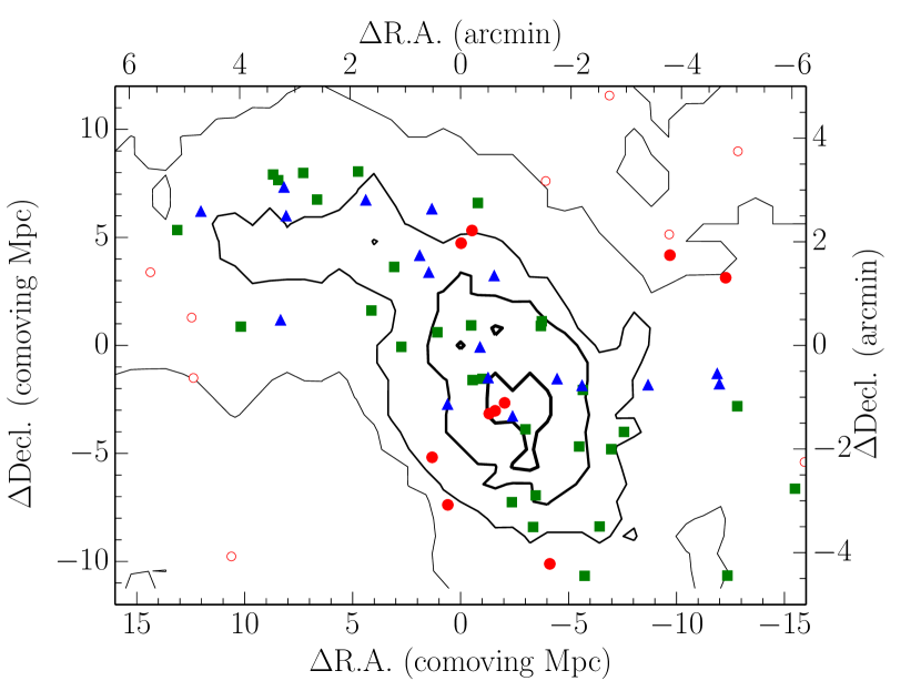
Figure 1.— Sky distribution of the $i^{\prime}$-dropout galaxies and number density contours. Spectroscopically observed galaxies are marked by filled symbols (red circles: protocluster galaxies, blue triangles: field galaxies, green squares: Ly$\alpha$ undetected objects), and spectroscopically unobserved galaxies are shown by open circles. The origin (0,0) is $(\mathrm{R.A.},\mathrm{Decl.})=(13:24:29.0,+27:17:19.1)$, which is defined as the center of the figure. The lines show the number density contours of $i^{\prime}$-dropout galaxies from $6\sigma$ to $0\sigma$ with a step of $2\sigma$. The local number density was estimated by counting $i^{\prime}$-dropout galaxies within a fixed aperture of $2\farcm 1$ radius ($5\,\mathrm{Mpc}$). $\sigma$ is the standard deviation of the local number densities. It can be clearly seen that all $i^{\prime}$-dropout galaxies in/around the overdense region were spectroscopically observed.

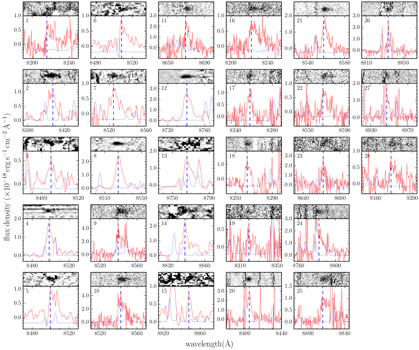
Figure 2.— Spectra of 28 galaxies having a Ly$\alpha$ emission line. The vertical dashed lines indicate the peak of the Ly$\alpha$ emission line. The blue solid lines represent the sky lines. The object IDs are indicated at the upper left corner (Column 1 of Table 1).

2.2. Complete Follow-up Spectroscopy of the Protocluster

We used the DEIMOS on the Keck II telescope in Multi-Object Spectroscopy (MOS) mode (Faber et al., 2003). The DEIMOS observation was conducted using a $830\,\mathrm{line\,mm^{-1}}$ grating and the OG550 order blocking filter, providing a wavelength coverage of $7000\,\mathrm{\AA}-10000\,\mathrm{\AA}$ with a pixel resolution of $0.47\,\mathrm{\AA\,pix^{-1}}$. The slit width was set to $1\farcs 0$, giving a spectral resolution of $4.3\,\mathrm{\AA}$ ($R\sim 2000$). We targeted 34 $i^{\prime}$-dropout galaxies in/around the protocluster; 14 of these were already observed by our previous follow-up spectroscopy but no signal was detected. In addition, we allocated slits to eleven secondary targets having $i^{\prime}-z^{\prime}>1.0$. The observation was carried out on April 8, 2013, and the sky condition was good with a seeing of $\sim 0\farcs 6$. We obtained 15 exposures for a total integration time of 7.5 hours. Long slit exposures of a standard star, BD$+$332642, were used for the flux calibration. The data were reduced using the pipeline spec2d. Furthermore, we obtained spectra of two $i^{\prime}$-dropout galaxies through other MOS observations with Keck/DEIMOS on different projects (Kashikawa et al., 2011).

Combining our previous follow-up spectroscopic observations, we observed 53 $i^{\prime}$-dropout galaxies in/around the protocluster region. The DEIMOS pointing of this observation was set to cover both the protocluster region and a $2\sigma$ overdense region extending from the main protocluster region. The sky distribution of $i^{\prime}$-dropout galaxies and spectroscopically observed galaxies are shown in Figure 1. All of the $i^{\prime}$-dropout galaxies in the $2\sigma$ significant overdense region were completely observed with spectroscopy.

Table 1Observed Properties of the 28 Spectroscopic Confirmed Galaxies

ID	R.A.	Decl.	$z^{\prime}$	$i^{\prime}-z^{\prime}$	$z$	$M_{\mathrm{UV}}$	$f_{\mathrm{Ly\alpha}}$	$L_{\mathrm{Ly\alpha}}$	$EW_{\mathrm{rest}}$	$S_{w}$
	(J2000)	(J2000)	(mag)	(mag)		(mag)	($10^{-18}\,\mathrm{erg\,s^{-1}\,cm^{-2}}$)	($10^{42}\,\mathrm{erg\,s^{-1}}$)	(Å)	(Å)
1	13:24:31.8	+27:18:44.2	$25.91\pm 0.04$	1.48	$5.758^{+0.001}_{-0.001}$	$-20.74\pm 0.04$	$4.39\pm 0.86$	$1.59\pm 0.31$	$7.7\pm 1.4$	$5.61\pm 1.36$
2	13:24:18.4	+27:16:32.6	$25.69\pm 0.03$	1.70	$5.916^{+0.002}_{-0.002}$	$-20.97\pm 0.03$	$12.49\pm 0.36$	$4.82\pm 0.14$	$19.0\pm 0.8$	$5.66\pm 1.14$
3	13:24:25.2	+27:16:12.2	$27.02\pm 0.09$	1.89	$5.984^{+0.006}_{-0.002}$	$-19.60\pm 0.10$	$4.95\pm 0.51$	$1.96\pm 0.20$	$29.6\pm 4.1$	$3.41\pm 4.03$
4	13:24:30.2	+27:14:13.5	$26.81\pm 0.08$	1.96	$5.991^{+0.002}_{-0.002}$	$-19.51\pm 0.11$	$15.42\pm 0.63$	$6.12\pm 0.25$	$107.5\pm 12.2$	$5.26\pm 1.21$
5	13:24:26.0	+27:16:03.0	$26.50\pm 0.06$	1.71	$5.992^{+0.002}_{-0.002}$	$-20.11\pm 0.10$	$8.16\pm 0.58$	$3.24\pm 0.23$	$31.4\pm 3.8$	$10.01\pm 0.93$
6	13:24:21.3	+27:13:04.8	$25.91\pm 0.04$	2.65	$5.999^{+0.002}_{-0.006}$	$-20.79\pm 0.04$	$7.59\pm 0.68$	$3.02\pm 0.27$	$15.3\pm 1.5$	$12.28\pm 1.84$
7	13:24:29.0	+27:19:18.0	$26.50\pm 0.06$	1.60	$6.012^{+0.002}_{-0.002}$	$-20.11\pm 0.07$	$7.87\pm 1.50$	$3.15\pm 0.60$	$30.7\pm 6.2$	$5.06\pm 1.84$
8	13:24:28.1	+27:19:32.8	$26.10\pm 0.04$	1.54	$6.012^{+0.002}_{-0.002}$	$-20.32\pm 0.06$	$21.34\pm 0.57$	$8.54\pm 0.23$	$70.8\pm 4.5$	$4.07\pm 0.73$
9	13:24:26.5	+27:15:59.7	$25.47\pm 0.03$	1.91	$6.025^{+0.003}_{-0.004}$	$-21.03\pm 0.05$	$29.94\pm 2.63$	$12.04\pm 1.06$	$50.9\pm 5.1$	$8.00\pm 0.21$
10	13:24:31.5	+27:15:08.8	$25.91\pm 0.06$	1.95	$6.027^{+0.002}_{-0.002}$	$-20.43\pm 0.10$	$27.36\pm 2.95$	$11.02\pm 1.19$	$95.7\pm 14.2$	$8.12\pm 0.23$
11	13:24:26.1	+27:18:40.5	$26.59\pm 0.06$	2.32	$6.131^{+0.003}_{-0.003}$	$-19.87\pm 0.11$	$12.38\pm 1.19$	$5.19\pm 0.50$	$67.0\pm 9.5$	$4.24\pm 0.35$
12	13:24:31.6	+27:19:58.2	$26.47\pm 0.06$	2.07	$6.190^{+0.002}_{-0.002}$	$-19.36\pm 0.19$	$24.48\pm 0.69$	$10.49\pm 0.29$	$213.1\pm 40.3$	$4.69\pm 0.88$
13	13:24:44.3	+27:19:50.0	$26.43\pm 0.06$	2.49	$6.211^{+0.004}_{-0.007}$	$-20.23\pm 0.09$	$15.01\pm 0.74$	$6.48\pm 0.32$	$58.7\pm 6.1$	$7.24\pm 1.24$
14	13:24:20.6	+27:16:40.5	$27.01\pm 0.09$	1.90	$6.271^{+0.002}_{-0.005}$	$-19.35\pm 0.22$	$14.28\pm 0.94$	$6.30\pm 0.42$	$136.4\pm 32.1$	$6.25\pm 0.62$
15	13:24:32.6	+27:19:04.0	$25.54\pm 0.03$	1.47	$6.278^{+0.005}_{-0.002}$	$-21.75\pm 0.03$	$4.00\pm 0.50$	$1.77\pm 0.22$	$2.2\pm 0.3$	$2.35\pm 3.20$
16	13:24:44.8	+27:17:48.8	$26.10\pm 0.04$	1.76	$5.764^{+0.001}_{-0.001}$	$-20.55\pm 0.04$	$7.08\pm 0.72$	$2.57\pm 0.26$	$16.0\pm 1.8$	$6.82\pm 0.71$
17	13:24:44.5	+27:20:23.4	$26.70\pm 0.07$	1.09	$5.791^{+0.001}_{-0.001}$	$-19.95\pm 0.07$	$6.18\pm 0.71$	$2.27\pm 0.26$	$26.6\pm 3.3$	$2.80\pm 1.39$
18	13:24:27.4	+27:17:17.4	$26.62\pm 0.06$	1.75	$5.797^{+0.001}_{-0.001}$	$-20.03\pm 0.06$	$5.67\pm 0.70$	$2.09\pm 0.26$	$23.3\pm 2.9$	$2.15\pm 0.42$
19	13:24:26.6	+27:16:41.7	$26.84\pm 0.08$	1.74	$5.844^{+0.001}_{-0.001}$	$-19.84\pm 0.08$	$1.26\pm 0.33$	$0.47\pm 0.12$	$6.3\pm 1.5$	$-0.66\pm 0.67$
20	13:24:12.7	+27:16:33.3	$25.99\pm 0.04$	1.39	$5.914^{+0.001}_{-0.001}$	$-20.67\pm 0.04$	$13.17\pm 0.74$	$5.08\pm 0.29$	$30.2\pm 2.2$	$2.51\pm 0.27$
21	13:24:10.8	+27:19:04.0	$26.61\pm 0.06$	2.30	$6.039^{+0.001}_{-0.001}$	$-19.88\pm 0.09$	$10.95\pm 0.99$	$4.43\pm 0.40$	$54.6\pm 8.3$	$6.04\pm 0.57$
22	13:24:05.9	+27:18:37.7	$26.87\pm 0.08$	2.04	$6.047^{+0.001}_{-0.001}$	$-19.84\pm 0.09$	$3.97\pm 0.72$	$1.61\pm 0.29$	$20.9\pm 4.5$	$4.53\pm 0.82$
23	13:24:30.2	+27:16:10.8	$26.15\pm 0.05$	2.21	$6.125^{+0.001}_{-0.001}$	$-20.61\pm 0.06$	$9.37\pm 0.60$	$3.92\pm 0.25$	$28.4\pm 2.4$	$0.93\pm 0.19$
24	13:24:37.3	+27:20:08.5	$26.00\pm 0.04$	2.88	$6.224^{+0.001}_{-0.001}$	$-20.93\pm 0.06$	$13.46\pm 1.37$	$5.85\pm 0.59$	$26.9\pm 3.9$	$30.20\pm 6.33$
25	13:24:51.7	+27:19:55.3	$26.84\pm 0.08$	2.07	$6.252^{+0.001}_{-0.001}$	$-19.99\pm 0.12$	$8.90\pm 0.57$	$3.90\pm 0.25$	$43.1\pm 6.6$	$0.87\pm 0.90$
26	13:24:06.6	+27:16:46.4	$26.81\pm 0.08$	1.79	$6.267^{+0.001}_{-0.001}$	$-20.28\pm 0.09$	$4.99\pm 0.40$	$2.20\pm 0.18$	$19.3\pm 2.5$	$2.00\pm 0.11$
27	13:24:24.5	+27:15:56.9	$26.69\pm 0.07$	2.22	$6.359^{+0.001}_{-0.001}$	$-20.25\pm 0.12$	$14.07\pm 0.71$	$6.41\pm 0.32$	$58.1\pm 8.4$	$8.28\pm 2.03$
28	13:24:06.5	+27:16:34.3	$26.97\pm 0.09$	1.94	$6.549^{+0.001}_{-0.001}$	$-20.92\pm 0.10$	$4.39\pm 0.64$	$2.14\pm 0.31$	$9.3\pm 2.0$	$3.86\pm 1.35$

3. RESULTS

From the observation as shown in above section, 14 emission lines are identified by careful examination of two- and one-dimensional spectra. All emission lines in our wavelength coverage are single emission lines; thus, there is almost no chance that H$\beta$ or [O III] emission lines contaminate our spectra because the wavelength coverage of our observation is wide enough to detect all these lines simultaneously. However, only [O III]$\lambda 5007$ emission, which is typically the strongest emission among them, may be detected if the other emissions are too faint to detect. We investigated the possibility that H$\alpha$, [O II], and [O III]$\lambda 5007$ emission lines might have contaminated our sample, based on both imaging and spectroscopic data. Haines et al. (2008) demonstrated that $\sim 30\%$ of red-sequence galaxies in the field have ongoing star-formation activity with $\mathrm{EW(H\alpha)}>2\,\mathrm{\AA}$, but they also found that these galaxies disappear at an absolute $r$-band magnitude of $M_{r}\gtrsim-18$. Our samples are much fainter ($>3\,\mathrm{mag}$) than this magnitude, if they were at $z\sim 0.3$ based on the photometry of our samples. Regarding [O II] doublet emission lines, it is possible to distinguish between Ly$\alpha$ and [O II] emission lines based on the line profile. The spectral resolution of our spectroscopic observation is high enough to resolve [O II] emission lines as doublets ($\Delta\lambda=6.3\,\mathrm{\AA}$ at $z\sim 1.3$), although it would be practically difficult to resolve these in most cases due to low signal-to-noise ratio (S/N). In this case, the [O II] emission line should be skewed to blueward, while Ly$\alpha$ emission lines from high redshift galaxies should be skewed to redward. We also calculated weighted skewness, $S_{w}$, which is a good indicator of the line asymmetry (Kashikawa et al., 2006). The asymmetric emission lines with $S_{w}>3$ are evidence of Ly$\alpha$ emission from high redshift galaxies. Although some emission lines of this study have $S_{w}<3$, strong sky lines and low S/N data prevent the accurate determination of skewness in these cases. The red optical color of $i^{\prime}-z^{\prime}>1.5$ may indicate passive or dustier galaxies if they are at $z\sim 1.5$ or 0.7, while [O II] and [O III]$\lambda 5007$ emissions contradict with the prominent emission lines as the sign of high star-formation activity. Furthermore, according to Ly et al. (2007, 2012), [O II] emitters at $z\sim 1.5$ and [O III] emitters at $z\sim 0.7$ typically have $i^{\prime}-z^{\prime}\sim 0.2$, and almost all have $i^{\prime}-z^{\prime}<1.0$, much bluer than the selection criterion of our sample ($i^{\prime}-z^{\prime}>1.5$). Therefore, it is unlikely that H$\alpha$, [O II], and [O III]$\lambda$5007 emission lines contaminate our sample, and Ly$\alpha$ is the most plausible interpretation for these single emission lines. We can conclude that all single emission lines detected from our $i^{\prime}$-dropout sample as Ly$\alpha$ emission lines at $z\sim 6$.

Although the detection limit of an emission line depends on the wavelength and line width, the $1\sigma$ detection limit for emission lines is typically $6.3\times 10^{-19}\,\mathrm{erg\,s^{-1}\,cm^{-2}}$ in this observation, which was derived from the sky fluctuations in a typical line width ($\sim 6.3\,\mathrm{\AA}$). The limiting observed-frame equivalent width corresponding to the line detection limit is estimated to be $26.4\,\mathrm{\AA}$ ($5.3\,\mathrm{\AA}$) at $m_{z^{\prime}}=27.0\,\mathrm{mag}$ ($25.0\,\mathrm{mag}$).

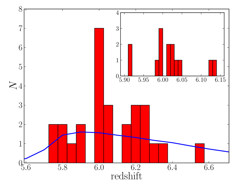
Figure 3.— Redshift distribution of the 28 spectroscopically confirmed galaxies. The bin size is $\Delta z=0.05$. The solid (blue) line shows the selection function of our $i^{\prime}$-dropout selection assuming a uniform distribution normalized to the total number of confirmed emitters. The inset is a close-up of the protocluster redshift range, with a bin size of $\Delta z=0.01$.

One of the targets in this study was already detected as ID1 of Toshikawa et al. (2012), whose S/N was worse in the previous study; thus, the spectroscopic properties of ID1 are replaced with those derived in this study. Therefore, we were able to newly confirm 13 $z\sim 6$ galaxies; thus, in total 28 $z\sim 6$ galaxies, including the 15 in Toshikawa et al. (2012), are identified in/around the overdense region. We estimated the observed properties of the spectroscopically confirmed galaxies, such as UV absolute magnitude ($M_{\mathrm{UV}}$), Ly$\alpha$ luminosity ($L_{\mathrm{Ly\alpha}}$), and rest-frame Ly$\alpha$ equivalent width ($EW_{\mathrm{rest}}$). Although faint continuum flux could not be detected in the observed spectra, $M_{\mathrm{UV}}$ were estimated from the $z^{\prime}$-band magnitudes by subtracting the spectroscopically measured Ly$\alpha$ flux and assuming flat UV continuum spectra ($f_{\nu}=\mathrm{constant}$). The spectra and observed properties of all these galaxies are provided in Figure 2 and Table 1. The redshift distribution is shown in Figure 3. It is clear that ten galaxies are clustered in a narrow redshift range between $z=5.984$ and $z=6.047$ ($\Delta z\lesssim 0.06$), corresponding to the radial distance of $26.1\,\mathrm{Mpc}$ in comoving units. The central redshift of the protocluster is estimated to be $z=6.01$ using biweight (Beers et al., 1990) of ten galaxies. This concentration is about 4.5 times higher than the number expected from a homogeneous distribution in redshift space.

4. COMPARISON WITH MODEL PREDICTIONS

We found a protocluster with $6\sigma$ overdensity at $z=6.01$, but how large is the dark matter halo that it will evolve into at $z=0$? To answer this question, it is necessary to compare our observations with theoretical predictions about the descendants of high redshift overdensities by tracing hierarchical merging histories. Overzier et al. (2009) and Chiang et al. (2013) investigated the relation between galaxy overdensity at high redshift and dark matter halo mass at $z=0$ by using a combination of $N$-body dark matter simulations and semi-analytic galaxy formation models. They systematically studied cluster development from $z\sim 6$ to $z=0$ and found clear correlations between overdensity at high redshift and halo mass at $z=0$, depending on e.g., the sample selection, search volume, and redshift accuracy of the tracer galaxies, as well as the mass of the clusters. Here, we perform a new simulation specifically designed to match the observational details of our $i^{\prime}$-dropout survey as closely as possible. This design is important because our target selection is characterized by a rather broad photometric selection at $z=6\pm 0.5$ compared with the cases described by Chiang et al. (2013). We will connect directly the observed quantity, the significance of the overdensity of the surface number density, to the dark matter halo mass at $z=0$.

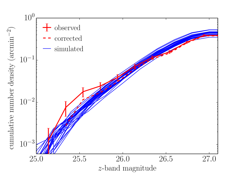
Figure 4.— Number counts of the $i^{\prime}$-dropout galaxies. The red and blue solid lines indicate the observed galaxies in the SDF and those from in the 24 light-cone models, respectively. The number counts of the SDF were corrected for incompleteness. The red dashed line shows the observed number counts corrected for contamination by dwarf stars by using the star count model (Nakajima et al., 2000).

We used the light-cone model constructed by Henriques et al. (2012). A brief outline of the construction of light-cone models is presented below. First, the assembly history of the dark matter halos was traced using an $N$-body simulation (Springel et al., 2005), in which the length of the simulation box was $500\,h^{-1}\,\mathrm{Mpc}$ and the particle mass was $8.6\times 10^{8}\,h^{-1}\,\mathrm{M_{\sun}}$. The distributions of dark matter halos were stored at discrete epochs. Next, the processes of baryonic physics were added to dark matter halos at each epoch using a semi-analytic galaxy formation model (Guo et al., 2011). Based on the intrinsic parameters of galaxies predicted by the semi-analytic model, such as stellar mass, star formation history, metallicity, and dust content, the photometric properties of simulated galaxies were estimated from the stellar population synthesis models developed by Bruzual & Charlot (2003). Then, these simulated galaxies in boxes at different epochs were projected along the line-of-sight, and intergalactic medium (IGM) absorption was applied in order to mimic a pencil-beam survey using the Madau (1995) IGM light-cone set from Overzier et al. (2013). Finally, 24 light-cone models with $1.4\times 1.4\,\mathrm{deg^{2}}$ FoV were extracted using these procedures.

The same color selection applied to the observations (Toshikawa et al., 2012) was also applied to the simulated catalog of each light-cone model. In this analysis, we only used the galaxies whose dark matter halos are composed of more than 100 dark matter particles ($\sim 1\times 10^{11}\,\mathrm{M_{\sun}}$ halo mass), because galaxies’ SEDs in small halos are not stable between redshift snapshots. A color correction was also made to transform the light-cone’s SDSS filter system to Subaru/SprimeCam’s one. We detected $\sim 3000$ $i^{\prime}$-dropout galaxies per $2\,\mathrm{deg^{2}}$ FoV down to the same limiting magnitude of $z^{\prime}$-band, as in the SDF. The number counts of the simulated $i^{\prime}$-dropouts were found to be nearly consistent with those observed in the SDF (Figure 4). Although there is some deviation at the bright end, this is probably caused by the contamination of dwarf stars, which are not included in the model. As in Figure 4, the observed number counts well agree with the simulated ones by correcting for the contamination of dwarf stars, which is estimated by the star count model developed by Nakajima et al. (2000). We also compared the simulated number counts with those of $z\sim 6$ galaxies in Bouwens et al. (2014), applying the selection window for $z\sim 6$ galaxies presented in Bouwens et al. (2014) to light-cone models. Both number counts are almost consistent with each other. Next, we investigated the sky distribution and estimated the local surface number density in the light-cone catalogs in the same way as in the SDF. For each overdense region, the dominant structure was identified as follows. First, we selected the strongest spike in the redshift distribution for that region. Next, we determined the halo ID of the most massive halo in that redshift spike. Finally, the descendant halos at $z=0$ for each overdense region were identified by tracing the halo merger tree of those $z\sim 6$ halos. Figure 5 shows the relation between the significance of the overdensities at $z\sim 6$ and the halo mass at $z=0$. Although there is large scatter, these two quantities are correlated quite closely. The Spearman’s rank correlation coefficient is 0.55, indicating that the probability of no correlation is $<10^{-5}$. We find that 95% (100%) of $>4\sigma$ ($>6\sigma$) overdense regions are expected to include protoclusters. This result suggests that we can detect a real protocluster with high confidence by measuring the overdensity significance if it is more than $4\sigma$ away from the observed surface number density, and also that we can infer its descendant halo mass at $z=0$ based on Figure 5. The protocluster that we found with $6\sigma$ significance at $z\sim 6$ is predicted to evolve into a dark matter halo with a mass of $5\times 10^{14}\,\mathrm{M_{\sun}}$ on average and at least $1\times 10^{14}\,\mathrm{M_{\sun}}$ at $z=0$, suggesting that this is a progenitor of a local galaxy cluster. We also estimated the number density of such overdense regions at $z\sim 6$ based on the large survey volume covered by the simulations. The average number density of regions with $>6\sigma$ significance is $0.42\,\mathrm{deg^{-2}}$ (0.83 per light-cone), though the scatter from field to field is as large as $0.43\,\mathrm{deg^{-2}}$. Considering that our finding was made in a field measuring only $0.24\,\mathrm{deg^{2}}$, this discovery must have been quite serendipitous.

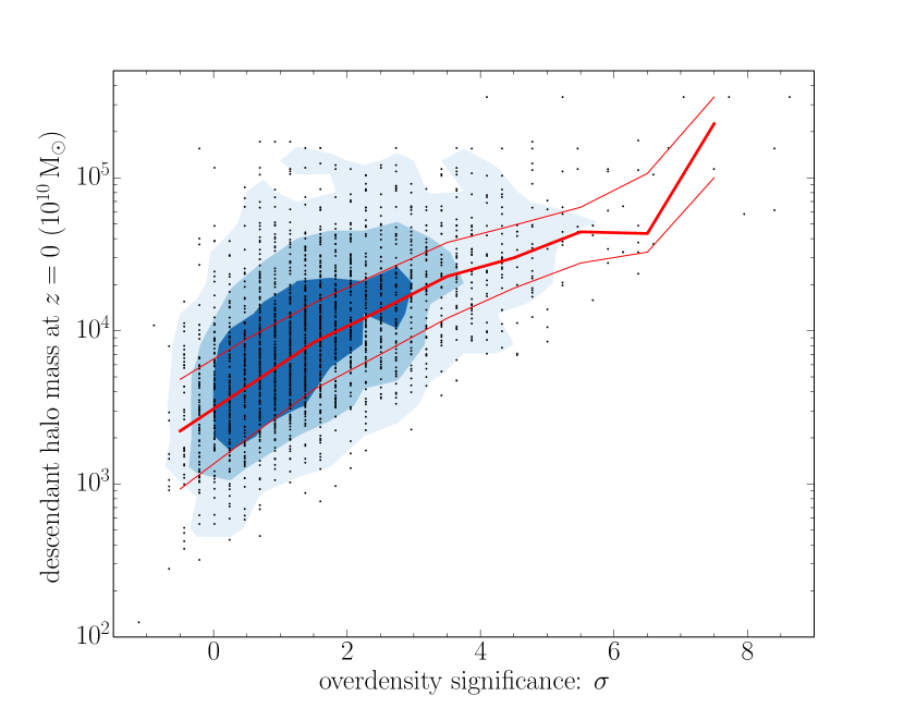
Figure 5.— Relation between surface overdensity at $z\sim 6$ and descendant halo mass at $z=0$. The points represent descendant halo masses in each overdense region. The thick and thin red lines are the median, upper, and lower quartiles. The background contours show the 50, 75, and $95\,\%$ region from dark to light.

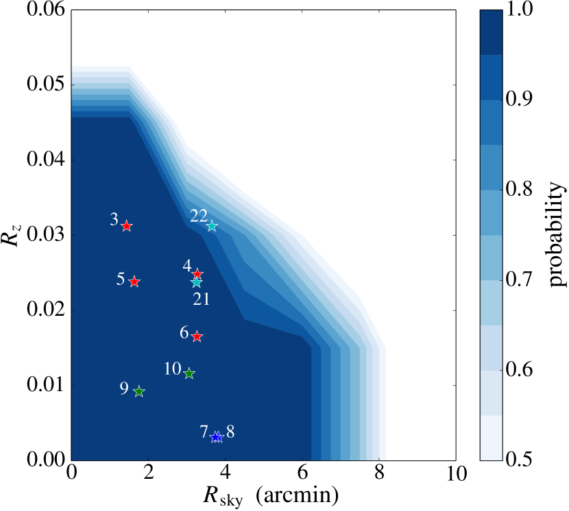
Figure 6.— Probability of merging into a single halo by $z=0$ as a function of distance from the center of the protoclusters at $z\sim 6$. Probability was defined as the fraction of protocluster members among all galaxies at that distance. This probability map was derived from stacking all $>6\sigma$ regions after calculating the probability map of each overdense region. The horizontal and vertical axes indicate spatial and redshift directions, and color contours show the probability. The positions of our ten protocluster members (ID=3-10,21,22) are also plotted using the same color code as that used in Figure 8. The figure shows that is is highly likely that the ten spectroscopically confirmed galaxies will all end up within the same cluster-sized halo at $z=0$.

In addition, we estimated the probability for a galaxy located at a certain position relative to the protocluster center to become a cluster member at $z=0$. Based on the simulation, we can map the galaxy distribution of a protocluster at $z\sim 6$ by tracing back the merger tree of a cluster at $z=0$. Although protoclusters have different structural morphologies, such as filamentary or sheet-like, we estimated the probability by counting the numbers of both descendant cluster members and non-members as a function of the distance to the protocluster center. The center of each protocluster is defined as the peak of the three-dimensional density field, and a spatial map of these probabilities is derived for each protocluster. We extracted 19 $z\sim 6$ protoclusters with $>6\sigma$ overdensity and made a median stack in order to derive a spatial map of the probability that a galaxy will merge into a single halo by $z=0$ as a function of distance from the center of the protocluster (Figure 6). Additionally, we plotted the observed protocluster members within a narrow redshift range (ID=3-10,21,22) measured by our spectroscopy, as shown in Figure 6. The center of the protocluster is simply defined by the middle values between the maximum and the minimum of R.A./Decl./redshift of ten galaxies, which is around $(\Delta\mathrm{R.A.},\Delta\mathrm{Decl.})=(-4,-2)\,\mathrm{Mpc}$ in Figure 1 and $z=6.02$. We found that these ten (nine without ID=22) galaxies will become a single halo by $z=0$ with a probability of $>80\,\%$ ($>95\,\%$). Based on the model prediction, even two galaxies, which are located around $(\Delta\mathrm{R.A.},\Delta\mathrm{Decl.})=(-11,3)\,\mathrm{Mpc}$ in Figure 1, are expected to coalesce into a cluster even though they are located in a region of only $<2\sigma$ significance. This illustrates well that our ten protocluster members are indeed expected to become members of a cluster at $z=0$. It should be noted that the estimate of the center of the observed protocluster involves some uncertainties, because only Ly$\alpha$ emitting galaxies can be identified as protocluster members; detection completeness also grows some uncertainties. In this study, the number of protocluster members is only ten; therefore, we estimated the center of the observed protocluster in various ways, using the average, median, or biweight (Beers et al., 1990) of the ten members’ positions, and checked the differences between these methods. As a result, the uncertainties in the center are $<1.5\,\mathrm{arcmin}$ ($3.6\,\mathrm{Mpc}$) in the spatial and $<0.01$ ($4.2\,\mathrm{Mpc}$) in the redshift direction. Although the most outer galaxy could have a probability of only $50\,\%$ or less in the worst case, most galaxies have a high probability of $>80\,\%$. Therefore, we conclude that these ten galaxies are likely protocluster members.

5. DISCUSSION

Based on comparison with the model prediction in the previous section, we classified 28 spectroscopically confirmed galaxies into two groups: ten protocluster members (ID=3-10,21,22) and 18 non-members (ID=1,2,11-20,23-28). The members are clustered in the redshift range between $z=5.984$ and $z=6.047$ ($\Delta z\lesssim 0.06$), which corresponds to a radial separation of $26.1\,\mathrm{Mpc}$. The properties and distribution of the galaxies within the protocluster are discussed in this section.

5.1. Galaxy Properties

We compared several galaxy properties between members and non-members to investigate whether there was any difference due to their environments at this early epoch. The average and standard deviation of $L_{\mathrm{Ly\alpha}}$, $M_{\mathrm{UV}}$, and $EW_{\mathrm{rest}}$ in the protocluster and field galaxies were estimated, and found that all of these properties of protocluster and field galaxies are consistent with each other within $1\sigma$ scatter, as shown in Table 2. Figure 7 shows that there are no significant differences between the $M_{\mathrm{UV}}$ and Ly$\alpha$ $EW_{\mathrm{rest}}$ distribution between protocluster and field (the p-value derived by the Kolmogorov-Smirnov (KS) test is $>0.3$); however, a possible difference can be seen at the lowest $EW_{\mathrm{rest}}$ bin ($EW_{\mathrm{rest}}<20\,\mathrm{\AA}$). Because both protocluster and field galaxies were observed in the same observing runs, it is unlikely that this difference was caused by a difference in the completeness limit of the spectroscopic observations. Taking into account the completeness limit, the sample in the lowest $EW_{\mathrm{rest}}$ bin mostly consists of the brightest galaxies in $M_{\mathrm{UV}}$. This may imply that the brightest galaxies in the overdense region are older and have more dust, suppressing the Ly$\alpha$ emission compared with those in the field galaxies. Lee et al. (2013) also reported that the median $EW_{\mathrm{rest}}$ of $z=3.78$ protocluster galaxies is higher than that of field galaxies. However, the Ly$\alpha$ emission, which is a resonantly-scattered line, can be affected by many physical parameters such as SFR, dust amount, and geometry of dust and neutral gas (e.g., Shibuya et al., 2014). It is therefore difficult to identify the reason of the possible difference at the lowest $EW_{\mathrm{rest}}$. In this study of a $z=6.01$ protocluster, it should be noted that the difference can be only seen in the lowest $EW_{\mathrm{rest}}$ bin, and there is no significant difference between the $EW_{\mathrm{rest}}$ distribution of the protocluster and the field galaxies as a whole.

Table 2Average of Observed Properties of Protocluster and Field Galaxies

	$L_{\mathrm{Ly\alpha}}$	$M_{\mathrm{UV}}$	$EW_{\mathrm{rest}}$
	($10^{42}\,\mathrm{erg\,s^{-1}}$)	(mag)	(Å)
protocluster	$5.51\pm 3.78$	$-20.16\pm 0.49$	$50.74\pm 31.66$
field	$4.21\pm 2.44$	$-20.34\pm 0.61$	$45.53\pm 52.60$
p-value	0.78	0.78	0.32

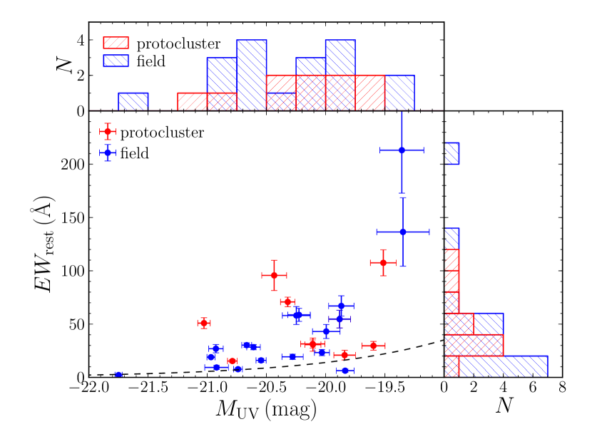
Figure 7.— $EW_{\mathrm{rest}}$ versus $M_{\mathrm{UV}}$ of spectroscopically confirmed galaxies. The histograms in the top and right panels show the $EW_{\mathrm{rest}}$ and $M_{\mathrm{UV}}$ distributions of the protocluster and field galaxies. Red and blue color represent the protocluster and field galaxies, respectively. The dashed line indicates the $5\sigma$ detection limit of the spectroscopic observation.

We measured the Ly$\alpha$ fraction, which is the fraction of Ly$\alpha$ emitting galaxies among our dropout galaxies. This has been widely studied at $4<z<8$ (e.g., Stark et al., 2010; Schenker et al., 2012; Treu et al., 2013), and the fraction steadily increases toward higher redshift, while it gradually decreases beyond $z=6$, possibly as a signature of reionization. However, those measurements were made using only field galaxies. It is important to compare the Ly$\alpha$ fraction between field galaxies and galaxies in overdense regions in order to ascertain whether it has environmental dependence or not. Since it is impossible to distinguish between member and non-member galaxies in the spectroscopically undetected galaxies, we measured the Ly$\alpha$ fraction in the projected overdense region over $8\times 8\,\mathrm{arcmin^{2}}$, including Ly$\alpha$ emitting galaxies, even if they were found in the field behind and in front of the protocluster. We assumed that the Ly$\alpha$ undetected galaxies are all at $z=6.0$, and calculated their $M_{\mathrm{UV}}$. In this estimate, expected IGM absorption at $z=6.0$ in the $z^{\prime}$-band was also corrected for though the correction is as small as $0.08\,\mathrm{mag}$. We here apply the same color selection criterion of $i^{\prime}-z^{\prime}>1.3$ as in Stark et al. (2011). Our spectroscopic completeness still remains high ($>95\%$) in the overdense region because $i^{\prime}$-dropout galaxies with $1.3<i^{\prime}-z^{\prime}<1.5$ were also observed as secondary targets. We compare our result with the bright sample of Stark et al. (2011), which has the same $M_{\mathrm{UV}}$ range as ours. The fraction in the overdense region was found to be $0.0^{+6.4}_{-0.0}\%$ and $20.0\pm 11.0\%$ for $EW_{\mathrm{rest}}>50\,\mathrm{\AA}$ and $>25\,\mathrm{\AA}$, which are almost the same as in the field at $z\sim 6$.

These results show that we do not find any significant differences in the observed properties between protocluster and field galaxies. This would indicate that this protocluster is still in the early phase of cluster formation, before any environmental effect works on galaxy properties. However, the observed properties of protocluster galaxies in this study are very limited. According to other works for lower-redshift protoclusters, differences in galaxy properties between protocluster and field galaxies begin to appear at $z\sim 2-3$: protocluster galaxies are $\sim 2-3$ times more massive than field galaxies at the same redshift (Steidel et al., 2005; Kuiper et al., 2010; Hatch et al., 2011). In this study, the UV and Ly$\alpha$ properties of the protocluster galaxies are almost the same as those of field galaxies. These properties are closely related to star-formation activity. This could imply that galaxy mergers could scarcely happen even in the high-density region at $z\sim 6$ because galaxies basically contain large amounts of gas in their young phase. Under such conditions, galaxy mergers can ignite bursty star formation. Therefore, the stellar-mass difference as seen at $z=2-3$ could emerge in a later cluster formation phase rather than in this early stage; overdense regions would result in a higher rate of galaxy mergers, which could prolong star formation. However, direct stellar mass measurements using deep infrared imaging of the protocluster at $z=6.01$ will be required to investigate this issue further.

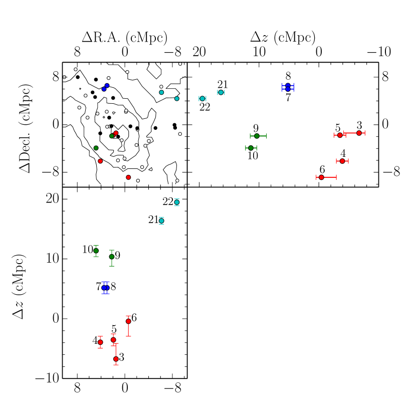
Figure 8.— Three-dimensional distribution of the protocluster galaxies. The points and lines are the $i^{\prime}$-dropout galaxies and number density contours respectively, which are the same as those in Figure 1. The filled points represent the 28 Ly$\alpha$ detected galaxies, and the color-coded points indicate the protocluster galaxies. Possible substructures are grouped by the same color Note that the origin (0,0) of this figure is defined as $(\mathrm{R.A.},\mathrm{Decl.})=(13:24:22.4,+27:16:47.3)$, which is different from that of Figure 1.

5.2. Protocluster Structure

As has been discussed in Toshikawa et al. (2012), the protocluster appears to have some substructure: there are no spectroscopically identified galaxies at the central region of the protocluster, and it is far from virial equilibrium. In this study, the number of spectroscopically identified member galaxies was increased to ten, but their velocity dispersion was found to be still too high ($869\pm 85\,\mathrm{km\,s^{-1}}$) to consider virial equilibrium. Figure 8 presents an updated version of the 3D galaxy distribution in the protocluster after including new spectroscopically identified galaxies; it reveals that the protocluster seems to consist of 4 subgroups of close pairs. Protocluster galaxies having almost the same redshifts happen to be located near to each other in the spatial dimension as well. To discuss this more quantitatively, the histogram of the spatial separation from the nearest galaxy is shown in the left panel of Figure 9. The KS test suggests that the observed histogram is significantly different from a random distribution (the p-value is less than 0.01); random distribution was generated from a uniform distribution in the limited-size box of $17\times 19\times 29\,\mathrm{Mpc^{3}}$, which corresponds to the volume occupied by the ten member galaxies. Furthermore, Figure 9 shows a histogram of the separation from the nearest neighbor of field LAEs. The data were taken from the spectroscopic LAE samples at $z=5.7$ and 6.5 (Kashikawa et al., 2011), which have a high degree of spectroscopic completeness ($\sim 80-90\%$). To compare protocluster and field galaxies more accurately, the difference in average number density between protocluster and field are corrected. The separation of field LAEs is multiplied by $(n_{\mathrm{field}}/n_{\mathrm{protocluster}})^{1/3}\sim 0.6$, where $n_{\mathrm{protocluster}}$ and $n_{\mathrm{field}}$ are the average number density of the protocluster and field, respectively. The p-value of a KS-test between the distribution of field LAEs and that of the protocluster was found to be less than 0.03, suggesting that the excess of close pairs cannot be attributed to the clustering nature of Ly$\alpha$ emitters alone.

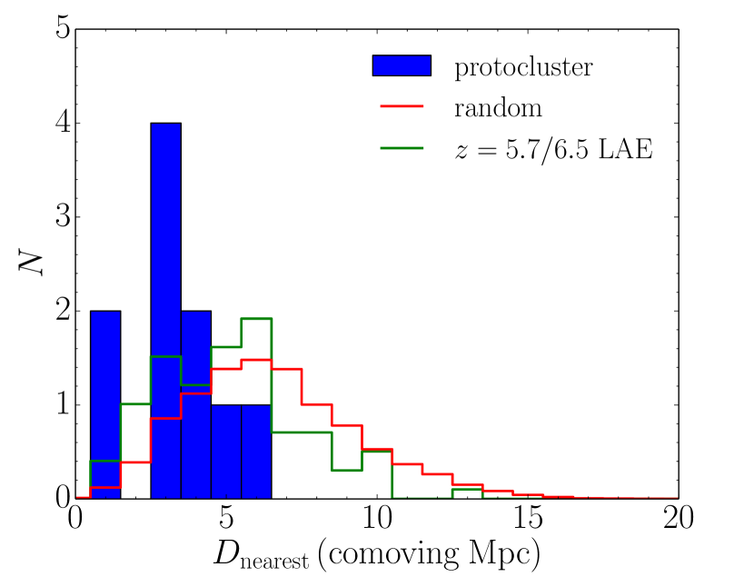
Figure 9.— Distribution of the separation from the first (left) and second (right) nearest galaxy in the protocluster (blue histogram). The red line shows an expected distribution assuming that ten galaxies are randomly distributed in the protocluster region of $17\times 19\times 29\,\mathrm{Mpc^{3}}$, which was defined by the smallest box, including ten protocluster galaxies. This random realization was repeated 1,000 times. The green line shows the distribution of $z=5.7$ and 6.5 LAEs in the SDF (Kashikawa et al., 2011). Separation of field LAEs is corrected for the difference in the average number density between the protocluster and field by multiplying $(n_{\mathrm{field}}/n_{\mathrm{protocluster}})^{1/3}\sim 0.6$.

We also evaluated the separations from the second nearest galaxies (the right panel of Figure 9) based on the same procedure as for the first nearest neighbors. Its separation distribution was found to be reproduced by the random distribution with the p-value of 0.23. Moreover, the separations from $N$th nearest galaxies were also calculated, and shown in Figure 10. The separation, $D$, was fitted as a function of the $N$th ($N>2$) nearest galaxy: $\log(D)=a\times\log(N)+b$ ($a$ and $b$ are free parameters). The values of $a$ and $b$ were $a=0.53\pm 0.04$ and $b=1.82\pm 0.07$ (blue dashed line in Figure 10). The separation was found to be well approximated by this formula for $N>2$, while the observed separation from the first nearest galaxies was found to be smaller with $1.8\sigma$ significance than the extrapolation from the formula. Even if we exclude two galaxies that have exceptionally small separations from the first nearest galaxy, the trend was confirmed with $1.8\sigma$ significance. Actually, as seen in Figure 10, all individual separations from the first nearest galaxy are smaller than the best fitted line. It is a statistically reliable result that galaxy separation from the first nearest galaxy is significantly smaller in this protocluster. Therefore, the protocluster galaxies tend to make galaxy pairs rather than triplets or larger structures. However, the typical separation length ($>100\,\mathrm{kpc}$ in physical units) is too large for galaxy mergers or interactions. This is consistent with Cooke et al. (2010) who found that the fraction of Ly$\alpha$ emission in LBGs is larger in pairs with separation of only $\leqslant 70\,\mathrm{kpc}$ in physical units. We could not find any strong correlation between the separation length and observed properties ($M_{\mathrm{UV}}$, $L_{\mathrm{Ly\alpha}}$, and $EW_{\mathrm{rest}}$).

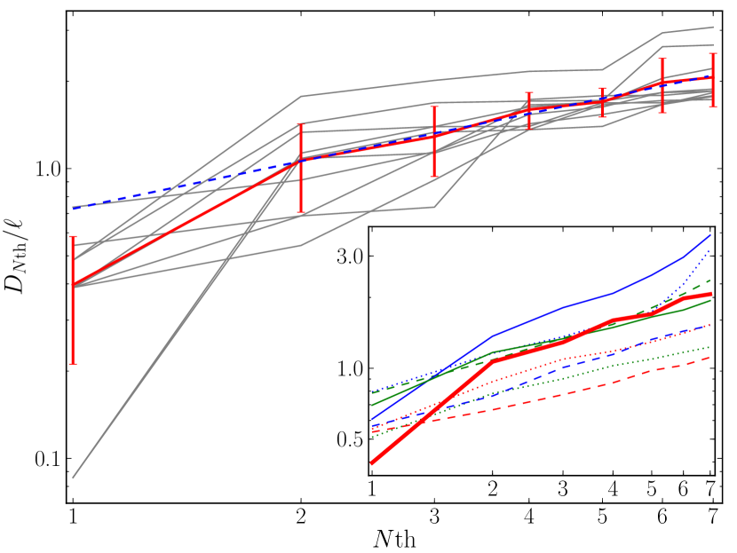
Figure 10.— Galaxy separation from the first to seventh nearest galaxies. In the vertical axis, the galaxy separation is normalized by $\ell$ ($=n^{-1/3}$, where $n$ is the number density). The red and gray lines represent the average and individual separations. The blue dashed line is the best fitted line to the separation from the second to seventh nearest galaxies. The inset shows the same relations in the case of protoclusters at lower redshifts. The solid lines shows the case for LBGs (red: SDF at $z=6.0$ (this study), green: SSA22 at $z=3.1$ (Steidel et al., 1998), blue: MRC 0316-257 at $z=3.1$ (Kuiper et al., 2012)). The dashed and dotted lines show the case for LAEs (dashed red: TN J1338-1942 at $z=4.1$, dashed green: TN J2009-3040 at $z=3.2$ (Venemans et al., 2007), dashed blue: MRC 0316-257 at $z=3.1$ (Venemans et al., 2005), dotted red: MRC 0943-242 at $z=2.9$, dotted green: MRC 0052-241 at $z=2.9$ (Venemans et al., 2007), dotted blue: MRC 1138-262 at $z=2.2$ (Pentericci et al., 2000)).

The inset in Figure 10 shows the same relations in the case of protoclusters at lower redshifts taken from the literature (Steidel et al., 1998; Venemans et al., 2007; Kuiper et al., 2012). Most of the protoclusters, whose members have been identified by Ly$\alpha$ emission, show the smooth relation without a bend at the first nearest neighbor. Interestingly, the protoclusters, SSA22 and MRC 0316-257, whose members are selected by the dropout technique, show a similar trend as our study: smaller separations from the first nearest galaxies than those from the second or higher nearest galaxies. Generally, LBGs have brighter UV luminosity than LAEs; thus, this trend would imply that bright galaxies are located at the core of a protocluster and make pair-like structures, while faint galaxies are more widely distributed. Bright galaxies, presumably more massive, would form structures faster than less massive galaxies. However, this comparison requires many caveats because the limiting magnitudes and spectroscopic completeness are different; in most lower-redshift protoclusters, only $40-60\,\%$ galaxies are spectroscopically observed. We only selected LBGs or LAEs in the above analysis, but various galaxy populations were found in $z\sim 2-3$ protoclusters. For example, Kuiper et al. (2011, 2012) found large subgroups in protoclusters at $z\sim 2-3$, which contain H$\alpha$ and [O III] emitters as well. These results would be consistent with the hierarchical structure formation model: at first, galaxies form small groups like galaxy pairs, and these small groups grow to larger structures through mergers. The cosmic epoch of $z\sim 6$ may be the onset of cluster formation.

5.3. Ancestors of Large-Scale Structure

An interesting distribution of galaxies can be found behind the protocluster region. Four galaxies at $z\sim 6.2$ (color coded by light green in Figure 11) seem to align in the east-west direction at $\Delta\mathrm{Decl.}\sim 6\,\mathrm{Mpc}$, like a filamentary structure, along the $2\sigma$ overdense region. This filamentary structure, which is $80\,\mathrm{Mpc}$ away from the protocluster, is unlikely to merge with the protocluster by $z=0$. However, it is possible that these four galaxies may become another galaxy group by $z=0$ because they span only $<6\,\mathrm{arcmin}$ and $\Delta z<0.06$. It should be noted that the length of large-scale filaments, as seen in the local universe, can reach more than $100\,\mathrm{Mpc}$ (e.g., Park et al., 2012; Smargon et al., 2012; Alpaslan et al., 2014). These galaxies would thus be part of the large-scale structure around a cluster at $z=0$. Therefore, the protocluster at $z=6.01$ might be embedded in a large-scale overdense region. Einasto et al. (2014) found that galaxy properties depend on the global environment like a supercluster, as well as the local environment like a galaxy group. Thus, it will be interesting to carry out further follow-up observations with infrared imaging on this protocluster region in order to investigate galaxy properties in various environments, such as protoclusters, filaments, and fields.

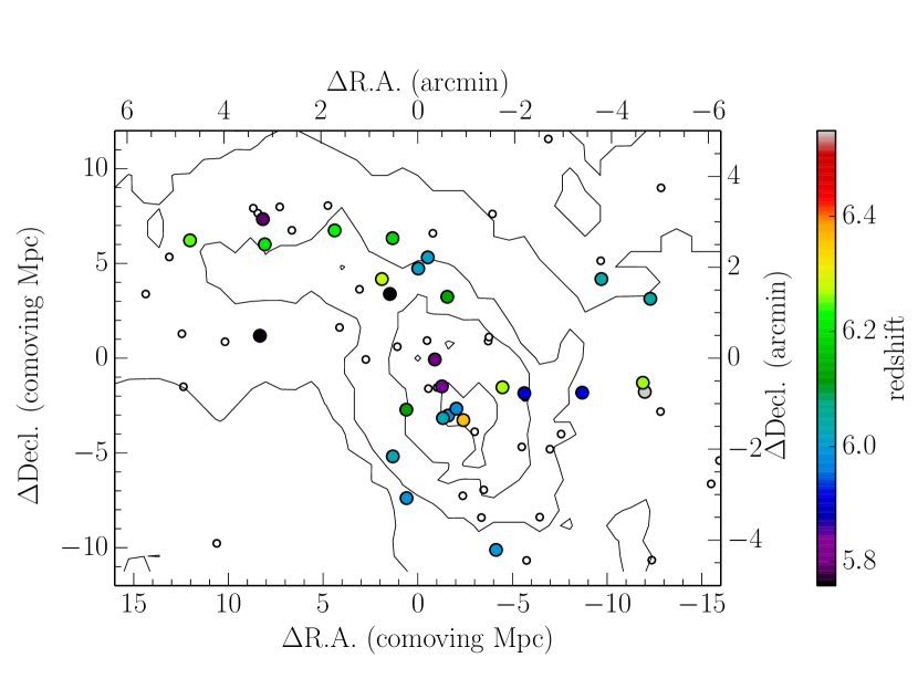
Figure 11.— Sky distribution of the Ly$\alpha$ detected galaxies (filled circles) and the $i^{\prime}$-dropout galaxies (open circles). The redshifts of the Ly$\alpha$ detected galaxies are shown by the color code indicated in the legend at the right. The origin is the same as that of Figure 1. The redshift of the protocluster corresponds to the light blue, and $z\sim 6.2$ galaxies (light green) appear to align in the east-west direction at $\Delta\mathrm{Decl.}\sim 6\,\mathrm{Mpc}$, (see the text in the discussion §5.3).

6. CONCLUSIONS

In this study, we have presented a systematic spectroscopic observation of the highest redshift protocluster known to date. We performed spectroscopy for all 53 $i^{\prime}$-dropout galaxies down to $27.09\,\mathrm{mag}$ in $z^{\prime}$-band in/around the protocluster region, and Ly$\alpha$ emission of $EW_{\mathrm{rest}}\gtrsim 11\,\mathrm{\AA}$ should be completely detected with $\mathrm{S/N}>3$ in our spectroscopy. The results and implications of this study are summarized below.

1. From this observation, 13 galaxies were newly identified as real $z\sim 6$ galaxies by detecting their Ly$\alpha$ emission lines. Combined with the sample from Toshikawa et al. (2012), 28 galaxies were confirmed to be located at $z\sim 6$. Ten of these are clustered in a narrow redshift range between $z=5.984$ and $z=6.047$ ($\Delta z\lesssim 0.06$), corresponding to a radial separation of $26.1\,\mathrm{Mpc}$.

2. We compared our results with the light-cone models, in which we applied the same $i^{\prime}$-dropout selection and the same overdensity measurements as in the observation. We obtained a relation between the observed overdensity significance at $z\sim 6$ and the predicted dark matter halo mass at $z=0$. Based on this relation, the observed protocluster with $6\sigma$ significance is predicted to grow into a galaxy cluster ($\sim 5\times 10^{14}\,\mathrm{M_{\sun}}$) at $z=0$.

3. We also derive the spatial map of probability for a galaxy located at a certain position relative to the protocluster center to become a cluster member at $z=0$. Based on the map, the ten galaxies within $10\,\mathrm{Mpc}$ from the center of the protocluster are found, with more than an 80% probability, to merge into a single dark matter halo by $z=0$. This clustering of galaxies is consistent with the progenitor of a galaxy cluster.

4. No significant difference in observed galaxy properties, such as $M_{\mathrm{UV}}$, $L_{\mathrm{Ly\alpha}}$, and $EW_{\mathrm{rest}}$, between the protocluster and the field are found except for the brightest galaxies. This suggests that this protocluster is still in the early phase of cluster formation before the onset of any obvious environmental effects. Further multi-wavelength imaging to trace their SEDs from the rest-frame optical to far-infrared wavelength will provide us with clues about possible differences in stellar mass, dust, and gas mass.

5. The velocity dispersion of this protocluster is too high ($869\pm 85\,\mathrm{km\,s^{-1}}$) to consider virial equilibrium. This high velocity dispersion would be caused by the internal three-dimensional structure of the protocluster. We also obtained a statistically reliable result that galaxies tend to form close pairs in the protocluster. These pair-like subgroups will coalesce into a single halo and grow into more massive structures through accretion of material from their surroundings. Filamentary structure was found to be $80\,\mathrm{Mpc}$ away from the protocluster. Although it is not expected to merge with the protocluster, this could become a large-scale structure around the galaxy cluster, as seen in the local universe.

As we have shown, the results obtained in this study are qualitatively and, in many ways, also quantitatively, consistent with the hierarchical structure formation model. The epoch of $z\sim 6$ may be the time when galaxies start to coalesce in order to form a cluster as seen in the local universe. It is necessary to increase the number of observations of protoclusters at $z\sim 6$ and even at lower redshifts to obtain statistical samples of protoclusters across cosmic time, in order to clarify the general features of cluster formation and galaxy evolution in dense regions. Using the new instrument Hyper SuprimeCam (HSC) on the Subaru telescope, we are carrying out an unprecedentedly wide and deep survey over the next five years. Based on the number density estimate of protoclusters in Section 4, $>10$ $z\sim 6$, $>500$ $z\sim 5-4$ protoclusters, and even one $z\sim 7$ protocluster would be discovered from this Subaru strategic survey. These will enable us to derive a more complete picture of cluster formation and galaxy evolution in high density environments.

References

- Alpaslan et al. (2014) Alpaslan, M., et al. 2014, MNRAS, 438, 177
- Beers et al. (1990) Beers, T. C., et al. 1990, AJ, 100, 32
- Benson et al. (2001) Benson, A. J., et al. 2001, MNRAS, 327, 1041
- Bouwens et al. (2012) Bouwens, R. J., 2012, ApJ, 754, 83
- Bouwens et al. (2014) Bouwens, R. J., 2014, arXiv:1403.4295
- Bruzual & Charlot (2003) Bruzual G., & Charlot, S. 2003, MNRAS, 344, 1000
- Butcher & Oemler (1984) Butcher, H., & Oemler, A. 1984, ApJ, 285, 426
- Capak et al. (2011) Capak, P. L., et al. 2011, Nature, 470, 233
- Chiang et al. (2013) Chiang, Y.-K., et al. 2013, ApJ, 779, 127
- Cooke et al. (2010) Cooke, J., et al. 2010, MNRAS, 403, 1020
- De Lucia et al. (2006) De Lucia, G., et al. 2006, MNRAS, 366, 499
- Digby-North et al. (2010) Digby-North, J. A., et al. 2010, MNRAS, 407, 846
- Dressler (1980) Dressler, A. 1980, ApJ, 236, 351
- Einasto et al. (2014) Einasto, M., et al. 2014, A&A, 562, A87
- Faber et al. (2003) Faber, S.M., et al. 2003, Proc. SPIE, 4841, 1657
- Guo et al. (2011) Guo, Q., et al. 2011, MNRAS, 413, 101
- Haines et al. (2008) Haines, C. P., et al. 2008, MNRAS, 385, 1201
- Haines et al. (2009) Haines, C. P., et al. 2009, ApJ, 704, 126
- Hatch et al. (2011) Hatch, N. A., et al. 2011, MNRAS, 415, 2993
- Henriques et al. (2012) Henriques, B. M. B., et al. 2012, MNRAS, 421, 2904
- Kauffmann et al. (1999) Kauffmann, G., et al. 1999, MNRAS, 303, 188
- Kashikawa et al. (2006) Kashikawa, N., et al. 2006, ApJ, 648, 7
- Kashikawa et al. (2011) Kashikawa, N., et al. 2011, ApJ, 734, 119
- Kodama et al. (2007) Kodama, T., et al. 2007, MNRAS, 377, 1717
- Kubo et al. (2013) Kubo, M., et al. 2013, ApJ, 778, 170
- Kuiper et al. (2010) Kuiper, E., et al. 2010, MNRAS, 405, 969
- Kuiper et al. (2011) Kuiper, E., et al. 2011, MNRAS, 415, 2245
- Kuiper et al. (2012) Kuiper, E., et al. 2012, MNRAS, 425, 801
- Lerchster et al. (2011) Lerchster, M., et al. 2011, MNRAS, 411, 2667
- Lee et al. (2013) Lee, K.-S., et al. 2013, ApJ, 771, 25
- Lee et al. (2014) Lee, K.-S., et al. 2014, arXiv:1405.2620
- Lemaux et al. (2014) Lemaux, B. C., et al. 2014, arXiv:1403.4230
- Ly et al. (2007) Ly, C., et al. 2007, ApJ, 657, 738
- Ly et al. (2012) Ly, C., et al. 2012, ApJ, 757, 63
- Madau (1995) Madau, P. 1995, ApJ, 441, 18
- Malhotra et al. (2005) Malhotra, S. et al. 2005, ApJ, 626, 666
- Malkan et al. (1996) Malkan, M. A., et al. 1996, ApJ, 468, L9
- Maraston (2005) Maraston, C. 2005, MNRAS, 362, 799
- Matsuda et al. (2011) Matsuda, Y., et al. 2011, MNRAS, 410, L13
- Mawatari et al. (2012) Mawatari, K., et al. ApJ, 759, 133
- Nakajima et al. (2000) Nakajima, T., et al. 2000, ApJ, 120, 2488
- Popesso et al. (2011) Popesso, P., et al. 2011, A&A, 532, A145
- Rasmussen et al. (2012) Rasmussen, J., et al. 2012, ApJ, 757,122
- Ouchi et al. (2005) Ouchi, M., et al. 2005, ApJ, 620, L1
- Overzier et al. (2009) Overzier, R. A., et al. 2009, ApJ, 704, 548
- Overzier et al. (2013) Overzier, R. A., et al. 2013, MNRAS, 428, 778
- Park et al. (2012) Park, C., et al. 2012, ApJ, 759, L7
- Pentericci et al. (2000) Pentericci, L., et al. 2000, A&A, 361, L25
- Schenker et al. (2012) Schenker, M. A., et al. 2012, ApJ, 744, 179
- Shibuya et al. (2014) Shibuya, T., et al. 2014, arXiv:1402.1168
- Smargon et al. (2012) Smargon, A., et al. 2012, MNRAS, 423, 856
- Springel et al. (2005) Springel, V., et al. 2005, Nature, 435, 629
- Stark et al. (2010) Stark, D., et al. 2010, MNRAS, 408, 1628
- Stark et al. (2011) Stark, D., et al. 2011, ApJ, 728, L2
- Steidel et al. (1998) Steidel, C. C., et al. 1998, ApJ, 492, 428
- Steidel et al. (2005) Steidel, C. C., et al. 2005, ApJ, 626, 44
- Stiavelli et al. (2005) Stiavelli, M., et al. 2005, ApJ, 622, L1
- Tamura et al. (2010) Tamura, Y., et al. 2010, ApJ, 724, 1270
- Thomas et al. (2005) Thomas, D., et al. 2005, ApJ, 621, 673
- Toshikawa et al. (2012) Toshikawa, J., et al. 2012, ApJ, 750, 137
- Trenti et al. (2012) Trenti, M., et al. 2012, ApJ, 746, 55
- Treu et al. (2013) Treu, T., et al. 2013, ApJ, 775, L29
- Venemans et al. (2005) Venemans, B. P., et al. 2005, A&A, 431, 793
- Venemans et al. (2007) Venemans, B. P., et al. 2007, A&A, 461, 823
- Visvanathan & Sandage (1977) Visvanathan, N., & Sandage, A. 1977, ApJ, 216, 214
- von der Linden et al. (2007) von der Linden, A., et al. 2007, MNRAS, 379, 867
- Wilkins et al. (2011) Wilkins, S. M., et al. 2011, MNRAS, 417, 717
- Zheng et al. (2006) Zheng, W. et al. 2006, ApJ, 640, 574
- Zirm et al. (2008) Zirm, A. W., et al. 2008, ApJ, 680, 224