Gravitational collisions and the quark-gluon plasma

Wilke van der Schee,

Abstract

This thesis addresses the thermalisation of heavy-ion collisions within the context of the AdS/CFT duality. The first part clarifies the numerical set-up and studies the relaxation of far-from-equilibrium modes in homogeneous systems. Less trivially we then study colliding shock waves and uncover a transparent regime where the strongly coupled shocks initially pass right through each other. Furthermore, in this regime the later plasma relaxation is insensitive to the longitudinal profile of the shock, implying in particular a universal rapidity shape at strong coupling and high collision energies. Lastly, we study radial expansion in a boost-invariant set-up, allowing us to find good agreement with head-on collisions performed at the LHC accelerator.

As a secondary goal of this thesis, a special effort is made to clearly expose numerical computations by providing commented Mathematica notebooks for most calculations presented. Furthermore, we provide interpolating functions of the geometries computed, which can be of use in other projects.

Promotors: Gleb Arutyunov and Thomas Peitzmann

Publications

This thesis is based on the following publications:

1. Jorge Casalderrey-Solana, Michal Heller, David Mateos and Wilke van der Schee, Longitudinal Coherence in a Holographic Model of Asymmetric Collisions,
   Physical Review Letters 112, 221602 (2014) or arxiv:1312.2956

2. Wilke van der Schee, Paul Romatschke and Scott Pratt,
   A fully dynamical simulation of central nuclear collisions,
   Physical Review Letters 111, 222302 (2013) or arxiv:1307.2539

3. Jorge Casalderrey-Solana, Michal Heller, David Mateos and Wilke van der Schee, From full stopping to transparency in a holographic model of heavy ion collisions, Physical Review Letters 111, 181601 (2013) or arxiv:1305.4919

4. Michal Heller, David Mateos, Wilke van der Schee and Miquel Triana,
   Holographic isotropization linearized, JHEP 09 (2013) 026 or arxiv:1304.5172

5. Wilke van der Schee, Quarks, gluonen en zwarte gaten,
   Nederlands Tijdschrift voor Natuurkunde 79 112-114 (mei 2013)

6. Wilke van der Schee, Holographic thermalization with radial flow,
   Physical Review D 87, 061901 (R) (2013) or arxiv:1211.2218

7. Michal Heller, David Mateos, Wilke van der Schee and Diego Trancanelli,
   Strong coupling isotropization simplified,
   Physical Review Letters 108, 191601 (2012) or arxiv:1202.0981

Chapter 1 Introduction

The theory of quarks and gluons, quantum chromodynamics (QCD), has been well established for decades now. But while the basic Lagrangian of the theory is well known, the non-perturbative nature of this strong force makes it hard to make practical use of the theory, especially in situations that are out-of-equilibrium. In particular, it is still poorly understood how a quark-gluon plasma forms in collisions of relativistic heavy ions, such as performed at the RHIC and LHC accelerators.

In this thesis we try to address this problem using the AdS/CFT duality. Although this duality is only understood for theories related to QCD, it is especially well suited to treat strong coupling and may as such teach us about similar phenomena in QCD. In the future, the hope is to get a better understanding of non-perturbative quantum theories, such as QCD.

1.1 Relativistic heavy ion collisions

Colliding highly relativistic nuclei can create a very dense and hot plasma of quarks and gluons, the so-called quark-gluon plasma. The temperature of this plasma can reach over $10^{12}K$, which is as hot as the universe a millisecond after the big bang. Of course, the scale is very small: a typical collision lasts only $10\,\text{fm}/c$ and takes place within a sphere of radius $15\,\text{fm}$. Nevertheless, at the Large Hadron Collider (LHC) these collisions can create about 26.000 particles, the analysis of which teaches us about conditions shortly after the big bang, and more importantly about QCD in general.

Colliders such as RHIC (Relativistic Heavy Ion Collider) and LHC collide gold nuclei (79 protons and 118 neutrons) or lead nuclei (82 protons and 126 neutrons) respectively. At the highest energy RHIC can achieve, each proton and neutron has an energy of 100 GeV, so they are Lorentz contracted by a factor of one hundred. LHC achieves an even higher energy of 1.38 TeV, giving a Lorentz factor of more than a thousand. In both these colliders the ions move with equal energies in opposite directions in the beam line. At the location of the detectors both beam lines cross, such that some nuclei will hit each other, thereby creating the quark-gluon plasma.

For our purposes we can approximate a nucleus as a smooth distribution of energy, shaped as a Lorentz boosted sphere with radius $R\simeq 6.5\,\text{fm}$. In this simplification, the two colliding nuclei will hit randomly, where the chance $p$ of the distance between both centres $b$ (impact parameter) being less than $r$ is given by

$$p(b<r)=r^{2}/4R^{2}.$$ (1.1.1)

The protons and neutrons of the nucleus which do not hit the other nucleus are called spectators since they have little effect on the collision, as illustrated in 1.1. This means that events with a small impact parameter (lower centrality) will produce many more particles, making a reliable measurement of centrality relatively straightforward.

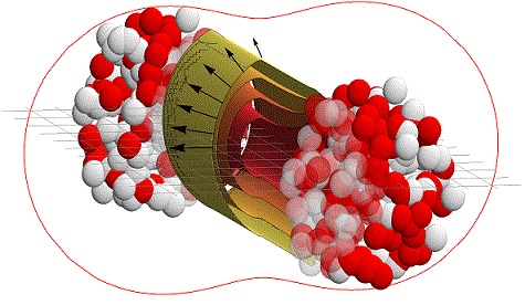
Figure 1.1: A cartoon of a typical heavy-ion collision of impact parameter $b=6\,\text{fm}$. The two Lorentz contracted ions move ultrarelativistically along the z-axis; the nucleons in the non-overlapping are called spectators and just fly on. The nucleons in the collision region (opaque) collide and most of their energy ends up in a quark-gluon plasma. The elliptical shape of this region has larger pressure gradient in the short axis, causing particles to be pushed in this direction, as indicated with the red line (elliptic flow). The succes of this hydrodynamic picture was crucial evidence that the dynamics is strongly coupled.

The interesting challenge is to model such collisions theoretically and predict the spectra of the resulting particles spray (fig. 1.2). Of particular interest is the averaged momentum anisotropy in the transverse plane, usually expanded in spherical harmonics [1]:

$$\frac{d\bar{N}}{d\varphi}=\frac{\bar{N}}{2\pi}\left(1+2\sum_{n=1}^{\infty}\bar{v}_{n}\cos(n(\varphi-\bar{\Psi}_{n}))\right),$$ (1.1.2)

with $\varphi$ the angle in the transverse plane, $\bar{\Psi}_{n}$ defined such that there are no sine terms, $\bar{N}$ the average number of particles of interest per event and $\bar{v}_{n}$ the anisotropic flow coefficients. The most studied is called the elliptic flow coefficient $\bar{v}_{2}$, which is relatively large for non-central collisions due to the approximately ellipsoidal shape of the interaction region, as illustrated in figure 1.1. Crucially, a (hydrodynamic) expansion will convert this elliptical shape in real space into a similar shape in momentum space, which is experimentally accessible and can thus provide important insights in the details of the expansion.

Although it is currently difficult to make definite statements about the first stages of the quark-gluon plasma by analysing the data, there is good reason to be optimistic for significant future improvements. The large number of events measured (many billions) makes a constraining data set, which has a large potential for distinguishing both the initial stage and the subsequent evolution. For this, one should not only look at for instance $\bar{v}_{2}$ averaged over all particles and events, but one can look at $v_{n}$ depending on transverse momentum, rapidity and particle species, or one can look at four and higher order particle correlations, fluctuations from event to event, or even correlations between two different $v_{n}$. Furthermore, one can vary the energy of the colliding nuclei or change the nuclei themselves, thereby changing the collision geometry. At RHIC this has recently been started, which resulted in a large amount of data, which interestingly does not seem to be fully captured by current hydrodynamic models [2].

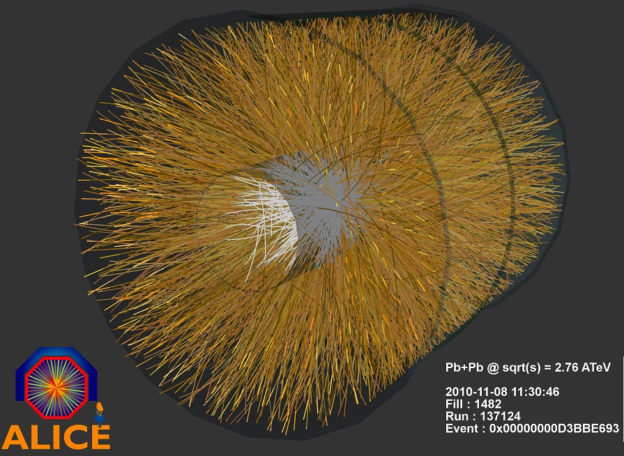
Figure 1.2: A heavy-ion collision, as registered by the ALICE detector. It is a challenge to gain information about the formed quark-gluon plasma from these thousands of tracks, but using correlations and the billions of registered collisions a lot has been learnt. Note that this detector is several meters in size, about $10^{15}$ times bigger than the actual events studied.

One of the main uncertainties in current models of heavy-ion collisions concerns the initial stage directly after the collision, before the quark-gluon plasma is formed. This initial stage is problematic, since it concerns the real-time evolution of many quarks and gluons, which should in principle be described by a fully non-perturbative calculation in QCD. Currently this cannot be achieved, and typically one resorts to weakly coupled calculations, such as used by the colour glass condensate [3, 4]. In this thesis we take a different approach, by using holography, which allows doing a full strongly coupled calculation, albeit not in QCD itself. The hope is that a combination of both weakly and strongly coupled methods will then lead to a better understanding of the initial stage of a heavy-ion collision.

1.2 Holography

The concept of holography goes back to two very old ideas. The first idea is from ’t Hooft, in 1974 [5]. There he noticed, with a very general argument, that strongly coupled $SU(N_{c})$ gauge theories with coupling constant $g$ may simplify when $N_{c}$ is large. When examining Feynman diagrams, a simple counting argument shows that all diagrams of leading order in $N_{c}$, while keeping the ’t Hooft coupling $\lambda=g^{2}N_{c}$ fixed, are planar (they can be drawn on a plane). If one combines this result with the idea that the path integral may be rewritten as a string theory, one sees that this string theory will not contain loops if $N_{c}$ is large, thereby making computations much easier.

A relatively independent argument comes from black hole thermodynamics, where it was noticed early on that the entropy of a black hole scales with the area of the black hole horizon [6]. The implications of this scaling go much beyond the study of just black holes. In a thought experiment one can imagine collapsing any region of spacetime to a black hole, whereby entropy necessarily needs to increase. The only possible conclusion is that any region of spacetime has an entropy bounded by its area [7, 8, 9]. This is of little practical concern, due to the large prefactor, but it naturally leads to the idea that any theory with gravity is fundamentally holographic: it can be described by a theory with one dimension less.

More recently in 1997, Maldacena made both ideas precise in an extraordinary paper [10] (see also [11, 12]). Here he conjectured an exact duality, AdS/CFT, between type IIB string theory on a five dimensional anti-de-Sitter (AdS) background with conformal super-Yang-Mills gauge theory with four supersymmetries, a $SU(N_{c})$ gauge group and living in four dimensions (the CFT: $\mathcal{N}=4$ SYM). So indeed he found a string theory dual of a $SU(N_{c})$ gauge theory, which simplifies to a free string theory when $N_{c}$ is large. Moreover, the string theory reduces to gravity in the classical, non-string, limit and this duality provides the precise holographic dictionary to a non-gravitational theory living in one dimension less [13].

Although the above arguments are very general it has so far only been possible to find a precise dual for specific gauge theories, with usually quite some supersymmetry. In particular, a realistic dual to (large $N_{c}$) QCD is still far away, and the weak coupling in the ultra-violet (UV) of QCD implies that a full solution will require solving the planar string theory, at least in the UV.

On the other hand, the AdS/CFT correspondence can be generalised and allows studying a wide variety of field theories. Importantly, these field theories do not need to be conformal and can for instance have confinement [14] or a running coupling resembling QCD quite closely, such as in improved holographic QCD [15]. The field theory can have (some of) the supersymmetry broken [16]. Including D7-branes in the bulk can include flavoured quarks [17].

1.3 Relativistic hydrodynamics and fluid/gravity

This thesis deals with the collision of heavy ions, particularly with the initial far-from-equilibrium evolution to a quark-gluon plasma describable using relativistic hydrodynamics. One would be tempted to call this transition ‘thermalisation’, but strictly speaking this is not correct, since we consistently find states described by hydrodynamics where pressures in different directions are different. A completely thermalised fluid cell would have equal pressures, which will be achieved much later than the moment hydrodynamics becomes applicable.

Formally, hydrodynamics can be viewed as a gradient expansion around thermal equilibrium. One starts with an exact (boosted) thermal solution with constant energy density and fluid velocity and then promotes these two to a field, both assumed to vary slowly compared to other scales, which gives the following constitutive relations, up to first order in gradients [18]:

$$T_{\mu\nu} = e\,u_{\mu}u_{\nu}+p[e]\Delta_{\mu\nu}+\pi_{\mu\nu},\text{ where,}$$ (1.3.1)

$$\Delta_{\mu\nu} = g_{\mu\nu}+u_{\mu}u_{\nu}\text{ and }$$ (1.3.2)

$$\pi_{\mu\nu} = -\eta[e]\,\sigma_{\mu\nu}+\mathcal{O}(\partial^{2}),\text{ with}$$ (1.3.3)

$$\sigma_{\mu\nu} = \Delta_{\mu\alpha}\Delta_{\nu\beta}(\nabla^{\mu}u^{\nu}+\nabla^{\nu}u^{\mu})-\frac{2}{d-1}\Delta_{\mu\nu}\Delta_{\alpha\beta}\nabla^{\alpha}u^{\beta},$$ (1.3.4)

where $e$ is the local energy density, $p[e]$ is the equation of state, $u_{\mu}$the local fluid velocity, $\pi_{\mu\nu}$ the shear tensor and $\eta$ the shear viscosity, which is the only non-vanishing transport coefficient in first order conformal hydrodynamics. Note that the fluid velocity and energy density are defined as the timelike eigenvector and associated eigenvalue of the stress tensor ($T_{\mu\nu}u^{\nu}=e\,u_{\mu})$ and that $\sigma$ is transverse and traceless: $u^{\mu}\sigma_{\mu\nu}=\sigma_{\,\mu}^{\mu}=0$. Alternatively one can say that the fluid velocity is defined such that when boosting $T_{\mu\nu}$ with velocity $u_{\mu}$ there is no momentum flow, i.e. $T^{\prime}_{0i}=0$, which is called the Landau frame. Having written down the hydrodynamic constitutive relations it will be essential in this thesis to check if 1.3.1 holds for resulting stress tensors. Also, one can use the conservation equation $\nabla^{\mu}T_{\mu\nu}=0$ to evolve an initial energy density and fluid velocity forward in time.

Problematically, relativistic first-order hydrodynamics contains modes propagating faster than light[19], as can be seen by looking at the dispersion relation at high momenta. These modes contain large gradients and are hence outside the regime of the applicability of hydrodynamics. The acausal modes are therefore not a fundamental problem, but they nevertheless cause instabilities when solving the equations numerically. For this purpose second-order hydrodynamics has been extensively studied [20], which is a causal and numerically stable theory for suitable transport coefficients [18]. Interestingly, in all microscopic theories where these transport coefficients could be computed the second-order hydrodynamics is causal, but it is still an open question if this is always true.

In a recent paper [21] it is shown that the hydrodynamic gradient expansion is not necessarily convergent. This is particularly clear in the example of section 2.3, where we can explicitly find degrees of freedom not described by hydrodynamics, the so-called quasi-normal modes. In [21] this was made precise within AdS/CFT by computing the hydrodynamic expansion up to order 240 in derivatives and identifying in the re-summed series the lowest quasi-normal mode.

While the above describes hydrodynamics on itself, the idea of a link between hydrodynamics and gravity dates back to the eighties. First, the membrane paradigm [22] proposed that an outside observer may view the horizon of a black hole as a membrane. This membrane would behave very much like a fluid, with temperature, heat flow, electrical conductivities and so on. Later on this could be made much more precise using AdS/CFT, where a CFT in the hydrodynamic regime can be precisely identified with the corresponding gravitational system.

Importantly, this fluid/gravity correspondence [23, 24] is not a duality between hydrodynamics and gravity, since the gravitational side also contains non-hydrodynamic degrees of freedom. In this thesis we will mostly be interested in this far-from-equilibrium regime, where there is no hydrodynamic description. We will see, however, that relatively quickly hydrodynamics does become applicable, which can in some sense be rephrased as that black hole horizons equilibrate fast.

1.4 Holography and heavy-ion physics

As is now clear it is possible to use AdS/CFT to study strongly coupled theories in the thermodynamic limit, but it can not be used for any gauge theory, in particular not for QCD itself. Nevertheless, AdS/CFT is one of the only tools to study strongly coupled theories, especially in real-time dynamics where the sign problem makes lattice simulations almost impossible.

There are excellent reviews [25, 26, 27, 28] and a recent book [29] on AdS/CFT applied to heavy-ion collisions. These applications typically focus on three topics. The first and oldest application studies the transport coefficients during the hydrodynamic phase, most famously the shear viscosity [30], $\eta=s/4\pi$ with $s$ the entropy density. While it is already a major achievement of AdS/CFT that one can compute the shear viscosity from a microscopic theory, it is also offers a natural explanation in terms of dissipation near a black hole horizon. The latter suggests that this (small) shear viscosity may be far more universal than just $\mathcal{N}=4$ SYM theory, and indeed heavy-ion experiments suggest a value close to the prediction by AdS/CFT [1].

A second topic often studied is jet quenching. At the very first moment of the collision it is possible to form a pair of ultra-energetic quarks, with energies as large as 100 GeV. These quarks then have to pass through (part of) the quark-gluon plasma, whereby they can lose energy. As the energy of the quark jets can be compared between themselves and also with similar results from (simpler) proton-proton collisions the energy loss can be well estimated experimentally. In QCD itself it is hard to study such an energy loss, but at strong coupling several interesting estimates have been made using AdS/CFT around 2006 [31, 32, 33] and also more recently [34, 35, 36]. This may be of special interest as these quarks have energies much above the quark-gluon plasma temperature and can therefore be used to study QCD at higher energies, whereby the coupling constant is weaker.

Lastly, the far-from-equilibrium initial stage of the collision is an excellent example of real-time dynamics and AdS/CFT is the only available tool to study this if the coupling is strong. In this case the formation of a thermal quark-gluon plasma, dual to a black hole in AdS, really corresponds to black hole formation. There has been previous works on this [37, 38, 39, 40], suggesting that this black hole forms ‘as fast as possible’, within a time shorter than a thermal wavelength. This thesis will focus on this avenue and push these earlier studies to more realistic settings, aiming at a comparison with experimental data.

1.5 Outline

In this thesis we try to address the initial stage of a heavy-ion collision before hydrodynamics becomes applicable within the framework of AdS/CFT. Since computations within general relativity can still be challenging, the problem is studied from three different viewpoints. Chapter 2 studies the transition from far-from-equilibrium to hydrodynamics in a completely homogeneous setting. While far from realistic, the two interesting results are a universal ‘fast’ thermalisation, and a simplification in terms of linearised equations. Furthermore, this chapter allows us to introduce the so-called characteristic formulation to solve Einstein equations numerically.

Chapter 3 assumes homogeneity in the transverse plane, allowing us to study the longitudinal dynamics of the collision. Several profiles were studied, resulting in fully stopped nuclei, transparent collisions and asymmetric collisions, which may model qualitative features of RHIC, LHC and asymmetric proton-lead collisions. One of the main results is the profile of the local energy density as a function of rapidity. Against expectations this profile turns out not to be boost-invariant, but has a universal shape, even at asymptotically high energies. We comment on experimental consequences.

Chapter 4 assumes boost-invariance along the collision axis and rotational symmetry in the transverse plane, allowing us to study the radial dynamics of the collision. This radial expansion is crucial for the transverse particle spectra, and this will be used to present a fully dynamical simulation, all the way from far-from-equilibrium to viscous hydrodynamics, to a hadronic gas cascade, to the final (measured) particle spectra. The model fits the data surprisingly well, especially considering that the simulation is much more constrained than previous attempts.

In the end, the hope is expressed that a combination of these methods may provide a full picture of a heavy-ion collision at strong coupling, noting especially that the longitudinal dynamics is (initially) much faster than the transverse dynamics.

Chapter 2 General relativity in the characteristic formulation

Solving Einstein’s equations numerically can be a very difficult task. It was for instance only in 2005 that it became possible to fully simulate the merger of two black holes [41]. However, within the context of AdS/CFT Einstein’s equations can be naturally rewritten in a much simpler numerical scheme. This so-called ‘characteristic’ formulation was first discovered by Bondi [42, 43] and Sachs [44] in the 1960s while studying gravitational waves in flat space, after which Chesler and Yaffe [38, 45] pioneered this formulation within AdS.

The key simplification is to write the coupled partial differential equations into a nested set of linear ordinary differential equations (ODE). For this three steps are essential:

1. Fix (part of) the diffeomorphism invariance by employing generalised ingoing Eddington-Finkelstein coordinates, where paths of varying radial coordinate $r$ (with other coordinates fixed) are null geodesics.

2. The determinant of the spatial part of the metric needs to be a single function.

3. Instead of writing Einstein’s equations directly in terms of time derivatives, one should use derivatives along outgoing null rays.

In the community of numerical general relativity the characteristic formulation is not very popular. This is firstly due to the required null slices, which in particular should not form caustics. In typical problems in numerical general relativity, such as the collision of black holes, gravitational lensing does quite generally form caustics. In typical problems studied in AdS/CFT on the other hand, caustics are unlikely to arise. Furthermore, more generally caustics are only expected in the far infrared, and can presumably be neglected for most purposes.

Secondly, in flat space a constant time slice is usually a natural starting point, which leads to evolution using the ADM formalism (developed by Richard Arnowitt, Stanley Deser and Charles Misner [46]). From the point of view of the boundary of AdS a null slice is perhaps more natural, and these light rays are indeed used as a mapping from boundary to horizon, in the fluid/gravity correspondence [24]. In the context of holographic thermalisation there is one study using the ADM formulation in a boost-invariant setting with interesting results [40], but the numerics in this study is somewhat complicated.

2.1 The metric ansatz and AdS/CFT

We use coordinates $r$, $t$ and $x_{i}$, where $r=\infty$ corresponds to the boundary of AdS, $x_{i}$ are the spatial coordinates of the boundary and $t$ is the time coordinate on the boundary, which is null inside AdS. This fixes the metric to be of the form

$$ds^{2}=dt\left[-Adt+\beta dr+2F_{i}dx^{i}\right]+S^{2}\,h_{ij}dx^{i}dx^{j},$$ (2.1.1)

where $A$, $\beta$, $F_{i}$, $S$ and $h_{ij}$ are functions of all coordinates, and $\det(h_{ij})=1$. This metric is still invariant under arbitrary reparameterisations of $r$, which need to be fixed for a well-posed initial-value problem. Bondi [42, 43] and Sachs [44] did this by choosing $S=r$, appropriate for their spherical coordinates, and a similar choice was also used more recently in [47]. Here, we follow Chesler and Yaffe [45] and choose to fix $\beta=2$.

While it is possible to do a fully covariant analysis of the Einstein equation in this gauge [45], we choose to illustrate the solutions by the examples presented in this thesis. However, a few general remarks are in order:

• As an initial condition, encoding the full quantum state of the CFT, it is sufficient to provide $h_{ij}(t=0,\,r,\,x^{i}$) and boundary conditions (at $r=\infty$) for $A$ and $F_{i}$, where the latter can be thought of as energy density and momentum flow. Conveniently, Einstein’s equations fix the other metric components, which is easier than in the ADM-evolution, where providing consistent initial conditions is a non-trivial problem.

• In normal Cauchy evolution one would always initially specify the metric and its first time derivative. In the null form 2.1.1 this is not necessary, but one has to provide extra boundary conditions at the boundary. Importantly, these boundary conditions can causally influence the whole domain instantaneously in $t$, which is a major difference with Cauchy evolution.

• For the simplification of solving nested linear ODEs it is essential to first compute derivatives of all functions $h_{ij}$ in the direction of outgoing null rays, $(\partial_{t}+\frac{1}{2}A\partial_{r})h_{ij}\equiv\dot{h}_{ij}$, and subsequently compute $A$. Computing $\dot{h}$ is done using the $ij$ components of Einstein equations, which are invariant under the residual gauge transformation $r\rightarrow r+\xi(x^{\mu})$ (presented below), just like $\dot{h}$ is. As $A$ is not invariant it follows that these equations do not contain $A$.

2.1.1 Holographic renormalisation and near-boundary expansions

Clearly, we need some dictionary to translate observables in AdS to observables in the CFT. It is important that only observable and hence gauge independent quantities can be matched. The AdS/CFT dictionary is simply that the partition sums of the AdS and the CFT theories should be equal (see [12], page 63):

$$\langle e^{\int d^{4}x\phi_{0}(x^{\mu}){\cal O}(x^{\mu})}\rangle_{CFT}={\cal Z}_{string}\Bigg{[}\phi(x^{\mu},\,z)\Big{|}_{z=0}=\phi_{0}(x^{\mu})\Bigg{]},$$ (2.1.2)

where in this case $\phi(x^{\mu},\,z)$ is a scalar field (dilaton) in AdS, which has $\phi_{0}(x^{\mu})$ as its boundary condition, which in turn is a source in the CFT for a scalar operator dual to the dilaton ${\cal O}(x^{\mu})$. While written out here for a scalar, the same logic applies to other fields, in particular the stress tensor $T_{\mu\nu}$, which is dual to the metric field.

One of the problems is that both partition sums diverge, which reflects the UV divergence of quantum field theories, and the IR divergence, or infinite volume, of theories in AdS. The renormalisation of these divergences and the matching of observables thereafter goes under the name of holographic renormalisation [48].

This holographic renormalisation is typically most conveniently done by writing the metric in the Fefferman-Graham form:

$$ds^{2}=\frac{dz^{2}+g_{\mu\nu}dx^{\mu}dx^{\nu}}{z^{2}},$$ (2.1.3)

where $g_{\mu\nu}$ depends on all coordinates and now the boundary is located at $z=0$. As is clear from 2.1.2 (local) CFT observables are determined near the boundary, so that it is natural to expand AdS fields near the boundary:

$$g_{\mu\nu}(z,\,x^{\mu})=\sum_{n=0}^{\infty}g_{\mu\nu}^{(n)}(x^{\mu})\,z^{n}+\tilde{g}_{\mu\nu}^{(n)}(x^{\mu})\,z^{n}\log[z].$$ (2.1.4)

While solving Einstein equations numerically can be technically involved, performing a (high-order) analytic near-boundary expansion is much easier. Order by order one plugs 2.1.4 into the Einstein equations, which are linear algebraic equations at each order:

$$R_{MN}-\frac{1}{2}g_{MN}R=8\pi G_{N}T_{MN}=6g_{MN},$$ (2.1.5)

where we used our units where $L_{AdS}=1$ and $G_{N}=1/8\pi$. As Einstein equations are second order, one will find two undetermined terms: $g_{\mu\nu}^{(0)}(x^{\mu})$ and $g_{\mu\nu}^{(4)}(x^{\mu})$. The first is non-normalisable and should be thought of as a source term in the CFT corresponding to the (non-dynamical) metric the CFT lives on. Indeed, one can study a CFT on a curved spacetime, thereby sourcing energy into the spacetime [49], which was for instance explored in [38]. The normalisable mode $g_{\mu\nu}^{(4)}(x^{\mu})$ can be thought of as the CFT stress tensor, which is traceless and conserved with respect to the CFT metric $g_{\mu\nu}^{(0)}$. All logarithmic terms $\tilde{g}_{\mu\nu}^{(n)}(x^{\mu})$ are completely fixed in terms of $g_{\mu\nu}^{(0)}$, and they vanish if $g_{\mu\nu}^{(0)}$ is flat.

In reference [48] it was shown how to carefully subtract all counterterms, leading to a renormalised CFT stress tensor in terms of AdS observables:

$$<T_{\mu\nu}>=\frac{N_{c}^{2}}{2\pi^{2}}\left(g_{\mu\nu}^{(4)}-\frac{1}{8}g_{\mu\nu}^{(0)}\left[(\text{Tr}\,g^{(2)})^{2}-\text{Tr}\,g^{(2)}{}^{2}\right]-\frac{1}{2}(g^{(2)\,2})_{\mu\nu}+\frac{1}{4}g^{(2)}{}_{\mu\nu}\text{Tr}\,g^{(2)}\right),$$ (2.1.6)

where we reinstated $G_{N}=\frac{\pi}{2N_{c}^{2}}$, which is valid for a $\mathcal{N}=4$ SYM SU($N_{c}$) dual. Fortunately, if the CFT metric is flat then $g^{(2)}=\tilde{g}^{(n)}=0$, making the numerics significantly simpler.

For numerical evolutions the form 2.1.3 is not convenient, as there is a coordinate singularity at the horizon. Much better are the Eddington-Finkelstein coordinates (eqn. 2.1.1), which will be used throughout this thesis. To obtain the stress-tensor one therefore needs to compute the transformation between both frames near the boundary, which can again be easily computed order-by-order by solving linear algebraic equations. More details are given in subsection 3.1.1, where also the complete transformation will be computed.

One subtlety arises when computing the near-boundary expansion of 2.1.1, where Einstein equations leave 3 terms of the expansion of $A(r,\,x_{\mu})$ undetermined. This reflects a residual gauge symmetry of the metric under $r\rightarrow r+\xi(x^{\mu})$, leaving the form of the metric intact (albeit transforming non-trivially $A(r,\,x_{\mu})\rightarrow A(r+\xi(x_{\mu}),\,x_{\mu})-2\partial_{t}\xi(x^{\mu})$ and $F_{i}(r,\,x_{\mu})\rightarrow F_{i}(r+\xi(x_{\mu}),\,x_{\mu})+\partial_{i}\xi(x^{\mu})$ ). In practice this gauge symmetry will be essential to get a rectangular computational domain, thereby simplifying numerics significantly.

2.2 Numerics and a homogeneous background

This section will study the simplest non-trivial example of thermalisation using the characteristic formulation, which will illustrate both the numerical method and the (CFT) physics involved. The simplest set-up assumes complete homogeneity in the three boundary coordinates $x^{i}=(x_{L},\,\mathrm{\mathbf{x}}_{\text{T}})$, but allows for a time dependent anisotropy: $T_{x_{L}x_{L}}(t)\neq T_{x_{T}x_{T}}(t)$, thereby assuming rotational symmetry in the two transverse directions. This symmetry allows the metric 2.1.1 to be further simplified into

$$ds^{2}=2dtdr-Adt^{2}+S^{2}e^{-2B}dx_{\text{L}}^{2}+S^{2}e^{B}d\mathrm{\mathbf{x}}_{\text{T}}^{2}\,,$$ (2.2.1)

where $A$, $S$ and $B$ are functions of time $t$ and the radial coordinate $r$. The link between the form of the field theory stress tensor and the dual metric ansatz becomes clear after solving Einstein’s equations in the near-boundary (large $r$) expansion, where we include the extra gauge freedom $\xi(t)$ described above:

$$A = (r+\xi(t))^{2}-2\partial_{t}\xi(t)+\frac{a_{4}}{r^{2}}+\cdots\,,$$ (2.2.2a)

$$B = \frac{b_{4}(t)}{r^{4}}+\frac{\partial_{t}b_{4}(t)-4b_{4}(t)\xi(t)}{r^{5}}+\cdots\,,$$ (2.2.2b)

$$S = r+\xi(t)-\frac{b_{4}(t)^{2}}{7r^{7}}+\cdots\,.\,\,\,\,\,\,\,$$ (2.2.2c)

We identify $a_{4}$ and $b_{4}(t)$ as the normalisable modes which are related to the components of the stress tensor through holographic renormalisation (see section 3 and [48]):

$$\langle T_{\mu\nu}\rangle=\frac{N_{\text{c}}^{2}}{2\pi^{2}}\mathrm{diag}\Big{[}\mathcal{E},\,\mathcal{P}_{\text{L}}(t),\,\mathcal{P}_{\text{T}}(t),\,\mathcal{P}_{\text{T}}(t)\Big{]}\,,\,\text{with}$$ (2.2.3)

$$\mathcal{E}=\mathcal{P}_{\text{L}}(t)+2\mathcal{P}_{T}(t)=-3a_{4}/4\quad\mathrm{and}\quad\Delta\mathcal{P}(t)=\mathcal{P}_{\text{L}}(t)-\mathcal{P}_{T}(t)=3b_{4}(t)\,.$$ (2.2.4)

Note that the Einstein equations, as well as energy conservation, imply that the field theory energy density $\mathcal{E}$ is constant in our homogeneous setting. As the only possible static state with finite energy density is the isotropic and homogeneous plasma [50], the final state is known already from the start. This seems to be a rather non-generic feature of our setup, which we discuss in the last section of this chapter.

In (2.2.2) we suppressed the near-boundary expansion at relatively low order, but it is important to stress that the expansion has infinitely many terms carrying arbitrarily high derivatives of the pressure anisotropy. This inevitably leads to a general conclusion that a state given by the form of the geometry on a constant time slice is (partly) specified by infinitely many derivatives of the dual stress tensor, in our case the pressure anisotropy.

2.2.1 Solving Einstein’s equations

As anticipated at the beginning of this chapter and originally noted in [38], the Einstein equations 2.1.5 are particularly simple:

$$0 = S^{\prime\prime}+{\textstyle\frac{1}{2}}B^{\prime 2}\,S\,,$$ (2.2.5a)

$$0 = S\,(\dot{S})^{\prime}+2S^{\prime}\,\dot{S}-2S^{2}\,,$$ (2.2.5b)

$$0 = S\,(\dot{B})^{\prime}+{\textstyle\frac{3}{2}}\big{(}S^{\prime}\dot{B}+B^{\prime}\,\dot{S}\big{)}\,,$$ (2.2.5c)

$$0 = A^{\prime\prime}+3B^{\prime}\dot{B}-12S^{\prime}\,\dot{S}/S^{2}+4\,,$$ (2.2.5d)

$$0 = \ddot{S}+{\textstyle\frac{1}{2}}\big{(}\dot{B}^{2}\,S-A^{\prime}\,\dot{S}\big{)}\,,$$ (2.2.5e)

where

$$h^{\prime}\equiv\partial_{r}h\quad\mathrm{and}\quad\dot{h}\equiv\partial_{t}h+{\textstyle\frac{1}{2}}A\,\partial_{r}h$$ (2.2.6)

denote respectively derivatives along the ingoing and outgoing radial null geodesics. We will be interested in solving the initial-value problem, i.e. given the geometry on the initial-time slice we want to obtain the evolution of the dual stress tensor by computing the bulk spacetime outside the event horizon.

Not all equations among (2.2.5) are evolution equations, i.e. specify the form of the metric on a neighboring time slice. Equations (2.2.5e) and (2.2.5a) are constraints in the sense that the remaining components of the Einstein’s equations can be shown to guarantee that they are obeyed provided that (2.2.5e) holds at the boundary and (2.2.5a) holds on the initial-time slice [38].

The characteristic formulation leads to a nested algorithm for solving the initial-value problem in which one uses as evolution equations (2.2.5a)-(2.2.5d) and at each time step one only needs to solve linear ordinary differential equations in $r$. The precise scheme that we will follow is a slight modification of the one originally introduced in [38], and consists of the following steps:

1. we start with $B$ as a function of $r$ and the energy density $\mathcal{E}$ (constant in our setup);

2. the constraint equation (2.2.5a) allows us to solve for $S$ as a function of $r$;

3. we then solve (2.2.5b) for $\dot{S}$, with $\mathcal{E}$ being the integration constant;

4. having $B$, $S$ and $\dot{S}$, we solve (2.2.5c) for $\dot{B}$;

5. with $B$, $S$, $\dot{B}$ and $\dot{S}$ at hand we can integrate (2.2.5d) for $A$;

6. knowing $\dot{B}$ and $A$ and using (2.2.6) we get $\partial_{t}B$;

7. we proceed to the next time step using a finite difference scheme (for details see section 3).

In our set-up the constraint (2.2.5e) is implemented when solving the Einstein equations as a near-boundary expansion. Equivalently, it encodes the conservation of the stress tensor in the dual gauge theory, which can in some sense be seen as a check of the AdS/CFT duality. In the homogeneous case this translates into the rather trivial $\partial_{t}a_{4}=0$, which is indeed implied by constraint (2.2.5e). In the next chapters this constraint is more non-trivial (eqn. 3.1.4 and eqn. 4.1.5), but it is important that it is still only imposed at the boundary. In order to monitor the accuracy of the numerical code we check the value of this constraint in the full bulk when evaluated on the numerical solution (see also subsection 3).

The algorithm outlined above needs to be supplemented with the initial conditions $B(r)$ and $\mathcal{E}$, the choice of which we discuss in the next subsection.

2.2.2 Specifying initial states

Gravity encodes dual initial states in the form of the geometry on a bulk initial-time slice. The conditions on the initial data arise from three sources: the constraint (2.2.5a), the near-boundary expansion (2.2.2) and bulk regularity. By the latter we mean that all possible singularities in the initial data must be hidden inside the event horizon.

One way to obtain a non-equilibrium state while automatically satisfying the conditions above is to start with vacuum AdS and perturb it by turning on a non-normalisable mode of the bulk metric or some other bulk field for a finite period of time [38]. The alternative approach, that we adopt here and which was used also in [51, 40, 52], is to start with non-equilibrium states defined as solutions of the constraints on the initial-time slice without invoking the way in which a particular state was created.

Equation (2.2.5a) imposes a constraint between the forms of $B$ and $S$ on the initial-time slice. Since $B$ enters (2.2.5a) quadratically, we choose to specify the initial state through $B$ and then use (2.2.5a) to solve for $S$. Note that this equation, together with the asymptotic behaviour linear in $r$ (2.2.2c), implies that $S$ must be a convex function and hence that it must vanish for some $r\geq 0$, with the inequality being saturated only for vacuum AdS and the Schwarzschild-AdS black brane. Alternatively one can say that since $S\sim r$ asymptotically and since $S^{\prime\prime}\leq 0$ we find that $S\leq r$, implying that $S=0$ for $r\geq 0$. As our coordinate frame is spanned by the ingoing radial null geodesics and $S$ measures the transverse area of the congruence, $S=0$ implies reaching a caustic and hence the breakdown of our coordinate frame.

For the successful evolution of the initial data specified by some $B$ we thus need to make sure that the locus where $S$ vanishes is hidden behind the event horizon on the initial-time slice. As the event horizon is a teleological object, this cannot be verified a priori - we need to try to run a simulation and when it is successful we know that the initial state we started with was legitimate.

The contrary is not necessarily the case, as a caustic, a priori, is just a breakdown of a coordinate system. However, we verified numerically that in the neighbourhood of a point where $S$ vanishes we obtain very large curvatures. This suggests that this point must be hidden inside the event horizon.

We thus see there is an interesting interplay between the choice of $B$ and the choice of the (initial) energy density $\mathcal{E}$. Both quantities, a priori, seem to be very much independent when it comes to specifying the initial state. If, however, the point where $S$ vanishes corresponds to a genuine curvature singularity, which is the case for the Schwarzschild-AdS black brane and which our numerical studies also indicate, then there must be a minimal energy density $\mathcal{E}$ for which this singularity is still covered by the event horizon on the initial-time slice.

When interpreting $B$ as relating to the field theory anisotropy and time derivatives thereof, then this suggests that for a given energy density the field theory can only sustain a limited amount of anisotropy. Note, however, that the anisotropy itself, $3b_{4}(t)$, is practically unbounded, but that the full function $B(r)$ has to be small enough such that there is no curvature singularity outside the event horizon. This discussion suggests that it is possible to find states maximally far from equilibrium, for which the initial position of the event horizon is close to the point where $S=0$.

In our set-up, we have a freedom of preparing arbitrary initial conditions, i.e. we can specify $B$ as a function of $r$ on the initial-time slice and $\mathcal{E}>0$, as long as $B$ obeys the near-boundary expansion of the form (2.2.2b) and there are no naked singularities. We use this freedom to prepare and follow the evolution of states in which $B$ has support very close to the boundary, very close to the horizon or spreads over a large range of the radial direction. In order to generate a large number of non-equilibrium initial states we followed the following procedure:

1. without loss of generality we choose units such that $a_{4}=-1$, or equivalently $\mathcal{E}=\frac{3}{4}$;

2. we generate the initial $B$ as a ratio of two 10th order polynomials in $1/r$ with random coefficients in the range $(0,1)$;

3. we subtract from it a cubic expression so that the near-boundary expansion for $B$ of the form (2.2.2b) is obeyed;

4. the whole expression is then normalised so that the maximal value of the $B$ between the boundary and the position of the final event horizon is $\frac{1}{2}$;

5. we then run a binary search algorithm to find the factor that $B$ needs to be multiplied by such that the code is just stable, while storing successful runs. Typically, we repeat this step about 6 times per seed function generated in step 2.

In this way we can generate states which are as far from equilibrium as our numerical code allows. In the end this means there is some sensitivity to the number of grid points, since increasing the number of grid points would improve the stability.

Finally, it is interesting to note that a constraint of exactly the form (2.2.5a) also holds for metric ansätze corresponding to a dual plasma expanding in one dimension [53, 39]. This implies that our discussion about the specification of the initial states, including the maximally far from equilibrium ones, also applies in these other setups. However, if we relax the assumption of a homogeneity in the transverse plane, then $S$ is no longer forced to be convex (chapter 4) and there might be bulk states which do not lead to caustics/apparent singularities in the way described above.

2.2.3 Numerical implementation - pseudo-spectral methods

In this subsection pseudo-spectral methods [54] (see also [55, 56, 45]) are introduced using two examples: a linear and a non-linear ordinary differential equation. The first example will be the basis for almost all computations performed, while the second example is used to find the apparent horizon in the geometries of chapters 3 and 4.

The linear differential equation considered is

$$y^{\prime\prime}(x)+y^{\prime}(x)-20x\,y(x)=0$$ (2.2.7)

with boundary conditions $y(-1)=5$ and $y(1)=-1$. In spectral methods the idea is to expand the function $y(x)$ in therms of $n$ Chebyshev basis functions:

$$y(x)\approx\sum_{i=0}^{n-1}c_{i}T_{i}(x)$$ (2.2.8)

where $T_{i}(\cos(x))\equiv\cos(ix)$. The $i$-th Chebyshev polynomial can be written as an $i$-th order polynomial in $x$, and it is therefore also said that a spectral approximation provides an ‘all-order’ interpolation of the function on the grid. This automatically implies that the numerical error made will scale as $\delta x^{-n}$, with $\delta x$ the largest grid distance, which is sometimes called ‘exponential convergence’.

Pseudo-spectral make use of 2.2.8 only indirectly, by specifying $y(x)$ by its grid point values $y_{i}\equiv y(x_{i})$, instead of specifying the $c_{i}$-s. Here one has to use the pseudo-spectral grid points $x_{i}=\cos\left(\frac{\pi i}{n-1}\right)$, which are denser near the boundaries, thereby avoiding Runge’s phenomenon of interpolation. For solving 2.2.7 we need $y^{\prime}(x)$, which is a linear operation on $y(x)$:

$$y^{\prime}(x_{i})=D_{ij}y(x_{j}),$$ (2.2.9)

where $D_{ij}$ is determined through 2.2.8, and can be found in [54] or the Mathematica notebook ‘spectral_example.nb’ accompanying this subsection. Equation 2.2.7 can therefore be written as a matrix equation:

$$(D_{ij}^{2}+D_{ij}-20\mathbb{I}_{ij}x_{j})y_{j}=0.$$ (2.2.10)

This matrix equation is linearly dependent, as the problem is underdetermined without providing boundary conditions. These can be provided by modifying the first and last row of 2.2.10 with the conditions $y_{0}=5$ and $y_{n-1}=-1$. Due to the exponential convergence, already with $n$ as low as 30 one can achieve the analytic solution with 19 digits accuracy. Note, however, that this convergence does rely on $y(x)$ being sufficiently smooth. Especially when $y(x)$ includes $\log(x)$’s or fractional powers $x^{1/k}$, the diverging derivatives will reduce the convergence, which means one either has to increase the number of grid points or treat the non-analytic terms analytically.

The following equation is chosen as a non-linear problem:

$$y^{\prime\prime}(x)-y(x)^{2}-1=0$$ (2.2.11)

with boundary conditions $y(-1)=1$ and $y(1)=2$. In this case we aim to solve the following discretised problem

$$D_{ij}^{2}y_{j}-y_{i}^{2}-1=\theta_{i}=0,$$ (2.2.12)

which we will try with Newton’s method. For this one needs an initial guess, often inspired by the (physical) problem at hand. In this case we take the simplest vector satisfying the boundary conditions, $y_{i}^{(0)}=(x_{i}+3)/2$. In Newton’s method one linearises the problem around the trial solution, $\theta_{i}\approx\theta_{i}|_{y=y^{(0)}}+\frac{\partial\theta_{i}}{\partial y_{j}}(y-y^{(0)})_{j}$, after which one can again solve $\theta_{i}=0$ as a matrix equation, and repeat the process to obtain a better approximation:

$$y_{j}^{(n)}=y_{j}^{(n-1)}-\left(\frac{\partial\theta_{i}}{\partial y_{j}}\right)^{-1}\theta_{i}|_{y=y^{(n-1)}},$$ (2.2.13)

where for eqn. 2.2.12 $\frac{\partial\theta_{i}}{\partial y_{j}}=D_{ij}^{2}-2y_{j}\mathbb{I}_{ij}$. Also here one has to provide boundary conditions, in this case $y^{(n)}=y^{(n-1)}$ at the boundaries, since the first trial already satisfies the boundary conditions.

In this problem one obtains within 5 steps an accuracy of more than 15 digits, with only 30 grid points. This, however, depends somewhat on a good initial trial. Fortunately in most real-time evolutions one can just use the solution of the previous time step. Sometimes it is also convenient to solve an easier problem first and use that solution as a trial, progressively making the problem more complicated, as is for instance done in subsection 3.1.2.

The examples presented work for a wide variety of problems. One can for instance easily change the computational domain $(-1,\,1)$ by a linear or more complicated coordinate transformation. With the latter it would be possible to place more grid points in a region where the function has more structure, thereby improving the accuracy (used in chapter 4). For periodic problems one would use Fourier series, only slightly modifying $D_{ij}$.

It is also easily possible to use a finite difference scheme by just replacing $D_{ij}$. In such schemes a $l$-th order approximation of the derivative is made by just using $l+1$ neighbouring points. Finite difference schemes can also be very accurate if $l$ is big enough and have the advantage that derivatives are only locally determined, thereby reducing the susceptibility to numerical errors and possibly improving the stability of an algorithm.

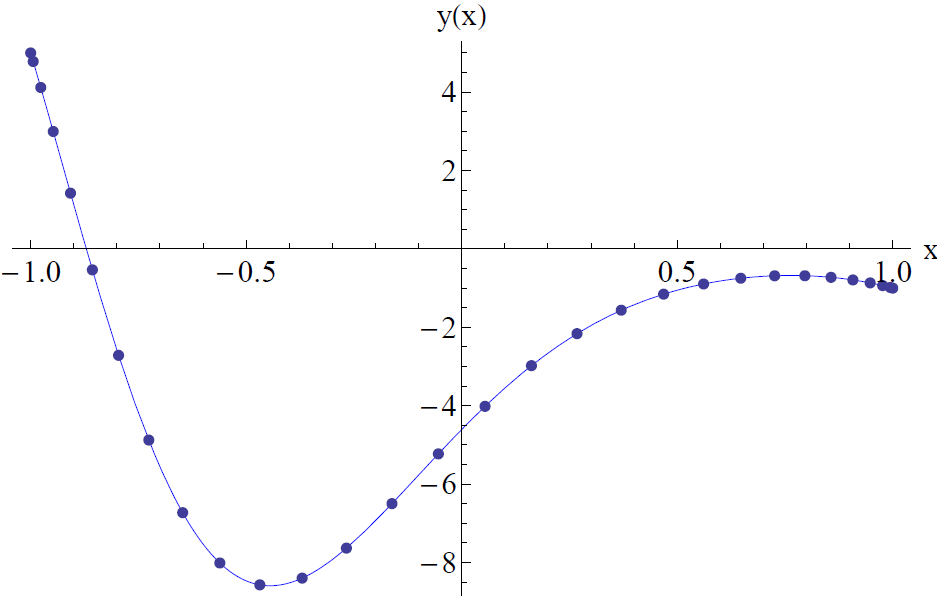
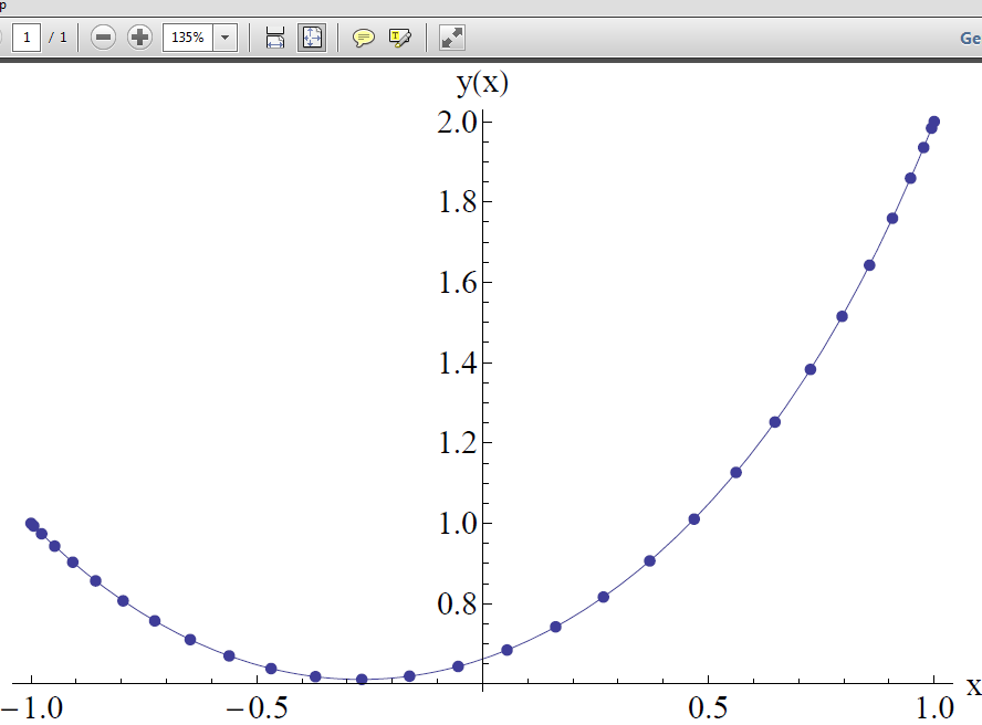
Figure 2.1: The analytic and pseudo-spectral solutions of eqn. 2.2.7 (left) and eqn. 2.2.11 (right), using $n=30$ grid points. Both require only a few fast matrix inversions, and obtain solutions accurate to 19 and 15 digits respectively.

2.2.4 Thermalisation criterion

In this homogeneous setting there is no momentum flow by symmetry, and hence there are no hydrodynamic modes. Alternatively one can say that all gradients vanish, and hence the hydrodynamic stress tensor 1.3.1 equals its ideal part. This means that in this particular case the applicability of hydrodynamics (hydrodynamisation) is equivalent to an isotropic plasma with $\Delta\mathcal{P}(t)=0$.

Although $\mathcal{E}$ is constant in time, the physical temperature can only be assigned to the system once the equilibrium is reached. In this regime $\mathcal{E}=3\pi^{4}T^{4}/4$ and the metric takes the form

$$ds^{2}=2dtdr-r^{2}\left(1-\frac{(\pi T)^{4}}{r^{4}}\right)dt^{2}+r^{2}d\vec{x}^{2}\,,$$ (2.2.14)

or in terms of $A$, $S$ and $B$

$$A=r^{2}\left(1-\frac{(\pi T)^{4}}{r^{4}}\right),\quad S=r\quad\mathrm{and}\quad B=0,$$ (2.2.15)

and describes the Schwarzschild-AdS solution between the boundary and the future event horizon covering also the black brane interior.

Although equilibration of a holographic system can be sampled with different field theory probes, including expectation values of local operators, two point functions, entanglement entropy and Wilson loops, in this study we will primarily focus on tracing the evolution of the one-point function of the stress tensor. There are two reasons for this. In the first place this is the quantity of interest if one wants to make a phenomenological contact with the fast applicability of hydrodynamics at RHIC and LHC. Secondly, after the stress tensor eventually settles down to its thermal value, the geometry becomes a patch of the Schwarzschild-AdS black brane and from this moment on there is no need to evolve the Einstein’s equations further.

We will hence define thermalisation time as the isotropisation time $t_{\text{iso}}$, i.e. the time after which the stress tensor anisotropy $\Delta\mathcal{P}(t)$ remains small compared to the energy density and eventually decays to zero. In our calculations, as in [57], we adopt the following criterion for $t_{\text{iso}}$:

$$\Delta\mathcal{P}(t>t_{\text{iso}})\leq 0.1\,\mathcal{E},$$ (2.2.16)

but it is important to keep in mind that thermalisation is never a clean-cut event and the threshold on the RHS of (2.2.16) can be always slightly raised or lowered without altering much the results. Note that in later chapters (subsection 3.1.4) we will analogously define $t_{\text{hyd}}$ in non-homogeneous settings, but then $\Delta\mathcal{P}$ is given by the difference between the real pressure and the pressure computed within hydrodynamics.

2.2.5 Numerical implementation - Einstein equations

In the numerical implementation instead of the variable $r$ we used its inverse

$$z=1/r,$$ (2.2.17)

so that the AdS boundary is at $z=0$. We furthermore chose units $a_{4}=-1$ and $\xi(t)=0$, such that the horizon of the final black brane will be located at $z=1$, which can be seen from eqn. 2.2.14 with $a_{4}=\pi T^{4}.$ Note however that, for definiteness, all dimensionful quantities that we will provide will be specified in terms of the energy density or, equivalently, the temperature of the final black brane, which is the only scale at the moment of thermalisation.

The Einstein equations 2.2.5 and the functions $A(z,\,t)$ and $S(z,\,t)$ diverge at the boundary. For numerics one could in principle solve this problem by multiplying the Einstein equations with the right power of $z$, and redefining $A(z,\,t)\rightarrow A(z,\,t)z^{2}$ and $S(z,\,t)\rightarrow S(z,\,t)z$. This, however, is not the most effective way of solving the equations, as all dynamics take place at the order of the normalisable modes $b_{4}(t)$ and higher order. The leading order behaviour near the boundary is solely governed by the non-normalisable modes, which are fixed and therefore known analytically.

This leads us to propose to rewrite all equations and functions in 2.2.5 such that they are both finite and non-trivial at the boundary (with the possible exception of $S$). Although this strategy may make the equations somewhat longer, it has the advantage of directly computing the quantity we are interested in. In practice this leads to the following redefinitions:

$$z^{4}\tilde{B}=B,\quad z^{4}\tilde{S}=S-1/z,\quad z^{2}\tilde{A}=A-1/\,z^{2},\quad z^{3}\tilde{\dot{B}}=\dot{B},\quad z^{2}\tilde{\dot{S}}=\dot{S}-1/2z^{2},$$ (2.2.18)

where we then solely compute with $\tilde{B}$, $\tilde{S}$, $\tilde{A}$, $\tilde{\dot{B}}$ and $\tilde{\dot{S}}$. As an example, eqn. 2.2.5a is rewritten into:

$$\left(2\,z^{2}\,\partial_{z}^{2}+20\,z\,\partial_{z}+\left(z^{8}\left(z\,\partial_{z}\tilde{B}+4\tilde{B}\right)^{2}+40\right)\right)\tilde{S}=-z^{3}\left(z\,\partial_{z}\tilde{B}+4\tilde{B}\right)^{2}\,.$$ (2.2.19)

This equation reduces to $\tilde{S}=0$ in the limit $z\rightarrow 0$, which in this case means that the boundary condition is already included at the grid point $z=0$ and does not need to be imposed explicitly. This contrasts somewhat with the idea that any differential equation needs explicit boundary conditions, but in this example all homogeneous solutions of $\tilde{S}$ actually diverge and are therefore put to zero already when expanding in Chebyshev polynomials (eqn. 2.2.10).

Unlike equation 2.2.19, some equations will contain explicit $1/z$ terms, prohibiting a direct evaluation at $z=0$. To resolve this we expand all equations near $z=0$ and treated this point separately. Using these rewritten Einstein equations it is then possible to obtain $\partial_{t}\tilde{B}$ and one can proceed to the next time step, where we use a $4{}^{\text{th}}$ order Adams-Bashforth stepper:

$$\tilde{B}_{n+4}=\tilde{B}_{n+3}+\Delta t\left(\tfrac{55}{24}\partial_{t}\tilde{B}(t_{n+3})-\tfrac{59}{24}\partial_{t}\tilde{B}(t_{n+2})+\tfrac{37}{24}\partial_{t}\tilde{B}(t_{n+1})-\tfrac{3}{8}\partial_{t}\tilde{B}(t_{n})\right)$$ (2.2.20)

The first five time steps are done using smaller and increasing time steps, solving for the next $\tilde{B}$ using Mathematica’s Interpolation and Integration routines. Typically, we use time steps of size $\Delta t=0.0025\sim 1/n^{2}$.

As a way of monitoring the accuracy of our code, we used the normalised constraint (2.2.5e)

$$\kappa(t)=\mathrm{max}_{\,r}\left(\frac{\ddot{S}+\frac{1}{2}\dot{B}^{2}S-\frac{1}{2}A^{\prime}\dot{S}}{|\ddot{S}|+\frac{1}{2}\dot{B}^{2}S+\frac{1}{2}|A^{\prime}\dot{S}|}\right)\Bigg{|}_{\mathrm{fixed}\,\,t}$$ (2.2.21)

The convergence of our code is then illustrated by Fig. 2.2, which shows typical plots of the maximum value of the normalised constraint $\kappa(t)$.

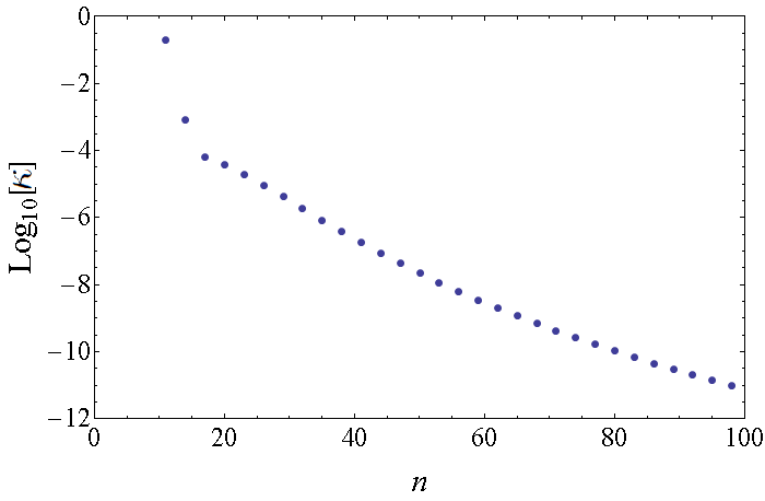
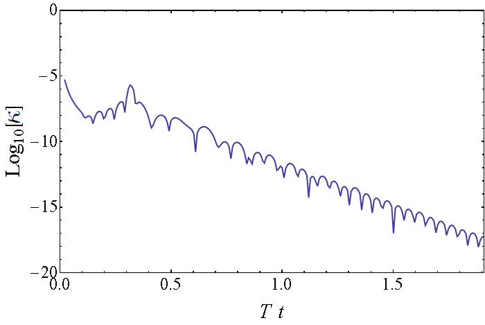
Figure 2.2: The left plot shows the value of the normalised constraint $\kappa(t=0)$ as a function of the number of grid points $n$ for the evolution of the initial profile $B(z,\,t_{\text{ini}})=\frac{8}{3}\mathcal{E}z^{4}$. It is clear from the plot that our numerics converges exponentially with the number of grid points. The right plot shows the evolution of $\kappa(t)$ as a function of time for $n=26$ and one can see there that the constraint actually decreases with time. To achieve $\kappa(t)<10^{-9}$ one typically needs higher precision than the standard double precision computations offer.

The last feature that needs to be discussed is the choice of the position of the inner boundary of the computational grid. Note that the simulation is well defined only if the grid covers the entire portion of the spacetime outside the event horizon. Initially this is hard to predict, since the position of the event horizon depends on the future evolution. Therefore one typically focuses attention on the presence of the apparent horizon because, if it can be found, it is guaranteed to lie inside the black hole. However, quite frequently in our case there is no apparent horizon on the initial-time slice and therefore we use the following procedure. We first try to run simulations with the radial cut-off put at $z=1.01$, which is right below the late-time position of the event horizon. This often works, and when it does not we rerun the simulation with $z=1.07$ as a cut-off. The latter point turns out to almost always lie past the event horizon. In this way we can successfully evolve a large number of initial states.

As a simple example we present two specific evolutions in figure (2.3) with initial $B(z)$ given by

$$B_{\text{ini}}(z)=3\mathcal{E}\,z^{4}\>\text{and }B_{\text{ini}}(z)=(\frac{4}{3}\mathcal{E})^{6}z^{24}.$$ (2.2.22)

The first has the anisotropy located at all scales, whereas the latter is focussed in the infrared. We will come back to the surprising finding that the linearised approximation (purple lines) performs so well, even for these almost maximally far-from-equilibrium states (section (2.3)).

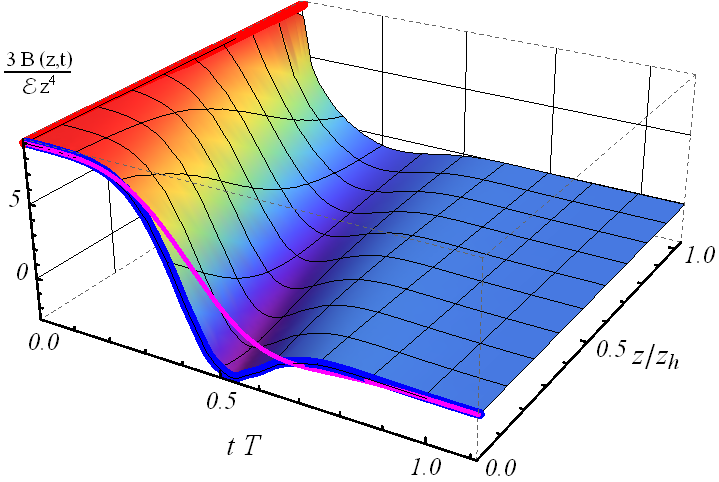
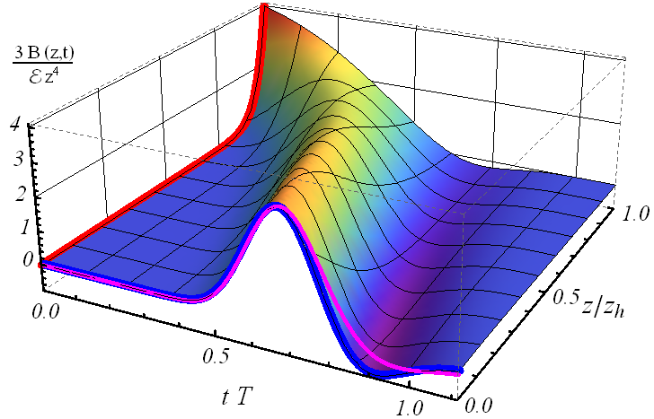
Figure 2.3: The left plot shows $B(z,\,t)$ for the first initial of profile (2.2.22), which is shown as a thick red line at $t=0$. The thick blue curve at $z=0$ shows the value of the gauge theory quantity $\Delta\mathcal{P}(t)/\mathcal{E}$. The purple line shows the linear approximation, explained in subsection 2.3.1. The right plot (second profile in (2.2.22)) shows similar behaviour. The initial disturbance, which is localised in the IR part of the geometry, propagates to the boundary in a time limited by causality. This creates the pressure anisotropy, which quickly relaxes back to zero.

2.2.6 The event and apparent horizons and their entropy

The event horizon is defined as the causal boundary of the black hole. It is a teleological object which can be located only after the black hole settles down to the state of permanent equilibrium. The apparent horizon is defined as the outermost surface where outgoing light rays are trapped, i.e. any causal evolution of the surface decreases in area.

We will be interested in the area of these horizons as examples of easy-to-compute bulk observables that are directly sensitive to the form of the geometry in the deep IR. Although no precise definition of the entropy density exists in a truly far-from-equilibrium situation, the change in the area density of these horizons provides a crude measure of the total entropy produced in the thermalisation process. For this reason we will loosely refer to the area density of these horizons as ‘entropy density’, but we emphasise from the start that this terminology is rigorously applicable only near equilibrium. In equilibrium both horizons are indeed equal, but this is not the case during the far-from-equilibrium regime; indeed we even found many evolutions with no apparent horizon in the initial time slice at all.

In our homogeneous setting the event horizon will be a hypersurface defined by

$$r-r_{\text{EH}}(t)=0,$$ (2.2.23)

with the normal vector being null

$$r_{\text{EH}}^{\prime}(t)-\frac{1}{2}A\left(t,r_{\text{EH}}(t)\right)=0.$$ (2.2.24)

The latter is the geodesic equation for the outgoing light ray and needs to be supplemented with the following condition to be imposed in the asymptotic future

$$r_{\text{EH}}(t)\rightarrow\pi T\quad\mathrm{as}\quad t\rightarrow\infty\,.$$ (2.2.25)

In practical terms this condition implies that when the metric eventually approaches the form of the Schwarzschild-AdS black brane (2.2.14), $r_{\text{EH}}$ approaches the position of the event horizon of the static solution. The apparent horizon in a homogeneous setting can be found by solving the algebraic equation $\dot{S}(t,r_{\text{AH}}(t))=0$, but see subsection (3.1.2) for a more non-trivial example in a non-homogeneous setting.

The area (3 dimensional) of both horizons gives rise to the following expression for the entropy density:

$$s_{\text{EH/AH}}(t)=\frac{1}{2\pi}N_{c}^{2}\,S\left(t,\,r_{\text{EH/AH}}(t)\right)^{3},$$ (2.2.26)

which for the event horizon is guaranteed to be a non-decreasing function of $t$. In (2.2.26) we implicitly assume that a horizon is mapped onto the boundary along ingoing null radial geodesics, i.e. along lines of constant $t$ for the metric ansatz (2.2.1).

In figure (2.4) the horizon areas are plotted for the example profile of figure 2.3. Indeed there is no initial apparent horizon, although in our AdS setting there will always be a (small) event horizon. From this figure it is very clear that this profile starts out far-from-equilibrium, since the black hole area grows more than a factor of 3.

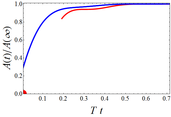
Figure 2.4: Time evolution of the areas of the event (blue) and apparent (red) horizons for the initial state of figure (2.3). The red dot at the origin signifies that there is no apparent horizon for this state at the initial time. From that time until the start of the red curve there is no apparent horizon within the range of the radial coordinate covered by our grid, but there could be one at a deeper position.

2.2.7 A sample profile and expectations for thermalisation times

To get intuition about how the dynamics proceeds on the gravity side and to get acquainted with the features following from the choice of a foliation by null constant-time slices, it will be instructive to discuss in detail the dynamics of the following initial state

$$B(t=0,z)=\frac{2}{15}\mathcal{E}\,z^{4}\exp\left[-\frac{150}{z_{h}^{2}}\left(z-\tfrac{1}{3}z_{h}\right)^{2}\right]\,,$$ (2.2.27)

where $z_{h}=\frac{2^{1/2}}{3^{1/4}}\mathcal{E}^{1/4}$. As $B$ is supported at intermediate values of $z$, naive intuition from the physics of linear wave equations would suggest that the wave packet splits into two: one propagating inwards and the other propagating outwards. The one propagating outwards is expected to eventually reach the boundary, bounce back and fall into the bulk. Both wave packets will be eventually absorbed by the event horizon (which is guaranteed to be present given that $\mathcal{E}\neq 0$) leading to the increase in its area.

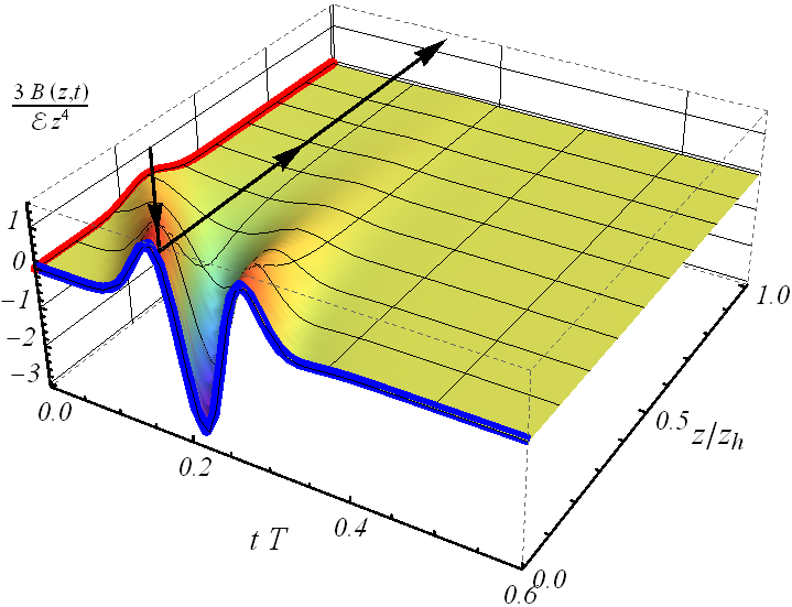
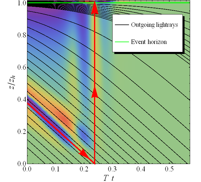
Figure 2.5: The left figure shows $B$ as a function of time and radial coordinate for the initial profile (2.2.27), which is shown as a thick red curve at $t=0$ and which is initially localised near $z=\tfrac{1}{3}z_{h}$. The blue curve at the boundary ($z=0$) depicts the pressure anisotropy as a function of time in the gauge theory. The right figure shows the Kretschmann scalar (with the value for an equilibrium black brane with the same energy density subtracted) as a function of time and radial coordinate for the same initial profile. One clearly sees on this plot the wave bouncing off the boundary and falling into the black brane. In the adopted generalised ingoing Eddington-Finkelstein coordinates this happens instantaneously.

These expectations are confirmed by the outcome of the numerical simulation, as illustrated by Fig. 2.5, which depicts the bulk anisotropy (left plot) and the square of the Riemann tensor, the Kretschmann scalar (right plot). We can clearly see the rise in the curvature due to the outgoing wave packet as it approaches the boundary of AdS. Closer inspection reveals also the presence of a wave packet resulting from the bouncing off the boundary of the outgoing packet. This wave packet, due to the null nature of our coordinate frame, propagates towards the boundary from the horizon along lines of constant Eddington-Finkelstein time. Note also that this signal falls through the black brane event horizon without significant scattering. This feature persisted for other choices of initial states and seems to be related to the high degree of symmetry of our problem.

It is interesting to note that the initial ingoing part of the wave packet seems to be mostly taken care of by the solution of the constraints. Indeed, although $B$ is supported only over some small range of $z$ centred around $z_{h}/3$, the metric functions $A$ and $S$ deviate from their vacuum values all the way from this point to the horizon, as required by causality. In contrast, the curvature outside the outgoing wave packet is very close to the curvature of the static black brane.

These observations suggest that the states which take the longest time to thermalise are those that are initially localised close to the horizon on the initial-time slice. An example is provided by $B(t=0,z)\sim z^{24}$, whose evolution is shown in figure 2.3 (right). The reason is that the outgoing wave packet needs to escape the neighbourhood of the horizon and travel all the way to the boundary to bounce off and finally fall into the black brane horizon. By localising the initial profiles close to the horizon, the longest isotropisation times that we are able to obtain with our numerics, which uses rather moderate grids, are about $1.1/T-1.2/T$, with $T$ the final equilibrium temperature (see figure 2.10).

2.3 A large sample of states and a linearised simplification

Apart from toy-models based on the AdS-Vaidya geometry of infalling dust (see e.g. [58, 59, 60, 61], but also [62]), the only existing approximation scheme to study holographic thermalisation processes is the amplitude expansion, in which one linearises Einstein’s equations on top of the static black brane background. In this approximation the relaxation towards equilibrium is described by quasinormal modes with complex frequencies, whose imaginary parts lead to the damping of their amplitudes with time and hence to equilibration. These modes were thought so far to be appropriate for the description of only the late-time approach to equilibrium, when deviations from equilibrium are sufficiently small in amplitude [37].

An indication that this assumption might be too restrictive comes from black hole mergers in asymptotically flat four-dimensional spacetime. There, in the so-called close-limit approximation, the Einstein’s equations linearised on top of the final black hole predict rather accurately the pattern of gravitational radiation at infinity provided the initial data have a single horizon surrounding the merging black holes [63, 64]. This initial horizon, however, needs not to be a small perturbation of the final black hole for the close-limit approximation to work.

These features, together with the observation that the AdS analogue of gravitational radiation at infinity is the expectation value of the boundary stress tensor, motivates us to apply a linear approximation to the simple example of far-from-equilibrium gravitational dynamics in AdS spacetime studied above. With the algorithm to generate many initial states (subsection (2.2.2)) we can then compare the full numerical solution of the Einstein equations with the one linearised on top of the black brane background. Quite surprisingly, even for states which we found to be maximally far from equilibrium, the linearised approximation always works within about 20%. This finding can therefore greatly simplify future computations.

2.3.1 Leading order correction to the pressure anisotropy

Linearising Einstein’s equations in the setup of holographic isotropisation can be formally phrased as an expansion in the amplitude of perturbations on top of the Schwarzschild-AdS black brane. We thus write

$$A(t,z)=\frac{1}{z^{2}}(1-z^{4})+\alpha\,\delta A(t,z) + \mathrm{\mathcal{O}}(\alpha^{2}),$$

$$S(t,z)=\frac{1}{z}+\alpha\,\delta S(t,z)+\mathcal{O}(\alpha^{2})\quad\mathrm{and}\quad B(t,z) = \alpha\,\delta B(t,z)+\mathcal{O}(\alpha^{2}),$$ (2.3.1)

where $\alpha$ is a formal parameter counting the order in the amplitude expansion.

The smallness of the initial data can be physically quantified by either measuring the total entropy production on the event horizon or by following the amplitude of the pressure anisotropy during the evolution process and comparing it to the energy density. It is important to re-stress that we want to use the linearised approximation without necessarily restricting to the initial data being small perturbations of the Schwarzschild-AdS black brane, precisely in the spirit of the original close-limit approximation [63, 64] but now in the context of AdS spacetime.

The initial data for the full non-linear Einstein’s equations are given by specifying the energy density $\mathcal{E}$ and the form of $B$ as a function of the radial coordinate on the initial-time slice. As anticipated earlier, one of the motivations for choosing $B$ over $S$ in specifying the initial data was that the former appears quadratically in the constraint (2.2.5a). This feature persists also with the other components of the Einstein equations apart from the equation (2.2.5c), which immediately leads to

$$\delta A(t,z)=0\quad\mathrm{and}\quad\delta S(t,z)=0.$$ (2.3.2)

$\delta B(t,z)$ on the other hand remains nontrivial and is a solution of the equation (2.2.5c) with $A$ and $S$ set to their form in the Schwarzschild-AdS background given in (2.2.15).

The initial condition for this equation is the same as the initial condition for the full Einstein’s equations, i.e.

$$\delta B(t=0,z)=B(t=0,z).$$ (2.3.3)

The energy density $\mathcal{E}$, which is constant in our setup and is the remaining part of the initial state specification, is already included in the background that we linearise on top of.

In full detail, the equation for $\delta B(t,z)$ reads (with the choice of units $\mathcal{E}=\frac{3}{4}$)

$$\frac{1}{2z}(3+z^{4})\,\partial_{z}\delta B-\frac{1}{2}(1-z^{4})\,\partial_{z}^{2}\delta B-\frac{3}{2z}\,\partial_{t}\delta B+\partial_{z}\partial_{t}\,\delta B=0\,.$$ (2.3.4)

2.3.2 Connection with quasinormal modes

Equation (2.3.4) can be solved either as an evolution equation given some initial profile for $\delta B$, as discussed in the previous section, or by decomposing $\delta B$ as a superposition of modes with factorised time dependence:

$$\delta B(t,z)\sim e^{i\omega_{j}t}\,b_{j}(z).$$ (2.3.5)

These modes are known as quasinormal modes, and they are characterised by the requirements that they are normalisable near the boundary ($z=0$) and that they obey in-going boundary conditions at the event horizon ($z=1$). The latter condition makes the frequencies $\omega_{j}$ complex with imaginary parts responsible for the exponential decay in time. The quasinormal modes (2.3.5) appear in pairs, as taking the complex conjugate of the equation (2.3.4) for the quasinormal mode with frequency $\omega_{j}$ leads to the equation for the quasinormal mode with frequency $-\omega_{j}^{*}$. This feature can be seen in figure 2.6.

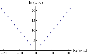
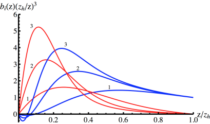
Figure 2.6: The plot on the left shows the frequencies of the ten lowest quasinormal modes including their complex conjugates. The mode with the smallest negative imaginary part will be the dominant mode at late times. Notice that the spacing between the modes is approximately constant (it differs by about 0.1%). The plot on the right displays the lowest three quasinormal modes as a function of the radial coordinate $z$, where blue and red denote their real and imaginary parts. The normalisation we use is such that the real part at the horizon ($z/z_{h}=1$) is equal to unity, whereas the imaginary part vanishes there. One clearly sees that higher modes (which decay faster) are more dominant near the boundary.

In the context of gravitational collapse, the lowest quasinormal modes are known to govern the late-time decay of black hole perturbations (see e.g. [66]) and this is also expected in the current setup. On the other hand, the results from [57], reviewed in the previous section, suggest that the equation (2.3.4) predicts the full time dependence of the large-$z$ behaviour of function $B$ rather well. Hence it is a natural question to compute the quasinormal mode content of the perturbations that we considered.

In order to answer this question we followed the prescription of [37] and computed the lowest 10 quasinormal modes (2.3.5) by solving equation (2.3.4) for the ansatz (2.3.5) in the near-horizon expansion and evaluating the resulting expression at the boundary to find $\omega_{j}$’s leading to normalisable modes. The (somewhat arbitrary) normalisation of our modes is fixed by demanding that at the horizon $(z=1)$

$$b_{j}(1)=1.$$ (2.3.6)

On figure 2.6 we plot the obtained frequencies $\omega_{j}$ of the lowest 10 quasinormal modes, as well as bulk profiles for the real and imaginary parts of $b_{1}(z)$, $b_{2}(z)$ and $b_{3}(z)$ normalised according to (2.3.6).

 

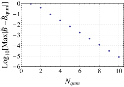
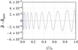
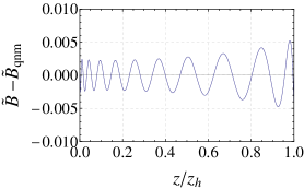
Figure 2.7: The plot on the left displays the maximum of the error when approximating $\tilde{B}(z)=B(z)/z^{3}$ by the first $N_{\text{QNM}}$ (complex) quasinormal modes, with $B(t=0,z)=-2a_{4}z^{4}$. The plot in the middle shows the error for the same profile as a function of the bulk coordinate $z$ while using the 10 lowest quasinormal modes. The right plot displays the error for $B(t=0,z)=z^{25}$ and shows clearly that a profile which is dominated in the IR is much harder to fit by the quasinormal modes. This causes oscillations in the evolution, as can be seen in figure 2.9.

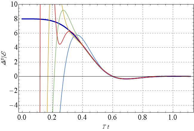
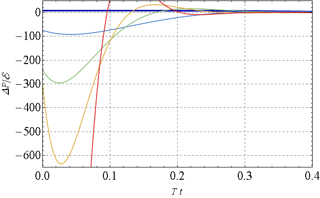
Figure 2.8: On the left one sees the pressure anisotropy $\Delta\mathcal{P}/\mathcal{E}$ as predicted by the linearised evolution, or indistinguishably by the sum of the lowest 10 quasinormal modes as a thick blue line. One can also see there the sum of the first 1 (blue), 2 (green), 3 (orange) or 4 (red) quasinormal modes. As becomes apparent, the late time dynamics is well approximated already by keeping only the lowest quasinormal mode, but if one uses more the fit starts matching earlier. Note that the coefficients are computed such that the sum of the 10 fits the initial state best.
On the right we plot the individual quasinormal modes with the same coloring. One clearly sees that each of them carries very large anisotropy, but that their interference matches the linearised solution.

The idea now is to use the quasinormal modes to decompose solutions of (2.3.4), i.e. to write a solution of (2.3.4) in the form

$$\delta B_{\text{QNM}}(t,z)=\text{Re}\left[\underset{i=1}{\overset{N_{\text{QNM}}}{\sum}}c_{i}\,b_{i}(z)\,e^{i\omega_{i}t}\right],$$ (2.3.7)

where we truncated the expansion at some $N_{\text{QNM}}$, although formally we could set $N_{\text{QNM}}=\infty$. In our calculations we used $N_{\text{QNM}}=10$.

One can view (2.3.7) as a further simplification as compared with solving numerically (2.3.4), which approximates the full Einstein’s equations well. The reason for this extra simplification is that now the solution is specified by providing a few complex numbers (say 10 complex coefficients $c_{j}$’s) which due to the linearity of the problem can be fitted on the initial-time slice to $B(t=0,\,z)$.

As a way of generating coefficients $c_{j}$’s we minimised

$$\int_{0}^{1}\frac{dz}{z^{3}}\left|B(t=0,z)-\delta B_{\text{QNM}}^{(1)}(t=0,z)\right|$$ (2.3.8)

by using the least squares method on a discrete sample of the radial position $z$. Naturally, one needs far more points than the number of quasinormal modes included in (2.3.7).

The subtlety in using (2.3.8) lies in the choice of the multiplicative factor under the integral, which we set to be $1/z^{3}$. We checked that both $1/z$ and $1/z^{4}$ do not work well, as the first one does not take sufficiently into account and the other overcounts the near-boundary behaviour of $B(t=0,z)$. On the other hand, $1/z^{2}$ seems to work equally well as $1/z^{3}$, but for definiteness we focused here on the latter.

Figure 2.7 displays the difference between $B(t=0,z)$ and $\delta B_{\text{QNM}}(t=0,z)$ as a function of the number of quasinormal modes in two representative examples. Clearly, if a good fit is possible, then the profile (2.3.7) will solve the linearised Einstein’s equations nicely since each quasinormal mode solves them individually.

In figure 2.8 we compare the linearised evolution obtained from a direct solution of (2.3.4) and from a solution based on a decomposition into quasinormal modes. One can see that the contribution from each individual quasinormal mode can be large, but that the final sum approximates the linearised evolution very well. Finally, in figure 2.9 we plot three representative examples, where the profile with $B(t=0,z)$ having support mostly in the IR displays this interference phenomenon particularly nicely.

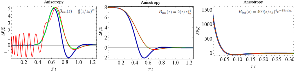
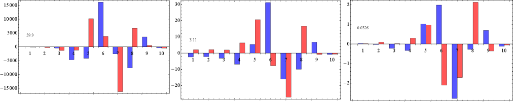
Figure 2.9: In this figure we illustrate anisotropies of the full (blue), linearised (green) and quasinormal mode (red) evolution of three representative initial profiles, located in the IR, spread-out and located in the UV respectively. Clearly, the initial profile located in the IR takes some time before exciting the anisotropy at the boundary, which also explains the late thermalisation. The UV profile can have a very large anisotropy, but isotropises very fast.
These features are nicely described when looking at the quasinormal modes coefficients $c_{j}$’s (below, real (blue) and imaginary (red) part). For the IR profile each individual contribution is very large, but they interfere in such a way to give only moderate anisotropies. In this way it is also possible to reach isotropisation as late as 6 times the lowest QNM e-folding time. We also see that one would need to compute more quasinormal modes to accurately fit this profile.

The interference described above is important to counter a naive argument about a bound on the thermalisation time. Naively one may argue that a state with a maximal thermalisation time should consist fully of the lowest quasinormal mode, as this mode decays the slowest. According to the argument in subsection (2.2.2) the amplitude of this mode should be bounded to avoid a naked singularity, which would then imply a bound on the thermalisation time. That this argument fails is clear from figure 2.8: each individual mode would lead to a naked singularity, but the sum is perfectly well behaved. In fact, this leads us to believe that a profile located as close as possible to the event horizon could have an unbounded thermalisation time, though it is probably exponentially hard to obtain larger and larger thermalisation times.

This in principle unboundedness of the thermalisation time fits well with causality in the field theory: if one starts with a state having large correlations over a distance $\ell$, causality demands thermalisation times bigger than $\ell/2$. The current section and arguments above suggest that in a strongly coupled theory such states are very fine tuned and more importantly they will still thermalise fast, in a time close to the bound by causality.

2.3.3 Holographic isotropisation simplified

The main motivation for studying holographic thermalisation is learning possible lessons about the way the thermalisation (or rather hydrodynamisation) process proceeds in relativistic heavy ion collisions at RHIC and LHC. For this we compare over a 1000 different initial states and found that the full Einstein equations always lead to an isotropisation time $t_{\text{iso}}$ less than $1.2/T$, with $T$ the final temperature of the plasma. Furthermore, we compare all these profiles with their linearised approximation, and find that the difference in thermalisation times $\Delta t_{\text{iso}}=t_{\text{iso}}-t_{\text{iso, lin}}$ is almost always less than $20\%$ of $t_{\text{iso}}$. These findings are summarised in the histogram of figure (2.10).

By replacing QCD by a theory with a gravity dual one only expects to obtain either qualitative insights or quantitative ball-park estimates [67]. In this sense a $20\%$ accuracy is more than what is needed in order to understand the phenomena we are interested in, and at the same time may allow to address otherwise technically hard-to-tackle questions. Two examples of such problems in the relativistic heavy ion collisions context are the pre-equilibrium phase of the elliptic flow and the equilibration of transverse-plane inhomogeneities following from event-by-event fluctuations. Solving their holographic analogues in full generality will require complicated simulations of AdS-black hole spacetimes depending on all five bulk coordinates and our hope is that a suitably developed linear approximation may allow us to obtain results with a reasonable accuracy at a much smaller cost.

The most important open problem is if our linearised simplification extends to more non-trivial cases where the final state will not be known in advance. Preliminary results in expanding boost-invariant plasmas suggest that this is indeed the case, provided one takes care to chose a proper fiducial state to linearise around. This suggests interesting opportunities to linearise around more non-trivial backgrounds, such as presented in the next two chapters.

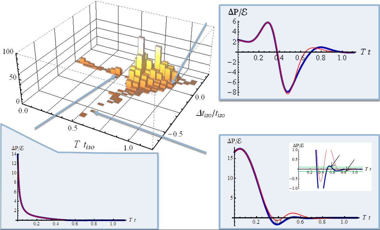
Figure 2.10: The histogram plots the isotropisation time $t_{\text{iso}}$ versus the difference between the isotropisation time predicted by the full and the linear equations, $\Delta t_{\text{iso}}$. The height of each bar in the histogram indicates the number of initial states for which the evolution yields values in the corresponding bin. The total number of initial states is more than 1000. We see both that holographic isotropisation proceeds quickly, at most over a time scale set by the inverse temperature, and that the linearised Einstein’s equations correctly reproduce the isotropisation time with a 20% accuracy in most cases. A close inspection of one of the few profiles (bottom right) for which the linearised approximation seemingly fails by more than 20% ($\Delta t_{\text{iso}}/t_{\text{iso}}=-0.5$) shows that it is the imperfect isotropisation criterion which leads to the mismatch rather than the failure of the linear approximation. Indeed, the plot shows that, on the scale of the initial anisotropy, the linear result yields a good approximation. However, the isotropisation criterion makes no reference to this scale, and results in a 50% difference in the isotropisation times, indicated by the arrows on the small plot. See [52] for a related discussion of subtleties involved in defining the thermalisation (or more accurately hydrodynamisation) time in a similar setup.

Chapter 3 Colliding planar shock waves in AdS

This chapter presents two studies [68, 69] of colliding shocks in AdS, which can provide insights in the longitudinal dynamics in heavy-ion collisions (HIC) in the first far-from-equilibrium regime. These shocks are constructed such that the field theory stress-tensor before the collision provides a good model for real heavy-ion collisions. Although event-by-event fluctuations presumably make transverse dynamics important, this chapter is limited to shocks homogeneous in the transverse plane.

Gravitational shock waves were first studied in [70], where they considered boosting a Schwarzschild metric of mass $m$ with a velocity $v$. The shock wave metric can then be obtained by taking the limit $v\rightarrow 1$, keeping the total energy, $\gamma m=(1-v^{2})^{-1/2}m$ fixed. Because of Lorentz contraction, it was found that the metric was flat everywhere, except on the plane transverse to the direction of motion.

Our shock waves are somewhat different; they move in 5 dimensional AdS, are planar in the transverse field theory coordinates, can have non-trivial structure in the longitudinal direction and do not contain explicit sources. On the other hand, they can still be thought of as a boosted source, where the limit is taken of a very energetic source very far away, such that the profile in this limit is indeed homogeneous in the transverse plane.

Perhaps more intuitively, one can think of the shock waves from a field theory perspective. The shock waves are then defined by an energy density $\mathcal{E}(x_{L},\,\vec{x}_{T})$ at some moment in time and after which we demand that this energy density moves at the speed of light. This completely fixes the AdS geometry in the case of pure gravity without sources.

This chapter is accompanied by the notebook/package ‘shockwaves.nb’. The notebook contains all details of the computations presented and for ease of use there are a few sample notebooks to run a simulation and interpret the results. Note that the package includes the electromagnetic field and can hence also collide charged shock waves. Details of those computations are not part of this chapter, which deals with pure gravity only.

3.1 Solving Einstein’s equations

The evolution of Einstein’s equations can be conveniently done using the method described in sections 2.1 and 2.2, first described in [39]. For this we need to write the metric in the form 2.1.1, which given the planar symmetry in the transverse plane reduces to

$$ds^{2}=dt(2dr-Adt+2Fdz)+S^{2}(e^{B}d\mathbf{x}_{\perp}^{2}+e^{-2B}dz^{2}),$$ (3.1.1)

where all functions now depend on $r,\,t,$ and $z$. Similar to the homogeneous case initial conditions are given by $B(r,\,t_{0},\,z)$, $a_{4}(t_{0},\,z)$ and $f_{4}(t_{0},\,z)$, where the latter two are defined by the near-boundary expansions:

$$\begin{array}[]{cccccc}A(r,\,t,\,z)&=&(r+\xi)^{2}-2\partial_{t}\xi+\frac{a_{4}}{r^{2}}+O\left(r^{-3}\right),&B(r,\,t,\,z)&=&\frac{b_{4}}{r^{4}}+O\left(r^{-5}\right),\\ S(r,\,t,\,z)&=&r+\xi+O\left(r^{-5}\right),&F(r,\,t,\,z)&=&\partial_{z}\xi+\frac{f_{4}}{r^{2}}+O\left(r^{-3}\right),\end{array}$$ (3.1.2)

where also $b_{4}$ and the gauge $\xi$ depend on $t$ and $z$, and are undetermined by a near-boundary expansion. In the next subsection we will use the gauge $\xi=0$ to compute the initial conditions, but during the evolution the gauge freedom will be used to fix the location of the apparent horizon at $r=1$ (see subsection 3.1.2).

Transforming the near-boundary expansion above to Fefferman-Graham coordinates (eqn. 2.1.3) we use holographic renormalisation (section 2.1.1) to find the following energy density, energy flux, longitudinal pressure and transverse pressure of the boundary field theory:

$$\langle(-T_{t}^{t},\,T_{t}^{z},\,T_{z}^{z},\,T_{\mathbf{x}_{\perp}}^{\mathbf{x}_{\perp}})\rangle\equiv(e,\,s,\,P_{L},\,P_{T})=\frac{1}{4\pi G_{N}}(-\frac{3}{4}a_{4},\,f_{4},\,-\frac{1}{4}a_{4}-2b_{4},\,-\frac{1}{4}a_{4}+b_{4})$$ (3.1.3)

where all functions depend on $t$ and $z$, and for $\mathcal{N}=4$ SU($N_{c}$) SYM we have $G_{N}=\pi/2N_{c}^{2}$.

To find the Einstein equations suitable for the characteristic method it is essential to understand which function to solve for at each step. Similar to the homogeneous case (subsection 2.2.1), one starts with $B$, solves for $S$ (2), $F$ (2), $\dot{S}$ (1), $\dot{B}$ (1) and $A$ (2), where the numbers indicate the order of the differential equations, which are all ordinary linear differential equations in $r$. Knowing this, it is straightforward to solve the Einstein equations for $S^{\prime\prime}$, $F^{\prime\prime}$, $\dot{S}^{\prime}$, $\dot{B}^{\prime}$, $A^{\prime\prime}$, $\ddot{S}$ and $\dot{F}^{\prime}$, where the latter two are constraints, only used to find the boundary evolution equations

$$\partial_{t}a_{4}=-\frac{4}{3}\partial_{z}f_{4}\text{ and }\partial_{t}f_{4}=-\frac{1}{4}\partial_{z}a_{4}-2\partial_{z}b_{4},$$ (3.1.4)

and furthermore as a useful check on numerical accuracy. The full equations written out can be found either in the Appendix, or the notebook shockwaves.nb.

3.1.1 From Fefferman-Graham to Eddington-Finkelstein

The metric of a single lightlike shock in AdS can be written down analytically in Fefferman-Graham coordinates [71]:

$$ds^{2}=\tilde{r}^{2}(-d\tilde{z}_{+}d\tilde{z}_{-}+d\mathbf{x}_{\perp}^{2})+\frac{1}{\tilde{r}^{2}}(d\tilde{r}^{2}+h(\tilde{z}_{\pm})d\tilde{z}_{\pm}^{2})$$ (3.1.5)

where $\tilde{z}_{\pm}=\tilde{t}\pm\tilde{z}$ and $h(\tilde{z}_{\pm})$ is arbitrary. Below we restrict to left-moving shocks; right-moving shocks follow by symmetry. In order to make use of the efficient characteristic formulation this metric needs to be transformed into the form 3.1.1, which for a left-moving shock can in general be written as

$$\tilde{u}(u,\,t,\,z) = u+a(u,\,t+z),$$

$$\tilde{z}_{+}(u,\,t,\,z) = t+z+b(u,\,t+z),$$

$$\tilde{z}_{-}(u,\,t,\,z) = t-z+c(u,\,t+z),$$

where we changed $\tilde{r}\rightarrow 1/\tilde{u}$. We now have to demand that the transformed metric satisfies

$$g_{uu}=g_{uz}=0,\qquad g_{ut}=-1/u^{2}.$$ (3.1.6)

These equations can be solved algebraically order-by-order near the boundary, leading to the following near-boundary expansion, where we again fixed the gauge freedom $\xi(t,\,z)=0$:

$$\begin{array}[]{ccc}a(u,\,t+z)&=&\frac{1}{6}u^{5}h(t+z)+\frac{1}{10}u^{6}h^{\prime}(t+z)+\frac{1}{30}u^{7}h^{\prime\prime}(t+z)+O\left(u^{8}\right),\\ b(u,\,t+z)&=&u+\frac{1}{15}u^{5}h(t+z)+\frac{1}{30}u^{6}h^{\prime}(t+z)+\frac{1}{105}u^{7}h^{\prime\prime}(t+z)+O\left(u^{8}\right),\\ c(u,\,t+z)&=&u+\frac{7}{15}u^{5}h(t+z)+\frac{1}{3}u^{6}h^{\prime}(t+z)+\frac{9}{70}u^{7}h^{\prime\prime}(t+z)+O\left(u^{8}\right).\end{array}$$ (3.1.7)

With these boundary conditions at hand it would be possible to try and integrate 3.1.6 into the bulk. Although it is possible to get rather accurate results using just Mathematica’s NDSolve, for the shock waves presented below this method is not good enough. One of the difficulties in this system is the divergence at the Poincarï¿œ horizon, at $\tilde{r}=0$, which is a non-trivial function of $t+z$, $u_{hor}(t+z)=-1/a(r,\,t+z)$, in Eddington-Finkelstein coordinates. Solving for $a,$ $b$, and $c$ on a $u$ and $t+z$ (rectangular) grid would therefore fail as soon as $a(u,\,t+z)=-1/u$ for some $t+z$, thereby not giving the complete solution.

Conveniently, eqn. 3.1.6 can be rewritten such that it can be solved locally in $t+z$. This is possible by realising that paths of varying $u$, keeping $t$ and $z$ constant, have to satisfy the geodesic equation for light-rays. In the Fefferman-Graham coordinates the path has the form $x^{\mu}(\lambda)=(\tilde{r}(\lambda,\,t,\,z),\,\tilde{z}_{+}(\lambda,\,t,\,z),\,\tilde{z}_{-}(\lambda,\,t,\,z),\,0,\,0)$, which leads to second order ordinary differential equations, local in $t$ and $z$, for the functions $a$, $b$ and $c$. Their explicit form can be found in the Appendix.

Analogous to subsection 2.2.5 we redefine $a(\lambda)=\tilde{a}(\lambda)\lambda^{5}$ and similarly for $b$ and $c$, such that our variables become finite and non-trivial at the boundary. We solved these modified equations by an $8^{\text{th}}$ order Runge-Kutta stepper, starting at $\lambda=0.03$ with step size $0.002$, where the boundary expansion 3.1.7 (expanded up to order $u^{14}$) provides the boundary conditions.

Having solved the coordinate transformation we can read off $B(t_{0},\,r,\,z)$, which in this case is the only initial condition depending on the full AdS geometry:

$$B(t,\,\lambda,\,z) = \frac{1}{3}\log(g_{x_{\perp}x_{\perp}}/g_{zz})$$ (3.1.8)

$$= -\frac{1}{3}\log\left(\partial_{z}a^{2}+(a+\lambda)^{4}\left(\partial_{z}b+1\right)^{2}h-\left(\partial_{z}b+1\right)\left(\partial_{z}c-1\right)\right).$$ (3.1.9)

This equation depends on space derivatives of $a$, $b$, and $c$, which are obtained by sampling these functions at 7 points around the point where $B$ is to be evaluated. As anticipated, this only works for $\lambda>0.03$, so that for smaller values we used the near-boundary expansion.

The only other initial conditions needed are $a_{4}(t+z)$ and $f_{4}(t+z)$, and the initial conditions for right-moving shocks. The former can again be obtained using the near-boundary expansion, $f_{4}(t+z)=h(t+z)=-\frac{3}{4}a_{4}(t+z)$, and right-moving shocks are obtained by letting $z\rightarrow-z$ and $f_{4}\rightarrow-f_{4}$.

3.1.2 The apparent horizon

Compared to the homogeneous case (section 2.2) the major difference is the non-trivial structure of the (apparent) horizon as a function of $z$. The apparent horizon is defined as the outermost surface with a negative outward expansion rate. Although this definition depends on the time slicing of the spacetime, it has the large advantage over the event horizon that one can compute the horizon locally in time. Probably the easiest way to find the apparent horizon is to compute the outward expansion rate and put it to zero. Here, however, we present a somewhat more physical derivation.

In this derivation it is assumed that the apparent horizon lies at constant $r=r_{h}$, which can always be attained using the gauge freedom $r\rightarrow r+\xi(z)$. The idea is then to shoot outgoing light rays perpendicular from this surface, so that they maximise the surface at a time $t+\delta t$. The apparent horizon is then found by demanding that the surface nevertheless remains constant: the volume inside cannot expand and is trapped.

In a time $\delta t$ the light rays will in general have traveled a distance $\delta r(z)$ in $r$ and $\delta z(z)$ in $z$, but they have to be null:

$$\delta r=\frac{1}{2}\left(\delta t\,A-\frac{\delta z^{2}\,e^{-2B}S{}^{2}}{\delta t}-2\delta z\,F\right).$$ (3.1.10)

The 3-area per transverse 2-area at time $t$ is given by $a(t)\equiv\int dy\sqrt{g_{zz}g_{x_{\perp}x_{\perp}}g_{x_{\perp}x_{\perp}}}=\int_{-\infty}^{z_{f}}S(r,\,t,\,z)^{3}\,dz$ , where we integrate until $z_{f}$ to later find a local formula by varying $z_{f}$. The difference in area density at time $t+\delta t$ is then given by

$$\delta z(z_{f})S(r,t,z_{f})^{3}+\int_{-\infty}^{z_{f}}3S{}^{2}\left(\delta t\,\partial_{t}S+\frac{1}{2}\partial_{r}S\left(\delta t\,A-\frac{\delta z{}^{2}e^{-2B}S{}^{2}}{\delta t}-2\delta z\,F\right)\right)\,dz,$$ (3.1.11)

where all functions have been expanded for small $\delta t$ and $\delta z$ and are now evaluated at $r$, $t$ and $z$. Note also that the integration domain at $t+\delta t$ is changed, which is taken into account by the first term. It is now possible to maximise this difference by extremising over $\delta z$, so that we find

$$\delta z=-\frac{\delta t\,e^{2B}F}{S{}^{2}}.$$ (3.1.12)

Lastly, we put this back in 3.1.11, which gives an apparent horizon if it is zero for all $z_{f}$. The latter is done by differentiating with respect to $z_{f}$ and letting $z_{f}\rightarrow z$, giving

$$3S^{2}\dot{S}-\partial_{z}\left(S\,F\,e{}^{2B}\right)+\frac{3}{2}e^{2B}F^{2}S^{\prime}=0,$$ (3.1.13)

where we furthermore recognised $\dot{S}=\partial_{t}S+\frac{1}{2}AS^{\prime}$, and naturally all functions have to be evaluated at $r=r_{h}$. If the surface is not at constant $r$ the equation remains the same, replacing $F\rightarrow F+\frac{\partial r_{h}}{\partial z}$, $r_{h}$ being the position of the apparent horizon. For this replacement one can repeat the whole derivation, but alternatively one can realise that the horizon is at constant $r_{h}$ for an appropiate gauge $\xi(z)$ (note that eqn. 3.1.13 explicitly does not depend on $\partial_{t}\xi$). Eqn. 3.1.13 then becomes a second order non-linear equation for $\xi$ (note that $F$ depends on $\partial_{z}\xi$), after which it is straightforward to obtain $r_{h}(z)$.

After replacing $F$, equation 3.1.13 becomes a second order non-linear differential equation in $z$ for $r_{h}(z)$. Typically, apparent horizons are closed surfaces and hence do not have a boundary, making 3.1.13 a non-standard boundary value problem [72]. In particular, the apparent horizon depends on the curvature on the entire surface and its time evolution is therefore not necessarily causal. In the case of shock waves the apparent horizon is planar and we typically just impose periodic boundary conditions in $z$. In chapter 4, however, there will be no periodicity, and one has to demand smoothness at the origin and its location at asymptotic infinity.

Usually an apparent horizon implies the existence of an event horizon outside the apparent horizon, which can indeed be proven by assuming the apparent horizon is closed and the spacetime is strongly asymptotically predictable. In our set-ups these assumptions are not satisfied, but in the homogeneous setting (section 2.2) we never found a violation. In the shock wave collision presented in this chapter the computation of the event horizon is somewhat more subtle and we did not compute its location, but it was checked that the region inside the apparent horizon was causally disconnected from the outside.

In the numerical code it is convenient if the apparent horizon is at constant $u$, by fixing the gauge $\xi(t,\,z)$. In this way, one can safely excise the geometry inside the horizon, while still keeping a rectangular grid and hence keeping the numerics straightforward. For this, one first needs to find the apparent horizon on the initial time slice, for which we use Newton’s algorithm described in subsection 3. While computing this initial apparent horizon, one necessarily includes part of the geometry behind the horizon, which can be close to the singularity if the initial $\xi$ is poorly chosen. To ameliorate this we started the procedure with a large background energy density, thereby reducing the geometry needed to be covered numerically, and then used this solution to go to progressively smaller background energy densities. In this way only a small part behind the horizon needs to be covered, thereby avoiding the singularity.

During the evolution there are several ways to keep the apparent horizon at constant $u$, basically by choosing the right $\xi(t,\,z)$. One approach, used in [73], is to evolve the geometry for a small time, determine the new apparent horizon, and adapt $\xi(t,\,z)$ accordingly. More efficient, it is also possible to determine $\partial_{t}\xi(t,\,z)$ by demanding that the time derivative of eqn. 3.1.13 vanishes:

$$\partial_{t}(3S^{2}\dot{S}-\partial_{z}\left(S\,F\,e{}^{2B}\right)+\frac{3}{2}e^{2B}F^{2}S^{\prime})=0.$$ (3.1.14)

This is relatively straightforward by rewriting time derivatives as dotted derivatives, and then eliminating $\ddot{S}$ using the Einstein’s equations. After that the only function which depends on $\partial_{t}\xi$ is $A$, through eqn. 3.1.2, which is present only linearly in eqn. 3.1.14. During the evolution we work with $\tilde{A}$, which has $\partial_{t}\xi$ subtracted, and hence does not depend on $\partial_{t}\xi$. Rewriting eqn. 3.1.14 in this way the dependence on $\partial_{t}\xi$ is explicit and can be solved as a linear second order differential equation in $z$. During a time step $\partial_{t}\xi$ is then used in computing $\partial_{t}\tilde{B}$ and to evolve $\xi$ forward in time.

3.1.3 Some technical tricks

As already mentioned, compared to a homogeneous metric the evolution of shock waves is considerably harder to stabilise. The first reason is the smallness of the horizon far away from the collision, whereby a horizon could absorb numerical errors. This absorbing power can be increased by including a regulator energy density. Naturally it has to be checked that this regulator energy density is not so big as to affect the physics involved. For this, we ran all simulations with 2 or 3 different regulators, and then combined those into a single simulation by a first or second order extrapolation to a simulation with zero regulator. Doing this it is also straightforward to check if one has indeed converged.

Although the technique of computing $\partial_{t}\xi$ is very accurate, it presupposes that the apparent horizon is located at $r=1$. Some small errors in $\partial_{t}\xi$ will violate this assumption, thereby possibly causing the apparent horizon to slowly drift away from $r=1$. To oppose this problem we computed the apparent horizon every 100 steps and performed the transformation $r\rightarrow r+\delta\xi(z)$ in order to fix the horizon again at $r=1$. Another problem can be a growing asymmetric mode of $\xi(z)$, even though the original collision is symmetric. For a symmetric shock wave collision we therefore explicitly symmetrised $\partial_{t}\xi$. For asymmetric collisions this is obviously not possible, thereby making these collisions more challenging to perform.

A well-known problem in the analysis of non-linear differential equations is aliasing, where short wavelength modes can be artificially excited [54, 45]. To ameliorate this problem one can include some artificial damping in the equations (numerical viscosity, implemented as regulator energy density), or filter out these small-wavelength modes. A convenient way to filter these modes is to interpolate the results on a grid with 2/3 the number of gridpoints and then interpolate this new function again on the original grid. In addition to filtering all time derivatives we sometimes used ‘smoothing’, where every point is recomputed by a quadratic least-square fit using the nearest 5 points in the longitudinal direction. This smoothing looses precision and is almost never used in computations presented in this thesis.

Lastly, when naively computing the modified Einstein equations there will be terms which are large near the boundary, such as $S\sim 1/u$. Although all terms together will not diverge near the boundary, individual terms may do so. Subtracting two such large numbers can therefore lead to a large round-off error near the boundary. In chapter 4 we resolved this by using high-precision numbers (up to 100 digits), but here we found it easiest to expand all equations. This leads to longer equations, but this outweighs the computational ease of using double precision numbers by far.

Some of the issues above can be improved upon by using the technique of spectral elements instead of the current pseudospectral implementation [45]. In that case it is even possible to have a stable code without regulator energy density at all.

3.1.4 Hydrodynamisation

The shocks and the first far-from-equilibrium stage of the collision are not well described by hydrodynamics. Shortly afterwards, however, hydrodynamics does become a good description, which can be seen as a manifestation of the fluid/gravity duality (see section 1.3). It is important to stress that at this moment it is not necessary that the fluid is (locally) thermalised, which would imply equal pressures in all directions. Viscous hydrodynamics, on the other hand, can be very anisotropic, where the size of the anisotropy is governed by the viscous corrections.

One of the important lessons in thermalisation, perhaps mainly learnt through holographic studies [39, 40, 73], is that viscous hydrodynamics can be applicable when these viscous corrections are still large, sometimes as large as the pressure itself. This came as a surprise, since hydrodynamics can be thought of as a gradient expansion, so that this expansion was not expected to converge if the first order viscous correction is big. If one is very precise one should therefore say that the process of thermalisation is characterised by an initial far-from-equilibrium phase and a second phase described by hydrodynamics with a large anisotropy. The first process towards hydrodynamics is then called ‘hydrodynamisation’.

In order to study this hydrodynamisation we compare the full stress-tensor obtained by the gravitational simulation with the hydrodynamic stress tensor (eq. 1.3.1), for which we need the local energy density $e_{\text{loc}}$ and the velocity field $u_{\mu}$, defined as the timelike eigenvector and corresponding eigenvalue of the stress tensor: $T_{\mu}^{\nu}u_{\nu}=-e_{loc}u_{\mu}$ (called the Landau frame). For the stress-tensor 3.1.3 this gives:

$$4\pi G_{N}e_{loc} = \frac{1}{4}a_{4}-b_{4}-\frac{1}{2}\sqrt{\left(a_{4}+2b_{4}\right){}^{2}-4f_{4}^{2}},$$ (3.1.15)

$$v\equiv u_{z}/u_{t} = \frac{a_{4}+2b_{4}+\sqrt{\left(a_{4}+2b_{4}\right){}^{2}-4f_{4}^{2}}}{2f_{4}},$$ (3.1.16)

where we note that $u_{z}$ vanishes in the $f_{4}\rightarrow 0$ limit, since $a_{4}+2b_{4}$ will generally be negative. This leads us to the shear tensor in first-order hydrodynamics, $\pi_{\mu\nu}=-\eta[e_{loc}]\,\sigma_{\mu\nu}$, with $\sigma$ from equation 1.3.4:

$$\sigma_{tt}/v^{2}=\sigma_{tz}/v=\sigma_{zz}=\frac{4}{3}\gamma^{5}\left(v\frac{\partial v}{\partial t}+\frac{\partial v}{\partial z}\right)\;\text{and}\;\sigma_{x_{\perp}x_{\perp}}=-\frac{2}{3}\gamma^{3}\left(v\frac{\partial v}{\partial t}+\frac{\partial v}{\partial z}\right),$$ (3.1.17)

where $\gamma=(1-v^{2})^{-1/2}$. For strongly coupled $\mathcal{N}=4$ SYM theory the shear viscosity equals $\eta=s/4\pi=(e_{loc}/6){}^{3/4}\sqrt{N_{c}/\pi}$, where $s$ is the entropy density [30]. This hydrodynamic stress tensor then allows a direct comparison with the full stress tensor obtained from AdS, by comparing the longitudinal and transverse pressure $P_{L}$ and $P_{T}$ (eq. 3.1.3) with the hydro pressures predicted by eq. 1.3.1:

$$P_{L,hydro} = \frac{1}{3}\left(\left(4\gamma^{2}-3\right)e_{loc}-4\gamma^{5}\eta\left(v\frac{\partial v}{\partial t}+\frac{\partial v}{\partial z}\right)\right),$$

$$P_{T,hydro} = \frac{1}{3}\left(e_{loc}+2\gamma^{3}\eta\left(v\frac{\partial v}{\partial t}+\frac{\partial v}{\partial z}\right)\right).$$ (3.1.18)

Analogously with eqn. 2.2.16 we therefore define $t_{hyd}$ by

$$\Delta P(t>t_{hyd})\leq 0.05\,e_{loc},$$ (3.1.19)

where we choose $\Delta P=P_{T}-P_{T,hydro}$ since the transverse pressure is equal in both lab-frame and local rest-frame. Tracelessness furthermore then implies that the local longitudinal pressures agree within 10%, just as in the homogeneous case. We usually limit ourselves to $z=0$, but generally find that hydrodynamisation occurs to a good approximation at constant proper time.

In chapter 4 a somewhat different way of studying the transition towards hydrodynamics is presented. There, for several starting times we converted the full stress tensor to initial conditions for hydrodynamics, which in the second-order formalism chosen there equals the local energy density $e_{\text{loc}}$, the velocity field $u_{\mu}$ and the shear tensor $\pi_{\mu\nu}$. Using hydrodynamical evolution one can then obtain the future stress-tensor, which can be directly compared with the stress-tensor obtained through the full gravitational evolution. If those agree for the full future it is clear that hydrodynamics was applicable at the starting time.

3.2 A dynamical cross-over

3.2.1 Shock profiles and physical units

The functions $h_{+}(z_{+})$ and $h_{-}(z_{-})$ for left and right moving shocks in eqn. 3.1.5 can freely be chosen, specifying the energy density of the shock in the longitudinal direction. In this analysis these functions are restricted to be equal and composed of one or two Gaussians:

$$h(z)=\frac{\mu^{3}}{w\sqrt{8\pi}}\left\{\exp\left[\frac{\left(z-\frac{1}{2}\ell\right)^{2}}{2w^{2}}\right]+\exp\left[\frac{\left(z+\frac{1}{2}\ell\right)^{2}}{2w^{2}}\right]\right\},$$ (3.2.1)

where $\ell$ is the distance between the Gaussians ($\ell=0$ represents a single Gaussian), $w$ the width, and $\mu^{3}=\int_{-\infty}^{\infty}h(z)dz$ the total energy per transverse area in the field theory, divided by $N_{c}^{2}/2\pi^{2}$. Following from conformal symmetry in the field theory, eqn. 3.1.5 is invariant under $z_{\pm}\rightarrow\lambda z_{\pm}$, $\mathbf{x}_{\perp}\rightarrow\lambda\mathbf{x}_{\perp}$, $\tilde{r}\rightarrow\tilde{r}/\lambda$ and $h(z)\rightarrow h(z)/\lambda^{4}$, as is expected from the interpretation of $h(z)$ as energy density. This, however, means that the physics we are about to find only depends on the dimensionless products $\mu w$ and $\mu\ell$.

In previous works [39, 68, 69] it was always chosen to show results in terms of dimensionless ratios, such as $e/\mu^{4}$. In this thesis, the goal is to make contact with heavy-ion collisions, and we therefore usually adopt physical units. Since all calculations are in AdS using pure gravity the results are best thought of as being collisions in $\mathcal{N}=4$ SYM, with an $SU(N_{c})$ gauge group. To make contact with QCD one could naively use the same gauge group and set $N_{c}=3$. It is possible to do slightly better, following Gubser, Pufu and Yarom [74], by equating the equation of state, $e/T^{4}$, of both theories, which for QCD can be accurately computed in lattice QCD [75], giving $e/T^{4}\approx 12$. For $\mathcal{N}=4$ SYM the equation of state follows from AdS/CFT, and reads $e/T^{4}=3N_{c}^{2}\pi^{2}/8$, so that we find $N_{c}\approx 1.8$. With this method the degrees of freedom approximately match, although the field content is of course still different.

Secondly, we have to model the energy density of colliding ions. In this thesis most plots will be made for LHC collisions, but extensions to RHIC collisions are straightforward. For the energy density per transverse area we will integrate the Wood-Saxon distribution:

$$T_{A}(x,\,y)=\epsilon_{0}\int_{-\infty}^{\infty}dz^{\prime}\left[1+e^{(\sqrt{x^{2}+y^{2}+z^{\prime 2}}-R)/a}\right]^{-1}\,,$$ (3.2.2)

where for lead ions $R=6.62$ fm and $a=0.546$ fm [76], and $2\epsilon_{0}$ is chosen such that the total energy equals $A\sqrt{s_{NN}}=207*2.76\,\text{TeV}=571$ TeV. Finally, we then match $N_{c}^{2}\mu^{3}/2\pi^{2}$, the total energy density per transverse area, with the thickness function $T_{A}(x,\,y)$, giving $\mu=44.6\,\text{fm}^{-1}$ at the centre of a central Pb-Pb collision, which will be used in all plots in this chapter. For non-central collisions the asymmetry gives a different energy locally for the left and right moving nucleus, such that one has to determine $\mu$ in the centre-of-mass frame, which depends on the transverse plane; one finds $\mu(x,\,y)^{3}\,N_{c}^{2}/2\pi^{2}=\sqrt{T_{A}(x-b/2,\,y)T_{A}(x+b/2,\,y)}$, with $b$ the impact parameter.

The longitudinal distribution 3.2.1 differs in two respects from the width of a real nucleus; firstly we will typically take one constant $w$ representing the full transverse plane and secondly we have shocks of finite thickness, even though they move at exactly the speed of light. On the other hand, our results suggest that in the right regime (see subsection 3.2.3) the final results are relatively independent of the longitudinal profile. More importantly, the shocks do not take transverse dynamics into account, which will be commented on in chapter 4.

We stress, however, that these results are obtained in a theory not like QCD in many respects [77] and therefore should not be taken as a prediction for realistic values of real-world collisions. On the contrary, they may serve to give intuition and guidance how close AdS/CFT results come to realistic values and/or compare them with similar computations at weakly coupled QCD, such as the colour glass condensate [3, 4]. That said, little is known about the initial stage of heavy-ion collisions, and it would therefore be interesting to see whether AdS/CFT results can provide a realistic initial stage for heavy-ion collisions, such as attempted in chapter 4 and more thoroughly discussed in section 5.1.

3.2.2 The performance of the numerical code

As already outlined in subsection 3.1.3 it is not straightforward to achieve a stable code. Most importantly we added a regulator energy density, to ensure there is a large enough horizon throughout the longitudinal domain. This horizon has a dissipative and therefore stabilising effect.

An important condition for a stable code in an explicit scheme is the CFL condition, by Courant, Friedrichs and Lewy [78]. They proved that stability for propagating waves requires the analytical dependence of a point to be contained in the numerical domain of dependence. In practice this usually translates into timesteps being smaller than the distance between grid points, if the velocity is one. For pseudospectral methods the numerical domain of dependence comprises the full domain, so one may be tempted to conclude that the CFL condition is trivially satisfied. The CFL condition, however, is not sufficient, and one can show that a CFL-like condition is also present when using pseudospectral methods [79]. This led us to use a timestep of $\delta t=1/7n_{z}^{2}$, as the smallest distance between two gridpoints equals $\delta x\approx 2.6/n_{z}^{2}$, but we stress there is some degree of trial and error to find the right constant of proportionality.

In order to study the stability and performance of the code we found it crucial to monitor the constraint violation, analogously to what was done in figure 2.2. Here we just use the maximum of the difference in $\ddot{S}$ computed directly from $\dot{S}$ or by using the constraint Einstein equation for $\ddot{S}$ (equation 5.2.2). Figure 3.1 illustrates this constraint violation for several simulations with different number of grid points, using the ‘standard’ values of the numerical code. One can see that in this case the constraint violation is mainly sensitive to $n_{y}$, and more importantly that all resulting stress-energy tensors are practically identical.

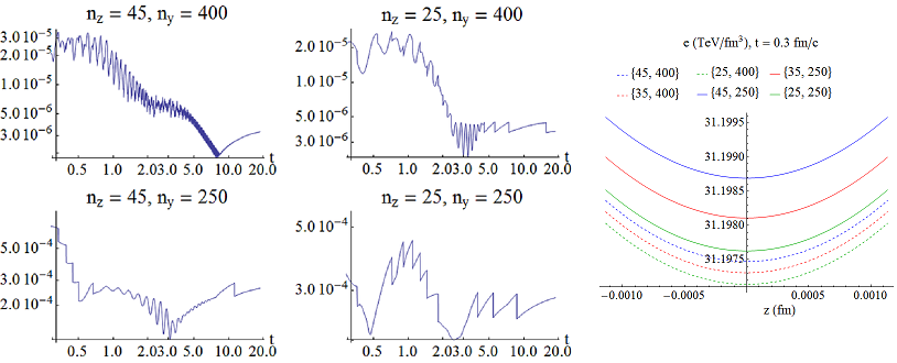
Figure 3.1: The maximum value of the constraint violation (last line of equation 5.2.2) as a function of time for various number of grid points ($n_{z}$ AdS direction, $n_{y}$ longitudinal direction). The constraint decreases when increasing $n_{y}$, but the $n_{z}$ dependence is weak (however, for narrower shocks one needs $n_{z}\approx 40$ for stable evolution). Note the discontinuities in the constraint violation, which are at points where the grid is changed to put the horizon at $r=1$, and/or smoothing is applied (see subsection 3.1.3). This plot is for a shock with $\mu w=0.75$, $\ell=0$ and $e_{reg}/e_{shock}=0.05$, with $e_{reg}$ the regulator energy density and $e_{shock}$ the peak of the ingoing shock energy density. These are the standard values of the package ‘shockwaves.nb’. The right plot compares the various solutions at the end of the evolution, around mid-rapidity. There is only a very small difference, mainly due to smoothing effects.

3.2.3 From full stopping to transparency [68]

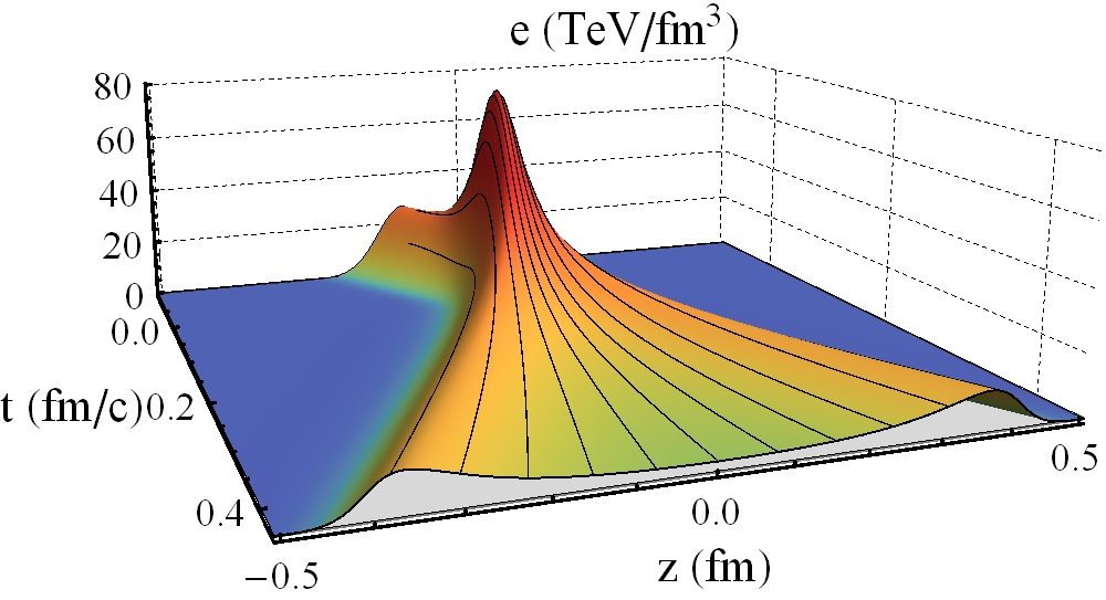
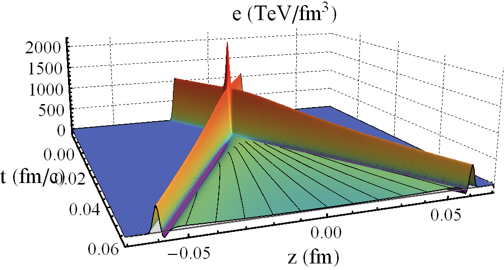
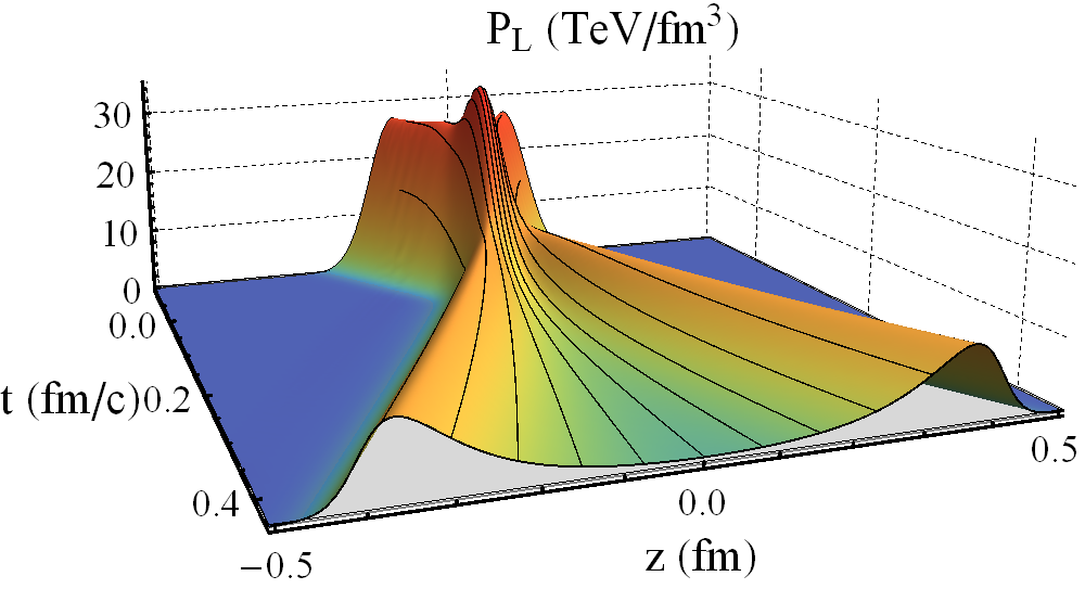
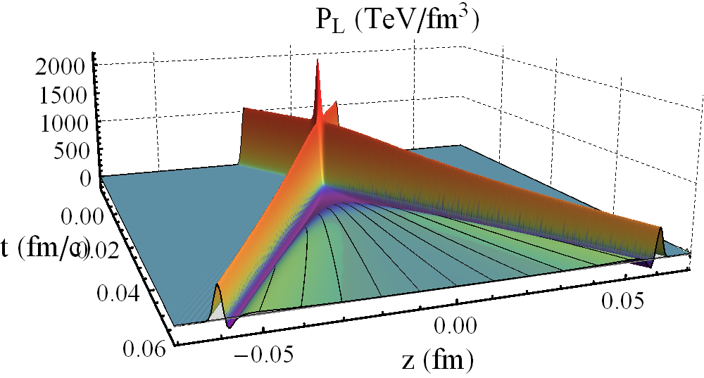
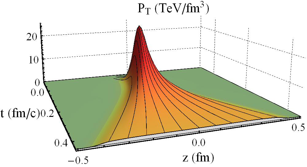
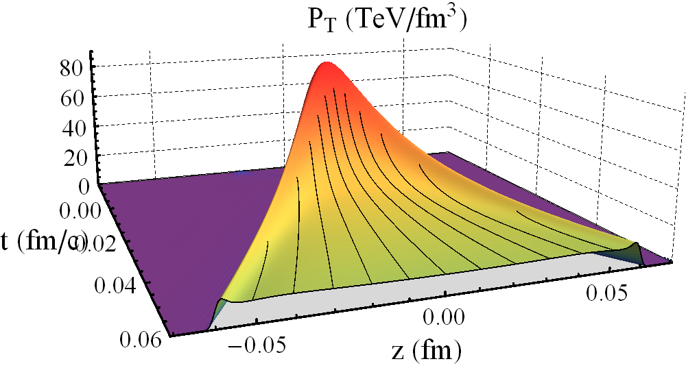
Figure 3.2: Energy density and pressures for collisions of thick (left row, $\mu w=1.9$ or $w=0.04$ fm) and thin (bottom row, $\mu w=0.05$ or $w=0.001$ fm) shocks as a function of time and longitudinal coordinate $z$. The grey planes lie at the origin of the vertical axes. As expected, the initial shocks only carry longitudinal pressure. Note that the transverse pressure for the narrow shock is surprisingly flat as a function of $z$, we will come back to this in figure 3.14.

An interesting cross-over occurs between what we call wide shocks (eqn. 3.2.1 with $\ell=0$ and $\mu w\gtrsim 0.5$) and thin shocks ($\mu w\lesssim 0.25$). These are represented in figure 3.2 by the energy densities and pressures of simulations with $\mu w=1.9$ (thick) and $\mu w=0.05$ (thin). It is clear that the thin shocks do not have time to thermalise during the collision, and hence they pass right through each other, forming a plasma only later on. On the other hand, for a bigger width the shocks can sufficiently thermalise already during the collision.

The thick shocks hence illustrate a full-stopping scenario. As the shocks start to interact the energy density gets compressed and ‘piles up’, comes to an almost complete stop, and subsequently explodes hydrodynamically. Indeed, at the time $t_{\text{max}}\simeq 0.020\,\text{fm}/c$ at which the energy density reaches its maximum in the top-left plot, the energy density profile is approximately a rescaled version of one of the incoming Gaussians, with about three times its height (see table 3.1) and 2/3 its width. At this time, $90\%$ of the energy is contained in a region of size $\Delta z\simeq 2.4w$ in which the flow velocity is everywhere $|v|\lesssim 0.1$. Similarly, the energy flux in this region is less than $10\%$ of the maximum incoming flux, as illustrated by figure 3.3(left). Importantly, it can also be checked that hydrodynamics is applicable, as can be seen in figure 3.4(left) and figure 3.5(left), where it is seen that hydrodynamics becomes applicable even before $t_{\text{max}}$.

The thin shocks illustrate a transparency scenario. In this case the shocks pass through each other and, although their shape gets altered, they keep moving at $v\simeq 1$, as seen in figure 3.3(right). The most dramatic modification in their shape is a region of negative $e$ and $P_{L}$ that trails right behind the receding shocks. While the negative $e$ only develops away from the centre of the collision, the negative $P_{L}$ is already present at $z=0$, as shown more clearly in the bottom-right plot of Fig. 3.5. These features are compatible with the general principles of Quantum Field Theory [80], since the ‘negative region’ is far from equilibrium and highly localised near a bigger region with positive energy and pressure. In the case of thin shocks, we see from figure 3.3(right) and figure 3.5(right) that there is a clear separation between non-hydrodynamic receding maxima and a plasma in between them that is described by hydrodynamics only at sufficiently late times. At sufficiently late times it is also visible from figure 3.2 that the receding maxima suffer significant attenuation. We therefore emphasize that our use of the term ‘transparency’ refers to time scales longer than $t_{\text{hyd}}$ but shorter than the attenuation time. Furthermore, this ‘transparency’ is not necessarily related to the similarly transparent model used in heavy-ion collisions. In particular, our model is not necessarily boost-invariant (see section 3.4) and all energy does end up in the plasma at late times, which suggests that these collisions are not necessarily transparent for baryon number density [81].

Several quantities of interest are given in table 3.1. We see that $t_{\text{max}}>0$ for thick shocks, whereas for thin shocks $t_{\text{max}}\simeq 0$, as it would be in the absence of interactions. Similarly, the maximum energy density $e_{\text{max}}$ is just the sum of the incoming energies $e_{\text{start}}$ for thin shocks, indicating that, unlike for thick shocks, there is no compression or piling up for thin shocks. The minimum energy density $e_{\text{min}}$ is negative for sufficiently thin shocks, as expected. The fact that $t_{\text{hyd}}<0$ is negative for thick shocks simply means that hydrodynamics becomes applicable even before the shocks fully overlap. The temperature at the moment of hydrodynamisation , $T_{\text{hyd}}$, is surprisingly constant. As in other models [39, 38], the product $t_{\text{hyd}}T_{\text{hyd}}$ is smaller than unity and fairly constant, which leads to hydrodynamisation times (significantly) shorter than 1 fm.

The anisotropy $P_{T}/P_{L}$ at the times where hydrodynamics is applicable increases as the width decreases, reaching values as large as $\sim 15$. It is remarkable that such strong anisotropies can be well described by first-order hydrodynamics. On the other hand hydrodynamics fails to describe the regions with negative pressure, as expected on thermodynamic grounds. It is therefore interesting that hydrodynamics really seems applicable ‘as fast as possible’.

   

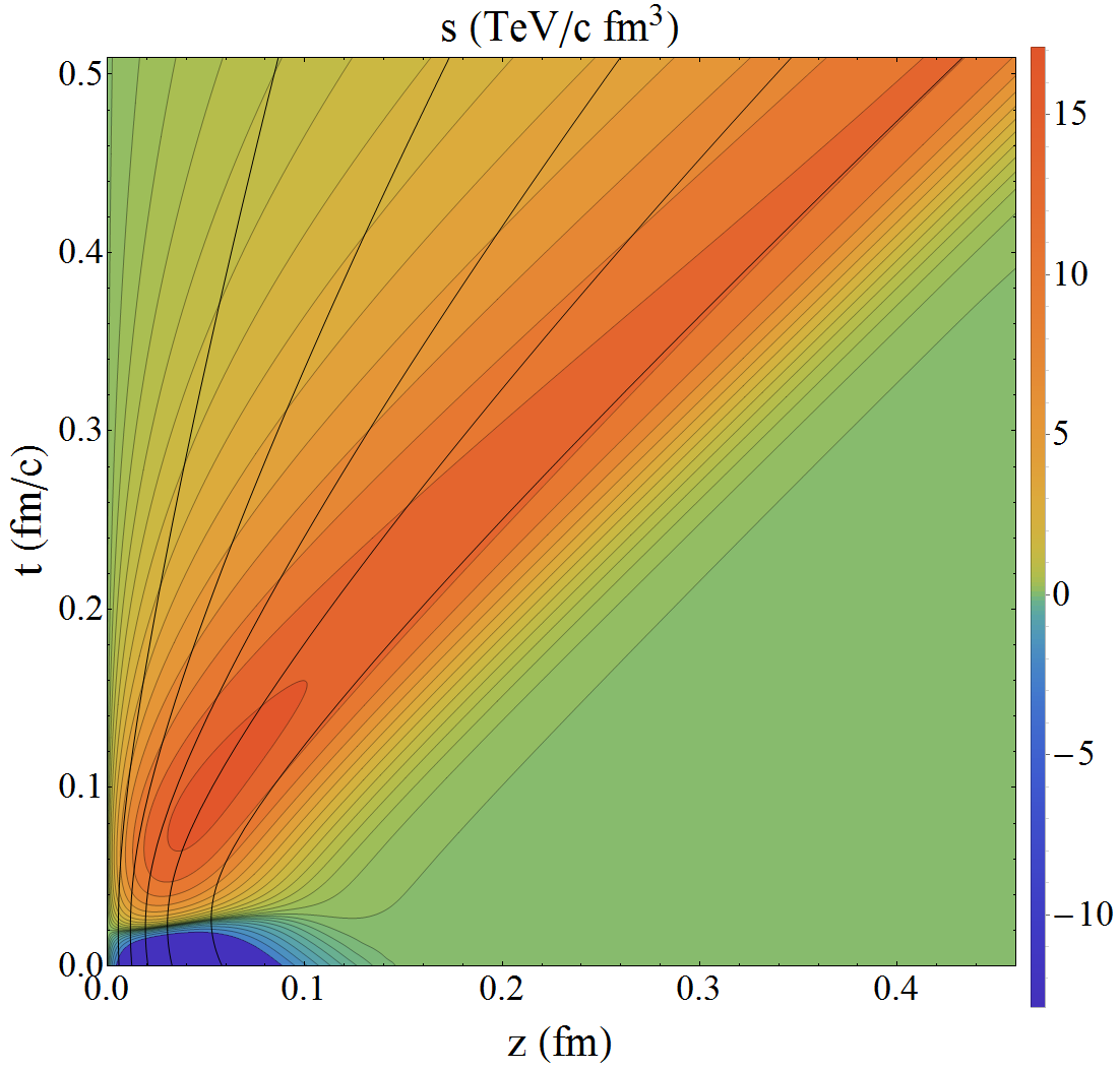
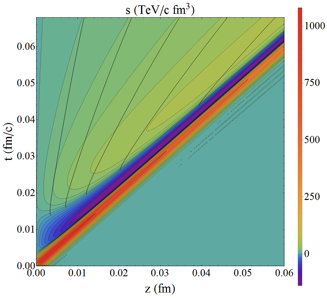
Figure 3.3: Energy flux for collisions of thick (left) and thin (right) shocks. The black lines are streamlines of the produced plasma.

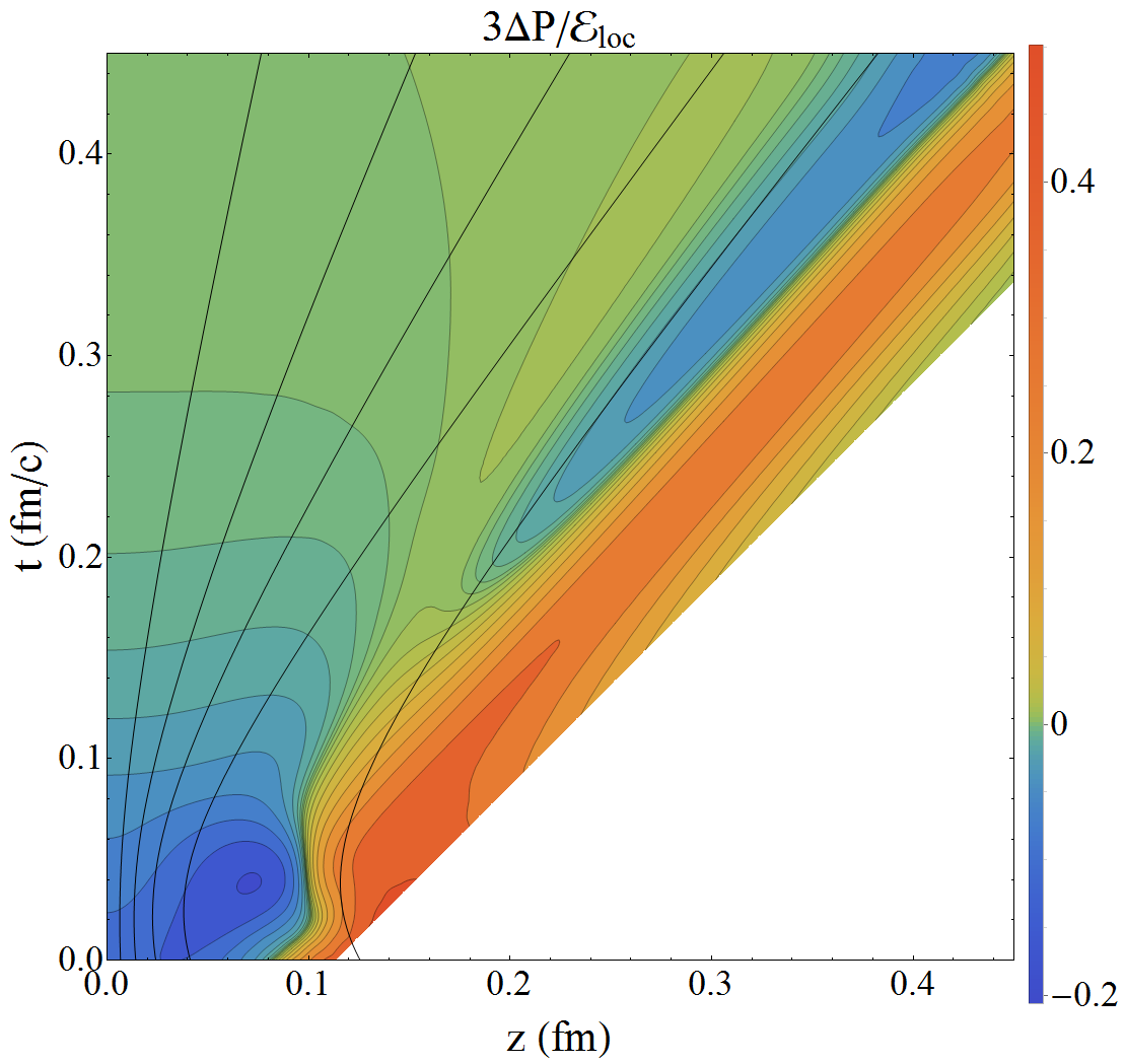
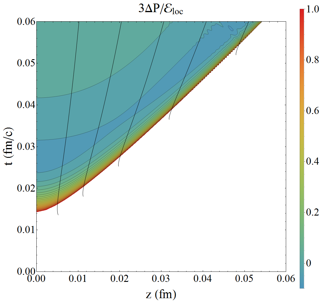
Figure 3.4: $3\Delta{\cal P}_{L}^{\textrm{loc}}/\mathcal{E}_{\text{loc}}$ for thick (left) and thin (right) shocks. The white areas indicate regions outside the lightcone or where hydrodynamics deviates by more than 100%. The black lines are again stream lines, whereby it can be seen that for narrow shocks a local restframe is only defined right before the region where hydrodynamics becomes applicable. As opposed to all other plots, these plots are evaluated using a single evolution without correcting for the regulator energy density, as this displays the transition to hydrodynamics most clearly.

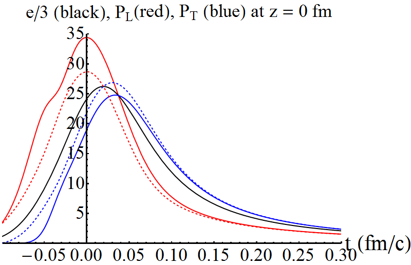
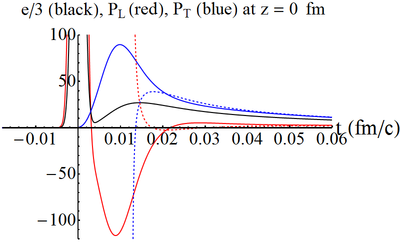
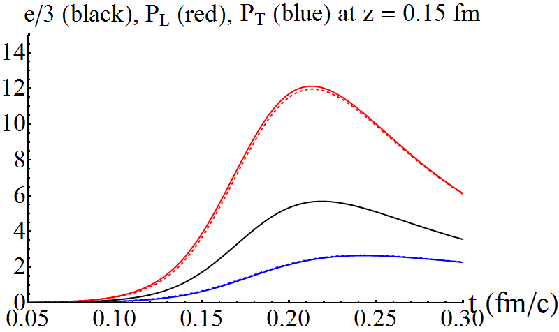
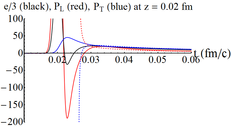
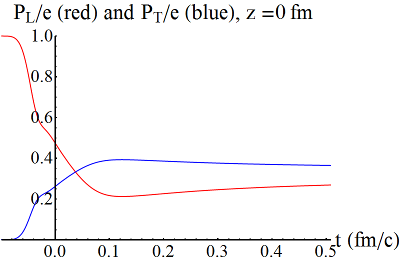
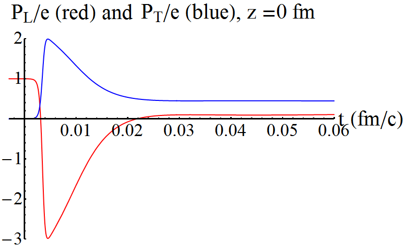
Figure 3.5: Energy density and pressures of wide (left) and narrow (right) shock wave collisions at the centre and off-centre (middle). The dashed lines indicate the prediction by first order hydrodynamics (eqn. 3.1.18). The last row plots the pressure over the energy density; the narrow shock ratios directly after the shock almost reach two and minus three, which agrees with analytic computations with delta-shocks [82].

The crossover can be heuristically understood on the gravity side (figure 3.6). Since each of the colliding shock waves is a normalisable solution in the bulk, the metric near the AdS boundary is a small deviation from AdS. Consequently, the gravitational evolution is linear near the boundary for some time $t_{\text{lin}}$. The deviation becomes of order one at $u\sim\mu^{-1}$, with $u$ the usual Fefferman-Graham holographic coordinate. At this depth gravity becomes strong and the evolution is non-linear. This non-linearity takes $t_{\text{lin}}\sim u\sim\mu^{-1}$ to propagate to the boundary. If $w\ll t_{\text{lin}}$, i.e. if $\mu w\ll 1$, there is a clear separation between the linear and the non-linear regimes. For thin shocks, this is illustrated by e.g. figure 3.5(left, top), where the energy density exhibits two maxima around $\mu t\sim 0$ and $\mu t\sim 1$. The former corresponds to the two shocks passing through each other; the latter corresponds to the arrival to the boundary of the non-linear pulse from the bulk. In this sense the pulse is responsible for the ‘creation’ of the plasma in between the thin receding shocks. Another clear manifestation is present near the light cone; the non-linear pulse takes longest to ‘catch up’ with the front of the shocks, which hence decay the latest, as is clear in figure 3.7. We note that in our simulations we always work with Gaussian shocks of finite size, so that the lightcone is also smoothed out; it is still an interesting question what happens in the true delta-limit [82].

In contrast, for thick shocks $\mu w\gg 1$, meaning that $t_{\text{lin}}\ll w$. In this case the pulse reaches the boundary before the shocks have passed through each other and essentially all the evolution is non-linear. In figure 3.6 this can be seen as a continuous thermalisation during the collision. The metric is therefore not never the sum of the incoming shocks, in contrast to the narrow shocks.

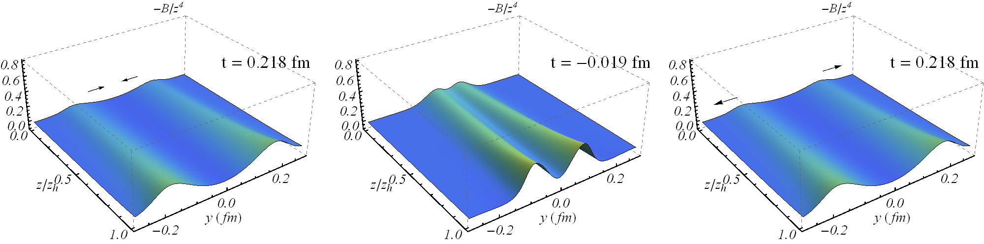
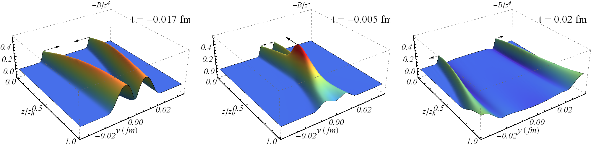
Figure 3.6: Here we illustrate the bulk dynamics by plotting $B/z^{4}$ between boundary and horizon at various moments for wide (top) and narrow (bottom) shocks. While $B$ is gauge dependent the figure still allows to understand the basic difference between both shocks. Firstly, one notices that in Eddington-Finkelstein coordinates the shocks collide earlier deep in the bulk. The non-linear dynamics there, however, arrives only at the boundary a time $\sim 1/2T$ after the shocks have collided. More importantly, it is apparent that the narrow shocks are a superposition for a larger time, as indicated by the ‘blob’ hitting the boundary. The wide shocks, on the other hand, thermalise continuously during the collision.

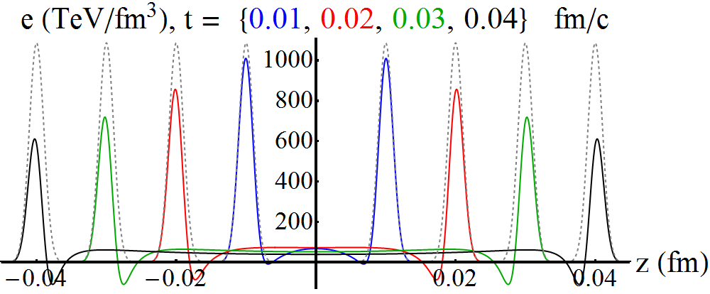
Figure 3.7: We plot snapshots of the energy density of figure 3.2 (right) at different times, including snapshots of the original shocks propagating without any interaction (dashed). The figure confirms our bulk interpretation that the shocks decay due to non-linear dynamics in the bulk, which in particular implies that the front of the shock decays latest, as it it takes bulk dynamics longest to ‘catch up’ with the front of the shock.

This analysis suggests that we have identified all the qualitatively different dynamical regimes. Presumably we have also considered values of $\mu w$ sufficiently representative of the asymptotic regimes $\mu w\gg 1$ and $\mu w\ll 1$. For thick shocks this is suggested by the fact that they come very close to a complete stop and subsequently evolve hydrodynamically. For thin shocks this is suggested by comparison of figure 3.5(bottom right) with [82]. This reference studied the delta-function limit $w\to 0$ with $\mu$ fixed and found that the pressure/energy ratios are $P_{L}/e=-3$ and $P_{T}/e=2$ at $t\to 0^{+}$. Figure 3.5(right) shows that these are also the extremum values attained by our thin shocks.

$w$(am)	$\mu w$	$t_{\text{max}}$(am/c)	$\frac{{\textstyle e_{\max}}}{{\textstyle e_{\text{start}}}}$	$\frac{{\textstyle e_{\text{min}}}}{{\textstyle e_{\text{start}}}}$	$t_{\text{hyd}}$(am/c)	$T_{\text{hyd}}$(GeV)	$t_{\text{hyd}}T_{\text{hyd}}$
43.0	1.89	19.4	2.9	0.	-2	2.6	-0.02
17.0	0.75	3.5	2.3	0.	34	2.6	0.45
6.7	0.30	0.6	2.0	0.	23	2.7	0.32
2.7	0.12	0	2.0	0.	20	2.6	0.27
1.8	0.08	0	2.0	-0.01	20	2.6	0.27
1.1	0.05	0	2.0	-0.1	20	2.6	0.26

Table 3.1: Numerical values of several quantities of interest for single shocks ($\ell=0$).

3.3 Longitudinal coherence

It is an interesting question if the plasma created in the collisions of section 3.2 depends on the longitudinal structure of the colliding objects, which was previously restricted to be a Gaussian. In heavy-ion collisions this structure would be more complicated, but perhaps even more interesting are recent proton-lead collisions. These are inherently a-symmetric, where in the centre-of-mass frame the energy density of the proton would be much more concentrated than the energy density of the nucleus.

To study the dependence on the longitudinal structure figure 3.8 shows the energy density for the two collisions in the second row of Table 3.2: a coherent collision with (eqn. 3.2.1with $\ell=8w$ and $\mu w=0.05$) (left) and an incoherent collision with $\ell=32w$ and $\mu w=0.05$ (right). These are shocks composed of two Gaussian ‘thin’ constituents (as in subsection 3.2.3) which are separated by $\mu\ell=8\mu w=0.4$ (left) and $\mu\ell=32\mu w=1.8$ (right). As expected from subsection 3.2.3, the thin constituents pass through each other virtually undisturbed and then start to attenuate. Close to the light-cone, both figures show the initial shock profiles after the collision, indicating that in both cases the high-rapidity region is sensitive to the initial structure of the shocks.

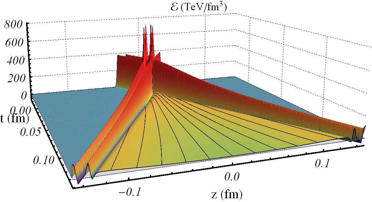
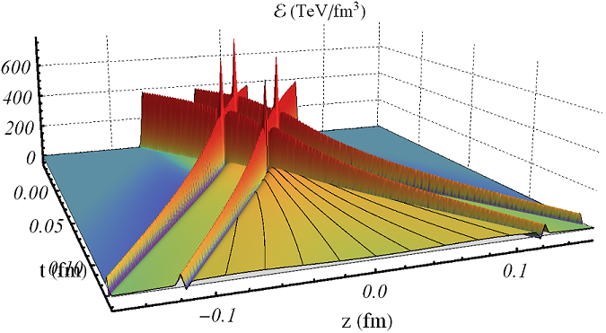
Figure 3.8: Energy density of two collisions composed of narrow shocks with separation $\ell=8w$ (left) and $\ell=32w$ (right), with $w=0.05/\mu=0.001$ fm. The black lines are streamlines of the produced plasma.

In contrast, the mid-rapidity region of figure 3.8 (left) keeps no memory of the initial structure of the shocks. This is illustrated in figure 3.9 (left), which shows snapshots of the energy density at a fixed time after hydrodynamisation, $t=0.05$ fm, for the several collisions with different initial shock structures but with the same total energy listed in the left part of Table 3.2. We see that the energy density around mid-rapidity for the single-double collision of 3.8 (left) is identical to that for a single-single or a double-double collision with constituents of the same width, and for a single-single collision with twice-as-thick constituents. In all these cases the hydrodynamisation time and the hydrodynamisation temperature are independent of the initial structure of the shocks. For single shocks this is consistent with section 3.2, where it was found that the hydrodynamisation properties of the plasma are independent of the widths of the initial shocks provided these satisfy $\mu w\lesssim 0.2$.

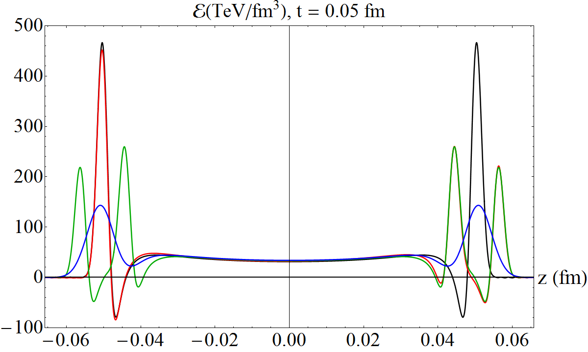
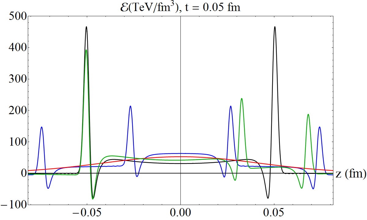
Figure 3.9: Energy density at $t=0.05$ fm for different shock collisions characterised by the parameters displayed in Table 3.2.

Table 3.2: Parameters of the shocks displayed in figure 3.9. The 8/0 indicates an asymmetric collision with different $\ell$ for left and right moving shocks.

	Left					Right
	$\mu w$	$\ell/w$	$t_{\text{hyd}}$	$T_{\text{hyd}}/\mu$	$\ell T_{\text{hyd}}$	$\mu w$	$\ell/w$	$\mu t_{\text{hyd}}$	$T_{\text{hyd}}/\mu$	$\ell T_{\text{hyd}}$
Black	0.05	0	0.88	0.30	0.05	0.05	0	0.88	0.30	0.05
Red	0.05	8/0	0.88	0.30	0.12	1.9	0	0.95	0.31	0.36
Green	0.05	8	0.88	0.30	0.12	0.05	32/0	1.20	0.33	0.48
Blue	0.10	0	0.88	0.30	0.1	0.05	32	-0.08	0.30	1.9

Figure 3.9(right) shows analogous snapshots for the collisions listed on the right part of table 3.2, which again have the same total energy but differ in the initial structure of the shocks. One of the curves is the same single-single collision of thin shocks from figure 3.9 (left), which is included for comparison. The other three curves all have $\ell>0.26/T_{\text{hyd}}$ and they illustrate the incoherent regime, namely the fact that the energy density around mid-rapidity, as well as the hydrodynamisation time and the hydrodynamisation temperature, are sensitive to the initial structure of the shocks. Note that the different hydrodynamisation temperatures would translate into about a 30% difference in the energy density at mid-rapidity (which scales roughly as $T_{\text{hyd}}^{4}$) even if each of these curves were plotted at its corresponding hydrodynamisation time.

From the gauge theory viewpoint, these results imply that the smallest longitudinal structure that the fields in the mid-rapidity region can resolve is set by the inverse temperature at hydrodynamisation, which in the coherent regime is $T_{\text{hyd}}=0.3\mu$. Clearly, the plasma will be sensitive to the structure of the initial shocks if their characteristic size, $\ell_{\text{char}}$, is larger than the formation time of the hydrodynamised plasma, $t_{\text{hyd}}$. By inspection of table 3.2 we see that the transition between the coherent and the incoherent regimes takes place at a scale $\ell_{\text{coh}}$ such that $0.12<\ell_{\text{coh}}T_{\text{hyd}}<0.36$. Since this transition is smooth, $\ell_{\text{coh}}$ is not sharply defined. Motivated by the considerations above, we therefore choose to define it as the hydrodynamisation time for single-single collisions of thin shocks, which yields $\ell_{\text{coh}}=0.26/T_{\text{hyd}}$.

This picture is supported by the gravitational description. In figure 3.10 we show the entropy density from the apparent horizon formed in the two collisions displayed in figure 3.8. Although this quantity depends on the slicing of the space-time, close to equilibrium it provides a lower bound for the entropy density [83]. According to the gauge/gravity duality, the horizon encodes the physics at the thermal scale. Heuristically, one may say that figure 3.10 provides an effective picture of figure 3.8 in which all length scales shorter than the thermal scale have been integrated out. It is therefore suggestive that in figure 3.10 (left) there is no trace of the microscopic structure of the shocks even at the time $t=0$ of the collision. In contrast, for the further-separated colliding shock constituents of figure 3.8 (right), the corresponding apparent horizon in figure 3.10 (right) reflects the initial configuration, albeit with a significant smoothing due to the integration of scales.

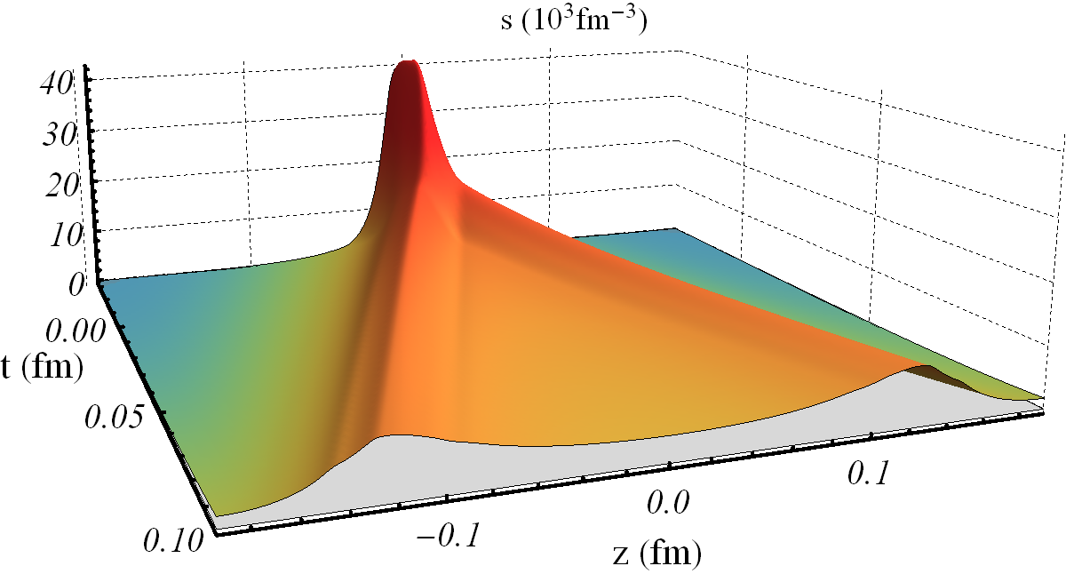
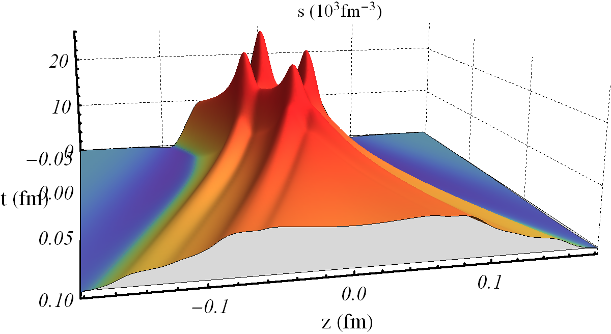
Figure 3.10: Entropy density $s$ found by computing the volume element on the apparent horizons formed in the two collisions depicted in figure 3.8. Note that the entropy is only defined near equilibrium, so that outside this region $s$ should be interpreted as a lower bound on the entropy which is going to be produced.

3.3.1 Consequences for HIC

Since longitudinal coherence only depends on the inability of the horizon to resolve sub-thermal length scales, we expect this coherence to occur in holographic high-energy collisions more general than the simple model considered here. These may include collisions of shocks with profiles more general than eqn. 3.2.1 and collisions with non-trivial transverse dynamics, at least if the transverse expansion rate is slower than the longitudinal one. In the following we take this as an assumption and explore interesting consequences for high-multiplicity (p/d)+A collisions. Furthermore, we consider the limits in which the physics of bulk-particle production is assumed to be exclusively strongly or weakly coupled, the hope being that these limits bracket the production dynamics at the energies of present colliders.

In the strong coupling limit our results, together with the large Lorentz contraction of the colliding projectiles at RHIC and LHC, suggest that most of the participating nucleons act coherently in the formation of the plasma. As a consequence, the momentum rapidity of the plasma’s c.o.m., $y_{\text{plasma}}$, should coincide with the momentum rapidity of the c.o.m. of all the participating nucleons, $y_{\text{part}}$. Since the local energy density at fixed proper time is maximal at $y_{\text{plasma}}$ [68, 45], the maximum in the rapidity distribution of particles, $y_{\text{max}}$, also coincides with $y_{\text{part}}$. For a generic collision with $N_{\text{A}}$ ($N_{\text{B}}$) right-moving (left-moving) participating nucleons moving at rapidity $y_{\text{A}}$ ($y_{\text{B}}$), we have that $y_{\text{part}}=\tfrac{1}{2}\,\log(N_{\text{A}}/N_{\text{B}})+y_{\text{NN}}$, where $y_{\text{NN}}=\tfrac{1}{2}(y_{\text{A}}+y_{\text{B}})$ is the rapidity of the nucleon-nucleon c.o.m. As a consequence, event-by-event fluctuations in the number of participating nucleons in A+A collisions lead to fluctuations in $y_{\text{max}}$ according to $y_{\text{part}}$, as was also studied in [84]. Similarly, in p(d)+A collisions $y_{\text{max}}$ shifts to the A side due to the asymmetric collision geometry. Taking $N_{A}=15-30$ as representative values for central p(d)+A collisions at the LHC (RHIC) we find $y_{\text{max}}=0.9\,(1.3)-1.2\,(1.7)$. An additional result of the strong-coupling model is that the plasma is $y$-reflection-symmetric around $y_{\text{plasma}}$. Interestingly, particle production in d+A collisions at RHIC [85] seems consistent with both of these features, as already noted in [86].

At weak coupling we may determine $y_{\text{max}}$ via perturbative QCD. For nuclei moving at large rapidities, $\left|y_{\text{A}}-y_{\text{B}}\right|\gg 1$, this can be estimated by equating the squared saturation scales of both colliding objects [87], $Q_{s}^{2}(N_{\text{A}},y_{\text{max}})=Q_{s}^{2}(N_{\text{B}},y_{\text{max}})$. Far from its own rapidity $y_{\text{C}}$, the saturation scale of a nucleus with $N_{\text{C}}$ participating nucleons evolves as $Q_{s}^{2}(N_{\text{C}},y)\sim N_{\text{C}}\exp\left(\bar{\lambda}\left|y-y_{\text{C}}\right|\right)$ [88, 89]. The coupling-dependent exponent $\bar{\lambda}$ can be extracted from fits to HERA data within the saturation framework [90] and is given by $\bar{\lambda}\simeq 0.25$ [88, 89], reflecting the fact that in perturbative QCD the fraction of energy available for particle production decreases with energy. Substituting in the equation for $y_{\text{max}}$ we find $y_{\text{max}}=\frac{1}{2\bar{\lambda}}\,\log(N_{\text{A}}/N_{\text{B}})+y_{\text{NN}}$.

Another interesting consequence applies to off-central nucleus-nucleus collisions. There the rapidity dependence of the direct flow $v_{1}$ depends crucially on the longitudinal deposition of the energy [91]. In this work the ‘firestreak model’ shifts rapidity to the centre-of-mass just like our proposal above. Quite surprisingly reference [91] found that this does not produce the correct direct flow as a function of rapidity. Interestingly, if one replaces their boost-invariant rapidity profile with the rapidity profile of section 3.4 the direct flow seems to be closer to the experimental value (see figure 3.11).

Lastly, our coherent picture will mean that at a fixed position in the transverse plane the correlations in the longitudinal direction will be basically constant over the complete range. This is because the plasma will only be sensitive to the total energy per transverse area, whereby more energy will just increase the energy density over the total longitudinal range. Of course, there will still be thermal fluctuations ($1/N_{c}$ supressed in our set-up), such as interestingly studied in [92]. This therefore means that we expect fluctuations in the longitudinal direction to be solely due to thermal fluctuation, as opposed to transverse fluctuations, which originate both from initial state fluctuations and thermal fluctuations. To measure thermal transport coefficients it can therefore be beneficial to focus on longitudinal dynamics.

We thus conclude that longitudinal coherence has consequences for off-central nucleus-nucleus collisions and for proton-nucleus collisions, whereby strong- and weak-coupling predictions are considerably different. Especially the value for $y_{\text{max}}$ in p+A collisions differs by about a factor of four. This makes the possible experimental extraction of $y_{\text{max}}$ from RHIC [93] or LHC [94] d/p+A data extremely interesting, since the result may help constrain the mechanism of bulk-matter production.

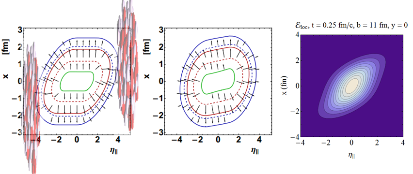
Figure 3.11: The figure on the left (adapted from [91]) represents constant pressure contours for initial conditions for an off-central collision computed by assuming coherence and a plateau in rapidity. This initial condition turns out not to produce the correct direct flow $v_{1}(\mbox{$\eta$)}$, whereas a phenomenologically inspired tilt (middle figure, from [91]) does produce the correct $v_{1}(\mbox{$\eta$)}$. On the other hand, if one uses a Gaussian rapidity distribution with width 0.95 (see section 3.4) the initial condition looks similar to the tilted one, with using coherence (right). It is interesting that planar shock waves give such interesting consequences for these off-central collisions.

3.4 Rapidity profile: Bjorken vs Landau?

In heavy-ion collisions there are two interesting models to describe the initial longitudinal dynamics. The first one is described by Landau [95] in 1953, where he assumes the two nuclei to be completely equilibrated and at rest at the moment they completely overlap. Due to all the energy being concentrated in an extremely small volume, this model will lead to a violent, but hydrodynamic, explosion afterwards. An impressive success of the Landau model is its prediction that the total number of particles scales as $s_{NN}^{1/4}$, which holds experimentally for a very large range in collision energies $\sqrt{s_{NN}}$ [96, 97, 98], albeit being violated at LHC [99] (see also subsection 3.4.2).

Importantly, while the Landau model seems to reproduce the total particle number (see however subsection 3.4.2), it is not generally believed to be an accurate description of heavy-ion collisions. Partly, this is because at such high energies the coupling of QCD is generally not assumed to be strong enough to cause the needed stopping. More importantly, it is experimentally found that the conserved baryon number (the number of protons minus antiprotons) ends up at high rapidities [81], which may be unnatural in the Landau model. In the current AdS model there is no such conserved charge, but we plan to report on this in the near future.

The second model was developed much later, in a famous paper by Bjorken [100]. Building on previous intuition [101, 102] he assumed interactions to be sufficiently weak such that the nuclei could pass through each other, virtually unperturbed. In the middle a plasma would form, which would be invariant under boosts, or equivalently shifts in rapidity. Here, proper time $\tau$ and rapidity $y$ are defined by $t=\tau\cosh y$ and $z=\tau\sinh y$. Of course it is not possible to have a boost-invariant plasma for all rapidities (it would require infinite energy), but one may imagine that the range of approximate boost-invariance will grow with growing collision energy.

The basic assumptions of these two models cannot be derived from (strongly coupled) QCD. It is therefore of great interest to see how our results, at infinite coupling, fit into these two models. Indeed, our full-stopping scenario is in close similarity with the Landau model, as was already clear in [39]. Perhaps the only difference is that we find a very specific energy ($\mu w=0.75$, also used in [39]) to realise the Landau model, whereas the Landau model is supposed to be correct for a wide range of energies. At lower energies, there is a significant ‘piling up’ of energy. This will reduce the scaling $s_{NN}^{1/4}$ somewhat, but probably too little to be easily detectable experimentally.

At high energies we find a transparent regime, showing that infinite coupling does not necessarily lead to full stopping and is compatible with receding shocks moving at the speed of light. Indeed, a simple field theory scaling argument shows that this is inevitable. In the Landau model the inverse temperature of the equilibrated plasma scales as $e^{-1/4}\sim(\mu^{3}/w)^{-1/4}\sim\gamma^{-1/2}$, and can be thought, both thermodynamically and quantum mechanically, as the minimum time scale or distance required to interact. The width, however, scales as $w\sim\gamma^{-1}$, such that it is easy to see that for large enough $\gamma$ the width is smaller than the minimum time to interact, and hence the shocks necessarily pass through each other: they do not have time to thermalise.

The plasma formed by the narrow shocks, however, does not obey the boost-invariance of the Bjorken model. This is most easily seen in figure 3.12, where we have changed to proper-time and spacetime-rapidity coordinates. The ‘tubes’ at late times show that the local energy density at mid-rapidity is not rapidity-independent but has an approximately Gaussian profile of width about 0.95 in the transparent regime.

It is sensible to ask how figure 3.12 would look like in limit of infinite collision energy. This can be answered by realising that longitudinal coherence (section 3.3) shows a plasma at mid-rapidity which is independent of $\mu w$, provided $\mu w$ is small enough. We can therefore say that figure 3.12(right) is already very close to the delta-limit, or infinite energy limit, where $\mu w=0$. We therefore believe to have arrived at a universal high energy rapidity profile for conformal theories at infinite coupling, which is notably different from the Bjorken model above.

  

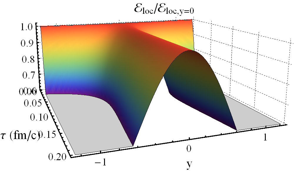
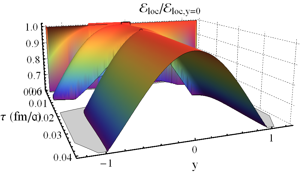
Figure 3.12: Energy density in the local rest frame around mid-rapidity as a function of spacetime rapidity $y$ and proper time $\tau$ for thick (left) and thin (right) shocks (the same shocks as figure 3.2). In the right case we have excluded from the plot the region in which the local rest frame is not defined because $2|s|>|e+P_{L}|$.

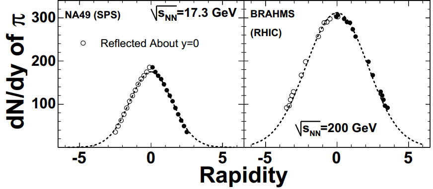
Figure 3.13: Particle multiplicities of $\pi^{-}$ and $\pi^{+}$ particles at $\sqrt{s_{NN}}=17.3$ GeV (SPS, [103]) and $\sqrt{s_{NN}}=200$ GeV (RHIC, [104]). The dashed lines are fitted Gaussians of width $1.42\pm 0.02\,\text{(stat)}$ and $2.25\pm 0.02\,\text{(stat)}$ respectively, the figure is taken from [105, 106]. It can be seen that the Gaussians describe the distribution well, which was our main motivation when comparing figure 3.12 with a Gaussian. It should be kept in mind, however, that these experimental data represent the final rapidity distribution, and hence do not necessarily agree with the initial distribution, such as we try to compute. Also, measuring rapidity distributions necessitates measuring particle masses, which at LHC is unfortunately not possible over the full range of rapidities.

3.4.1 Local energy density in real time

  

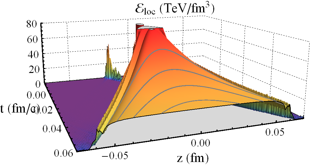
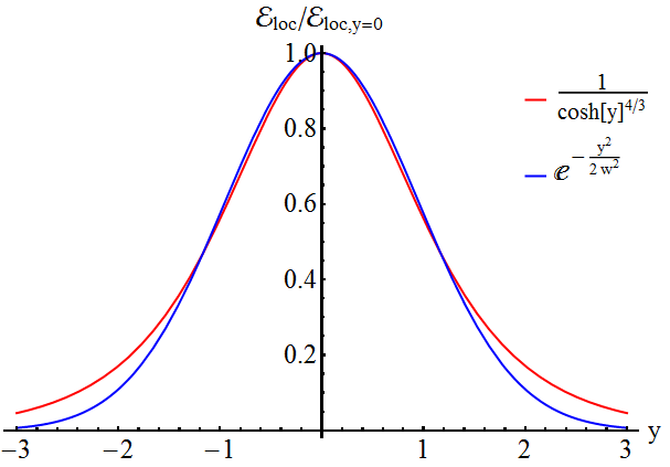
Figure 3.14: Energy density in the local rest frame as a function time and space for thin shocks with constant proper time curve (grey). The curve is remarkably flat shortly after the applicability of hydrodynamics It is an open problem to understand this flatness, but it can be used to estimate the rapidity profile plotted in figure 3.12 being $\cosh(y)^{-4/3}$. At the right this shape is compared to a Gaussian of width 0.95, and they fit remarkably well in the region we can compare with our theoretical computation (figure3.12) or even with experimental data (figure3.13). Current simulations for LHC collisions would start with a completely flat profile for $y\in(-5,\,5)$ [107].

Interestingly, the rapidity shape described above may have a more natural interpretation in real space, instead of rapidity space. When plotting the local energy density as a function of time and space for narrow shocks (figure 3.14, left), one notices that shortly after the applicability of hydrodynamics (at around 0.02 fm) the local energy density is remarkably flat as a function $z$ at fixed $t$ (real time!). This could already be noticed by looking at the transverse pressure (figure 3.2 lower right), which is already in the local rest frame. We stress that the constancy of $e_{\text{loc}}$ should come as a surprise; in fact, we could not think of an argument independent of our numerical simulation. In particular, a boost-invariant $e_{\text{loc}}$ would look very differently, being constant along the grey lines in figure 3.14 or flat in figure 3.12. There is no real translation symmetry in $z$ either, as the velocity profile approximates the expected $z/t$ well. Note also that $e_{\text{loc}}$ will not remain constant at later times; the hydrodynamic expansion will widen the rapidity distribution, which will change $e_{\text{loc}}$. This, however, is just due to hydrodynamics and therefore of lesser interest in our context of thermalisation.

With this extra understanding it is then only natural that at constant proper time $\tau$ (grey lines in figure 3.14) the energy density decreases with rapidity $y$. We can write $e_{\text{loc}}(t,\,z)=f(t)$, where $f(t)$ will decrease due to the expansion and longitudinal pressure of the plasma. In the regime plotted this can be fairly well approximated as $f(t)\sim t^{-4/3}$, which is also the late time boost-invariant result. As a function of proper time this gives

$$e_{\text{loc}}\sim(\tau\,\cosh(y))^{-4/3}.$$ (3.4.1)

Comparing this rapidity shape with the Gaussian conjectured above leads to very similar curves until $\mathcal{E}_{\text{loc}}/\mathcal{E}_{\text{loc,y=0}}\approx 0.3$ (figure 3.14, right), below which it is difficult to make either theoretical calculations (figure 3.12) or experimental measurements (figure 3.13). So perhaps the rapidity profile is more similar to $\cosh(y)^{-4/3}$ instead of a Gaussian. This would also provide a natural explanation why the Gaussian has width 0.95.

3.4.2 Multiplicities and a comparison with experiments

  

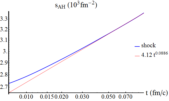
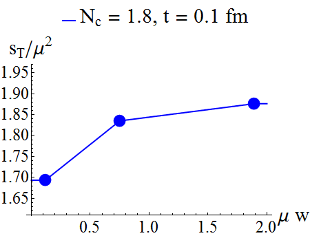
Figure 3.15: Using figure 3.10 we can obtain the total entropy per transverse area for thin shocks as a function of time. We find that most entropy is already produced before $t=0$, and that the late-time increase is well described by a slow power of $t$. On the right we evaluated this total entropy for several shock simulations at $t=0.1$ fm, showing a mild dependence on the width.

Given that the computations above suggest a universal rapidity profile (figure 3.12) in the high energy limit, it is interesting to ask if this kind of shape may be realised in real heavy-ion collisions. It is challenging to compare directly with experiments, firstly because the plasma evolution can significantly change the profile, and secondly it is only possible to measure the pseudo-rapidity (related to the angle of flight $p_{z}/|p|$), which can only be converted to real rapidity (related to $p_{z}/E$) if the particle mass is known.

An indication that a Gaussian-like initial profile can be realistic comes from RHIC, where it is possible to convert to rapidity and an approximately Gaussian shape was found (see figure 3.13). The width of this Gaussian grows with energy, but it is unclear how much of this growth is due to evolution or due to the initial profile.

To make such an estimate we can compute the initial entropy, which is approximately conserved during the evolution if the viscosity is small enough. This entropy $S$ directly translates into the total number of charged particles produced: $N_{charged}=S/7.5$ [108, 109, 74]. While the shock waves only simulate collisions which are homogeneous in the transverse plane, it is not unreasonable to assume that the entropy density in the first moments (where the longitudinal size is much smaller than the transverse size) does not depend much on transverse gradients. If most of the fluid is then well described by hydrodynamics, one can obtain a good estimate of the total entropy of the collision debris. Figure 3.15 indicates that this is indeed the case.

  

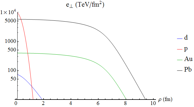
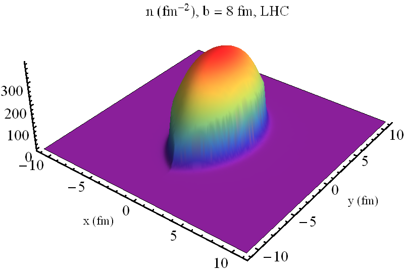
Figure 3.16: Using the total entropy per transverse area as a function of the energy scale $\mu$ and the width $w$ (figure 3.15) we can use this to compute the total entropy for various transverse energy densities (left, values from [76]). As an example we plot the multiplicity per transverse area for an LHC lead-lead collision (right).

The only other input needed is the centre-of-mass energy density as a function of the transverse plane, which we take from an optical Glauber model (eqn. 3.2.2). We then integrate the total entropy over the transverse plane, depending on the impact parameter $b$, to get an estimate of the total entropy and multiplicity. Figure 3.17 plots the resulting multiplicities for gold-gold, deuteron-gold, lead-lead and proton-lead collisions, starting with the energy profiles of figure 3.16.

Even at RHIC the multiplicity is higher than the experimental result, which contrasts slightly with previous claims that the Landau model could give the right particle multiplicity [97, 74]. This is largely due to a significant entropy production by viscous effects, which were previously neglected. On the other hand we should note that we did not take into account that a real nucleus is shaped irregularly, and that therefore some nucleons will not collide, which will reduce the multiplicity by perhaps $10-15\%$. For deuteron collisions the fit is also worse, but it should be kept in mind that the uncertainty for the deuteron shape is considerable.

Nevertheless, the agreement is much worse at LHC (consistent with previous results [74, 110, 111, 112]). As the total energy of a collision is conserved this means that real central collisions have only part of their energy deposited in the plasma (unlike our results), or the energy per particle in real collisions is considerably higher. As our initial conditions are unlikely to produce less radial flow this energy per particle would most likely be in the longitudinal direction. This would imply that real collisions have a broader rapidity profile than the profile found in section 3.4, which can perhaps be thought of as an effect of the infinite coupling approximation.

Although the mismatch between experimental data might seem worrisome, we do not think this is the case. Firstly, it is reassuring that the qualitative trends in figure 3.17 are well respected. Secondly, it is natural to expect that taking the infinite coupling limit produces too much stopping. Lastly, we stress that our model basically has no free parameters at all. Conventional models usually have the normalisation of the initial energy density, the coupling constant or other parameters which are more or less free, or fitted to related experiments. In the AdS/CFT model the only real freedom is the number of colours $N_{c}$, which has little effect on the total multiplicity. In this light the presented mismatch is not surprising, but an opportunity to improve the model by including weak-coupling effects in systematic or less systematic ways, which is partly the topic of the next chapter.

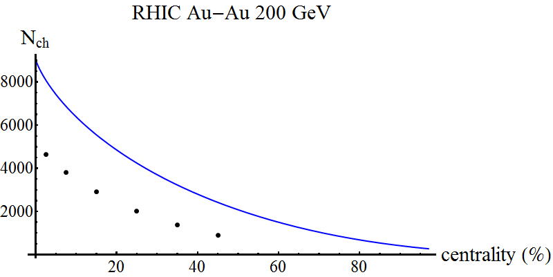
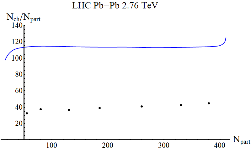
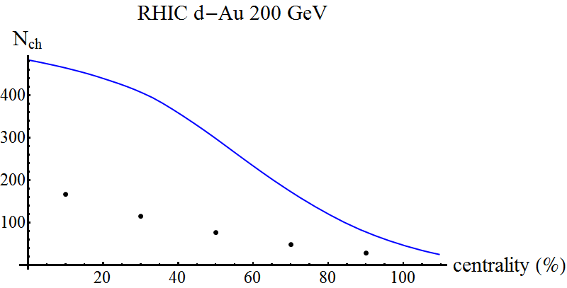
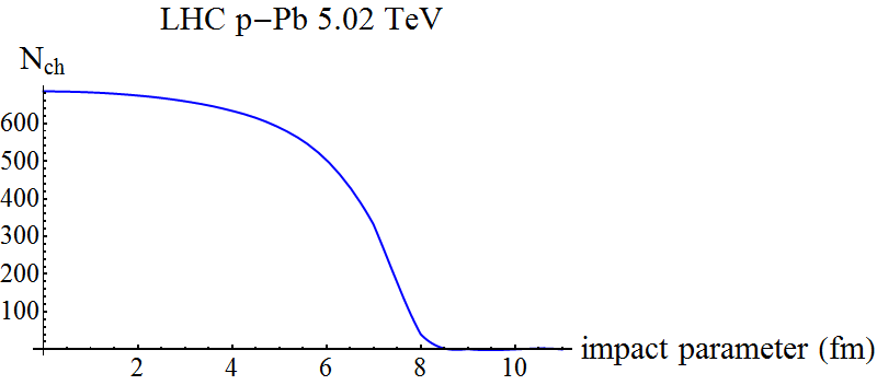
Figure 3.17: We plot the total number of charged particles for the models of figure 3.16. The centrality is computed using formula 1.1.1, the number of participants by integrating the energy in the region where the energy density of the left and right moving shock differs by less than a factor of 15. The mismatch at RHIC is slightly surprising, but can be traced back to mainly viscous effects. The mismatch at LHC confirms previous work [74, 111, 112], and is generally considered to be due to using infinite coupling. Nevertheless, the qualitative trends are well reproduced and furthermore we would like to stress that our simple model does not have any free parameters and one can therefore optimistically say that the result is rather close to the experimental results.

Chapter 4 Thermalisation with radial flow

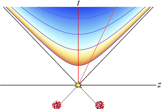
Figure 4.1: A simple and often used model of a heavy-ion collision was proposed by Bjorken [100], where he assumed that a heavy-ion collision is approximately boost-invariant, at least near $z=0$. This means that all physics only depends on proper time $\tau=\sqrt{t^{2}-z^{2}}$, and hence that all physics experienced by observers, such as a temperature field illustrated here, is independent of its frame. The two red lines would illustrate two such frames, which indeed has equal temperatures at equal$\tau$.

Most AdS/CFT studies, including the previous chapters, have completely neglected dynamics of heavy-ion collisions in the transverse plane. This is unfortunate, since the build-up of momentum in the transverse plane is directly related to experimentally measurable quantities. Including transverse dynamics in the shock wave collisions of chapter 3 is possible, but numerically more involved. Here instead, we will approximate the longitudinal dynamics as boost-invariant (see figure 4.1), as is usually done in studies of heavy-ion collisions. Furthermore we assume rotational symmetry, restricting ourselves to head-on collisions, thereby keeping the numerical code effectively 2+1 dimensional.

Firstly, we present two simple initial conditions; the first starts with a blob of energy with a diameter of approximately 14 fm in vacuum, whereas the second has a blob of about 1 fm in a bath of half the peak energy density. These initial states can model the overall thermalisation of a central collision and the evolution of an initial fluctuation in such a collision. Fluctuations are caused by the random distribution of protons and neutrons in nuclei will lead to large fluctuations in the (local) distribution of energy, which can is measured [114, 115] and interesting to study [116, 117, 118, 1, 107]. For the bulk metric we started with vacuum AdS, but adapted the near-boundary coefficients for the energy density and the pressures according to the Glauber model.

Thereafter a more ambitious project is presented, where the initial data is inspired from a small-time expansion of shock wave collisions [119]. The resulting stress-tensor is then evolved using a state-of-the-art hydrodynamics solver [120], including a final hadronic cascade code [121]. This allows a direct comparison with experimental data, which fits surprisingly well. We will explicitly show the main advantage of this AdS/CFT approach, being the dynamical transition from far-from-equilibrium to hydrodynamics, which in other models usually has to be assumed.

4.1 The holographic set-up with two examples

As our coordinates in the field theory it is natural to use proper time $\tau$ and rapidity $y$, defined by $t=\tau\cosh y$ and $z=\tau\sinh y$, and angular coordinates $\rho$ and $\theta$ in the transverse plane. The assumptions of boost-invariance and rotational symmetry then imply that all functions are independent of $y$ and $\theta$. In these coordinates the flat metric of the field theory reads

$$ds_{B}^{2}=-d\tau^{2}+d\rho^{2}+\rho^{2}d\theta^{2}+\tau^{2}dy^{2}.$$ (4.1.1)

Given these symmetries and using generalized Eddington-Finkelstein coordinates, we can write the dual AdS metric 2.1.1 as

$$ds^{2}=d\tau(-Ad\tau+2dr+2Fd\rho)+S^{2}(e^{-B-C}dy^{2}+e^{B}d\rho^{2}+e^{C}d\theta^{2}),$$ (4.1.2)

where $A$, $B$, $C$, $S$ and $F$ are all functions of $\tau$, $\rho$ and the AdS radial coordinate $r$. Note that the absence of homogeneity in the transverse plane now leaves two non-trivial functions, $B$ and $C$, as part of the spatial metric, $h_{ij}$ in eqn. 2.1.1, which are both needed as an initial condition. Also, due to the flat, but non-trivial boundary metric 4.1.1, the near-boundary expansion is somewhat more complicated:

$$A = r^{2}+\frac{a_{4}(\tau,\rho)}{r^{2}}+O\left(r^{-3}\right),$$

$$B = -\frac{2}{3}\log(\tau\rho)+\frac{3r\tau(1-2r\tau)-2}{9r^{3}\tau^{3}}+\frac{b_{4}(\tau,\rho)}{r^{4}}+O\left(r^{-5}\right),$$

$$C = -\frac{2}{3}\log(\tau/\rho^{2})+\frac{3r\tau(1-2r\tau)-2}{9r^{3}\tau^{3}}+\frac{c_{4}(\tau,\rho)}{r^{4}}+O(r^{-5}),$$

$$S = \rho^{1/3}\frac{3r\tau(9r\tau(3r\tau(3r\tau+1)-1)+5)-10}{243r^{3}\tau^{11/3}}+O\left(r^{-4}\right),$$

$$F = \frac{f_{4}(\tau,\rho)}{r^{2}}+O\left(r^{-3}\right),$$ (4.1.3)

where in these expressions we again fixed the residual gauge freedom $\xi(\tau,\,\rho)=0$. The normalisable modes of the metric, $a_{4}$, $b_{4}$, $c_{4}$ and $f_{4}$, depend on the full bulk geometry and cannot be determined from a near-boundary expansion. Using holographic renormalisation we determine the stress tensor of the dual field theory (subsection 2.1.1), which has five independent non-zero components:

$$\varepsilon \equiv-T_{\tau}^{\tau}=-\frac{3N_{c}^{2}}{8\pi^{2}}a_{4},$$

$$s \equiv T_{\rho}^{\tau}=\frac{N_{c}^{2}}{2\pi^{2}}f_{4},$$

$$p_{\rho} \equiv T_{\rho}^{\rho}=\frac{N_{c}^{2}}{2\pi^{2}}\left(-\frac{1}{6\tau^{4}}-\frac{1}{4}a_{4}+b_{4}\right),$$

$$p_{\theta} \equiv T_{\theta}^{\theta}=\frac{N_{c}^{2}}{2\pi^{2}}\left(-\frac{1}{6\tau^{4}}-\frac{1}{4}a_{4}+c_{4}\right),$$

$$p_{y} \equiv T_{y}^{y}=\varepsilon-p_{\rho}-p_{\theta},$$ (4.1.4)

all functions of $\tau$ and $\rho$. Note that in our actual code we fix $\xi(\tau,\,\rho)$ by the apparent horizon, such that both 4.1.3 and 4.1.4 will change. The final field theory stress-tensor, on the other hand, naturally does not depend on this gauge choice. The conservation of the stress tensor implies that

$$\partial_{\tau}a_{4} = -\frac{12\tau^{4}\left(\rho\left(\tau\partial_{\rho}f_{4}+a_{4}+b_{4}+c_{4}\right)+\tau\,f_{4}\right)-4\rho}{9\rho\tau^{5}},$$

$$\partial_{\tau}f_{4} = -\frac{1}{4}\partial_{\rho}a_{4}+\partial_{\rho}b_{4}+\frac{b_{4}-c_{4}}{\rho}-\frac{f_{4}}{\tau}.$$ (4.1.5)

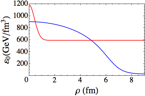
Figure 4.2: The initial energy density profiles at $\tau_{in}=0.12$ fm as a function of the distance to the origin. The blue curve models a central heavy-ion collision; the red curve models a fluctuation in such a collision.

Our model basically contains two scales: the initial energy density and the characteristic scale in the radial direction. We can, however, make use of the scale invariance of the field theory to rescale our coordinates such that at $\tau=0.6$ fm the energy density at the origin equals $\varepsilon_{0}=187\,\text{GeV/fm}^{3}$. We choose this combination to reproduce the final multiplicities of central heavy-ion collisions at LHC [122]. For the radial profile we then consider two types of initial conditions, specified at some small time $\tau_{in}\approx 0.12$ fm . The first is a model for a head-on collision, where the shape of the energy density is provided by the Glauber model, having an approximate radius of 6.5 fm. The second energy density profile models one fluctuation in the initial state of such a collision. We take a Gaussian of width 0.5 fm for this profile (see figure 4.2). For both initial conditions we assume that initially there is no radial momentum, such that $f_{4}(\tau_{in},\,\rho)=0$.

Importantly, we must also specify the metric functions $B(r,\,\tau_{in},\,\rho)$ and $C(r,\,\tau_{in},\,\rho)$ on a full time-slice of the bulk AdS geometry. These two functions, together with $a_{4}$, $f_{4}$ and the Einstein equations, specify the complete metric and its time derivative on a time-slice. In principle, these functions should follow from a model describing the very first less strongly coupled stage after the collision, such as the Glauber model or the Color Glass Condensate. However, these models themselves contain significant uncertainties and, more importantly, it is not clear how to map them to this gravitational setting. Refining our initial conditions in the next section, we will restrict ourselves here with a simple choice, where $B$ and $C$ are the same functions as in vacuum AdS, but with modified $b_{4}$ and $c_{4}$, such that the longitudinal pressure $p_{y}$ vanishes initially:

$$B(r,\,\tau_{in},\,\rho)=C(r,\,\tau_{in},\,\rho)=-\frac{2}{3}\log((\tau+1/r)\rho)-\frac{1}{8}a_{4}(\tau_{in},\,\rho)/r^{4}.$$ (4.1.6)

Having specified the initial and boundary conditions we can solve Einstein’s equations (see Appendix A) numerically , using essentially the same scheme as in chapter 3. One difference is the required boundary conditions in the $\rho$ direction, which in this case means smoothness at the origin and at infinity. Also the condition for the apparent horizon changes slightly, becoming

$$3S^{2}\dot{S}-\partial_{z}\left(S\,F\,e{}^{-B}\right)+\frac{3}{2}e^{-B}F^{2}S^{\prime}=0,$$ (4.1.7)

and lastly we used a grid in the $\rho$ direction parametrised by $\rho=L\frac{x}{(1-x^{2})^{1/\#}}$, where $x$ ranges from 0 to 1, and $\#$ is 20 and 4 for the nucleus and fluctuation model respectively. Typically around 35 grid points in both directions are used, and we choose $L=18$ or $L=2$ for the nucleus and fluctuation models respectively. Complicating the implementation somewhat, all quantities were again modified to be finite and non-trivial at the boundary, where in this case also $\rho=0$ is included as a boundary.

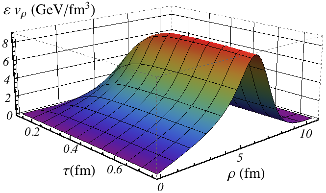
Figure 4.3: The radial velocity times the energy density as a function of proper time $\tau$ and distance to the origin $\rho$ for our model of a nucleus. Note that at late times the increasing velocity is almost exactly compensated by the decreasing energy density (which is due to the longitudinal expansion). The slope at the origin at the end of our simulation equals 0.66 GeV/$\text{fm}^{4}$.

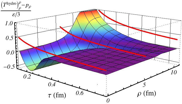
Figure 4.4: The difference between the full non-equilibrium $p_{\rho}$ and the pressure given by first order hydrodynamics. Although hydrodynamics applies very quickly, the viscous contribution is still large (shown by a red lines). The relatively high values for $\rho>7$ fm are a consequence of the very small energy density. For the model of a fluctuation the graph is similar, with equally quick thermalisation.

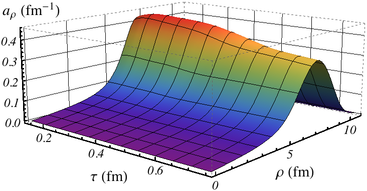
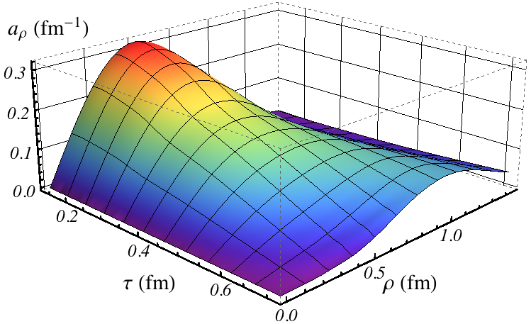
(a)	(b)

Figure 4.5: (a) The radial acceleration of our nucleus model. The acceleration decreases after some time, which is mainly a consequence of the decrease in radial pressure, due to the isotropisation. Thereafter the acceleration is quite steady and mainly localised near the boundary of the nucleus. (b) The radial acceleration of our fluctuation model. Since the bump of energy is much smaller one can clearly see the spreading out and the decrease in acceleration. As will also be clear from figure 4.6, this model reaches a lower radial speed than the model for the nucleus.

After determining the stress tensor one can extract the radial velocity, defined again by the boost after which there is no momentum flow. Figure 4.3 shows this velocity times the energy density, which gives a good measure of the momentum flow. The radial velocity, together with the stress tensor in the local rest frame, can be used to compute the stress tensor according to hydrodynamics. Although initially there will not be local equilibrium, at late times a hydrodynamic expansion is expected to be valid. It is therefore interesting to compare the actual pressures with the pressures which follow from a hydrodynamic expansion [18, 71], analogously to subsection 3.1.4.

In figure 4.4 we plot the difference of $p_{\rho}$ and the corresponding first order hydrodynamic prediction of our model of a nucleus. The stress tensor is excellently described by hydrodynamics as soon as $\tau=0.35$ fm. At the border of our nucleus this is slightly subtler, since the stress tensor is rather small there, and it becomes comparable to our regulator energy density. We therefore cannot say too much about this, but the agreement with hydrodynamics is also there encouraging. We note that in previous studies [40, 57] somewhat larger thermalisation times (with respect to the local temperature) were found, so we expect more exotic initial conditions in our bulk AdS to give somewhat later thermalisation.

In figure 4.5b we plot the radial acceleration of our model of a fluctuation. We notice the acceleration already decreases considerably during our simulation, in contrast with the model for the nucleus (figure 4.5a). Also, the acceleration increases rapidly near the origin, whereas for the nucleus it is rather narrowly peaked near the boundary of the nucleus. This means that fluctuations are expected to spread out rather quickly. Perhaps surprisingly, also the stress tensor for the fluctuation is governed by hydrodynamics within 0.35 fm.

The main motivation for the two examples above is to provide a description of the far-from-equilibrium stage of heavy-ion collisions, including non-trivial dynamics in the transverse plane. While we kept rotational symmetry in the transverse plane, we believe our study can be used more generally. One reason for this is an old result in asymptotically flat space [63], recently studied in asymptotically AdS ([57] and section 2.2), that during black hole formation gravity can be well approximated by linearising around the final state. We therefore believe that an initial energy profile with many fluctuations could be well approximated by superposing the result of our fluctuation presented above.

Also, it should be possible to use our results for non-central collisions. This can be seen by comparing with a formula for universal initial flow [123]. There, they assume that the anisotropy is independent of $\rho$, the transverse pressures are equal and that the velocity is approximately linear in time. Without using any hydrodynamics, they used the conservation of the stress tensor to arrive at the following local formula for the transverse momentum of the stress tensor:

$$\vec{s}/\varepsilon\approx-\frac{\vec{\nabla}_{\perp}\varepsilon_{0}}{2\varepsilon_{0}}(\tau-\tau_{in}),$$ (4.1.8)

where $\varepsilon_{0}$ is the initial energy density. This formula (see fig. 4.6) works remarkably well at early times and also later on for the nucleus model. At later times the transverse velocities of fluctuations are smaller, which is due to the decreasing acceleration (displayed in figure 4.5b). This result therefore increases confidence in the result of [123], which can be used in less symmetric situations. When including fluctuations, however, one should hydrodynamics as soon as $\tau=0.4$ fm to get more accurate results.

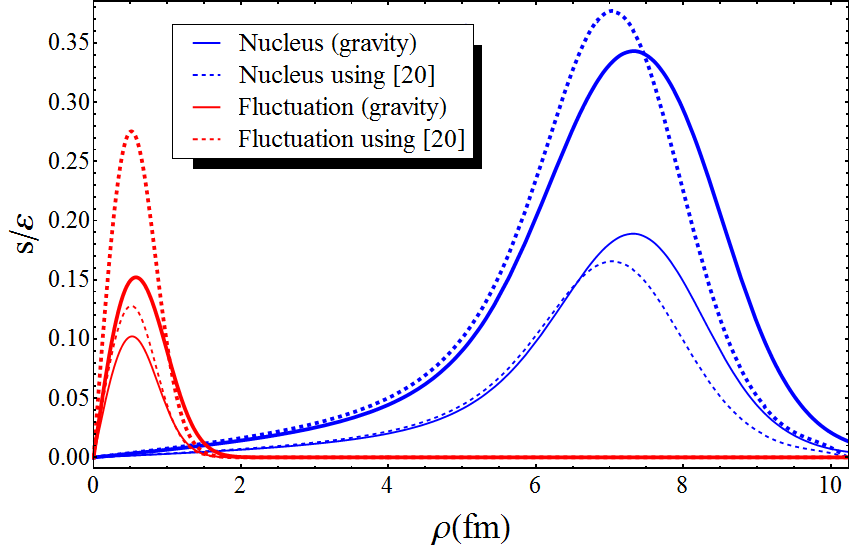
Figure 4.6: Here we plot the momentum flow $s$ divided by the energy density, at time $\tau=0.75$ fm (thick lines) and $\tau=0.4$ fm (thin lines), as a function of $\rho$. The plots compare our gravitational results with formula 4.1.8, which was found in [123]. The two results are remarkably similar, especially at earlier times, and considering the dynamics takes place at very different scales. We suggest formula 4.1.8 as an initial condition for non-symmetric hydrodynamic simulations, where a simulation should start at about $\tau=0.4$ fm if fluctuations are present.

4.2 A fully dynamical simulation of central nuclear collisions

In this section we attempt to obtain initial conditions by including the far-from-equilibrium stage obtained from colliding shock waves in AdS. After the matter has equilibrated, we match the AdS/CFT results onto a standard viscous hydrodynamics code which, once the matter has cooled below the QCD phase transition temperature $T_{c}$, is itself matched onto a standard hadronic cascade code, thereby achieving a fully dynamical simulation of a boost-invariant heavy-ion collision.

As in eqn. 3.2.2 and section 4.1, the main physical input for our simulation will be the energy density of a highly boosted and Lorentz contracted nucleus, $T_{tt}=\delta(t+z)T_{A}(\rho)$, with the “thickness function”

$$T_{A}(\rho)=\epsilon_{0}\int_{-\infty}^{\infty}dz\left[1+e^{(\sqrt{\rho^{2}+z^{2}}-R)/a}\right]^{-1}\,,$$ (4.2.1)

where $R=6.62$ fm, $a=0.546$ fm for a ${}^{208}{\rm Pb}$ nucleus[76]. The normalization $\epsilon_{0}$ is a measure of the energy of the nucleus, and given the simplicity of our model, we will use this constant to match the experimentally observed number of particles (“multiplicity”, $dN/dY$). It is noteworthy that analogously to subsection 3.2.1 we could match $\epsilon_{0}$ to energies used at LHC. This, however, would lead to $\epsilon_{0}$ being more than a hundred times bigger than what we will find, which is perhaps unsurprising in our simple model with boost-invariance.

Here we again describe a relativistic nucleus as a gravitational shockwave in AdS, whereby the stress-energy tensor of a nucleus can be exactly matched to the thickness function. For a head-on (central) collision this shockwave collision has been written down and solved near the boundary of AdS in Ref. [119], resulting in the stress-energy tensor at early times to leading order in $t$ that reads

$$e=2T_{A}^{2}(\rho)\tau^{2}\,,\ u^{\rho}=-\frac{T_{A}^{\prime}(\rho)}{3T_{A}(\rho)}\tau\,,\ \frac{P_{L}}{P_{T}}=-\frac{3}{2},\quad$$ (4.2.2)

where in the local rest frame $T_{\nu}^{\mu}={\rm diag}(-e,\,P_{T},\,P_{T},\,P_{L})$ and $u^{\mu}$ is defined as in 1.3.1. The velocity dependence and pressure anisotropy are consistent with our numerical computations (figure 3.5) and the universal flow formula 4.1.8. The early time result (4.2.2) fixes the first few near-boundary series coefficients of $B$ and $C$, but does not fix the metric functions deep in the bulk, leading to an unstable time evolution. In order to have a stable time evolution, we introduce a function with one bulk parameter $\sigma$ to extend the metric functions to arbitrary $r$, specifically choosing

$$B(r,\tau,\rho)\rightarrow B_{0}(r,\tau,\rho)+\sum_{i=0}^{6}\frac{b_{i}(\tau,\rho)r^{-i}}{1+\sigma^{7}r^{-7}}\,,$$ (4.2.3)

and analogously for $C$. Here $B_{0}(r,\,\tau,\,\rho)=-\frac{2}{3}\log((\tau+1/r)\rho)$ would give vacuum AdS, and the $b_{i}(\tau,\rho)$ are choosen such that the stress tensor 4.1.4 equals eqn. 4.2.2. Having $B$, $C$, $a_{4}$ and $f_{4}$ at a time $\tau_{{\rm init}}$ and choosing a value for $\sigma$, the future metric is completely determined by the same method as in section 4.1.

From the metric we again extract the full $T^{\mu\nu}$ (eqn. 4.1.4) and in particular observe the transition from early-time, far-from equilibrium dynamics to a fluid described by viscous hydrodynamics. At some value of proper time $\tau_{{\rm hydro}}$, we stop the evolution using Einstein equations and extract $e,\,u^{\mu},\,\pi^{\mu\nu}$ from eqn. 1.3.1. These functions provide the initial conditions for the well-tested relativistic viscous hydrodynamic code vh2 (version 1.0) [120], which uses an equation of state (EoS) inspired by lattice QCD and has, for simplicity, $\eta/s=\frac{1}{4\pi}$. Since this EoS differs from the conformal EoS of our AdS model there will be a discontinuity in the pressure. At high temperatures, however, QCD is approximately conformal and in our simulations the discontinuity at the center was never more than 15%.

The hydrodynamic code simulates the evolution from $\tau=\tau_{{\rm hydro}}$ until the last fluid cell has cooled down below $T_{{\rm sw}}=0.17$ GeV. The hydrodynamic variables along the hypersurface defined by $T=T_{{\rm sw}}$ are stored and converted into particle spectra using the technique from Ref. [121]. The subsequent particle scattering is treated using a hadron cascade [124] for resonances with masses up to $2.2$ GeV by simulating $500$ Monte-Carlo generated events. Once the particles have stopped interacting, and particles unstable under the strong force have decayed, light particle transverse momentum spectra are analyzed and can be compared to data.

From the hydrodynamic evolution onward our model uses techniques and parameters which are fairly standard. The initial conditions for hydrodynamics, however, are now determined using a far-from-equilibrium evolution. We modeled this phase as a strongly coupled CFT, described by gravity in AdS. This introduces new parameters and functions, namely the initialization time $\tau_{{\rm init}}$, the normalization $\epsilon_{0}$, the bulk function with parameter $\sigma$ and the AdS/hydro switching time $\tau_{{\rm hydro}}$. We will explore the effects of changing these parameters below.

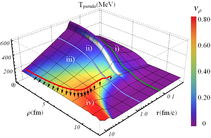
Figure 4.7: Assuming (1.3.1) applied, a “pseudo” temperature (defined by using Eq. (1.3.1) with $e=e(T_{{\rm pseudo}})$) and radial velocity $v_{\rho}=u_{\rho}/u_{\tau}$ are extracted for a representative simulation. The plot illustrates four physical tools used: i) early time expansion, ii) numerical AdS evolution, iii) viscous hydrodynamics until $T=0.17\,\text{GeV}$, iv) kinetic theory after conversion into particles (indicated by arrows). The (white) region close to $\tau\sim 0.2$ fm/c, $\rho\sim 5$ fm/c indicates a far-from-equilibrium domain where a local rest frame cannot be found.

4.2.1 Resulting particle spectra

Matching our numerical relativity, viscous hydrodynamics and hadron cascade simulations onto one another we obtain the time-evolution of the energy density for $Pb-Pb$ collisions at $\sqrt{s}=2.76$ TeV (see Fig. 4.7). The results depend on our choices of $\epsilon_{0},\tau_{{\rm init}}$ and $\sigma$, which are all parameters that in principle could be fixed by a more complete calculation. Requiring that for constant $\tau_{{\rm init}}$ and $\sigma$ our $dN/dY$ matches the experimental value fixes $\epsilon_{0}$. Different combinations of $\tau_{{\rm init}}$ and $\sigma$ will have similar late-time energy densities (cf. Fig. 4.8), but originate from different early-time histories and the pre-equilibrium evolution reported in Figs. 4.8,4.10 should be considered uncertain. However, we find that for fixed $dN/dY$ also the late time radial flow velocity and final light hadron spectra are essentially unaffected by our choice of $\tau_{{\rm init}}$ or $\sigma$ (see Figs. 4.8–4.12).

This is evident when comparing the resulting hydrodynamic radial velocity at $\tau=1$ fm/c shown in Fig. 4.9. Different values for $\tau_{{\rm init}},\,\tau_{{\rm hydro}}$ and $\sigma$ collapse onto an approximately universal velocity profile. Because the subsequent evolution follows hydrodynamics, this is also true for the velocity profile for all later times. We therefore expect our late time results to be robust.

One is not completely free in specifying $\tau_{{\rm init}}$ or $\sigma$. The coordinate singularity at $\tau=0$ prevents going to very early times, while one naturally has to start the AdS/CFT code long before the time hydrodynamics is expected to be applicable. In practice we found $0.07\leq\tau_{{\rm init}}({\rm fm)\leq 0.17}$ to be a good range. For $\sigma$ one has to make sure the AdS spacetime is sufficiently regular to allow for a stable evolution. In practice, we found $7.5\leq\sigma({\rm fm}^{-1})\leq 14$ to work well.

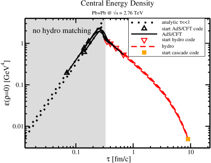
Figure 4.8: Time evolution of the energy density at the center of the fireball for different values of the regulator $\sigma$, different AdS/CFT starting times $\tau_{{\rm init}}$ and different AdS/hydro switching times $\tau_{{\rm hydro}}$. Shown are the analytic early time result (dotted), the numerical AdS/CFT evolution (full lines), the numerical hydro evolution (dashed lines) and the conversion point to the hadron cascade. For $\tau\lesssim 0.35$ fm/c, no sensible matching from AdS/CFT to a hydrodynamic evolution is possible (“no hydro matching”), cf. Fig. 4.10.

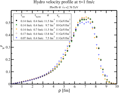
Figure 4.9: Radial velocity profile at $\tau=1$ fm/c for different AdS/CFT starting times $\tau_{{\rm init}}$, different AdS/hydro switching times $\tau_{{\rm hydro}}>0.35$ and different values for the regulator $\sigma$ (in a.u.). One observes that when normalized to the same final multiplicity, all these choices lead to similar velocity profiles.

The time evolution of the pressure anisotropy shown in Fig. 4.10 indicates a strongly varying, and occasionally negative, longitudinal pressure prohibiting any hydrodynamic description for $\tau<0.35$ fm/c. Besides the strongly varying anisotropy, we also typically encounter a closed region in space-time where the system is so far from equilibrium that a local rest frame does not seem to exist, which we plan to report on in future work. In principle, one could choose any value of $\tau_{{\rm hydro}}>0.35$ fm/c; however, switching at very late times $\tau_{{\rm hydro}}\gg 1$ fm/c is not recommended because of the prohibitive computational cost of the numerical relativity code and the fact that at later times the system has cooled down to temperatures where the QCD EoS is no longer close to the conformal EoS in the AdS/CFT code. For $\tau>0.35$ fm/c we can attempt to match the pre-equilibrium phase onto viscous hydrodynamics at $\tau=\tau_{{\rm hydro}}$, which surprisingly seems to lead to roughly similar final results even when $P_{L}\simeq 0$ (cf. Fig. 4.10). A more refined result can be gained by considering the dependence of the final light hadron spectra on the choice $\tau_{{\rm hydro}}$ discussed below.

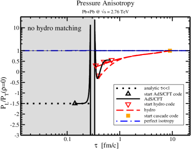
Figure 4.10: Time evolution of the pressure anisotropy $P_{L}/P_{T}$ at the center of the fireball for single values of $\sigma,\tau_{{\rm init}}$ but multiple AdS/hydro switching times $\tau_{{\rm hydro}}$. For $\tau\lesssim 0.35$ fm/c, the pressure anisotropy is wildly varying, prohibiting a sensible matching to hydrodynamics. At later times, matching to hydrodynamics can be performed (indicated by triangles down) and leads to approximately universal late-time evolution until freeze-out to the hadron cascade (indicated by square).

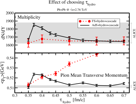
Figure 4.11: Final $dN/dY$ and pion $\langle p_{T}\rangle$ as a function of the hydro switching time $\tau_{{\rm hydro}}$ for a single value of $\sigma,\tau_{{\rm init}}$ (AdS+hydro+cascade) compared to experimental data (ALICE [125]). AdS results seem to be independent of $\tau_{{\rm hydro}}$ provided that $\tau_{{\rm hydro}}>0.5$ fm/c. By contrast, results for FS models with $\tau_{{\rm init}}=0.05$ fm/c exhibit strong $\tau_{{\rm hydro}}$ dependence. Error bars correspond to accumulated numerical error.

In order to compare our thermalising strongly coupled model we have considered two other (extreme) possibilities for the initial stage before $\tau_{hydro}$. The first has $P_{L}=0$, which gives zero coupling boost-invariant free streaming (FS), whereas the second has $P_{T}=0$, which hence has zero pre-equilibrium radial flow (ZF). These models never lead to thermalisation, but operationally one can switch to hydrodynamics at some time $\tau_{{\rm hydro}}$.

Fig. 4.11 shows the dependence of the final multiplicity and pion mean transverse momentum on the hydro switching time $\tau_{{\rm hydro}}$ for the AdS and FS models. For the final stage hadron cascade only hydro information for $\tau>1$ fm/c is used. Fig. 4.11 indicates that final $dN/dY,\langle p_{T}\rangle$ in our AdS model are constant, provided one switches to hydrodynamics after the far-from-equilibrium regime has ended (at about $\tau\approx 0.5$ fm/c). This suggests that our model reaches hydrodynamics dynamically and hence is insensitive to the choice of $\tau_{{\rm hydro}}$.

In contrast, for the FS and ZF models $\langle p_{T}\rangle$ depends on $\tau_{hydro}$, which hence only reproduces the data for a specific value, not following from a theoretical calculation. So while measured particle spectra do not rule out these models, the AdS model has the conceptual advantage of naturally leading to hydrodynamics, thereby making the model more constrained.

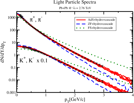
Figure 4.12: Pion and Kaon momentum spectra for 0-5% most central $Pb+Pb$ collisions at $\sqrt{s}=2.76$ TeV. Experimental measurements (ALICE [125]) are compared to our AdS+hydro+cascade model (lines correspond to different choices of $\epsilon_{0},\sigma$), the ZF model initialized from eqn. (4.2.1) at $\tau_{{\rm hydro}}=1$ fm/c, and the FS model with $\tau_{{\rm hydro}}=0.5$ fm/c.

In Fig. 4.12 we show the results for the final pion and kaon transverse momentum spectra in comparison to data for central $Pb+Pb$ collisions at $\sqrt{s}=2.76$ TeV from the ALICE experiment [125]. The integral over the momentum spectra corresponds to the total multiplicity which we fixed by hand. However, Fig. 4.12 shows that our AdS+hydro+cascade model matches the shape of the experimental data almost perfectly up to the highest transverse energies measured, independent of our choices for $\tau_{{\rm init}},\,\tau_{{\rm hydro}}$ and $\sigma$.

In this section we have presented a fully dynamical multi-physics simulation of central nuclear collision at LHC energies. This simulation includes a simulation of the equilibration of the bulk of the system using the AdS/CFT correspondence. When normalized to the same multiplicity, our framework is approximately insensitive to the AdS initialization time $\tau_{{\rm init}}$, the choice of bulk parameter $\sigma$ and the AdS/hydro switching time $\tau_{{\rm hydro}}$, provided the switching occurs later than $\sim 0.5$ fm/c. This is in constrast to non-thermalising models such as FS+hydro+cascade where results depend on choices for $\tau_{{\rm init}},\,\tau_{{\rm hydro}}$.

Because of the dynamical treatment of the pre-equilibrium stage and the insensitivity to our free parameters, our model is more constrained than a standard hydro+cascade model. In particular, we find that the transverse pressure is consistently higher than the longitudinal pressure, during most of the evolution (Fig. 4.10). Very encouragingly, the model turns out to have light particle spectra in excellent agreement with experimental data for $Pb+Pb$ collisions at $\sqrt{s_{NN}}=2.76$ TeV.

We regard this work as the first step towards a truly realistic simulation of high energy nuclear collisions. Many aspects of our work can and should be improved in future work. For instance, we plan to do away with the bulk parameter $\sigma$ by simulating the full shock-wave collision process (cf. chapter 3) and simulate event-by-event non-central collisions by employing a linearised scheme. The latter would allow comparison of both $\langle p_{T}\rangle$ and angular correlations, thereby giving an even more meaningful comparison of our model with experimental nucleus-nucleus or proton-nucleus data [126, 93, 127, 128].

Chapter 5 Conclusion and discussion

In the preceding chapters three main lessons were learnt

1. A homogeneous strongly coupled conformal plasma starting in general far-from-equilibrium states will thermalise very quickly, meaning that hydrodynamics is applicable within a time $\sim 1/T$, with $T$ the local temperature. Furthermore, linearising the initial state around the final state can provide a much simpler and relatively accurate description.

2. The longitudinal dynamics in a collision of gravitational shock waves provides rich physics; if the shocks are wide relative to the energy content, they will thermalise during the collision, come to a stop, and explode hydrodynamically. If they are thin, however, they do not have time to thermalise, but they pass right through each other, leaving behind a plasma later on with a characteristic rapidity profile (section 3.4). In the latter case this profile is insensitive to the microstructure of the shock wave: the shock waves act coherently. In particular, this implies a universal shape of the rapidity profile at high energies, which has experimental implications outlined in this thesis.

3. Assuming boost-invariance in the longitudinal direction, it was possible to realistically model a central heavy-ion collision in AdS/CFT. It was shown explicitly that AdS/CFT continuously links far-from-equilibrium dynamics with hydrodynamics, which is generally hard in other approaches. The resulting particle spectra match LHC data well, perhaps unreasonably well.

Alongside these lessons special attention was paid to clarify the set-up used for these problems in numerical relativity. They turn out to be much simpler than typical problems in numerical relativity, such as the merger of black hole. After the relatively straightforward addition of electromagnetic and scalar fields this method is expected to be useful in far more general settings within AdS/CFT, such as in the context of holographic superconductors or other holographic condensed matter studies [129, 130, 131].

5.1 A comparison with experiments?

In this thesis we have made an effort to compare our results with experimental data, in particular high-lighting a major difference in the rapidity distribution of proton-nucleus collisions computed using perturbative QCD or our strongly coupled method (subsection 3.3.1). Nevertheless it is clear that all computations have been done in an oversimplified setting. We tried to approximate real-world asymptotically free QCD with a conformal theory, $\mathcal{N}=4$ SYM, notably at infinitely strong coupling and with an infinite number of colours. Only gravity was considered, whereas other forces may be relevant when modelling heavy-ion collisions. Note, however, that gravity is the only force which gets stronger with increasing energy classically. It is therefore expected that at high energy heavy-ion collisions gravity is the dominant force. Furthermore, lattice QCD computations have shown that QCD behaves very similarly when increasing the number of colours, thereby validating the assumption of a large number of colours [132].

There is one other good argument to believe a relatively simple model could capture many features of real collisions, which is the fortunate separation of three scales: $1/T\ll r_{nucleon}\ll r_{nucleus}$, with $T\sim 1/(0.1\text{fm})$ the local temperature at thermalisation, $r_{nucleon}\approx 0.9$ fm the radius of a nucleon and $r_{nucleus}\approx 6.7$ fm the radius of a nucleus. This separation can be very helpful in a realistic dual of QCD; there one may imagine to model each nucleon as a source at a AdS radial position of about $1$ fm, where we used the scale/radius duality. Alternatively we could place the sources at about $1/T_{QCD}\approx 1.2$ fm, with $T_{QCD}$ the QCD deconfinement temperature. After some nucleons collide a horizon would form at a depth of about $1/T\sim 0.1$ fm, thereby completely hiding the original sources behind the horizon, making their details of little importance. On the other hand, the nucleus itself is much bigger (14 fm) than the depth of the sources. This allows the horizon to fall off outside the collision region sufficiently fast such that nucleons not directly involved in the collision (spectators) can move on almost unperturbed. Furthermore, the relatively big size of the nucleus makes it likely that transverse dynamics can be treated independently of longitudinal dynamics during the initial stage.

The above discussion does not say much about the difference between an infinite coupling constant and the real-world QCD coupling constant, which goes to zero at asymptotically high energies. At energies at RHIC and LHC the QCD coupling is presumably not yet very weak, as otherwise the success of hydrodynamic modelling of heavy ion and more recently proton-lead collisions would be hard to explain. Nevertheless, there is little reason to expect an infinite coupling approximation to be valid. In fact, we believe that especially the total multiplicities found in subsection 3.4.2 suggest that at infinite coupling there is more stopping than what is found in LHC measurements. It is only natural that finite coupling corrections would reduce the stopping, thereby getting closer to experimental data. Presumably, this will reveal itself as a widening of the rapidity profile (section 3.4), which we found to be universal at high energy and infinite coupling.

5.2 Future directions

Properly taking into account finite coupling effects within AdS/CFT would most likely be the most promising avenue to make a more precise link with experiments. Some efforts have been made by modifying the UV geometry or including finite coupling effects in simple models of thermalisation [110, 112, 133, 134]. It may also be necessary to critically compare the field content of theories in AdS with QCD. It is generally believed that gluons dominate most of the dynamics in both theories, but other fields definitely play a role. In particular, it may be that quarks in QCD require a different description than the one presented in this thesis.

On the other hand one may take a more phenomenological approach, which has been the main motivation for chapter 4. There, we fitted the normalisation of the initial energy density in order to match the total multiplicity. This fitting parameter indeed turned out to be significantly different from the energy density we would have found using a more complete calculation such as for instance the colliding shock waves of chapter 3. Optimistically one could therefore say that fitting the normalisation of the energy density takes into account weak-coupling effects, and in this specific case also violations of boost-invariance. We found that this approach has appealing features, being most importantly the dynamical transition to hydrodynamics and the almost perfect fit of LHC measurements.

So in future we will most likely combine several of these ideas. It would be good to try and do a full first principle finite coupling calculation, but at the same time a lot can be achieved by using more phenomenological inspired techniques. In particular, it would be interesting to relax the rotational and boost symmetry imposed in chapter 4, perhaps using a linearised approximation. It will also be worthwhile to combine this study of thermalisation with other observables, most notably the quenching of jets, or the production of photons.

Lastly, we would like to reiterate our introductory statement that experimental heavy-ion data are highly constraining, and in future this will lead to a much more complete understanding of the quark-gluon plasma and QCD in general. We hope that our strongly coupled AdS/CFT approach will be part of that understanding.

Appendix

Here we write out the explicit form of the geodesic equations used in subsection 3.1.1

$$\begin{array}[]{c}\frac{\left(a^{\prime}(\lambda)+1\right)^{2}+b^{\prime}(\lambda)c^{\prime}(\lambda)}{a(\lambda)+\lambda}=\frac{\lambda a^{\prime\prime}(\lambda)+2a^{\prime}(\lambda)-h\lambda(a(\lambda)+\lambda)^{3}b^{\prime}(\lambda)^{2}+2}{\lambda}\\ \frac{2\left(a(\lambda)-\lambda a^{\prime}(\lambda)\right)b^{\prime}(\lambda)}{\lambda(a(\lambda)+\lambda)}+b^{\prime\prime}(\lambda)=0\\ 8h(a(\lambda)+\lambda)^{3}\left(a^{\prime}(\lambda)+1\right)b^{\prime}(\lambda)+\frac{2\left(\lambda a^{\prime}(\lambda)-a(\lambda)\right)c^{\prime}(\lambda)}{\lambda(a(\lambda)+\lambda)}+(a(\lambda)+\lambda)^{4}b^{\prime}(\lambda)^{2}h^{\prime}=c^{\prime\prime}(\lambda),\end{array}$$ (5.2.1)

where $h\equiv h[t+z+b(\lambda,\,t)]$ and we suppressed the time dependence of $a$, $b$ and $c$, present through their boundary conditions.

The Einstein equations for the shock wave collisions in chapter 3 can be reduced to [39]:

$$\begin{array}[]{ccc}S^{\prime\prime}&=&-\frac{1}{2}SB^{\prime 2}\\ S^{2}F^{\prime\prime}&=&S\left(6\tilde{S}B^{\prime}+4\tilde{S}^{\prime}+3F^{\prime}S^{\prime}\right)+S^{2}\left(3\tilde{B}B^{\prime}+2\tilde{B}^{\prime}\right)-4\tilde{S}S^{\prime}\\ 12S^{2}\dot{S}^{\prime}&=&e^{2B}\left(S\left(4\tilde{B}F^{\prime}-7\tilde{B}^{2}-4\tilde{\tilde{B}}+2\tilde{F}^{\prime}+F^{\prime 2}\right)+2\tilde{S}\left(F^{\prime}-8\tilde{B}\right)-8\tilde{\tilde{S}}+8\tilde{S}^{2}\right)+24S\left(S^{2}-\dot{S}S^{\prime}\right)\\ 6S^{3}\dot{B}^{\prime}&=&e^{2B}\left(S\left(-\tilde{B}F^{\prime}+\tilde{B}^{2}+\tilde{\tilde{B}}-2\tilde{F}^{\prime}-F^{\prime 2}\right)+\tilde{S}\left(\tilde{B}+4F^{\prime}\right)+2\tilde{\tilde{S}}-4\tilde{S}^{2}\right)-9S^{2}\left(\dot{S}B^{\prime}+\dot{B}S^{\prime}\right)\\ 2S^{3}A^{\prime\prime}&=&e^{2B}\left(S\left(7\tilde{B}^{2}+4\tilde{\tilde{B}}-F^{\prime 2}\right)+16\tilde{B}\tilde{S}+8\tilde{\tilde{S}}-32\tilde{S}^{2}\right)-2S^{3}\left(3\dot{B}B^{\prime}+4\right)+24\dot{S}SS^{\prime}\\ 6S^{2}\dot{F}^{\prime}&=&3\left(8\dot{S}\tilde{S}+2S\left(S^{\prime}\left(\tilde{A}+2\dot{F}\right)-6\dot{B}\tilde{S}-4\tilde{\dot{S}}-3\dot{S}F^{\prime}\right)-S^{2}\left(2B^{\prime}\left(\tilde{A}+2\dot{F}\right)+2\tilde{A}^{\prime}+6\dot{B}\tilde{B}+4\tilde{\dot{B}}+A^{\prime}F^{\prime}\right)\right)\\ 6S^{2}\ddot{S}&=&e^{2B}\left(S\left(2\tilde{B}\left(\tilde{A}+2\dot{F}\right)+\tilde{\tilde{A}}+2\tilde{\dot{F}}\right)+\tilde{S}\left(\tilde{A}+2\dot{F}\right)\right)+3S^{2}\left(\dot{S}A^{\prime}-\dot{B}^{2}S\right),\end{array}$$ (5.2.2)

where $h^{\prime}=\partial_{r}h$, $\dot{h}=\partial_{t}h+\frac{1}{2}Ah^{\prime}$ and $\tilde{h}=\partial_{y}h-Fh^{\prime}$. Note that these operators do not commute and so that one has to be careful that $\tilde{h}^{\prime}=(\tilde{h})^{\prime}$.

The Einstein equations for the radial expanding plasma in chapter 4 can be reduced to:

$$\begin{array}[]{ccc}3S^{\prime\prime}&=&-\frac{1}{6}S\left(B^{\prime}C^{\prime}+\left(B^{\prime}\right)^{2}+\left(C^{\prime}\right)^{2}\right)\\ 2S^{2}F^{\prime\prime}&=&S^{2}\left(\tilde{B}\left(2B^{\prime}+C^{\prime}\right)+\tilde{C}\left(B^{\prime}+2C^{\prime}\right)-2\tilde{B}^{\prime}\right)+S\left(-6\tilde{S}B^{\prime}+8\tilde{S}^{\prime}+6F^{\prime}S^{\prime}\right)-8\tilde{S}S^{\prime}\\ 12S^{3}\dot{S}^{\prime}&=&e^{-B}\left(-S^{2}\left(\tilde{B}\left(\tilde{C}+2F^{\prime}\right)-2\left(\tilde{\tilde{B}}+\tilde{F}^{\prime}-12e^{B}\dot{S}S^{\prime}\right)+2\tilde{B}^{2}+\tilde{C}^{2}-\left(F^{\prime}\right)^{2}\right)+2S\left(\tilde{S}\left(4\tilde{B}+F^{\prime}\right)-4\tilde{\tilde{S}}\right)+4\tilde{S}^{2}+24e^{B}S^{4}\right)\\ 6S^{3}\dot{C}^{\prime}&=&e^{-B}\left(S\left(2\tilde{B}\left(2\tilde{C}+F^{\prime}\right)+2\tilde{B}^{2}-2\tilde{\tilde{B}}+3\tilde{C}F^{\prime}+\tilde{C}^{2}-3\tilde{\tilde{C}}-2\tilde{F}^{\prime}-F^{\prime 2}\right)+\tilde{S}\left(4F^{\prime}-2\tilde{B}-3\tilde{C}\right)+2\tilde{\tilde{S}}-4\tilde{S}^{2}\right)-9S^{2}\left(\dot{S}C^{\prime}+\dot{C}S^{\prime}\right)\\ 6S^{4}\dot{B}^{\prime}&=&e^{-B}\left(-S^{2}\left(\tilde{B}\left(2\tilde{C}+F^{\prime}\right)+\tilde{B}^{2}-\tilde{\tilde{B}}+2\tilde{C}^{2}-4\tilde{F}^{\prime}-2F^{\prime 2}\right)+S\left(\tilde{S}\left(\tilde{B}-8F^{\prime}\right)-4\tilde{\tilde{S}}\right)+8\tilde{S}^{2}-9e^{B}S^{3}\left(\dot{S}B^{\prime}+\dot{B}S^{\prime}\right)\right)\\ 2S^{4}A^{\prime\prime}&=&e^{-B}\left(S^{2}\left(\tilde{B}\tilde{C}+2\tilde{B}^{2}-2\tilde{\tilde{B}}+\tilde{C}^{2}+24e^{B}\dot{S}S^{\prime}-\left(F^{\prime}\right)^{2}\right)+8S\left(\tilde{\tilde{S}}-\tilde{B}\tilde{S}\right)-4\tilde{S}^{2}-e^{B}S^{4}\left(\dot{B}+\dot{C}\left(B^{\prime}+2C^{\prime}\right)+8\right)\right)\\ 2S^{2}\dot{F}^{\prime}&=&8\dot{S}\tilde{S}-S^{2}\left(2\tilde{A}^{\prime}-B^{\prime}\left(\tilde{A}+2\dot{F}\right)+\tilde{B}\left(2\dot{B}+\dot{C}\right)+\tilde{C}\left(\dot{B}+2\dot{C}\right)-2\tilde{\dot{B}}+A^{\prime}F^{\prime}\right)+2S\left(S^{\prime}\left(\tilde{A}+2\dot{F}\right)+3\dot{B}\tilde{S}-4\tilde{\dot{S}}-3\dot{S}F^{\prime}\right)\\ 6S^{2}\ddot{S}&=&e^{-B}\left(S\left(\tilde{B}\left(-\left(\tilde{A}+2\dot{F}\right)\right)+\tilde{\tilde{A}}+2\tilde{\dot{F}}\right)+\tilde{S}\left(\tilde{A}+2\dot{F}\right)+3e^{B}\dot{S}S^{2}A^{\prime}-e^{B}S^{3}\left(\dot{B}\dot{C}+\dot{B}^{2}+\dot{C}^{2}\right)\right),\end{array}$$ (5.2.3)

where now $\tilde{h}=\partial_{\rho}h-Fh^{\prime}$. Note that the tilded derivative $\tilde{h}$ does not actually simplify computations much as one still has to compute the tilded derivative explicitly. Here it just serves to present the equations more compactly. In the actual code all functions are regularised near the boundary, i.e. we redefine

$$A = r^{2}+\frac{Af}{r^{2}},$$

$$B = -\frac{2}{3}\log(\tau\rho)+\frac{3r\tau(1-2r\tau)-2}{9r^{3}\tau^{3}}+\frac{Bf}{r^{4}},$$

$$C = -\frac{2}{3}\log(\tau/\rho^{2})+\frac{3r\tau(1-2r\tau)-2}{9r^{3}\tau^{3}}+\frac{Cf}{r^{4}},$$

$$S = \rho^{1/3}\frac{3r\tau(9r\tau(3r\tau(3r\tau+1)-1)+5)-10}{243r^{3}\tau^{11/3}}+\frac{Sf}{r^{4}},$$

$$F = \frac{Ff}{r^{2}},$$ (5.2.4)

where all computations are then done with $Af$, $Bf$, $Cf$, $Sf$, $Ff$ and analogously $\dot{Bf}$ , $\dot{Cf}$ and $\dot{Sf}$, all depending on $r,\,\tau$ and $\rho$. The gauge freedom $\xi(\tau,\,\rho)$ is still suppressed, but can easily be reinstated by letting $r\rightarrow r+\xi(\tau,\,\rho)$ and redefining $A$ and $F$ appropriately. Although these redefinitions make the equations much longer, it has the advantage that one can easily and accurately extract the boundary stress tensor, without the need to compute derivatives.

Nederlandse samenvatting

De meeste mensen zullen denken dat de kleinste elementaire deeltjes weinig te maken hebben met de grootste en zwaarste objecten in ons heelal. Toch lijken ontdekkingen uit de snaartheorie hier wel op te wijzen. Niet letterlijk misschien, maar zwarte gaten kunnen een erg goed model vormen voor het gedrag van het quark-gluon plasma, zoals dat bij de LHC in Genï¿œve geproduceerd wordt.

Extremer kan het in de natuurkunde bijna niet worden; bij botsingen van loodkernen in de LHC onstaat voor ongeveer $10^{-23}$ seconde een plasma van quarks en gluonen met een temperatuur van $10^{12}$K en versnellingen van wel $10^{31}g$. Voeg hieraan toe dat dit proces misschien wel het best te beschrijven is met de vorming van een zwart gat in een 5 dimensionaal universum, waarbij het zwarte gat ongeveer de helft van dit universum inneemt, en het is duidelijk dat het hier om extreme natuurkunde gaat. In dit proefschrift wordt de relatie tussen loodkernen en zwarte gaten uitgelegd en wordt gekeken naar hoe we dit in praktijk kunnen gebruiken.

Holografie

Een oud idee uit 1974 van Gerard ’t Hooft [5] is dat quarks en gluonen, zoals beschreven door de Kwantumchromodynamica (QCD), equivalent kunnen zijn aan een theorie van snaren, waarbij de snaren tussen de quarks spannen. Toen al was duidelijk dat een dergelijke snaartheorie mogelijk kon worden versimpeld, maar de precieze uitwerking hiervan was erg ingewikkeld.

De doorbraak werd uiteindelijk in 1997 door Juan Maldacena gevonden [10], die een precieze snaartheorie vond die overeen kwam met een precieze kwantumtheorie. Deze kwantumtheorie heeft dan wel supersymmetrie, maar lijkt toch vrij veel op normale niet-supersymmetrische QCD. Achteraf gezien was er in 1974 allereerst veel meer kennis over snaartheorie nodig, maar een ander verrassend aspect was dat de snaartheorie ￜￜn extra ruimtelijke dimensie heeft: de snaartheorie is 4+1 dimensionaal, in tegenstelling tot de 3+1 dimensionale kwantumtheorie. Hierdoor heeft het de naam holografie gekregen.

Berekeningen in snaartheorie zijn ontzettend ingewikkeld, maar in de situatie dat de snaartjes heel klein zijn (puntdeeltjes) reduceert de snaartheorie tot normale , met zwaartekracht en de andere krachten. In deze limiet krijgen we een ‘normaal’ universum met onder andere zwarte gaten terug, maar dan wel met ￜￜn dimensie meer. In dit simpele geval is equivalente QCD juist (bijna) onmogelijk op te lossen, zodat een zwart gat echt een versimpeling voor het quark-gluon plasma is!

Botsingen van loodkernen

Eï¿œn maand per jaar botsen er in de Large Hadron Collider (LHC) loodkernen op elkaar. De rest van het jaar worden protonen gebotst die het meest bruikbaar zijn voor het vinden van het Higgsboson. Loodkernen zijn echter veel zwaarder dan protonen en aangezien de snelheid gelijk is, geeft deze botsing veel meer energie.

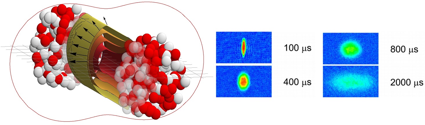
Figuur 5.1: Een botsing van twee loodkernen. In de regio waar de kernen overlappen onstaat een heet quark-gluon plasma, dat ongeveer ellipsvormig is. In de detector worden meer deeltjes gevonden in de richting van de korte as, wat geï¿œllustreerd wordt door de rode lijn. De expansie van het quark-gluon plasma zal nooit gefotografeerd worden, maar het lijkt veel op het rechter plaatje. Dit zijn moment opnames van bepaalde expanderende zeer koude atomen[135]. Het leuke hiervan is dat deze atomen net als het plasma door een moeilijke kwantumtheorie worden beschreven; het idee is dan ook dat ook hier zwarte gaten een model vormen voor deze vloeistof met zeer lage viscositeit. In zekere zin zijn de koudste en warmste vloeistoffen op aarde dus erg vergelijkbaar!

Met een paar honderd botsende energetische protonen en neutronen zou je kunnen verwachten dat alle deeltjes een paar keer botsen en in een betrekkelijk willekeurige richting in de detector belanden. Dit is echter niet wat in de LHC gevonden wordt; de deeltjes bewegen voornamelijk in de richting van de korte kant, zoals in figuur 5.1 geï¿œllusteerd. Deze zogenoemde ‘elliptic flow’ toont aan dat er veel interacties zijn, die de deeltjes in de x-as duwen.

Hoewel er nu veel experimentele data zijn, resteren nog veel open vragen over het quark-gluon plasma. Allereerst is het experimenteel een gigantische taak om naar het quark-gluon plasma te ‘kijken’. Het plasma zelf bestaat daar namelijk veel te kort voor en experimenteel zijn dus alleen de wegvliegende deeltjes lang na de botsing te detecteren. Hier zit echter een schat aan informatie in, zoals bijvoorbeeld de vorm van de distributie in figuur 5.1 afgebeeld. Maar ook het type deeltje, de snelheid, de verdeling in de z-richting en andere data kunnen allemaal nauwkeurig gemeten worden.

Een theoretische beschrijving

De uitdaging is uiteraard om al deze data theoretisch te voorspellen. Dit lukt heel aardig, maar er is een aantal cruciale aannames en waardes die moeilijk theoretisch te onderbouwen zijn. Het typische model is nu dat de individuele quarks en gluonen zich heel erg snel als een vloeistof gaan gedragen; daarna expandeert het plasma volgens relativistische hydrodynamica, met de kleinste viscositeit ooit gemeten (zie ook figuur 5.1). Het plasma wordt daarom ook wel de meest perfecte vloeistof genoemd. Op een gegeven moment is de energiedichtheid zo laag dat zo’n 30.000 deeltjes ontstaan, die dan nog weer veel later in de detector worden gemeten.

Het is met name erg moeilijk te beantwoorden waarom en hoe de deeltjes zo snel een vloeistof vormen. Ook de lage viscositeit is niet uit te rekenen binnen QCD. Holografie, echter, geeft op een heel natuurlijke wijze een lage viscositeit [30], aangezien in zekere zin ook de horizon van een zwart gat zich gedraagt als een perfecte vloeistof. Het hieronder gepresenteerde onderzoek probeert een (holografisch) beeld te vormen van de allereerste evolutie, nog voor de deeltjes een echte vloeistof vormen.

De formatie van zwarte gaten

Zoals eerder al geanticipeerd, is het erg moeilijk om met QCD precieze berekeningen te maken, in het bijzonder in de chaotische botsing van twee atoomkernen. Dit komt doordat QCD de sterke kracht beschrijft, die zo sterk is dat hij zich moeilijk laat benaderen.

Het mooie (en soms lastige) van holografie is dat als de kwantummechanische deeltjestheorie moeilijk is, de snaartheorie juist makkelijk is (en vice versa). In dit geval versimpelt snaartheorie naar klassieke zwaartekracht met eventueel andere krachten. Deze zwaartekracht, beschreven door Einsteins algemene relativiteitstheorie, zou dus goed een model kunnen vormen voor een moeilijke kwantumtheorie!

Het uitgangspunt in deze berekening is dat het quark-gluon plasma op een bepaalde manier goed beschreven kan worden door eigenschappen van de horizon van een zwart gat. De botsing zelf is dan equivalent aan de formatie van een zwart gat. Op een gegeven moment zal de horizon van dit zwarte gat goed worden beschreven door hydrodynamica en de grote vraag is hoe het plasma er op dat moment uitziet. Het gaat hierbij dan met name om wanneer hydrodynamica werkt en wat het snelheidsprofiel van de vloeistof op dat moment is.

Berekeningen in algemene relativiteitstheorie zijn een vakgebied op zichzelf, en het heeft daarom ook een tijd geduurd om de formatie van een zwart gat te beschrijven. In dit proefschrift is dit op een aantal manieren geprobeerd. Hoofdstuk 2 bestudeert het betrekkelijk triviale geval van een volledig homogeen zwart gat. Toch was dit al interessant, want hier kwam uit dat dit zwarte gat altijd erg snel door hydrodynamica beschreven wordt.

Hoofdstuk 3 beschrijft de botsing van schokgolven van zwaartekracht. In aanvulling op eerder werk [39] vonden we grote verschillen tussen schokgolven met veel en schokgolven met weinig energie. Met name dit eerste regime van hoge energie botsingen leidt tot interessante vergelijkingen met botsingen in LHC. Het belangrijkste resultaat is mogelijk een universeel snelheidsprofiel in de richting van de botsing (sectie 3.4), hetgeen fundamenteel anders is dan de twee bestaande profielen van Landau [95] en Bjorken [100].

Mogelijk het meest innovatief bestudeert hoofdstuk 4 een model dat dynamica en expansie in het vlak transversaal op de botsing heeft. Hoewel dit nog steeds rotatie-symmetrisch is, is het hiermee mogelijk met de uitkomsten in bestaande hydrodynamische modellen verder te rekenen. Dit leidde uiteindelijk tot meetbare deeltjesspectra, die verrassend goed overeenkomen met LHC meetresultaten (figuur 4.12).

Discussie

Hoewel veel technische details achterwege moesten blijven, is hopelijk toch duidelijk geworden waarom quarks en gluonen misschien wel het best door zwarte gaten beschreven kunnen worden. Eï¿œn van de leuke dingen hiervan is dat zwaartekracht in het algemeen ‘moeilijke’ kwantumtheorieï¿œn beschrijft, zoals het quark-gluon plasma, maar ook bijvoorbeeld bepaalde koude atomen (figuur 5.1). Doordat beide systemen door zwarte gaten beschreven kunnen worden, gedragen ze zich erg vergelijkbaar; iets wat erg onverwacht is voor de heetste en koudste vloeistoffen op aarde.

Holografie is essentieel gebleken om experimentele data van het quark-gluon plasma te verklaren. Een beschrijving in termen van zwarte gaten geeft hierbij een natuurlijke verklaring waarom het plasma zich zo snel als vloeistof gedraagt en waarom de viscositeit zo laag is. Met holografie is het nu ook mogelijk de allereerste momenten van de botsing te simuleren, als het plasma zich nog niet als een vloeistof gedraagt. Eï¿œn van de belangrijkste successen daarvan is een realistisch snelheidsprofiel, zowel in de richting van de botsing, als loodrecht daarop (hoofdstuk 3 en 4). Voor het loodrechte profiel blijkt dit goed overeen te komen met experimentele data, voor het longitudinale profiel is dit minder duidelijk (sectie 5.1).

Een heel ander recent succes is een model van zwarte gaten met supergeleiding [130]. In dit geval zijn het meer ingewikkelde zwarte gaten, met scalaire en elektrische velden. Deze extra’s leveren een ingewikkelder fasediagram op, waar ook een supergeleidende fase in blijkt te zitten. Hoewel het niet heel duidelijk is wat voor precieze kwantumtheorie zulke zwarte gaten zou moeten beschrijven, is er natuurlijk de hoop dat het iets te maken heeft met hoge temperatuur supergeleiders. Deze zijn nog erg slecht begrepen, ook weer omdat het een moeilijke kwantumtheorie betreft.

Het is ook leuk om op te merken dat holografie helemaal niet ontdekt is met oog op dit soort toepassingen vanuit de snaartheorie. Onderzoekers waren veelal geï¿œnteresseerd in het vinden van een ‘theorie van alles’. Hoewel holografie hier zeker aan bijdraagt, zal het misschien nog wel veel nuttiger blijken voor het begrijpen van ingewikkelde kwantumsystemen. En wie weet, begrijpen we uiteindelijk QCD, zwarte gaten of het mechanisme achter supergeleiding bij hoge temperatuur.

Curriculum Vitae

The author was born on February 3, 1987 in Wageningen, the Netherlands. He completed secondary school in 2004 at Het Streek in Ede, after which he moved on to study physics and mathematics at Utrecht University, obtaining bachelor’s degrees in both programmes in 2008 (cum laude). The next two years he continued there for a master’s degree (cum laude) in the programme Theoretical Physics, with a master thesis ‘Black holes as Information Scramblers’ supervised by prof. Gerard ’t Hooft.

From 2010 till 2014 the current PhD work was performed, under supervision of prof. Gleb Arutyunov, prof. Thomas Peitzmann and prof. Raimond Snellings, with the goal of bringing recent progress on heavy ion collisions using AdS/CFT closer to experiments. After obtaining his doctorate the author will continue his research at the Center of Theoretical Physics at the Massachusetts Institute of Technology in Cambridge, USA.

References

- [1] U. Heinz & R. Snellings, “Collective flow and viscosity in relativistic heavy-ion collisions”, Ann.Rev.Nucl.Part.Sci. 63, 123 (2013), arXiv:1301.2826.
- [2] STAR collaboration Collaboration, L. Adamczyk et al., “Inclusive charged hadron elliptic flow in Au + Au collisions at = 7.7 - 39 GeV”, Phys.Rev. C86, 054908 (2012), arXiv:1206.5528.
- [3] L. D. McLerran & R. Venugopalan, “Computing quark and gluon distribution functions for very large nuclei”, Phys.Rev. D49, 2233 (1994), hep-ph/9309289.
- [4] F. Gelis, “Color Glass Condensate and Glasma”, Int.J.Mod.Phys. A28, 1330001 (2013), arXiv:1211.3327.
- [5] G. ’t Hooft, “A Planar Diagram Theory for Strong Interactions”, Nucl.Phys. B72, 461 (1974).
- [6] J. D. Bekenstein, “Black holes and entropy”, Phys.Rev. D7, 2333 (1973).
- [7] G. Hooft, “Black Hole Quantization and a Connection to String Theory”, in “Physics, Geometry and Topology”, ed: H. Lee, Springer US (1990), p. 105-128.
- [8] G. ’t Hooft, “Dimensional reduction in quantum gravity”, gr-qc/9310026.
- [9] L. Susskind, “The World as a hologram”, J.Math.Phys. 36, 6377 (1995), hep-th/9409089.
- [10] J. M. Maldacena, “The Large N limit of superconformal field theories and supergravity”, AIP Conf.Proc. 484, 51 (1999).
- [11] E. Witten, “Anti-de Sitter space and holography”, Adv.Theor.Math.Phys. 2, 253 (1998), hep-th/9802150.
- [12] O. Aharony, S. S. Gubser, J. M. Maldacena, H. Ooguri & Y. Oz, “Large N field theories, string theory and gravity”, Phys.Rept. 323, 183 (2000), hep-th/9905111.
- [13] L. Susskind & E. Witten, “The Holographic bound in anti-de Sitter space”, hep-th/9805114.
- [14] E. Witten, “Anti-de Sitter space, thermal phase transition, and confinement in gauge theories”, Adv.Theor.Math.Phys. 2, 505 (1998), hep-th/9803131.
- [15] U. Gursoy & E. Kiritsis, “Exploring improved holographic theories for QCD: Part I”, JHEP 0802, 032 (2008), arXiv:0707.1324.
- [16] I. R. Klebanov & E. Witten, “AdS / CFT correspondence and symmetry breaking”, Nucl.Phys. B556, 89 (1999), hep-th/9905104.
- [17] A. Karch & E. Katz, “Adding flavor to AdS / CFT”, JHEP 0206, 043 (2002), hep-th/0205236.
- [18] R. Baier, P. Romatschke, D. T. Son, A. O. Starinets & M. A. Stephanov, “Relativistic viscous hydrodynamics, conformal invariance, and holography”, JHEP 0804, 100 (2008), arXiv:0712.2451.
- [19] W. A. Hiscock & L. Lindblom, “Generic instabilities in first-order dissipative relativistic fluid theories”, Phys.Rev. D31, 725 (1985).
- [20] R. Baier & P. Romatschke, “Causal viscous hydrodynamics for central heavy-ion collisions”, Eur.Phys.J. C51, 677 (2007), nucl-th/0610108.
- [21] M. P. Heller, R. A. Janik & P. Witaszczyk, “On the character of hydrodynamic gradient expansion in gauge theory plasma”, Phys.Rev.Lett. 110, 211602 (2013), arXiv:1302.0697.
- [22] K. S. Thorne, R. H. Price & D. A. MacDonald, “Black holes: the membrane paradigm”.
- [23] S. Bhattacharyya, V. E. Hubeny, S. Minwalla & M. Rangamani, “Nonlinear Fluid Dynamics from Gravity”, JHEP 0802, 045 (2008), arXiv:0712.2456.
- [24] V. E. Hubeny, S. Minwalla & M. Rangamani, “The fluid/gravity correspondence”, arXiv:1107.5780.
- [25] D. Mateos, “String Theory and Quantum Chromodynamics”, Class.Quant.Grav. 24, S713 (2007), arXiv:0709.1523.
- [26] S. S. Gubser & A. Karch, “From gauge-string duality to strong interactions: A Pedestrian’s Guide”, Ann.Rev.Nucl.Part.Sci. 59, 145 (2009), arXiv:0901.0935.
- [27] O. DeWolfe, S. S. Gubser, C. Rosen & D. Teaney, “Heavy ions and string theory”, Prog.Part.Nucl.Phys. 75, 86 (2014), arXiv:1304.7794.
- [28] R. A. Janik, “AdS/CFT and applications”, arXiv:1311.3966.
- [29] J. Casalderrey-Solana, H. Liu, D. Mateos, K. Rajagopal & U. A. Wiedemann, “Gauge/String Duality, Hot QCD and Heavy Ion Collisions”, Cambridge University Press (2014).
- [30] G. Policastro, D. Son & A. Starinets, “The Shear viscosity of strongly coupled N=4 supersymmetric Yang-Mills plasma”, Phys.Rev.Lett. 87, 081601 (2001), hep-th/0104066.
- [31] S. S. Gubser, “Drag force in AdS/CFT”, Phys.Rev. D74, 126005 (2006), hep-th/0605182.
- [32] C. Herzog, A. Karch, P. Kovtun, C. Kozcaz & L. Yaffe, “Energy loss of a heavy quark moving through N=4 supersymmetric Yang-Mills plasma”, JHEP 0607, 013 (2006), hep-th/0605158.
- [33] H. Liu, K. Rajagopal & U. A. Wiedemann, “Calculating the jet quenching parameter from AdS/CFT”, Phys.Rev.Lett. 97, 182301 (2006), hep-ph/0605178.
- [34] P. M. Chesler, M. Lekaveckas & K. Rajagopal, “Heavy quark energy loss far from equilibrium in a strongly coupled collision”, JHEP 1310, 013 (2013), arXiv:1306.0564.
- [35] A. Ficnar & S. S. Gubser, “Finite momentum at string endpoints”, Phys.Rev. D89, 026002 (2014), arXiv:1306.6648.
- [36] P. M. Chesler & K. Rajagopal, “Jet quenching in strongly coupled plasma”, arXiv:1402.6756.
- [37] G. T. Horowitz & V. E. Hubeny, “Quasinormal modes of AdS black holes and the approach to thermal equilibrium”, Phys.Rev. D62, 024027 (2000), hep-th/9909056.
- [38] P. M. Chesler & L. G. Yaffe, “Horizon formation and far-from-equilibrium isotropization in supersymmetric Yang-Mills plasma”, Phys.Rev.Lett. 102, 211601 (2009), arXiv:0812.2053.
- [39] P. M. Chesler & L. G. Yaffe, “Holography and colliding gravitational shock waves in asymptotically AdS5 spacetime”, Phys.Rev.Lett. 106, 021601 (2011), arXiv:1011.3562.
- [40] M. P. Heller, R. A. Janik & P. Witaszczyk, “The characteristics of thermalization of boost-invariant plasma from holography”, Phys.Rev.Lett. 108, 201602 (2012), arXiv:1103.3452.
- [41] F. Pretorius, “Evolution of binary black hole spacetimes”, Phys.Rev.Lett. 95, 121101 (2005), gr-qc/0507014.
- [42] H. Bondi, M. van der Burg & A. Metzner, “Gravitational waves in general relativity. 7. Waves from axisymmetric isolated systems”, Proc.Roy.Soc.Lond. A269, 21 (1962).
- [43] H. Bondi, “Gravitational waves in general relativity”, Nature 186, 535 (1960), http://dx.doi.org/10.1038/186535a0.
- [44] R. Sachs, “Gravitational waves in general relativity. 8. Waves in asymptotically flat space-times”, Proc.Roy.Soc.Lond. A270, 103 (1962).
- [45] P. M. Chesler & L. G. Yaffe, “Numerical solution of gravitational dynamics in asymptotically anti-de Sitter spacetimes”, arXiv:1309.1439.
- [46] R. L. Arnowitt, S. Deser & C. W. Misner, “The Dynamics of general relativity”, Gen.Rel.Grav. 40, 1997 (2008), gr-qc/0405109.
- [47] K. Balasubramanian & C. P. Herzog, “Losing Forward Momentum Holographically”, arXiv:1312.4953.
- [48] S. de Haro, S. N. Solodukhin & K. Skenderis, “Holographic reconstruction of space-time and renormalization in the AdS / CFT correspondence”, Commun.Math.Phys. 217, 595 (2001), hep-th/0002230.
- [49] G. Gibbons & S. Hawking, “Cosmological Event Horizons, Thermodynamics, and Particle Creation”, Phys.Rev. D15, 2738 (1977).
- [50] R. A. Janik & P. Witaszczyk, “Towards the description of anisotropic plasma at strong coupling”, JHEP 0809, 026 (2008), arXiv:0806.2141.
- [51] G. Beuf, M. P. Heller, R. A. Janik & R. Peschanski, “Boost-invariant early time dynamics from AdS/CFT”, JHEP 0910, 043 (2009), arXiv:0906.4423.
- [52] M. P. Heller, R. A. Janik & P. Witaszczyk, “A numerical relativity approach to the initial value problem in asymptotically Anti-de Sitter spacetime for plasma thermalization - an ADM formulation”, Phys.Rev. D85, 126002 (2012), arXiv:1203.0755.
- [53] P. M. Chesler & L. G. Yaffe, “Boost invariant flow, black hole formation, and far-from-equilibrium dynamics in N = 4 supersymmetric Yang-Mills theory”, Phys.Rev. D82, 026006 (2010), arXiv:0906.4426.
- [54] J. P. Boyd, “Chebyshev and Fourier spectral methods”, Courier Dover Publications (2001).
- [55] B. Wu & P. Romatschke, “Shock wave collisions in AdS5: approximate numerical solutions”, Int. J. of Mod. Phys. C 22, 1317 (2011), arXiv:1108.3715.
- [56] P. Grandclément & J. Novak, “Spectral Methods for Numerical Relativity”, Living Reviews in Relativity 12, J. Novak (2009), http://www.livingreviews.org/lrr-2009-1.
- [57] M. P. Heller, D. Mateos, W. van der Schee & D. Trancanelli, “Strong Coupling Isotropization of Non-Abelian Plasmas Simplified”, Phys.Rev.Lett. 108, 191601 (2012), arXiv:1202.0981.
- [58] J. Abajo-Arrastia, J. Aparicio & E. Lopez, “Holographic Evolution of Entanglement Entropy”, JHEP 1011, 149 (2010), arXiv:1006.4090.
- [59] V. Balasubramanian, A. Bernamonti, J. de Boer, N. Copland, B. Craps et al., “Thermalization of Strongly Coupled Field Theories”, Phys.Rev.Lett. 106, 191601 (2011), arXiv:1012.4753.
- [60] V. Balasubramanian, A. Bernamonti, J. de Boer, N. Copland, B. Craps et al., “Holographic Thermalization”, Phys.Rev. D84, 026010 (2011), arXiv:1103.2683.
- [61] J. Aparicio & E. Lopez, “Evolution of Two-Point Functions from Holography”, JHEP 1112, 082 (2011), arXiv:1109.3571.
- [62] S. Bhattacharyya & S. Minwalla, “Weak Field Black Hole Formation in Asymptotically AdS Spacetimes”, JHEP 0909, 034 (2009), arXiv:0904.0464.
- [63] R. H. Price & J. Pullin, “Colliding black holes: The Close limit”, Phys.Rev.Lett. 72, 3297 (1994), gr-qc/9402039.
- [64] P. Anninos, R. H. Price, J. Pullin, E. Seidel & W.-M. Suen, “Headon collision of two black holes: Comparison of different approaches”, Phys.Rev. D52, 4462 (1995), gr-qc/9505042.
- [65] S. A. Hartnoll, “Lectures on holographic methods for condensed matter physics”, Class.Quant.Grav. 26, 224002 (2009), arXiv:0903.3246.
- [66] K. D. Kokkotas & B. Schmidt, “Quasi-Normal Modes of Stars and Black Holes”, Living Reviews in Relativity 2, B. Schmidt (1999), http://www.livingreviews.org/lrr-1999-2.
- [67] D. Mateos, “Gauge/string duality applied to heavy ion collisions: Limitations, insights and prospects”, J.Phys. G38, 124030 (2011), arXiv:1106.3295.
- [68] J. Casalderrey-Solana, M. P. Heller, D. Mateos & W. van der Schee, “From full stopping to transparency in a holographic model of heavy ion collisions”, Phys. Rev. Lett. 111, 181601, W. van der Schee (2013), arXiv:1305.4919.
- [69] J. Casalderrey-Solana, M. P. Heller, D. Mateos & W. van der Schee, “Longitudinal Coherence in a Holographic Model of p-Pb Collisions”, arXiv:1312.2956.
- [70] T. Dray & G. ’t Hooft, “The Gravitational Shock Wave of a Massless Particle”, Nucl.Phys. B253, 173 (1985).
- [71] R. A. Janik & R. B. Peschanski, “Asymptotic perfect fluid dynamics as a consequence of Ads/CFT”, Phys.Rev. D73, 045013 (2006), hep-th/0512162.
- [72] I. Booth, “Black hole boundaries”, Can.J.Phys. 83, 1073 (2005), gr-qc/0508107.
- [73] W. van der Schee, “Holographic thermalization with radial flow”, Phys.Rev. D87, 061901 (2013), arXiv:1211.2218.
- [74] S. S. Gubser, S. S. Pufu & A. Yarom, “Entropy production in collisions of gravitational shock waves and of heavy ions”, Phys.Rev. D78, 066014 (2008), arXiv:0805.1551.
- [75] M. Cheng, N. Christ, S. Datta, J. van der Heide, C. Jung et al., “The QCD equation of state with almost physical quark masses”, Phys.Rev. D77, 014511 (2008), arXiv:0710.0354.
- [76] B. Alver, M. Baker, C. Loizides & P. Steinberg, “The PHOBOS Glauber Monte Carlo”, arXiv:0805.4411.
- [77] S. S. Gubser, “Using string theory to study the quark-gluon plasma: Progress and perils”, Nucl.Phys. A830, 657C (2009), arXiv:0907.4808.
- [78] R. Courant, K. Friedrichs & H. Lewy, “Über die partiellen Differenzengleichungen der mathematischen Physik”, Mathematische Annalen 100, 32 (1928).
- [79] D. Gottlieb & E. Tadmor, “The CFL condition for spectral approximations to hyperbolic initial-boundary value problems”, Mathematics of Computation 56, 565 (1991).
- [80] L. Ford & T. A. Roman, “The Quantum interest conjecture”, Phys.Rev. D60, 104018 (1999), gr-qc/9901074.
- [81] BRAHMS Collaboration Collaboration, I. Bearden et al., “Nuclear stopping in Au + Au collisions at s(NN)**(1/2) = 200-GeV”, Phys.Rev.Lett. 93, 102301 (2004), nucl-ex/0312023.
- [82] D. Grumiller & P. Romatschke, “On the collision of two shock waves in AdS(5)”, JHEP 0808, 027 (2008), arXiv:0803.3226.
- [83] P. Figueras, V. E. Hubeny, M. Rangamani & S. F. Ross, “Dynamical black holes and expanding plasmas”, JHEP 0904, 137 (2009), arXiv:0902.4696.
- [84] A. Bzdak & D. Teaney, “Longitudinal fluctuations of the fireball density in heavy-ion collisions”, Phys.Rev. C87, 024906 (2013), arXiv:1210.1965.
- [85] PHOBOS Collaboration Collaboration, B. Back et al., “Pseudorapidity distribution of charged particles in d + Au collisions at s(NN)**(1/2) = 200-GeV”, Phys.Rev.Lett. 93, 082301 (2004), nucl-ex/0311009.
- [86] P. Steinberg, “Inclusive pseudorapidity distributions in p(d) + A collisions modeled with shifted rapidity distributions”, Phys.Lett.B 93, P. Steinberg (2007), nucl-ex/0703002.
- [87] B.-W. Xiao, “Multiplicity and transverse energy of produced gluon in relativistic heavy ion collision”, Phys.Rev. C72, 034905 (2005), hep-ph/0505003.
- [88] D. Kharzeev & E. Levin, “Manifestations of high density QCD in the first RHIC data”, Phys.Lett. B523, 79 (2001), nucl-th/0108006.
- [89] D. Kharzeev, E. Levin & M. Nardi, “Color glass condensate at the LHC: Hadron multiplicities in pp, pA and AA collisions”, Nucl.Phys. A747, 609 (2005), hep-ph/0408050.
- [90] A. Stasto, K. J. Golec-Biernat & J. Kwiecinski, “Geometric scaling for the total gamma* p cross-section in the low x region”, Phys.Rev.Lett. 86, 596 (2001), hep-ph/0007192.
- [91] P. Bozek & I. Wyskiel, “Directed flow in ultrarelativistic heavy-ion collisions”, Phys.Rev. C81, 054902 (2010), arXiv:1002.4999.
- [92] T. Springer & M. Stephanov, “Hydrodynamic fluctuations and two-point correlations”, Nucl.Phys.A904-905 2013, 1027c (2013), arXiv:1210.5179.
- [93] STAR Collaboration Collaboration, B. Abelev et al., “Systematic Measurements of Identified Particle Spectra in Au and Au+Au Collisions from STAR”, Phys.Rev. C79, 034909 (2009), arXiv:0808.2041.
- [94] ALICE Collaboration Collaboration, B. Abelev et al., “Pseudorapidity density of charged particles -Pb collisions at TeV”, Phys.Rev.Lett. 110, 032301 (2013), arXiv:1210.3615.
- [95] L. Landau, “On the multiparticle production in high-energy collisions”, Izv.Akad.Nauk Ser.Fiz. 17, 51 (1953).
- [96] PHOBOS Collaboration Collaboration, B. Back et al., “Centrality and energy dependence of charged-particle multiplicities in heavy ion collisions in the context of elementary reactions”, Phys.Rev. C74, 021902 (2006).
- [97] P. Steinberg, “Landau hydrodynamics and RHIC phenomena”, Acta Phys.Hung. A24, 51 (2005), nucl-ex/0405022.
- [98] C.-Y. Wong, “Lectures on the Near-Side Ridge, Landau Hydrodynamics, and Heavy Quarkonia in High Energy Heavy-Ion Collisions”, EPJ Web Conf. 7, 01006 (2010), arXiv:0809.0517.
- [99] CMS Collaboration Collaboration, S. Chatrchyan et al., “Measurement of the pseudorapidity and centrality dependence of the transverse energy density in PbPb collisions at TeV”, Phys.Rev.Lett. 109, 152303 (2012), arXiv:1205.2488.
- [100] J. Bjorken, “Highly Relativistic Nucleus-Nucleus Collisions: The Central Rapidity Region”, Phys.Rev. D27, 140 (1983).
- [101] R. P. Feynman, “Very high-energy collisions of hadrons”, Phys.Rev.Lett. 23, 1415 (1969).
- [102] F. Cooper, G. Frye & E. Schonberg, “Landau’s Hydrodynamic Model of Particle Production and electron Positron Annihilation Into Hadrons”, Phys.Rev. D11, 192 (1975).
- [103] NA49 Collaboration Collaboration, S. Afanasiev et al., “Energy dependence of pion and kaon production in central Pb + Pb collisions”, Phys.Rev. C66, 054902 (2002), nucl-ex/0205002.
- [104] BRAHMS Collaboration Collaboration, I. Bearden et al., “Charged meson rapidity distributions in central Au+Au collisions at s(NN)**(1/2) = 200-GeV”, Phys.Rev.Lett. 94, 162301 (2005), nucl-ex/0403050.
- [105] B. Back, M. Baker, M. Ballintijn, D. Barton, B. Becker et al., “The PHOBOS perspective on discoveries at RHIC”, Nucl.Phys. A757, 28 (2005), nucl-ex/0410022.
- [106] P. Romatschke, “New Developments in Relativistic Viscous Hydrodynamics”, Int.J.Mod.Phys. E19, 1 (2010), arXiv:0902.3663.
- [107] B. Schenke, P. Tribedy & R. Venugopalan, “Event-by-event gluon multiplicity, energy density, and eccentricities in ultrarelativistic heavy-ion collisions”, Phys.Rev. C86, 034908 (2012), arXiv:1206.6805.
- [108] S. Pal & S. Pratt, “Entropy production at RHIC”, Phys.Lett. B578, 310 (2004), nucl-th/0308077.
- [109] B. Muller & K. Rajagopal, “From entropy and jet quenching to deconfinement?”, Eur.Phys.J. C43, 15 (2005), hep-ph/0502174.
- [110] S. S. Gubser, S. S. Pufu & A. Yarom, “Off-center collisions in AdS(5) with applications to multiplicity estimates in heavy-ion collisions”, JHEP 0911, 050 (2009), arXiv:0902.4062.
- [111] S. Lin & E. Shuryak, “Grazing Collisions of Gravitational Shock Waves and Entropy Production in Heavy Ion Collision”, Phys.Rev. D79, 124015 (2009), arXiv:0902.1508.
- [112] E. Kiritsis & A. Taliotis, “Multiplicities from black-hole formation in heavy-ion collisions”, JHEP 1204, 065 (2012), arXiv:1111.1931.
- [113] B. Schenke, S. Jeon & C. Gale, “Elliptic and triangular flow in event-by-event (3+1)D viscous hydrodynamics”, Phys.Rev.Lett. 106, 042301 (2011), arXiv:1009.3244.
- [114] ALICE Collaboration, A. R. Timmins, “Event by event di-hadron correlations in Pb-Pb 2.76 TeV collisions from the ALICE experiment”, J.Phys.Conf.Ser. 446, 012031 (2013), arXiv:1301.6084.
- [115] ATLAS Collaboration Collaboration, G. Aad et al., “Measurement of the distributions of event-by-event flow harmonics in lead-lead collisions at = 2.76 TeV with the ATLAS detector at the LHC”, JHEP 1311, 183 (2013), arXiv:1305.2942.
- [116] M. A. Stephanov, K. Rajagopal & E. V. Shuryak, “Event-by-event fluctuations in heavy ion collisions and the QCD critical point”, Phys.Rev. D60, 114028 (1999), hep-ph/9903292.
- [117] D. Teaney & L. Yan, “Triangularity and Dipole Asymmetry in Heavy Ion Collisions”, Phys.Rev. C83, 064904 (2011), arXiv:1010.1876.
- [118] M. Luzum & H. Petersen, “Initial State Fluctuations and Final State Correlations in Relativistic Heavy-Ion Collisions”, arXiv:1312.5503.
- [119] P. Romatschke & J. D. Hogg, “Pre-Equilibrium Radial Flow from Central Shock-Wave Collisions in AdS5”, JHEP 1304, 048 (2013), arXiv:1301.2635.
- [120] M. Luzum & P. Romatschke, “Conformal Relativistic Viscous Hydrodynamics: Applications to RHIC results at s(NN)**(1/2) = 200-GeV”, Phys.Rev. C78, 034915 (2008), arXiv:0804.4015.
- [121] S. Pratt & G. Torrieri, “Coupling Relativistic Viscous Hydrodynamics to Boltzmann Descriptions”, Phys.Rev. C82, 044901 (2010), arXiv:1003.0413.
- [122] H. Niemi, G. S. Denicol, P. Huovinen, E. Molnar & D. H. Rischke, “Influence of the shear viscosity of the quark-gluon plasma on elliptic flow in ultrarelativistic heavy-ion collisions”, Phys.Rev.Lett. 106, 212302 (2011), arXiv:1101.2442.
- [123] J. Vredevoogd & S. Pratt, “Universal Flow in the First Stage of Relativistic Heavy Ion Collisions”, Phys.Rev. C79, 044915 (2009), arXiv:0810.4325.
- [124] J. Novak, K. Novak, S. Pratt, C. Coleman-Smith & R. Wolpert, “Determining Fundamental Properties of Matter Created in Ultrarelativistic Heavy-Ion Collisions”, arXiv:1303.5769.
- [125] ALICE Collaboration Collaboration, B. Abelev et al., “Pion, Kaon, and Proton Production in Central Pb–Pb Collisions at TeV”, Phys.Rev.Lett. 109, 252301 (2012), arXiv:1208.1974.
- [126] ALICE Collaboration Collaboration, B. B. Abelev et al., “Multiplicity Dependence of Pion, Kaon, Proton and Lambda Production in p-Pb Collisions at = 5.02 TeV”, Phys.Lett. B728, 25 (2014), arXiv:1307.6796.
- [127] A. M. Sickles, “Possible Evidence for Radial Flow of Heavy Mesons in d+Au Collisions”, arXiv:1309.6924.
- [128] P. F. Kolb & U. W. Heinz, “Hydrodynamic description of ultrarelativistic heavy ion collisions”, nucl-th/0305084.
- [129] P. Chesler, A. Lucas & S. Sachdev, “Conformal field theories in a periodic potential: results from holography and field theory”, arXiv:1308.0329.
- [130] S. A. Hartnoll, C. P. Herzog & G. T. Horowitz, “Building a Holographic Superconductor”, Phys.Rev.Lett. 101, 031601 (2008), arXiv:0803.3295.
- [131] G. T. Horowitz & J. E. Santos, “General Relativity and the Cuprates”, arXiv:1302.6586.
- [132] M. Panero, “Thermodynamics of the QCD plasma and the large-N limit”, Phys.Rev.Lett. 103, 232001 (2009), arXiv:0907.3719.
- [133] D. Steineder, S. A. Stricker & A. Vuorinen, “Holographic Thermalization at Intermediate Coupling”, Phys.Rev.Lett. 110, 101601 (2013), arXiv:1209.0291.
- [134] S. A. Stricker, “Holographic thermalization in N=4 Super Yang-Mills theory at finite coupling”, arXiv:1307.2736.
- [135] K. O’Hara, S. Hemmer, M. Gehm, S. Granade & J. Thomas, “Observation of a Strongly Interacting Degenerate Fermi Gas of Atoms”, Science 298, 2179 (2002), cond-mat/0212463.