Constraining the Low-Mass Slope of the Star Formation Sequence at $0.5<z<2.5$

Abstract

We constrain the slope of the star formation rate ($\log\Psi$) to stellar mass ($\log\mathrm{M_{\star}}$) relation down to $\log(\mathrm{M_{\star}/M_{\odot}})=8.4$ ($\log(\mathrm{M_{\star}/M_{\odot}})=9.2$) at $z=0.5$ ($z=2.5$) with a mass-complete sample of 39,106 star-forming galaxies selected from the 3D-HST photometric catalogs, using deep photometry in the CANDELS fields. For the first time, we find that the slope is dependent on stellar mass, such that it is steeper at low masses ($\log\mathrm{\Psi}\propto\log\mathrm{M_{\star}}$) than at high masses ($\log\mathrm{\Psi}\propto(0.3-0.6)\log\mathrm{M_{\star}}$). These steeper low mass slopes are found for three different star formation indicators: the combination of the ultraviolet (UV) and infrared (IR), calibrated from a stacking analysis of Spitzer/MIPS 24$\mu$m imaging; $\beta$-corrected UV SFRs; and H$\alpha$ SFRs. The normalization of the sequence evolves differently in distinct mass regimes as well: for galaxies less massive than $\log(\mathrm{M_{\star}/M_{\odot}})<10$ the specific SFR ($\Psi/\mathrm{M_{\star}}$) is observed to be roughly self-similar with $\Psi/\mathrm{M_{\star}}\propto(1+z)^{1.9}$, whereas more massive galaxies show a stronger evolution with $\Psi/\mathrm{M_{\star}}\propto(1+z)^{2.2-3.5}$ for $\log(\mathrm{M_{\star}/M_{\odot}})=10.2-11.2$. The fact that we find a steep slope of the star formation sequence for the lower mass galaxies will help reconcile theoretical galaxy formation models with the observations.

I. Introduction

Galaxy surveys spanning the last 12 billion years of cosmic time have revealed a picture where the majority of star-forming galaxies follow a relatively tight relation between star formation rate ($\mathrm{SFR}\equiv\Psi$) and stellar mass (M_⋆) (Brinchmann et al., 2004; Noeske et al., 2007; Elbaz et al., 2007; Daddi et al., 2007; Magdis et al., 2010; González et al., 2010; Whitaker et al., 2012b; Huang et al., 2012). The SFR increases with M_⋆ as a power law ($\mathrm{\Psi}\propto\mathrm{M}_{\star}^{\alpha}$), and these star-forming galaxies exhibit an intrinsic scatter of $\sim 0.2-0.3$ dex that is constant down to the completeness limits (Whitaker et al., 2012b; Speagle et al., 2014). The observed relation suggests that prior to the shutdown of star formation, galaxy star formation histories are predominantly regular and smoothly declining on mass-dependent timescales, rather than driven by stochastic events like major mergers and starbursts.

The existence and tightness of the sequence argues for relatively steady star formation histories, where the average specific star formation rates ($\mathrm{sSFR}\equiv\mathrm{\Psi/M_{\star}}$) of galaxies are observed to increase with redshift as $\Psi/\mathrm{M_{\star}}\propto(1+z)^{3.4}$ (e.g. Oliver et al., 2010), with a flattening at $z>2$ (e.g., González et al., 2010). Measurements of the slope $\alpha$ vary widely in the literature, ranging between 0.2–1.2 (see summary in Speagle et al., 2014). However, after accounting for selection effects, the choice of stellar initial mass function and the luminosity-to-SFR conversion, Speagle et al. (2014) find a general consensus among star formation sequence observations across most SFR indicators, redshift ranges and stellar masses probed from 25 different studies, reporting a $\sim 0.1$ dex interpublication scatter. It is now well established that there is a strong evolution in the normalization of the star formation sequence with redshift, and there appears to be a consensus amongst slope measurements. However, these studies are flux limited and thus target more massive galaxies. Little is known about the evolution of the SFRs for low mass galaxies beyond the low redshift Universe.

Using a combination of UV and mid-infrared (mid-IR) calibrated SFRs (henceforth, UV+IR), Whitaker et al. (2012b) suggested that there may be a curvature of the star-formation sequence, with a steeper slope at the low-mass end. However, in that study it is unclear how the effects of sample incompleteness below 10¹⁰ M_⊙ change the measured slope. Using a radio-stacking measurement of the SFR, Karim et al. (2011) see similar trends, but again are hampered by the mass completeness limits of the survey.

Probing the properties of the star formation sequence across a large range in stellar masses of galaxies has only recently become feasible with the deep near infrared (NIR) high resolution imaging from the Hubble Space Telescope (HST) Wide Field Camera 3 (WFC3). In particular, we exploit the deep WFC3 imaging provided by the Cosmic Assembly Near-IR Deep Extragalactic Legacy Survey (CANDELS; Grogin et al., 2011; Koekemoer et al., 2011), together with a suite of ground and space-based observations across the entire electromagnetic spectrum (see Skelton et al., 2014, for a summary of the optical and NIR photometry).

Although we now have a complete sample of galaxies at low stellar masses and out to high redshifts through the deep photometry available in the CANDELS fields, systematic uncertainties remain when combining different SFR indicators. There does not exist a single SFR indicator that can probe the full dynamic range of stellar masses for individual galaxies (Wuyts et al., 2011). Even with independent SFR indicators such as H$\alpha$ SFRs or rest-frame UV SFRs, deep IR observations are invaluable. On average, only half of the light emitted from hot stars is in the UV relative to that absorbed by dust and re-emitted in the IR for a galaxy with M_⋆=10⁹ M_⊙, decreasing to $<2\%$ at M_⋆=10¹¹ M_⊙ (Reddy et al., 2006; Whitaker et al., 2012b). Wuyts et al. (2011) show that dust correction methods, such as correcting for dust attenuation with $A_{V}$ measured from spectral energy distribution (SED) modeling or using UV continuum measurements, fail to recover the total amount of star formation in galaxies with high levels of star formation (e.g., $\Psi>100$ M_⊙ yr^-1). However, the characteristic mass where the slope of the star formation sequence potentially changes coincides with the limits of the deepest IR observations available.

The deepest IR data available across the legacy extragalactic fields (e.g., Spitzer/MIPS 24$\mu$m imaging in the GOODS fields, Dickinson et al., 2003) only probes the average SFR down to $\sim 10^{10}$ M_⋆ at $z>1$, whereas the mass-completeness limits of the 3D-HST survey now extends about 1 decade lower (e.g., Tal et al., 2014; Skelton et al., 2014). Therefore, the best approach with the currently available data is through stacking analyses.

In this paper, we demonstrate that we can measure the $\log\Psi-\log\mathrm{M_{\star}}$ relation down to the mass-completeness limits enabled by the deep imaging in the CANDELS fields without relying on calibrating different SFR indicators. In the 3D-HST catalogs, we combine the deep 0.3-8$\mu$m photometry of the CANDELS fields with the HST/WFC3 G141 grism redshifts from the 3D-HST treasury program (Brammer et al., 2012) and Spitzer/MIPS 24$\mu$m imaging.

The paper is organized as follows: In Section II, we present the details of the photometric catalogs, redshifts, stellar masses and SFRs derived by the 3D-HST collaboration. The observed star formation sequence is presented in Section III, with direct measurements quantified in Section IV. We explore systematic uncertainties in the UV+IR SFR calibrations in Section V, and compare with other SFR indicators in Section VI, such as H$\alpha$ SFRs and the UV SFR corrected for the shape of the rest-frame UV continuum. In Section VII, we present the mass-dependent evolution of the normalization to the observed star formation sequence. Finally, we place these results in the broader context of galaxy formation theories in Section VIII.

In this paper, we use a Chabrier (2003) initial mass function (IMF) and assume a $\Lambda$CDM cosmology with $\Omega_{M}$=0.3, $\Omega_{\Lambda}$=0.7, and $H_{0}$=70 km s^-1 Mpc^-1. All magnitudes are given in the AB system.

II. Data

II.1. 0.3-8$\mu$m Photometry and Grism Spectroscopy

We exploit the exquisite HST/WFC3 and ACS imaging and spectroscopy over five well-studied extragalactic fields through the CANDELS and 3D-HST programs. The fields are comprised of the AEGIS, COSMOS, GOODS-North, GOODS-South, and the UKIDSS UDS fields, with a total area of $\sim$900 arcmin². A particular advantage of these fields is the wealth of publicly available imaging datasets in addition to the HST data, which makes it possible to construct the SEDs for galaxies over a large wavelength range. The number of optical to near-infrared (NIR) photometric broadband and medium-bandwidth filters included in the Skelton et al. (2014) photometric catalogs for each field ranges from 18 in UDS up to 44 in COSMOS. The sample used in this paper is selected from combined $J_{\mathrm{F125W}}$+$H_{\mathrm{F140W}}$+$H_{\mathrm{F160W}}$ detection images, with photometric redshifts and rest-frame colors determined with the EAZY code (Brammer et al., 2008). Skelton et al. (2014) describe in full detail the 0.3–8$\mu$m photometric catalogs and data products used herein. All photometric catalogs are available through the 3D-HST website.

Where available, we combine the photometry with the spatially resolved low-resolution HST/WFC3 G141 grism spectroscopy to derive improved redshifts and emission line diagnostics. The $5\sigma$ continuum depth is $H_{\mathrm{F140W}}\sim 23$. Brammer et al. (2012) introduce the 248–orbit 3D-HST NIR spectroscopic survey, whereas I. Momcheva et al., (in preparation) will present the full details of the data reduction and redshift analysis. For the purposes of this analysis, we select the “best” redshift to be the spectroscopic redshift, grism redshift or the photometric redshift, in this ranked order depending on the availability. 4% of the final sample has a spectroscopic redshift, 12% a grism redshift and 84% a photometric redshift. The grism redshifts are only measured down to $H_{F160W}=23$ mag for the 3D-HST v4.0 internal release, whereas the public release of the 3D-HST grism spectroscopy will measure grism redshifts for all objects. Among galaxies more massive than 10¹⁰ M_⊙, 13% have a spectroscopic redshift, 38% a grism redshift and 49% a photometric redshift. To determine the grism redshifts, we first compute a purely photometric redshift from the photometry, using the EAZY code (Brammer et al., 2008). We then fit the full two-dimensional grism spectrum separately with a combination of the continuum template taken from the EAZY fit and an emission-line-only template with fixed line ratios taken from the Sloan Digital Sky Survey (SDSS) composite star-forming galaxy spectrum of Dobos et al. (2012). The final grism redshift, z_grism, is determined on a finely-sampled redshift grid with the photometry-only redshift probability distribution function used as a prior. This method is more flexible than that originally described by Brammer et al. (2012), but the redshift precision is similar with $\sigma\sim 0.0035(1+z)$.

II.2. 24$\mu$m Photometry

We derive Spitzer/MIPS 24$\mu$m photometric catalogs using the same methodology as that described by Skelton et al. (2014). The Spitzer/MIPS 24$\mu$m images and weight maps in the AEGIS field are provided by the Far-Infrared Deep Extragalactic Legacy (FIDEL) survey (Dickinson & FIDEL Team, 2007), COSMOS from the S-COSMOS survey (Sanders et al., 2007), GOODS-N and GOODS-S from Dickinson et al. (2003), and UDS from the Spitzer UKIDSS Ultra Deep Survey (SpUDS; PI: J. Dunlop). Unlike in Skelton et al. (2014), we generate new combined WFC3 detection images to remove the effects of varying HST/WFC3 point spread functions (PSFs) between the filters. We match the HST/WFC3 images to the $H_{\mathrm{F160W}}$ PSF and create new PSF-matched combined $J_{\mathrm{F125W}}$+$H_{\mathrm{F140W}}$+$H_{\mathrm{F160W}}$ detection images. Due to the large Spitzer/MIPS 24$\mu$m PSF of $\sim 6^{\prime\prime}$, we then rebin the combined PSF-matched detection images and segmentation maps by a factor of three to a 0.18^′′ pixel scale. We register the Spitzer/MIPS 24$\mu$m images to the higher resolution detection images using the IRAF wregister tool.

We use the Multi-resolution Object PHotometry oN Galaxy Observations (MOPHONGO) code developed by I. Labbé to perform the photometry on the low resolution MIPS images (see earlier work by Labbé et al., 2006; Wuyts et al., 2007; Marchesini et al., 2009; Williams et al., 2009; Whitaker et al., 2011). The code uses a high-resolution image as a prior to model the contributions from neighboring blended sources in the lower resolution image. An additional shift map captures any small astrometric differences between the high resolution reference image and the low resolution photometry of interest by cross-correlating the positions of objects. We select all objects with a signal-to-noise (S/N) ratio greater than 6 when generating the shift map. The code includes a background-subtraction correction, fit on scales that are a factor of three larger than the 24^′′ convolution kernel tile size and rejects any pixels that are greater than $2\sigma$ outliers. As the PSF can vary across the image, the code uses a position-dependent convolution kernel that maps the higher resolution PSF to the lower resolution PSF. A series of Gaussian-weighted Hermite polynomials are fit to the Fourier transform of $\sim$20 pseudo point-sources across the 24$\mu$m images (effectively point-sources at the resolution of MIPS). Unlike the automated method used by Skelton et al. (2014), these point-sources need to be hand selected in the 24$\mu$m mid-IR images as the majority of point-sources cleanly selected in the NIR imaging are extremely faint in the mid-IR. Aperture photometry is performed in a 3^′′ aperture radius, with corrections that account for the flux that falls outside of the aperture due to the large PSF size and the contaminating flux from neighboring sources as determined from the model. We adopt an aperture correction of 20% to account for the flux that falls outside of the 12^′′ tile radius, as taken from the MIPS instrument handbook.

II.3. Stellar Masses

Stellar masses are derived by fitting the 0.3-8$\mu$m 3D-HST photometric catalogs with stellar population synthesis templates using FAST (Kriek et al., 2009). We fix the redshift to the “best” redshift, rank ordered as spectroscopic, grism, or photometric, as described above, whereas the stellar masses presented in Skelton et al. (2014) are based on the photometric redshifts alone (or the spectroscopic redshift where available). The models input to FAST are a grid of Bruzual & Charlot (2003) models that assume a Chabrier (2003) IMF with solar metallicity and a range of ages (7.6–-10.1 Gyr), exponentially declining star formation histories ($7<\tau<10$ in log years) and dust extinction ($0<A_{V}<4$), as described in Skelton et al. (2014). The dust content is parameterized by the extinction in the V-band following the Calzetti et al. (2000) extinction law.

There is an increasingly significant contribution to the broadband flux from emission lines for galaxies with high equivalent widths, which can result in systematic overestimates in the stellar masses. This effect has recently been found to be particularly important for bright, blue galaxies discovered at $3<z<7$ (Stark et al., 2013). Whereas Atek et al. (2011) find up to a factor of 2 overestimate in the stellar masses (or 0.3 dex) for the highest equivalent width galaxies, Pacifici et al. (in prep) show that the contamination to the broadband flux is $<0.1$ dex for typical galaxies with $\log(\mathrm{M_{\star}/M_{\odot}})>10$ and $z<2$. The correction will be a function of stellar mass itself and redshift due to the time evolution of the strong correlation between equivalent width and M_⋆ (e.g., Fumagalli et al., 2012).

Therefore, we correct the stellar masses by taking into account these emission line contributions to the photometry. The details of the photometric corrections are described in Appendix A. As shown in Figure 14, the stellar masses before and after emission line corrections are in good agreement for $\log(\mathrm{M_{\star}/M_{\odot}})>10$ but are systematically different at lower masses. We use the corrected masses in this paper; using the uncorrected masses instead leads to small changes in the fitted slopes but does not change any of our conclusions. Therefore, similar studies of the average galaxy population that do not correct the stellar masses for emission-line contamination will not be introducing significant biases to their analyses.

II.4. UV+IR Star Formation Rates

The SFRs are determined by adding the rest-frame UV light from massive stars to that re-radiated in the FIR (e.g., Gordon et al., 2000). We adopt a luminosity-independent conversion from the observed Spitzer/MIPS 24$\mu$m flux density to the total IR luminosity, $\mathrm{L_{IR}}\equiv\mathrm{L(8-1000\mu m)}$, based on a single template that is the log average of Dale & Helou (2002) templates with $1<\alpha<2.5$, following Wuyts et al. (2008), Franx et al. (2008), and Muzzin et al. (2010). Wuyts et al. (2011) demonstrate that this luminosity-independent conversion from 24$\mu$m to the bolometric IR luminosity yields estimates that are in good median agreement with measurements from Herschel/PACS photometry, successfully recovering the total amount of star formation in galaxies.

Figure 1.— The star formation rate as a function of stellar mass for star-forming galaxies. Open circles indicate the UV+IR SFRs from a stacking analysis, with a second-order polynomial fit above the mass completeness limits (solid vertical lines). Open squares signify measurements below the mass-completeness limits. The running medians for individually detected objects in MIPS 24$\mu$m imaging with $\mathrm{S/N}>3$ (shown as a grey-scale density plot in the panel a, left) are indicated with filled circles in the right panel and are color-coded by redshift. The number of star-forming galaxies with $\mathrm{S/N}>3$ detections in the 24$\mu$m imaging and those with $\mathrm{S/N}<3$ are indicated in the bottom right of each panel. The star formation sequence for star-forming galaxies is curved, with a constant slope of unity at $\log(\mathrm{M_{\star}/M_{\odot}})<10$ (solid black line in panel b is linear), whereas the slope at the massive end flattens with $\alpha=0.3-0.6$ from $z=0.5$ to $z=2.5$. We show the SDSS curve (grey dotted line in panel b) from Brinchmann et al. (2004) as it is one of the few measurements which goes to very low mass, but it is based on another SFR indicator.

Building on the work of Bell et al. (2005), we make several simplifying assumptions when determining the rest-frame UV luminosities. Bell et al. (2005) estimated the $\mathrm{SFR_{UV}}$ using a calibration derived from the PEGASE stellar population models (Fioc & Rocca-Volmerange, 1997), assuming a 100 Myr old stellar population with constant SFR and a Kroupa (2001) IMF. They estimate the total integrated 1216–3000$\mathrm{\AA}$ UV luminosity by using the 2800$\mathrm{\AA}$ rest-frame luminosity plus an additional factor of 1.5 to account for the UV spectral shape of a 100 Myr old population with a constant SFR, where $\mathrm{L_{UV}}(1216-3000\mathrm{\AA})=1.5\nu\mathrm{L_{\nu,2800}}$. In our data, the rest-frame 2800$\mathrm{\AA}$ luminosity is determined from the best-fit template using the same methodology as the rest-frame colors described in Brammer et al. (2011). We choose to use the rest-frame 2800Å luminosity instead of a shorter wavelength as this ensures that the UV continuum will be sampled by at least 2 photometric bands for all galaxies.

Assuming that $\mathrm{L_{IR}}$ reflects the bolometric luminosity of a completely obscured population of young stars and $\mathrm{L_{UV}}$ reflects the contribution of unobscured stars, Bell et al. (2005) multiply $\mathrm{L_{UV}}$ by an additional factor of 2.2 to account for the unobscured starlight emitted shortward of 1216$\mathrm{\AA}$ and longward of 3000$\mathrm{\AA}$. Assuming a Chabrier (2003) IMF, we therefore use the following luminosity to SFR ($\Psi$) conversion,

$$\mathrm{\Psi~{}[M_{\odot}~{}yr^{-1}]=1.09\times 10^{-10}(L_{IR}+2.2L_{UV})~{}[L_{\odot}]},$$ (1)

where $\mathrm{L_{IR}}$ is the bolometric IR (8–1000$\mu$m) luminosity and $\mathrm{L_{UV}}$ is the total integrated rest-frame luminosity at 1216–3000$\mathrm{\AA}$ ($1.5\nu\mathrm{L_{\nu,2800}}$).

II.5. Sample Selection

A standard method for discriminating star-forming galaxies from quiescent galaxies at high redshift is to select on the rest-frame $U$–$V$ and $V$–$J$ colors (e.g., Labbé et al., 2005; Wuyts et al., 2007; Williams et al., 2009; Bundy et al., 2010; Cardamone et al., 2010; Whitaker et al., 2011; Brammer et al., 2011; Patel et al., 2012); quiescent galaxies have strong Balmer/4000Å breaks, characterized by red rest-frame $U$–$V$ colors and relatively blue rest-frame $V$–$J$ colors. Following the two-color separations defined in Whitaker et al. (2012a), we select 58,973 star-forming galaxies at $0.5<z<2.5$ from the 3D-HST v4.0 catalogs. Of these, 39,106 star-forming galaxies are above the mass-completeness limits (Tal et al., 2014). Among the UVJ-selected star-forming galaxies with masses above the completeness limits, 22,253 have $\mathrm{S/N}>1$ MIPS 24$\mu$m detections (amongst which 9,015 have $\mathrm{S/N>3}$) and 35,916 are undetected in MIPS 24$\mu$m photometry ($\mathrm{S/N}<1$). The full sample of star-forming galaxies are considered in the stacking analysis. Although we have not removed sources with X-ray detections in the following analysis, we estimate the contribution of active galactic nuclei (AGN) to the median 24$\mu$m flux densities in Section IV.2.

Figure 2.— Same data as presented in Figure 1, now showing the sSFR ($\equiv\mathrm{\Psi/M_{\star}}$) as a function of stellar mass. The sSFR-mass relation is flat for $\log(\mathrm{M_{\star}/M_{\odot}})<10$, with a tilt for the most massive galaxies indicating a stronger redshift evolution.

III. The Star Formation Sequence

Figure 1 shows the star formation sequence, $\log\Psi$ as a function of $\log\mathrm{M_{\star}}$, in four redshifts bins from $z=0.5$ to $z=2.5$. We use a single SFR indicator, the UV+IR SFRs described in Section II.4, probing over two decades in stellar mass. The grey scale represents the density of points for star-forming galaxies selected in Section II.5 with $\mathrm{S/N}>3$ MIPS 24$\mu$m detections, totaling 9,015 star-forming galaxies over the full redshift range. Mass completeness limits are indicated by vertical lines. The GOODS-N and GOODS-S fields have deeper MIPS imaging ($3\sigma$ limit of $\sim$10$\mu$Jy) and HST/WFC3 $J_{F125W}$ and $H_{F160W}$ imaging ($5\sigma\sim 26.9$ mag), whereas the other three fields have shallower MIPS imaging ($3\sigma$ limits of $\sim$20$\mu$Jy) and HST/WFC3 $J_{F125W}$ and $H_{F160W}$ imaging ($5\sigma\sim 26.3$ mag). The mass completeness limits in Figure 1 correspond to the 90% completeness limits derived by Tal et al. (2014), calculated by comparing object detection in the CANDELS/deep with a re-combined subset of the exposures which reach the depth of the CANDELS/wide fields. Although the mass completeness in the deeper GOODS-N and GOODS-S fields will extend to lower stellar masses, we adopt the more conservative limits for the shallower HST/WFC3 imaging.

First, we look at the measurements for individual galaxies. The running median of the individual UV+IR measurements of the SFR are indicated with solid circles when the data are complete both in stellar mass and SFR (above the shallower data $3\sigma$ MIPS 24$\mu$m detection limit). We consider all MIPS photometry in the median for the individual UV+IR SFRs measurements (filled circles), even those galaxies intrinsically faint in the IR. Only 1% of the star-forming galaxies above the 20$\mu$Jy limit in each redshift bin have 24$\mu$m photometry with $\mathrm{S/N}<1$.

To leverage the additional decade lower in stellar mass that the CANDELS HST/WFC3 imaging enables us to probe for mass-complete samples, next we stack the cleaned 24$\mu$m images for the full sample in stellar mass bins of 0.2 dex. Both galaxies that are detected and undetected in the MIPS 24$\mu$m photometry are included in the stacks, and the five CANDELS fields are combined together. In Appendix B, we repeat the stacking analysis in the five individual fields to demonstrate the differences due to cosmic variance. We subtract the average background in each individual stack, as measured in an annulus of 20–25^′′ radius. The photometry is extracted within a circular aperture of 3.5^′′ radius to increase the S/N ratio, with an aperture correction to total of 2.57 taken from the MIPS handbook, assuming the background is determined from 20^′′ and beyond. This method allows us to reach far below the limits placed by the individual MIPS 24$\mu$m image depths, with the trade off that we are not able to measure the intrinsic scatter in the average $\log\Psi-\log\mathrm{M_{\star}}$ relation in this study. We note that the deep WFC3 prior allows us to cleanly extract the photometry below the standard 24$\mu$m confusion limit of $\sim 8\mu$Jy. Clustering at scales smaller than the 24$\mu$m PSF size does not affect the photometry or stacking analyses (Fumagalli et al., 2013).

The median stacked 24$\mu$m images for each 0.2 dex stellar mass bin are added to the median UV luminosity of these galaxies. Results from stacking are indicated with open circles in Figure 1. Above the 3$\sigma$ MIPS 24$\mu$m limits, where a direct comparison is possible, we find that the stacks are in agreement with the running median of the individual UV+IR SFR measurements. The average difference between the two measurements is $0.00\pm 0.02$ magnitudes. The error bars for $\mathrm{L_{IR}}$ are derived from 50 bootstrap iterations of the 24$\mu$m stacking analysis for each stellar mass bin. These errors are added in quadrature to the 1$\sigma$ scatter in the $\mathrm{L_{UV}}$ values. The solid black line in panel b indicates a slope of unity, where $\log\Psi$ is proportional to $\log\mathrm{M_{\star}}$. We see in Figure 1 that the slope is unity for less massive galaxies, but becomes shallower at the high-mass end.

Figure 2 presents the same data as that in Figure 1, however now showing the y-axis as the sSFR instead of SFR. The sSFR varies with both redshift and mass (as indicated with the horizontal solid black line in panel b, for reference), with a mass-dependence that becomes largest at the highest stellar masses. This is another incarnation of the changing slope seen in Figure 1. Similar to previous studies in the literature, we find that the sSFR increases towards higher redshifts. We explore the redshift evolution of the sSFR in greater detail in Section VII.

Table 1Polynomial Coefficients

redshift range	a	b	c
$0.5<z<1.0$	$-27.40\pm 1.91$	$5.02\pm 0.39$	$-0.22\pm 0.02$
$1.0<z<1.5$	$-26.03\pm 1.69$	$4.62\pm 0.34$	$-0.19\pm 0.02$
$1.5<z<2.0$	$-24.04\pm 2.08$	$4.17\pm 0.40$	$-0.16\pm 0.02$
$2.0<z<2.5$	$-19.99\pm 1.87$	$3.44\pm 0.36$	$-0.13\pm 0.02$

• Notes. Polynomial coefficients parameterizing the evolution of the $\log\Psi-\log\mathrm{M_{\star}}$ relation from the median stacking analysis presented in Figure 1 (see Equation 2). When plotting the confidence intervals of the polynomial fits, note that the standard uncertainties in the polynomial coefficients are sign dependent.

IV. Quantifying the Star Formation Sequence

IV.1. Polynomial Fits

We first fit the stacked $\log\Psi-\log\mathrm{M_{\star}}$ relation with a second-order polynomial for each redshift bin, considering only those bins above the mass-completeness limits in the fit:

$$\log\Psi=a+b\log\left(\frac{\mathrm{M_{\star}}}{\mathrm{M_{\odot}}}\right)+c\log\left(\frac{\mathrm{M_{\star}}}{\mathrm{M_{\odot}}}\right)^{2}.$$ (2)

The best-fit coefficients are presented in Table 1. The same relations are also presented in Figure 2. In the case that one would want to re-derive the star formation sequence relations under a different set of assumptions (e.g., IMF, $\mathrm{L_{24\mu m}}$ to SFR conversion, etc), we provide the stacking analysis measurements in Table 2, including the measured SFRs, $\mathrm{L_{IR}}$, and $\mathrm{L_{UV}}$ for all redshift and stellar mass bins for both the median and average stacks. In Appendix C, we additionally provide the measurements for a stacking analysis of all galaxies (including both quiescent and star-forming).

The coefficient of the second-order term ($c$ in Table 1) is different from zero at all redshifts, with a significance of $>6\sigma$ in each of the four redshift intervals. This demonstrates that the star formation sequence is not well described by a single slope. In the following subsection we will fit separate slopes to low and high mass galaxies.

Table 2Star Formation Sequence Data

	$\log\mathrm{M_{\star}}$	$\log\widetilde{\Psi}$	$\log\mathrm{\widetilde{L}_{IR}}$	$\log\mathrm{\widetilde{L}_{UV}}$	$\log\overline{\Psi}$	$\log\mathrm{\overline{L}_{IR}}$	$\log\mathrm{\overline{L}_{UV}}$	$\beta$
$0.5<z<1.0$	8.4	$-0.60\pm 0.50$	$7.69\pm 0.63$	$9.01\pm 0.01$	………………	………………	$9.04\pm 0.01$	-1.76
	8.7	$-0.38\pm 0.11$	$8.83\pm 0.09$	$9.15\pm 0.01$	$-0.37\pm 0.11$	$8.75\pm 0.11$	$9.18\pm 0.01$	-1.74
	8.9	$-0.20\pm 0.05$	$9.09\pm 0.05$	$9.32\pm 0.01$	$-0.19\pm 0.05$	$9.05\pm 0.05$	$9.34\pm 0.01$	-1.73
	9.1	$0.05\pm 0.03$	$9.59\pm 0.03$	$9.47\pm 0.01$	$0.09\pm 0.03$	$9.64\pm 0.02$	$9.49\pm 0.01$	-1.67
	9.3	$0.23\pm 0.02$	$9.85\pm 0.02$	$9.59\pm 0.01$	$0.27\pm 0.02$	$9.92\pm 0.01$	$9.61\pm 0.01$	-1.49
	9.5	$0.45\pm 0.02$	$10.17\pm 0.01$	$9.70\pm 0.01$	$0.53\pm 0.02$	$10.28\pm 0.01$	$9.73\pm 0.01$	-1.32
	9.7	$0.65\pm 0.02$	$10.45\pm 0.02$	$9.76\pm 0.01$	$0.75\pm 0.02$	$10.57\pm 0.01$	$9.81\pm 0.01$	-1.08
	9.9	$0.78\pm 0.03$	$10.63\pm 0.02$	$9.75\pm 0.02$	$0.88\pm 0.03$	$10.75\pm 0.01$	$9.81\pm 0.02$	-0.84
	10.1	$0.99\pm 0.07$	$10.89\pm 0.02$	$9.72\pm 0.07$	$1.11\pm 0.07$	$11.01\pm 0.01$	$9.82\pm 0.05$	-0.55
	10.3	$1.06\pm 0.05$	$10.96\pm 0.02$	$9.75\pm 0.02$	$1.18\pm 0.05$	$11.09\pm 0.01$	$9.83\pm 0.01$	-0.42
	10.5	$1.09\pm 0.07$	$11.01\pm 0.02$	$9.65\pm 0.03$	$1.21\pm 0.07$	$11.13\pm 0.01$	$9.75\pm 0.03$	-0.27
	10.7	$1.22\pm 0.07$	$11.13\pm 0.02$	$9.86\pm 0.01$	$1.36\pm 0.07$	$11.28\pm 0.01$	$9.91\pm 0.01$	-0.37
	10.9	$1.21\pm 0.08$	$11.13\pm 0.02$	$9.79\pm 0.02$	$1.34\pm 0.08$	$11.27\pm 0.01$	$9.87\pm 0.02$	-0.27
	11.1	$1.27\pm 0.10$	$11.19\pm 0.03$	$9.92\pm 0.03$	$1.40\pm 0.10$	$11.32\pm 0.02$	$9.97\pm 0.02$	-0.42
$1.0<z<1.5$	8.8	$-0.03\pm 0.13$	$9.20\pm 0.15$	$9.51\pm 0.01$	………………	………………	$9.55\pm 0.01$	-1.79
	9.1	$0.17\pm 0.08$	$9.59\pm 0.08$	$9.64\pm 0.01$	$0.19\pm 0.08$	$9.58\pm 0.08$	$9.67\pm 0.01$	-1.76
	9.3	$0.38\pm 0.05$	$9.96\pm 0.04$	$9.77\pm 0.01$	$0.37\pm 0.05$	$9.87\pm 0.05$	$9.80\pm 0.01$	-1.70
	9.5	$0.64\pm 0.02$	$10.36\pm 0.02$	$9.89\pm 0.01$	$0.68\pm 0.02$	$10.41\pm 0.02$	$9.91\pm 0.01$	-1.55
	9.7	$0.81\pm 0.02$	$10.60\pm 0.02$	$9.95\pm 0.01$	$0.85\pm 0.02$	$10.64\pm 0.01$	$9.98\pm 0.01$	-1.38
	9.9	$1.02\pm 0.03$	$10.88\pm 0.02$	$9.96\pm 0.03$	$1.12\pm 0.03$	$10.99\pm 0.01$	$10.02\pm 0.02$	-1.17
	10.1	$1.18\pm 0.04$	$11.06\pm 0.02$	$10.02\pm 0.03$	$1.29\pm 0.04$	$11.19\pm 0.01$	$10.06\pm 0.03$	-0.97
	10.3	$1.35\pm 0.04$	$11.27\pm 0.02$	$9.90\pm 0.02$	$1.44\pm 0.04$	$11.37\pm 0.01$	$10.00\pm 0.02$	-0.71
	10.5	$1.47\pm 0.05$	$11.40\pm 0.02$	$9.92\pm 0.03$	$1.61\pm 0.05$	$11.54\pm 0.01$	$9.99\pm 0.02$	-0.54
	10.7	$1.58\pm 0.05$	$11.52\pm 0.02$	$9.97\pm 0.01$	$1.70\pm 0.05$	$11.64\pm 0.01$	$10.01\pm 0.01$	-0.27
	10.9	$1.69\pm 0.08$	$11.63\pm 0.03$	$10.01\pm 0.01$	$1.82\pm 0.08$	$11.76\pm 0.02$	$10.06\pm 0.01$	-0.20
	11.1	$1.74\pm 0.13$	$11.68\pm 0.05$	$10.10\pm 0.03$	$1.80\pm 0.13$	$11.74\pm 0.04$	$10.16\pm 0.02$	-0.13
	11.3	$1.81\pm 0.11$	$11.76\pm 0.06$	$10.00\pm 0.04$	$1.93\pm 0.11$	$11.87\pm 0.05$	$10.17\pm 0.03$	-0.21
$1.5<z<2.0$	9.2	$0.48\pm 0.07$	$10.00\pm 0.06$	$9.91\pm 0.01$	$0.47\pm 0.07$	$9.89\pm 0.08$	$9.94\pm 0.01$	-1.71
	9.4	$0.70\pm 0.03$	$10.35\pm 0.02$	$10.02\pm 0.01$	$0.77\pm 0.03$	$10.46\pm 0.02$	$10.06\pm 0.01$	-1.59
	9.7	$0.94\pm 0.02$	$10.70\pm 0.02$	$10.13\pm 0.01$	$0.97\pm 0.02$	$10.73\pm 0.02$	$10.16\pm 0.01$	-1.47
	9.9	$1.15\pm 0.03$	$11.00\pm 0.02$	$10.15\pm 0.02$	$1.22\pm 0.03$	$11.06\pm 0.02$	$10.21\pm 0.01$	-1.25
	10.1	$1.38\pm 0.03$	$11.29\pm 0.02$	$10.11\pm 0.02$	$1.45\pm 0.03$	$11.35\pm 0.01$	$10.20\pm 0.02$	-0.99
	10.3	$1.54\pm 0.04$	$11.47\pm 0.02$	$10.08\pm 0.02$	$1.62\pm 0.04$	$11.55\pm 0.02$	$10.19\pm 0.02$	-0.78
	10.5	$1.70\pm 0.10$	$11.65\pm 0.02$	$9.99\pm 0.11$	$1.81\pm 0.10$	$11.76\pm 0.02$	$10.10\pm 0.09$	-0.61
	10.7	$1.83\pm 0.07$	$11.78\pm 0.02$	$10.01\pm 0.03$	$1.91\pm 0.07$	$11.85\pm 0.02$	$10.09\pm 0.02$	-0.33
	10.9	$1.90\pm 0.11$	$11.84\pm 0.03$	$10.01\pm 0.08$	$1.99\pm 0.11$	$11.94\pm 0.02$	$10.08\pm 0.07$	-0.24
	11.1	$2.02\pm 0.10$	$11.97\pm 0.04$	$10.06\pm 0.03$	$2.13\pm 0.10$	$12.08\pm 0.03$	$10.09\pm 0.03$	-0.19
	11.3	$2.19\pm 0.09$	$12.14\pm 0.04$	$10.23\pm 0.03$	$2.25\pm 0.09$	$12.20\pm 0.04$	$10.37\pm 0.02$	-0.14
	11.5	$2.25\pm 0.18$	$12.20\pm 0.10$	$10.44\pm 0.04$	$2.30\pm 0.18$	$12.25\pm 0.09$	$10.40\pm 0.04$	0.06
$2.0<z<2.5$	9.3	$0.82\pm 0.06$	$10.44\pm 0.05$	$10.18\pm 0.01$	$0.79\pm 0.06$	$10.35\pm 0.06$	$10.20\pm 0.01$	-1.58
	9.6	$1.05\pm 0.03$	$10.77\pm 0.03$	$10.31\pm 0.01$	$1.05\pm 0.03$	$10.76\pm 0.03$	$10.33\pm 0.01$	-1.46
	9.8	$1.26\pm 0.03$	$11.04\pm 0.02$	$10.40\pm 0.01$	$1.30\pm 0.03$	$11.10\pm 0.02$	$10.41\pm 0.01$	-1.29
	10.0	$1.46\pm 0.03$	$11.33\pm 0.01$	$10.38\pm 0.02$	$1.51\pm 0.03$	$11.38\pm 0.01$	$10.44\pm 0.02$	-1.02
	10.3	$1.64\pm 0.03$	$11.55\pm 0.02$	$10.30\pm 0.03$	$1.70\pm 0.03$	$11.61\pm 0.01$	$10.40\pm 0.02$	-0.84
	10.5	$1.86\pm 0.05$	$11.79\pm 0.02$	$10.31\pm 0.04$	$1.95\pm 0.05$	$11.89\pm 0.02$	$10.34\pm 0.04$	-0.62
	10.7	$1.95\pm 0.08$	$11.89\pm 0.03$	$10.17\pm 0.06$	$2.06\pm 0.08$	$12.00\pm 0.02$	$10.25\pm 0.05$	-0.36
	10.9	$2.07\pm 0.06$	$12.02\pm 0.03$	$10.14\pm 0.02$	$2.13\pm 0.06$	$12.08\pm 0.03$	$10.23\pm 0.02$	-0.28
	11.1	$2.20\pm 0.10$	$12.15\pm 0.04$	$10.12\pm 0.07$	$2.32\pm 0.10$	$12.28\pm 0.03$	$10.19\pm 0.06$	-0.07
	11.3	$2.32\pm 0.12$	$12.27\pm 0.06$	$10.20\pm 0.05$	$2.42\pm 0.12$	$12.38\pm 0.05$	$10.23\pm 0.04$	0.16
	11.5	$2.39\pm 0.17$	$12.35\pm 0.10$	$10.12\pm 0.11$	$2.60\pm 0.17$	$12.56\pm 0.07$	$10.24\pm 0.08$	-0.25

• Notes. For more information and to download an ascii version of this table, please visit http://3dhst.research.yale.edu/Data.html. Only star-forming galaxies selected based on their U-V and V-J rest-frame colors are considered here. Stellar masses are in units of M_⊙ and include a correction for emission-line contamination, as detailed in Appendix A. Star formation rates are in units of M_⊙ yr^-1. Luminosities are in units of L_⊙. $\mathrm{\widetilde{L}_{IR}}$ ($\mathrm{\overline{L}_{IR}}$) is the bolometric FIR luminosity as calibrated from the median (average) 24$\mu$m stacks, $\mathrm{\widetilde{L}_{UV}}$ ($\mathrm{\overline{L}_{UV}}$) is the median (average) rest-frame UV luminosity at 1216–3000$\mathrm{\AA}$ formally measured as $1.5\nu\mathrm{L_{\nu,2800}}$, and $\beta$ is the average rest-frame UV continuum slope. Median stacks are signified as $\widetilde{\Psi}$ (as presented in Figure 1), whereas the average stacks are noted as $\overline{\Psi}$.

IV.2. Broken Power Law Fits

Table 3Broken Power Law Fits

redshift range	$\mathrm{a_{low}}$	$\mathrm{a_{high}}$	b
$0.5<z<1.0$	$0.94\pm 0.03$	$0.14\pm 0.08$	$1.11\pm 0.03$
$1.0<z<1.5$	$0.99\pm 0.04$	$0.51\pm 0.07$	$1.31\pm 0.02$
$1.5<z<2.0$	$1.04\pm 0.05$	$0.62\pm 0.06$	$1.49\pm 0.02$
$2.0<z<2.5$	$0.91\pm 0.06$	$0.67\pm 0.06$	$1.62\pm 0.02$

• Notes. Broken power law coefficients parameterizing the evolution of the $\log\Psi-\log\mathrm{M_{\star}}$ relation from the median stacking analysis for low and high-mass galaxies (Equation 3). The characteristic mass is fixed at $\log(\mathrm{M_{\star}/M_{\odot}})=10.2$; $\mathrm{a_{low}}$ signifies the best-fit for galaxies below this limit and $\mathrm{a_{high}}$ above this limit.

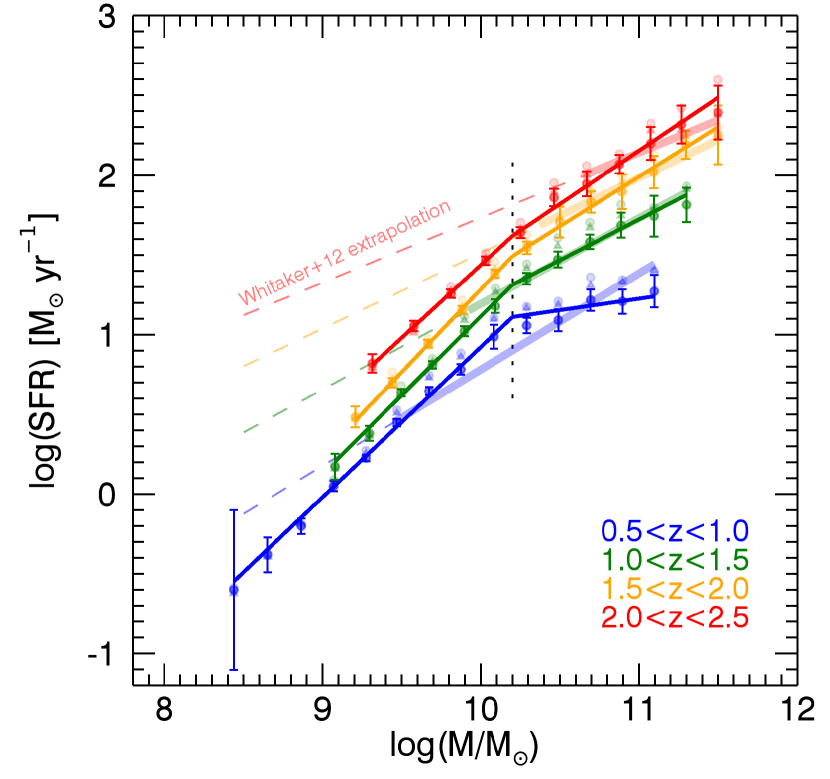
Figure 3.— The slope of the $\log\Psi-\log\mathrm{M_{\star}}$ relation is measured separately for star-forming galaxies more massive and less massive than $\log(\mathrm{M_{\star}/M_{\odot}})=10.2$, using the UV+IR SFRs derived through a stacking analysis. The lighter color symbols indicate average stacks, whereas the darker color signify median stacks. The triangles signify stacking analyses where AGN candidates are removed. We include the best-fit relations from Whitaker et al. (2012b) for comparison, where the lighter color thick lines represent complete samples and the dashed lines indicate extrapolations into parameter space with no data. The Whitaker et al. (2012b) relations are shifted down by 0.046 dex to account for the difference between the Chabrier (2003) and Kroupa (2001) IMFs.

Figure 4.— Evolution of the slope of the $\log\Psi-\log\mathrm{M_{\star}}$ relation. The slope is roughly constant with redshift at $\sim 1.0$ for low mass galaxies, where as we see strong evolution in the slope for more massive galaxies, evolving from $\sim 0.6$ at $z=2$ to $\sim 0.3$ at $z=1$. The open circles are measurements on the average stacks, whereas the filled circles represent median stacks. The triangles signify stacking analyses where AGN candidates are removed.

We fit the $\log\Psi-\log\mathrm{M_{\star}}$ relation with a broken power law, to independently quantify the behavior of the low mass galaxies and the high mass galaxies. Figure 3 shows the best-fit relations using the UV+IR SFRs derived in the stacking analysis with stellar masses corrected for emission line contamination. The broken power law is parameterized as,

$$\log\Psi=a\left[\log\left(\frac{\mathrm{M_{\star}}}{\mathrm{M_{\odot}}}\right)-10.2\right]+b,$$ (3)

where the value of $a$ is different above and below the characteristic mass of $\log(\mathrm{M_{\star}/M_{\odot}})=10.2$. If we instead allow the characteristic mass to vary, the best-fit value ranges from $\log(\mathrm{M_{\star}/M_{\odot}})=10.0\pm 0.1$ at $0.5<z<1.0$, to $\log(\mathrm{M_{\star}/M_{\odot}})=10.2\pm 0.1$ at $1.0<z<2.0$, up to $\log(\mathrm{M_{\star}/M_{\odot}})=10.5\pm 0.3$ at $2.0<z<2.5$. Fixing the characteristic mass to $\log(\mathrm{M_{\star}/M_{\odot}})=10.2$ does not significantly effect the measured redshift evolution of the slope. The best-fit coefficients are presented in Table 3. The slope measurements at the high-mass end are consistent with the NMBS data analysis (Whitaker et al., 2012b), shown in lighter colors for reference. However, we note that the slope evolution in Equation 2 of Whitaker et al. (2012b) does not formally agree due to the different stellar mass ranges considered in their linear fits (thick solid lines in Figure 3). The dashed lines in Figure 3 indicate extrapolations that enter parameter space where no data are available for NMBS.

We show the evolution of the measured slope for low mass ($\log(\mathrm{M_{\star}/M_{\odot}})<10.2$) and high mass ($\log(\mathrm{M_{\star}/M_{\odot}})>10.2$) galaxies in Figure 4. The data are consistent with no evolution in the slope for low mass galaxies, with an average measured value of $\alpha=0.97\pm 0.06$ (grey solid line)

On the other hand, we observe a strong evolution in the slope at the high mass end of the $\log\Psi-\log\mathrm{M_{\star}}$ relation. We measure a slope of $\alpha\sim 0.7$ at $z>2$, whereas the relation becomes shallower with time reaching a value of $\alpha\sim 0.3$ by $z\sim 1$. We fit the high-mass slopes as a function of redshift, finding a strong evolution in the slope for massive galaxies ($\log(\mathrm{M_{\star}/M_{\odot}})>10.2$), with the following best-fit relation:

$$\alpha(z)=0.03\pm 0.10+(0.31\pm 0.06)z.$$ (4)

To test if the changing slope of the star formation sequence could be partly a result of contamination due to AGN, we redo our stacking analyses after removing AGN candidates. Spitzer/IRAC selection is a powerful tool for identifying luminous AGNs. As all five CANDELS fields have uniform coverage with deep Spitzer/IRAC imaging, we remove all sources that fall within the revised IRAC color-color selections presented in Donley et al. (2012). The Donley et al. (2012) selection is more restrictive than the standard “wedge” (e.g., Stern et al., 2005), such that distant star-forming galaxies are not removed unnecessarily. The adopted AGN selection criteria is therefore optimized for the present dataset. We find that removing AGN candidates from the sample does not significantly change the measured slope of the star formation sequence. The change in SFR varies smoothly from an overestimate of order 0.02–0.06 mag at the lowest masses when not removing AGN candidates, to an underestimate of 0.08–0.1 mag at the highest masses. The results from the stacking analyses with AGN candidates removed are indicated by triangles in Figures 3 and 4. Although the average low-mass slope is higher with a measured value of $\alpha=1.06\pm 0.06$, both the low-mass and high-mass slopes agree within the formal error bars.

In this section we have quantified the behavior of the slope of the star formation sequence in different mass intervals. We find that on average, emission line contamination to the stellar masses cannot account for the different slopes of low and high masses, as detailed in Appendix A. Although we correct for emission line contamination, we have not accounted for contamination to the broadband fluxes due to the nebular continuum here. This effect is only significant where the fraction of nebular gas relative to stars is high, or $W_{\mathrm{H\alpha}}\gtrsim 300$ (e.g., Izotov et al., 2011). There may therefore be additional contamination of our stellar masses due to the nebular continuum for $\log(\mathrm{M_{\star}/M_{\odot}})<9.5$ at $z>2$. In practice, the lowest mass bin above our mass-completeness limits at $2.0<z<2.5$ may be slightly overestimated. In the next section, we explore the effects of the assumed calibrations to convert the observed 24$\mu$m flux density and the rest-frame 2800$\mathrm{\AA}$ luminosities into SFRs.

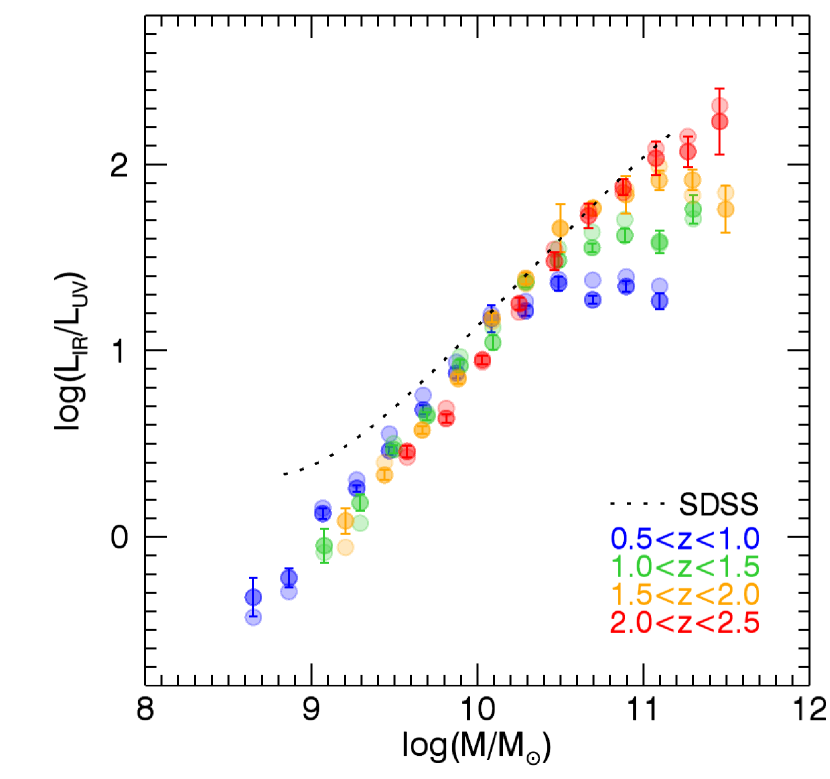
Figure 5.— The infrared excess ($\mathrm{IRX}\equiv\mathrm{L}_{\mathrm{IR}}$/L_UV) as a function of stellar mass for the median and average stacks, darker and lighter color symbols, respectively. More massive star-forming galaxies have higher $\log\mathrm{(L_{IR}/L_{UV})}$ ratios, suggesting increasing amounts of dust attenuation. There is surprisingly little evolution in the average $\log\mathrm{(L_{IR}/L_{UV})}$–$\log\mathrm{M_{\star}}$ relation at $\log(\mathrm{M_{\star}/M_{\odot}})<10.5$. There exists a trend at $\log(\mathrm{M_{\star}/M_{\odot}})>10.5$ for more dust per fixed stellar mass towards higher redshift, but we note that the relation itself has a relatively large intrinsic scatter. The dotted black line indicates the inferred $\log\mathrm{(L_{IR}/L_{UV})}$ ratios from Balmer decrement measurements with SDSS from Garn & Best (2010).

V. Uncertainties in Star Formation Rates

Here, we explore the uncertainties in the UV+IR star formation rates in greater detail. In particular, we explore the implications of the dependence of the rest-frame IR to UV bolometric luminosity ratios (Section V.1) and the gas-phase metallicity (Section V.2) on stellar mass.

V.1. Stellar Mass Dependence of L_IR/L_UV

We observe a curvature of the $\log\Psi-\log\mathrm{M_{\star}}$ relation towards lower sSFRs for the most massive star-forming galaxies. The implication is that the most massive star-forming galaxies have older stellar populations, as the inverse of the sSFR defines a timescale for the formation of the stellar population of a galaxy. However, the evolution measured for the mass dependency of the $\log\Psi-\log\mathrm{M_{\star}}$ relation in Figure 1 relies on a proper accounting of the dust content of the galaxies.

The infrared excess ($\mathrm{IRX}\equiv\mathrm{L}_{\mathrm{IR}}$/L_UV) probes the amount of dust in a galaxy, and has been shown to be a strong function of stellar mass (e.g., Reddy et al., 2006, 2010; Whitaker et al., 2012b). Figure 5 shows the IRX ratio as derived from the stacking analysis for the different stellar mass bins, including error bars from the bootstrap analysis. Although there is a large intrinsic scatter in this ratio (e.g., Whitaker et al., 2012b), we see remarkably little redshift evolution in the average ratio below $\log(\mathrm{M_{\star}/M_{\odot}})=10.5$.

To our knowledge, there does not exist a direct measurement of IRX as a function of stellar mass for local galaxies. The dotted black line in Figure 5 is derived from the Balmer decrement measurements from the SDSS sample presented in Garn & Best (2010). We assume the Calzetti et al. (2000) dust extinction law to convert the measured H$\alpha$ extinction to the extinction at 1600$\mathrm{\AA}$. Meurer et al. (1999) provide an empirical relation between A₁₆₀₀ and IRX₁₆₀₀. We note that we are measuring IRX_UV, as calculated from $1.5\nu\mathrm{L}_{\nu 2800}$, which should be roughly equivalent (Kennicutt, 1998). We find that the IRX ratio inferred from SDSS data is about 0.1 dex higher than the ratio we measure in this work at $\log\mathrm{M_{\star}}=9.5-11$ M_⊙. The offset of up to $\sim 0.5$ dex at $\log\mathrm{M_{\star}}\lesssim 9$ may result because the Garn & Best (2010) sample is selected on the basis of emission lines being detected, which could introduce selection biases. Although the overall offset of $\sim 0.1$ dex may be due to calibration uncertainties, it is more likely related to the assumed conversions to convert the direct SDSS Balmer decrement measurements to an inferred IRX ratio. In our data, we find no evolution with redshift from $z=0.5$ to $z=2.5$ for $\log(\mathrm{M_{\star}/M_{\odot}})<10.5$. There appears to be a trend for higher IRX ratios with increasing redshift for $\log(\mathrm{M_{\star}/M_{\odot}})>10.5$. However, the inferred SDSS IRX ratio is inconsistent with this evolution towards lower IRX ratios at higher masses. If there are systematic errors in our calibration of $\mathrm{L_{IR}}$ to a SFR, then the effect of this error will depend on mass. In particular, if the conversion from 24$\mu$m to $\mathrm{L_{IR}}$ underestimated the luminosity, it would introduce a trend similar to Figure 1.

V.2. Effect of Gas-Phase Metallicity on 24$\mu$m Flux Density

The gas-phase metallicities of galaxies are observed to be a strong function of their stellar mass (e.g., Tremonti et al., 2004; Erb et al., 2006; Mannucci et al., 2010; Zahid et al., 2011; Steidel et al., 2014), where less massive galaxies have fewer metals. This relation has several implications with respect to the calibration of SFR indicators over a broad range in stellar mass. The Spitzer/MIPS 24$\mu$m imaging captures strong aromatic emission features, thought to be due to polycyclic aromatic hydrocarbons (PAHs). PAH formation and destruction is sensitive to the metallicity of a galaxy; observations show a metallicity-dependence of the PAH abundance in galaxies (e.g., Engelbracht et al., 2005; Madden et al., 2006), with a paucity of PAH detection in low metallicity galaxies ($Z<0.1Z_{\odot}$; e.g., Hunt et al., 2010).

Although SFRs derived from Spitzer/MIPS 24$\mu$m imaging are in excellent agreement with Herschel measurements (Wuyts et al., 2011), this indicator is not well-calibrated in low mass galaxies. Furthermore, the fraction of IR light from dust heated by old stars remains poorly constrained, a problem that is likely most relevant in more massive galaxies (Kennicutt, 1998; Rieke et al., 2009). Taking the agreement with Herschel FIR measurements at face value, we only consider the former problem here; the reliability of SFRs extrapolated from the empirical Spitzer/MIPS 24$\mu$m calibration is unknown for low mass galaxies. Hunt et al. (2010) show that although the fraction of PAH emission normalized to the total IR luminosity is considerably smaller in metal-poor galaxies, they show signs of a harder radiation field through a deficit of small PAHs. The weaker PAH emission may be offset by the harder radiation field, conspiring to minimize potential mass-dependent systematic effects when using the rest-frame 6–14$\mu$m to infer the IR SFR (where we probe $\sim 7\mu$m at $z=2.5$ and just outside the PAH window at $\sim 16\mu$m for $z=0.5$). However, Engelbracht et al. (2005) observe an abrupt shift in the mean 8-to-24$\mu$m flux density ratio between 0.3 and $0.2Z_{\odot}$ due to a decrease in the 8$\mu$m flux density.

The paucity of PAH features is observed for metallicities less than 0.1–0.2$Z_{\odot}$. Zahid et al. (2011) and Erb et al. (2006) show that the average metallicity is also $>0.1Z_{\odot}$ at least above $\log(\mathrm{M_{\star}/M_{\odot}})$ of 9.2 and 9.5 at $z=0.8$ and $z>2$, respectively. Although the strength of the PAH features will depend on the metallicity, only our lowest mass bins could significantly suffer from 24$\mu$m luminosity to SFR calibration issues due to a complete lack of PAH features altogether. The steeper slope of the $\log\Psi-\log\mathrm{M_{\star}}$ relation is still observed at $\log(\mathrm{M_{\star}/M_{\odot}})=9.5-10$, so we suspect that the measurements presented in Figure 4 should therefore hold irrespective of unknown metallicity effects. Future studies of gravitationally lensed low-mass systems may shed light on this matter.

As we cannot formally account for the systematic uncertainties in the $\mathrm{SFR_{IR}}$ introduced at low stellar masses due to changing gas-phase metallicities, we instead derive SFRs that are independent of the 24$\mu$m to bolometric IR luminosity conversion in the following section. In the absence of FIR data, we can estimate the total SFR from the measured UV luminosity by assuming a correlation between the slope of the UV continuum and dust extinction, and from H$\alpha$ emission.

Figure 6.— The infrared excess ($\mathrm{IRX}\equiv\mathrm{L}_{\mathrm{IR}}$/L_UV) as a function of the slope of the UV continuum, where probe quantities probe the amount dust in a galaxy. High IRX ratios and shallower UV continuum slopes are indicative of higher dust extinction. The data is consistent with little evolution in the IRX-$\beta$ correlation at $1.0<z<2.5$, with an offset towards lower IRX ratios for our lowest redshift bin of $0.5<z<1.0$. We compare our self-consistent measurements of this correlation to various parameterizations presented in the literature. The lighter color symbols represent the ratio from average stacks, whereas the darker color symbols were measured from median stacks.

VI. Other Star Formation Indicators

Adding the rest-frame UV light of massive stars to that re-radiated at FIR wavelengths is considered the best practice to obtain reliable total SFRs (e.g., Speagle et al., 2014), but we can also consider alternative SFR indicators that do not suffer from the same calibration uncertainties at low stellar masses. With the 3D-HST photometric catalogs, we can derive total SFRs from L_UV with a $\beta$ dust correction, and also measure L_Hα (for a smaller redshift range where H$\alpha$ is covered by the WFC3/G141 grism).

VI.1. Dust corrections to the UV Continuum

The rest-frame UV spectrum is nearly flat in L_ν over the wavelength range of 1200–3000Å, which allows us to express the conversion from the observed 2800Å luminosity to the integrated UV luminosity in a relatively simple form (Kennicutt, 1998). This conversion implicitly assumes that galaxies continuously form stars over timescales of 100 Myr or longer. As we are probing the average SFR of galaxy populations as a whole, this assumption is probably justified. To test our assumption of solar metallicity, we compare spectra produced from the stellar synthesis code Starburst 99 (Leitherer et al., 1999; Vázquez & Leitherer, 2005; Leitherer et al., 2010). We find that the correction to the rest-frame 2800Å luminosity to account for the slope between 1216–3000Å increases by only 2% when instead assuming continuous star-formation over a 100 Myr with a Kroupa (2001) IMF and 0.4$Z_{\odot}$. A higher metallicity of 2$Z_{\odot}$ results in a slightly shallower UV continuum slope and a decrease in the correction to the rest-frame 2800Å luminosity by 7%. Thus, our calculation of the rest-frame UV luminosity does not strongly depend on our assumption of solar metallicity.

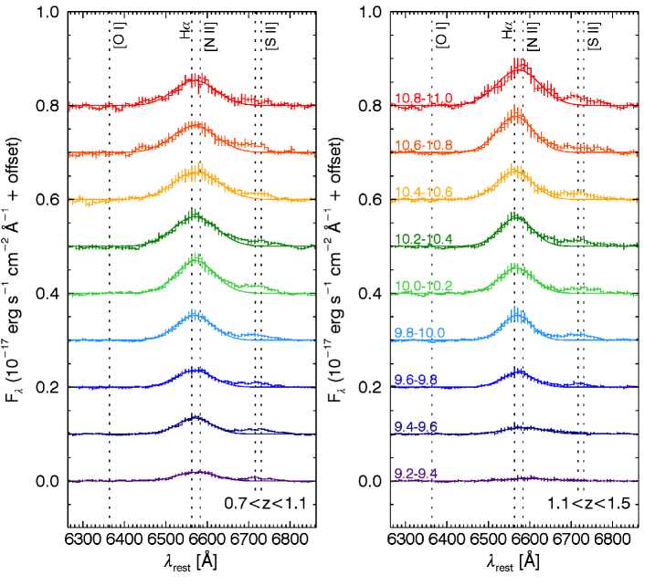
Figure 7.— H$\alpha$ stacks of HST/WFC3 G141 grism spectroscopy from the 3D-HST survey for all star-forming galaxies with coverage at $0.7<z<1.5$, split in two redshift bins and nine bins of stellar mass with 0.2 dex width. Where a grism redshift has not yet been calculated (for $H_{F140W}>23$), we adopt the photometric redshift. We measure the H$\alpha$ emission line fluxes to derive SFRs.

The use of the rest-frame UV continuum slope $\beta$ as a dust correction to L_UV remains largely uncertain with little consensus in the literature. Figure 6 shows correlation between IRX and $\beta$ from this work, compared to a range of best-fit relations from the literature. The Meurer et al. (1999) relation is derived from the UV spectra and fluxes of local starbursts and used to empirically calibrate the $\mathrm{L_{IR}/L_{UV}}$ correlation with $\beta$ in terms of the dust absorption at 1600$\mathrm{\AA}$. This only agrees well with our data at $z>1.5$ and $\beta>-0.5$, whereas the data are lower by 0.2–0.5 dex otherwise. It is difficult to say if the offset in the lowest redshift bin is intrinsic, as the rest-frame UV continuum is often sampled by only the two bluest photometric bands. The offset may also be due to systematic uncertainties in the 24$\mu$m to total bolometric IR luminosity calibration as discussed in Section V, or some other unknown calibration error.

Recent work by Takeuchi et al. (2012) finds a significantly lower $z=0$ relation for the same sample of local starburst galaxies as Meurer et al. (1999), when aperture corrections to the UV flux are properly taken into account. Our measurements of the IRX correlation with $\beta$ are identical to the Takeuchi et al. (2012) $z=0$ relation at $0.5<z<1.0$, and 0.1–0.4 dex higher at all other redshifts. Taken at face value, the dust properties of galaxies at $z>1$ may be different from local star-forming galaxies. Similarly, Oteo et al. (2014) find that the IRX-$\beta$ relations for local starbursts are insufficient at high redshifts to recover the necessary dust-correction factors to reconcile the observed FIR with the derived SFR. They suggest an evolution of the dust properties of star-forming galaxies with redshift. We do not find evidence for a strong evolution in the average dust properties of galaxies at $0.5<z<2.5$, although galaxies at $z>1$ do appear to have different dust properties than local starburst galaxies (see also, e.g., Kashino et al., 2013; Price et al., 2014). The strong redshift evolution observed by Oteo et al. (2014) may be a result of their sample selection.

In another high redshift study, Heinis et al. (2013) perform a stacking analysis of a sample of UV-selected galaxies at $z\sim 1.5$ and find a correlation that underestimates the correlation derived from local starburst galaxies but is in good agreement with that derived from local normal star-forming galaxies. The correlation we measure at $z\sim 1.5$ generally agrees with the Heinis et al. (2013) relation. Galaxies at $z\sim 1.5$ may therefore be more similar in their dust properties to “normal” local galaxies rather than starburst galaxies. From Figure 6, we see that there is little consensus amongst the measured correlations in the literature. The relations presented in the literature show a larger scatter than the self-consistent measurements presented herein.

Figure 8.— Comparison of the star formation sequence as measured with UV+IR SFRs (shown in transparency), relative to other SFR indicators independent of the FIR: H$\alpha$ SFRs (diamonds) and UV luminosities corrected by the slope $\beta$ of the UV continuum. The slope measured at low stellar masses is consistent amongst the 3 independent SFR indicators with a constant value of order $\alpha\sim 0.8-1$ from $z=0.5$ to $z=2.5$.

To estimate the total SFR from the UV alone, we correct $\mathrm{L_{UV}}$ for each bin in stellar mass by the average measured UV continuum slope, $\mathrm{L_{2800,corr}}=\mathrm{L}_{2800}\times 10^{0.4A_{2800}}$. We use the Meurer et al. (1999) relation, $\mathrm{A_{1600}}=4.43+1.99\beta$, and the Calzetti et al. (2000) dust law to convert $\mathrm{A_{1600}}$ to $\mathrm{A_{2800}}$. We only consider stellar mass bins where $\beta<-0.5$, as Wuyts et al. (2011) show that dust-corrected SFR measurements above these limits become highly uncertain because the majority of the rest-frame UV light is absorbed (see also Figures 5 and 6 here). In practice, this limits us to low stellar masses where galaxies have less dust. We discuss these measurements of the $\log\Psi-\log\mathrm{M_{\star}}$ relation in the following section, together with H$\alpha$ SFRs.

VI.2. H$\alpha$ Star Formation Rates

The main uncertainty when inferring the total SFRs without FIR data remains the dust correction, which becomes increasingly significant at shorter wavelengths. Although the dust correction at 6500$\mathrm{\AA}$ is still significant, H$\alpha$ is less affected by dust than the UV continuum. The 3D-HST G141 grism spectroscopy covers the H$\alpha$ emission line at $0.7<z<1.5$. We therefore select all galaxies in this redshift range with 3D-HST coverage (which includes roughly $\sim 75\%$ of the CANDELS $J_{F125W}$ and $H_{F160W}$ imaging) and perform a stacking analysis to measure H$\alpha$ line fluxes. Grism redshifts and emission line fluxes are only measured down to $H_{F160W}=23$ mag for the 3D-HST v4.0 internal release, whereas the one dimensional (1D) spectra are extracted for all objects. We select galaxies with a S/N ratio greater than 10 in the $H_{F140W}$ direct image for two redshift bins at $0.7<z<1.1$ and $1.1<z<1.5$ and split the sample into the same 0.2 dex stellar mass bins as the UV+IR analysis, using the photometric redshift where a grism redshift is not available for $H_{F160W}>23$.

The 1D spectra are scaled to match the well-calibrated HST/WFC3 photometry by taking the ratio of $H_{F140W}$ to the average continuum flux in the G141 spectrum. We shift the spectra to the rest-frame and interpolate to a wavelength grid with $\Delta\lambda=8\mathrm{\AA}$. We fit a second order polynomial to the individual spectra, masking out the H$\alpha$ emission line, to parameterize and subtract the continuum. For each stellar mass, we measure a median and average rest-frame spectrum from the stacks. We show the average H$\alpha$ stacks in Figure 7. In addition to H$\alpha$, we clearly detect the [SII] emission lines. The S/N ratio in the G141 spectra becomes too below $\log(\mathrm{M_{\star}/M_{\odot}})=9.2$ to make robust H$\alpha$ emission line flux measurements. The lower photometric redshift accuracy will act to broaden the emission lines, but not to the degree where we expect H$\alpha$ to blend with [SII]. The error bars presented in Figure 7 are derived from 50 iterations of a bootstrap analysis.

Both the mean and median spectra are fit with a Gaussian (solid lines in Figure 7), from which we measure the H$\alpha$ emission line fluxes. Following Wuyts et al. (2013), we assume that [NII] contributes 15% of the measured H$\alpha$ emission line flux such that the [NII]/(H$\alpha$+[NII]) ratio equals 0.15. The SFR is derived from the H$\alpha$ flux using the conversion presented in Kennicutt (1998), adapted from a Salpeter IMF to a Chabrier (2003) IMF following (Muzzin et al., 2010):

$$\Psi_{\mathrm{H\alpha}}~{}[\mathrm{M_{\odot}~{}yr^{-1}}]=1.7\times 10^{-8}~{}\mathrm{L_{H\alpha}}~{}[\mathrm{L_{\odot}}].$$ (5)

The measured H$\alpha$ SFRs are presented together with the SFRs derived from the $\beta$-corrected $\mathrm{L_{UV}}$ in Figure 8. Filled circles and diamonds signify the UV+$\beta$-correction SFRs and the H$\alpha$ SFRs derived from the mean stacks, respectively, whereas the open diamonds correspond to the measurements from median stacks. The $\beta$-corrected UV SFRs agree within 0.1 dex with the UV+IR SFRs at $\log\mathrm{M_{\star}}=10$ M_⊙, but become increasingly higher by up to $\sim 0.2$ dex at $\log\mathrm{M_{\star}}=9$ M_⊙. We suspect these offsets are related to the large uncertainties in the conversion from $\beta$ to $A_{1600}$. The H$\alpha$ SFRs are offset by $\sim 0.5$ dex from the UV+IR SFRs, presumably because they do not include a dust correction. This offset implies $\sim 1.3$ magnitudes of extinction in H$\alpha$ for $\log(\mathrm{M_{\star}/M_{\odot}})<10.2$. This value is larger than the estimates of Garn et al. (2010) that range from $\mathrm{A_{H\alpha}}=0.3-1$ at $\log\mathrm{M_{\star}}\sim 9-10$ M_⊙. Although stacks of emission-line detected galaxies with grism redshifts are consistent with the running mean of the individual measurements, we cannot rule out uncertainties in our analysis introduced due to our use of photometric redshifts for the larger (lower-mass) sample. Above $\log(\mathrm{M_{\star}/M_{\odot}})=10.2$, the H$\alpha$ SFRs are almost flat, which we interpret as due to the large dust corrections necessary at the massive end. Due to the strong correlation between the amount of dust in a galaxy (as probed through the IRX ratio) and the stellar mass, dust corrections will only act to steepen the derived $\log\Psi-\log\mathrm{M_{\star}}$ relation. The slope we measure from the H$\alpha$ SFRs for $\log(\mathrm{M_{\star}/M_{\odot}})<10.2$ therefore acts as a lower limit, independent of the other SFR indicators explored in this paper.

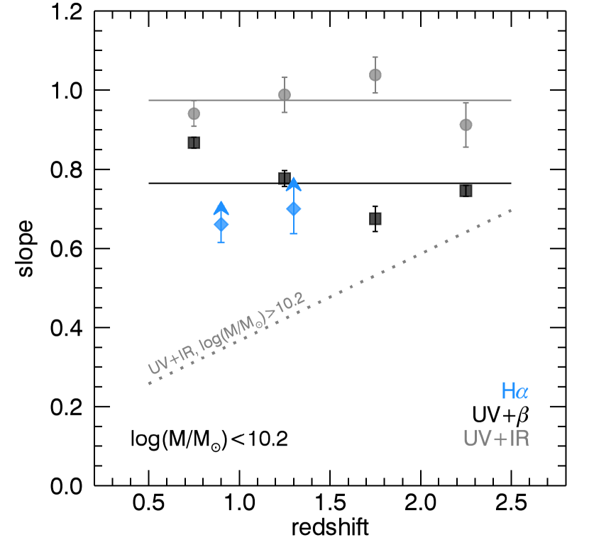
Figure 9.— Evolution of the low mass slope ($\log\mathrm{M_{\star}}<10.2$ M_⊙) with redshift for SFR indicators independent of the IR. The low mass slope of the $\log\Psi-\log\mathrm{M_{\star}}$ relation is roughly constant from $z=0.5$ to $z=2.5$, as measured from 3 independent SFR indicators. The H$\alpha$ SFRs do not include any dust correction and therefore serve as lower limits to the slope due to the strong correlation between the amount of dust in a galaxy and its stellar mass. The solid horizontal lines represent the average measured low mass slopes for the different SFR indicators.

Figure 10.— Evolution of the sSFR with redshift in bins of stellar mass. The sSFR exhibits a mass-dependent redshift evolution in both the UV+IR SFRs (left) and the $\beta$-corrected UV SFRs (right). Whereas the sSFRs of the most massive galaxies evolve strongly with redshift, all galaxies less massive than $\log(\mathrm{M_{\star}/M_{\odot}})=10$ show roughly the same shallower redshift evolution. The $\beta$-corrected UV SFRs exhibit a slightly shallower redshift evolution than the UV+IR SFRs, however large uncertainties remain in the $\beta$ calibration.

We compile the measurements of the slope of the $\log\Psi-\log\mathrm{M_{\star}}$ relation below $\log(\mathrm{M_{\star}/M_{\odot}})=10.2$ in Figure 9. Both the UV continuum and H$\alpha$ measurements are consistent with a steeper slope for low mass galaxies at all redshifts. Both the UV+IR and UV continuum low-mass slopes are constant with redshift, but systematically offset by 0.2. These differences may be due to the large uncertainties remaining in the $\beta$-$A_{1600}$ calibration, as evident from Figure 6.

VII. Evolution in the Specific Star Formation Rate

The mass-dependent time evolution of the sSFR is presented in Figure 10 for the UV+IR SFRs (left panel) and the SFRs derived from the $\beta$-corrected UV luminosity (right panel). Following previous studies in the literature (e.g., Damen et al., 2009), we parameterize the redshift evolution of the sSFR as,

$$\frac{\Psi}{\mathrm{M_{\star}}}~{}[\mathrm{yr^{-1}}]=a(1+z)^{b}.$$ (6)

We present the best-fit values for both the UV+IR and $\beta$-corrected UV sSFRs in Table 4. We observe a mass-dependent redshift evolution in both SFR indicators, where galaxies less massive than $\log(\mathrm{M_{\star}/M_{\odot}})=10$ exhibit a similar evolution with $b=1.9$ for UV+IR SFRs and a slightly lower average value of $b=1.8$ for $\beta$-corrected UV SFRs. Galaxies more massive than $\log(\mathrm{M_{\star}/M_{\odot}})=10$ show a stronger redshift evolution, reaching a maximum value of $b=3.5$ for $\log(\mathrm{M_{\star}/M_{\odot}})>11$. As discussed in Section VI.1, shallow UV continuum slopes are not well-calibrated and we therefore cannot accurately measure the redshift evolution from the $\beta$-corrected UV SFRs for galaxies more massive than $\log(\mathrm{M_{\star}/M_{\odot}})=10.5$.

A plausible explanation for the decline in the sSFR since $z\sim 2$ is a decrease in the gas accretion rate on to galaxies (e.g., Dutton et al., 2010). The specific accretion rate for dark matter haloes scales as $(1+z)^{2.25}$ for $z<2$ (Birnboim et al., 2007), similar to the average evolution in the sSFR for low-mass galaxies. Semi-analytic models (SAMs) predict a similar evolution with $b=2.5$ (Guo et al., 2011), whereas the observed redshift evolution from previous studies is larger with $b\sim 3-5$ (e.g., Salim et al., 2007; Damen et al., 2009; Karim et al., 2011), and only marginally consistent with the evolution we measure for the most massive galaxies. The redshift evolution we measure for low mass galaxies agrees to first order with the theoretical predictions, whereas the more rapid evolution for massive galaxies remains discrepant with models. This discrepancy likely relates to the poorly understood physics of the quenching of star-formation.

Table 4Evolution of the specific star formation rate

	UV+IR		UV+$\beta$
$\log(\mathrm{M_{\star}/M_{\odot}})$	$\log a$	$b$	$\log a$	$b$
9.2–9.4	$-9.54\pm 0.15$	$1.95\pm 0.24$	$-9.47\pm 0.23$	$2.10\pm 0.37$
9.4–9.6	$-9.50\pm 0.14$	$1.86\pm 0.22$	$-9.39\pm 0.23$	$1.78\pm 0.37$
9.6–9.8	$-9.54\pm 0.07$	$1.90\pm 0.12$	$-9.43\pm 0.30$	$1.77\pm 0.48$
9.8–10.0	$-9.58\pm 0.03$	$1.98\pm 0.04$	$-9.46\pm 0.34$	$1.70\pm 0.54$
10.0–10.2	$-9.69\pm 0.03$	$2.16\pm 0.04$	$-9.45\pm 0.37$	$1.43\pm 0.59$
10.2–10.4	$-9.93\pm 0.08$	$2.63\pm 0.12$	$-9.99\pm 0.34$	$2.31\pm 0.52$
10.4–10.6	$-10.11\pm 0.10$	$2.88\pm 0.16$	$-9.72\pm 0.29$	$1.52\pm 0.43$
10.6–10.8	$-10.28\pm 0.15$	$3.03\pm 0.24$	–	–
10.8–11.0	$-10.53\pm 0.17$	$3.37\pm 0.26$	–	–
11.0–11.2	$-10.65\pm 0.11$	$3.45\pm 0.17$	–	–

• Notes. Redshift evolution of the sSFR is parameterized in Equation 6. We include the redshift evolution as measured from the UV+IR SFR indicator and the $\beta$-corrected UV SFR. The $\beta$-corrected UV SFR is unreliable at the highest stellar masses and we therefore only include measurements for $\beta<-0.5$.

VIII. Broader Implications

In this paper, we present an empirical study of the properties of the star formation sequence over roughly half of cosmic time ($0.5<z<2.5$). The three main observable quantities of the star formation relation, the normalization, intrinsic scatter, and slope, encapsulate fundamental physical quantities that regulate star formation. The normalization of the star formation sequence is governed predominantly by the changing cosmological gas accretion rates with redshift. The intrinsic scatter of this relation reveals the level of stochasticity in the gas accretion history. Lastly, the measured slope of this relation tells about star formation efficiency. As the various different feedback mechanisms are known to dominate at different stellar mass regimes, it should perhaps come as no surprise that we now measure for the first time different slope and normalization evolution for low and high mass galaxies.

We measure the slope of the star formation sequence for complete samples of both low mass and high mass galaxies at $0.5<z<2.5$, finding a steeper slope for less massive galaxies. From a radio stacking analysis, Karim et al. (2011) found tentative evidence for curvature of the star formation sequence. However, they only considered blue star-forming galaxies and all the deviations occurred below the mass representativeness limits, so no conclusions could be reached. Similarly, Whitaker et al. (2012b) explored the changing slope of the star formation sequence in greater detail at $z\sim 1$, finding that the bluest (lowest mass) galaxies had a steeper slope than redder (high mass) galaxies. As the color of a galaxy is directly correlated with the amount of dust, these observations demonstrate why measurements of the slope from UV SFRs are often closer to unity ($\alpha\sim 0.75-1$), whereas IR SFRs are shallower with a slope of $\alpha\sim 0.6$ (Speagle et al., 2014). Here, we present the first statistically robust measurement of the low-mass slope of the star formation sequence using UV+IR SFRs for mass-complete samples at $0.5<z<2.5$.

We observe that the star formation sequence has a roughly constant slope of $\alpha\sim 1$ for $\log(\mathrm{M_{\star}/M_{\odot}})<10.2$. Dust-corrected H$\alpha$ measurements of the star formation sequence for both star-forming and quiescent galaxies in the SDSS by Brinchmann et al. (2004) result in a slightly shallower slope of $\alpha=0.7$, with a drop in SFR beyond $\log(\mathrm{M_{\star}/M_{\odot}})=10$. Local studies by Huang et al. (2012) suggest a transition mass of $\log(\mathrm{M_{\star}/M_{\odot}})\sim 9.5$ below which star formation scales differently with total stellar mass (also found by Salim et al., 2007; Gilbank et al., 2011), with a steeper slope. Kannappan et al. (2009) identify a similar threshold stellar mass below which the number of blue sequence galaxies with elliptical morphologies sharply rises.

Many theoretical models predict a steep relation between $\log\mathrm{M_{\star}}$ and $\log\Psi$, but have trouble producing the shallow slope found for the massive star-forming galaxies (e.g., Somerville et al., 2008). The fact that we find a steep slope for the low-mass galaxies will make it easier to reconcile the galaxy formation models with the observations. The simple equilibrium models from Davé et al. (2012) are a notable exception, they actually predict a rather shallow slope at all masses, inconsistent with the results obtained here. Figure 11 presents a comparison between the momentum-driven wind models of the Davé et al. (2012) analytical framework, as outlined in detail in Section 7.1 of Henry et al. (2013a), and UV+IR SFRs measured from stacks of all galaxies (see Appendix C). Other studies favor these simple models because they produce the best-fit to a variety of quasar absorption line studies of the intergalactic medium, while also reproducing the observed cosmic star formation history (e.g., Oppenheimer & Davé, 2006, 2008). There are two possible explanations for the differences between the predictions from the equilibrium model of Davé et al. (2012) and other models. It could either be that the low-mass systems are not in equilibrium, as implicitly assumed in the Davé et al. (2012) framework, and the time-dependence of feedback must be properly quantified. Or it may be that the wind-recycling in these low-mass systems has been underestimated (e.g., Oppenheimer et al., 2010). Qualitatively, non-equilibrium models match the observed mass and redshift evolution of the SFR (e.g., Guo et al., 2013; Mitchell et al., 2014; Behroozi & Silk, 2014; Genel et al., 2014, see also summary in Figure 9 of Leja et al. 2014). Future detailed comparisons between the observed properties of the star formation sequence and models may place tighter constraints on the various feedback processes that galaxies undergo.

Figure 11.— Comparison between the UV+IR SFRs derived from a MIPS/24$\mu$m stacking analysis of all galaxies and predictions from the Davé et al. (2012) analytical equilibrium models, assuming momentum-driven winds and a quenching mass of $\log(\mathrm{M_{halo}/M_{\odot}})=12.3$. The UV+IR SFRs from the average (light open circles) and median (light filled circles) stacking analyses for star-forming galaxies only are shown for reference. These simple equilibrium models fail to match the steep slope at low masses, as well as the overall normalization, suggesting either non-equilibrium conditions or a departure from self-similar prescriptions for feedback.

In a recent paper, Leja et al. (2014) examine the connection between the observed correlation between $\log\Psi$ and $\log\mathrm{M_{\star}}$ from Whitaker et al. (2012b) and the observed stellar mass functions from Tomczak et al. (2014) at $0.2<z<2.5$. They find that an extrapolation of the relatively shallow slopes measured by Whitaker et al. (2012b) cannot hold true at the low-mass end, as this results in an extremely rapid growth of the stellar mass function at low stellar masses that is not observed. With a completely independent analysis, we show here that the slope for less massive galaxies is steeper than that measured for more massive galaxies. The mass function analysis by Leja et al. (2014) predicts a low-mass slope of $\alpha=0.9-1.1$, in agreement with the UV+IR SFRs, but slightly steeper than the $\beta$-corrected UV SFRs. Leja et al. (2014) note that some discrepancies between the stellar mass function and star formation sequence remain, even after adopting a low-mass slope of unity. For example, the normalization of the SFRs is $\sim 0.3$ dex higher than predicted from the growth of the mass function at $1<z<2.5$ (Leja et al. 2014; see also Genel et al., 2014).

We find a strong evolution in the slope of the star formation sequence for galaxies more massive than $\log(\mathrm{M_{\star}/M_{\odot}})>10.2$. This redshift evolution in the high-mass slope, combined with the redshift-dependent low-mass limit of the NMBS analysis, is likely what drove the evolution of the derived slope in Whitaker et al. (2012b). This strong evolution may be related to the growth of the bulge. Abramson et al. (2014) find that when accounting for the bulge/disk decomposition, the SFR renormalized by the disk stellar mass reduces the stellar mass dependence of star formation efficiency by $\sim 0.25$ dex per dex, reducing the slope by 0.25. Here we find that the difference between the slope for low-mass galaxies and high-mass galaxies increases from $\Delta\alpha=0.3$ at $z\sim 2$ to $\Delta\alpha=0.7$ at $z\sim 0.7$. Indeed, Nelson et al. (2012) find evidence for the rapid formation of compact bulges and large disks at $z\sim 1$. Similarly, Lang et al. (2014) observe that the bulge to disk ratio increases by a factor of two from $\log(\mathrm{M_{\star}/M_{\odot}})=10$ to $\log(\mathrm{M_{\star}/M_{\odot}})=11.5$. However, if the evolution of the high-mass slope is driven entirely by the growing contribution from the bulge to the stellar mass, Lang et al. (2014) should have also measured redshift evolution in the correlation between the bulge-to-disk and stellar mass. The average bulge-to-disk ratio is consistent between their two redshift bins at $z\sim 1$ and $z\sim 2$. We further caution that the formation of today’s bulge-disk systems was a complex process; in particular, galaxies with the present-day mass of the Milky Way increased their mass in the central regions at only a slightly smaller rate than at $r>2$ kpc (e.g., van Dokkum et al., 2013; Patel et al., 2013). Furthermore, as galaxies grow in mass, the sSFRs of individual galaxies likely evolved in a different way than the mean sSFR at fixed mass (e.g., Fumagalli et al., 2012; Leja et al., 2013). The idea that the shallower slopes measured for more massive galaxies is telling us about the growth of bulges in galaxies is intriguing, but warrants further analysis.

In Figure 12, we present the mass-doubling timescale. The inverse of the sSFR of a galaxy is often interpreted as a physical timescale for the formation of the stellar population, where $(\Psi/\mathrm{M_{\star}})^{-1}$ is equivalent to the time it would take for the stellar mass of a galaxy to double. We include both the median and average stacks in Figure 12, as denoted by the darker and lighter colors, respectively. The mass-doubling timescale is roughly self-similar for low-mass galaxies, evolving towards shorter formation timescales at earlier times. Whereas galaxies at $z\sim 0.5$ will double their mass in about a gigayear, this timescale is only 300 Myr at $z\sim 2$. This stellar mass doubling timescale implies high gas accretion rates at earlier times. The observed trends in the timescale for a galaxy to double in mass sets interesting constraints on feedback prescriptions in future efforts for galaxy formation theories.

Figure 12.— The mass-doubling timescale (sSFR^-1) as a function of stellar mass for star-forming galaxies. The filled circles with lighter colors represent the average stacks, whereas the darker circles represent median stacks. The highest stellar mass galaxies at a given epoch exhibit the longest mass-doubling timescales, whereas this timescale increases towards lower redshifts at fixed stellar mass. The mass-doubling timescale of low-mass galaxies evolves in a roughly self-similar fashion.

Here, we explore the average properties of the star formation sequence a factor of ten lower in stellar mass than previous studies for a single SFR indicator. With this unique dataset, we are therefore able to study the mass-dependencies of the normalization in addition to the slope. Previous studies of the redshift evolution of the sSFR (sensitive to the normalization of the star formation sequence) find results similar to our measurements for the most massive galaxies (e.g. Salim et al., 2007; Karim et al., 2011), with $\Psi/\mathrm{M_{\star}}\propto(1+z)^{3-4}$. We demonstrate in this paper that less massive galaxies exhibit a more gradual redshift evolution of their sSFRs, similar to the evolution of the cosmological gas accretion rate. We observe the redshift evolution in the sSFR to be self-similar for galaxies less massive than $\log(\mathrm{M_{\star}/M_{\odot}})=10$ with $\Psi/\mathrm{M_{\star}}\propto(1+z)^{1.9}$, whereas more massive galaxies show a stronger redshift evolution with $\Psi/\mathrm{M_{\star}}\propto(1+z)^{2.2-3.5}$ for $\log(\mathrm{M_{\star}/M_{\odot}})=10.2-11.2$. The redshift evolution for less massive galaxies is slightly shallower when using total SFRs derived from rest-frame UV luminosities corrected for dust by measuring the UV continuum shape. To our knowledge, such shallow redshift evolution in the sSFRs of galaxies has not been observed previously. Although Sobral et al. (2014) don’t see this strong mass dependence, their H$\alpha$ SFR measurements are highly dependent on the dust correction and their sample is not mass-selected. On the other hand, Behroozi et al. (2013) do find a similarly strong mass-dependence for the redshift evolution of the sSFR by connecting galaxies across all different epochs via abundance matching to halos in dark matter simulations. Similarly, although the absolute normalization is offset, the trend for galaxies less massive than $\log(\mathrm{M_{\star}/M_{\odot}})=10$ to show similar redshift evolution in their sSFRs qualitatively agrees with recent results from cosmological hydrodynamical simulations (Genel et al., 2014).

IX. Conclusions

In this paper, we combine the deep photometry available in the CANDELS legacy fields with the grism redshifts and H$\alpha$ emission line measurements from the 3D-HST treasury program, together with Spitzer/MIPS 24$\mu$m imaging. This unique combination of data allows us to leverage the strengths of each respective survey and enables significant improvements to our understanding of the star formation sequence relation across the full dynamic range in stellar masses over roughly half of cosmic history. With a mass-complete sample of 39,106 star-forming galaxies (out of a total sample of 58,973 star-forming galaxies) selected from the public 3D-HST photometric catalogs, we provide the average measured UV+IR SFRs from $z=0.5$ to $z=2.5$. For the first time, we firmly distinguish between distinct high and low mass slopes. The main results of our analysis are:

• We find that low-mass galaxies with $\log(\mathrm{M_{\star}/M_{\odot}})<10.2$ evolve in a self-similar fashion with a constant slope of unity ($\log\mathrm{\Psi}\propto\log\mathrm{M_{\star}}$), whereas we observe a strong evolution in the slope for more massive galaxies ranging from $\log\mathrm{\Psi}\propto(0.3-0.6)\log\mathrm{M_{\star}}$ from $z=0.5$ to $z=2$.

• We compare the total UV+IR SFRs, calibrated from a stacking analysis of Spitzer/MIPS 24$\mu$m imaging, to $\beta$-corrected UV SFRs and H$\alpha$ SFRs, finding that the low-mass slopes are consistently steeper than the high-mass slopes.

• We confirm previous studies, showing that the average IRX ratio ($\mathrm{L_{IR}/L_{UV}}$, a proxy for the amount of dust in a galaxy) is strongly correlated with stellar mass. For the first time, we show that this average relation is consistent with no redshift evolution from $z=0.5$ to $z=2.5$ for $9.0<\log\mathrm{M_{\star}}<10.5$ M_⊙.

• The redshift evolution of the normalization varies in different mass regimes. For galaxies less massive than $\log(\mathrm{M_{\star}/M_{\odot}})<10$ the specific SFR ($\Psi/\mathrm{M_{\star}}$) is observed to be self-similar with $\Psi/\mathrm{M_{\star}}\propto(1+z)^{1.9}$. More massive galaxies show a stronger evolution with $\Psi/\mathrm{M_{\star}}\propto(1+z)^{2.2-3.5}$ for $\log(\mathrm{M_{\star}/M_{\odot}})=10.2-11.2$.

Despite the many potential systematic uncertainties that remain in different SFR indicators, there appears to be a consensus forming with regards to the redshift evolution and mass dependencies of star formation. It would be valuable to analyze longer wavelength imaging to estimate mid-IR fluxes for the present dataset; our current analysis is limited to 24$\mu$m. We note that Rodighiero et al. (2014) analyzed Herschel 160$\mu$m imaging, and found that the star formation rates estimated from stacks agreed well between star formation rates from 160$\mu$m, 24$\mu$m, and dust-corrected UV luminosities. Exploration of the properties for the lowest mass galaxies beyond those presented in this paper is rich with potential for shaping our understanding of galaxy formation and evolution.

Appendix A Emission Line Corrections to Photometry and Stellar Masses

Figure 13.— Observed $\mathrm{H\alpha+N[II]}$ rest-frame equivalent widths of individual galaxies from the 3D-HST survey (circles) at $0.7<z<1.5$ are a strong function of stellar mass. We combine the linear best-fits (dashed lines) to the running means (diamonds) in two redshift bins with the redshift evolution from Fumagalli et al. (2012) of $W\propto(1+z)^{1.8}$ to derive $W(z,\mathrm{M_{\star}})$ in Equation A1.

Figure 14.— The contamination to stellar mass estimates as a function of stellar mass and redshift. The typical contamination from emission line flux to the broadband and medium-band photometry becomes important only for lower mass galaxies with $\log(\mathrm{M_{\star}/M_{\odot}})<9$, with the strongest trends observed at $2.0<z<2.5$. We compare the original stellar masses to those derived from the same stellar population synthesis modeling assumptions but including an additional subtraction of the contaminating emission line flux in the relevant photometric bands. On average, the stellar masses agree within $<0.04$ dex down to $\log(\mathrm{M_{\star}/M_{\odot}})=9.5$.

To estimate the direct effect of the contamination from emission line flux to the estimated stellar masses, we empirically derive the average correlation between the $\mathrm{H\alpha+N[II]}$ equivalent width ($W$) and stellar mass from individual 3D-HST line flux measurements in two redshift bins, $\mathrm{0.7<z_{grism}<1.1}$ and $\mathrm{1.1<z_{grism}<1.5}$ in Figure 13. At the HST/WFC3 grism resolution, the H$\alpha$ line is blended with [NII]. For the purposes of determining the emission-line contamination, it is not necessary to deblend these lines. To account for the redshift evolution of the $W-\log\mathrm{M_{\star}}$ relation we adopt the slope from the best-fit relation calculated by Fumagalli et al. (2012) of $W_{\mathrm{{H\alpha}}}\propto(1+z)^{p}$, where $p=1.8$. We note that we are extrapolating the measurements by Fumagalli et al. (2012) to lower stellar masses. Combining the redshift evolution from Fumagalli et al. (2012) with the $\log W_{\mathrm{{H\alpha+[NII]}}}-\log\mathrm{M_{\star}}$ relation we measure in Figure 13, we parameterize the redshift and mass dependence of the rest-frame H$\alpha$+[NII] $W$ as,

$$\log W_{\mathrm{{H\alpha}+[NII]}}=1.8\log(1+z)-0.32\left(\frac{\log\mathrm{M_{\star}/M_{\odot}}}{10^{10}}\right).$$ (A1)

In addition to the H$\alpha$+[NII] emission line flux contamination, we also estimate the contribution from the [OII]$\lambda$3727, 3729$\mathrm{\AA}$ and [OIII]$\lambda$4959,5007$\mathrm{\AA}$ doublets and H$\beta$. From the individual 3D-HST line flux measurements, we calculate an average $\log(F_{\mathrm{[OIII]}}/F_{\mathrm{H\beta}})$ value of $0.49\pm 0.04$ at $\log(\mathrm{M_{\star}/M_{\odot}})=10.2$ and $0.43\pm 0.05$ at $\log(\mathrm{M_{\star}/M_{\odot}})=10.8$. We combine these measurements with the low-mass stacking analysis of Henry et al. (2013b), who measure the $\log(F_{\mathrm{[OIII]}}/F_{\mathrm{H\beta}})$ ratio at $\log(\mathrm{M_{\star}/M_{\odot}})=8.2-9.8$. As we do not reach the same stellar mass limits as Henry et al. (2013b) and the line ratios may behave differently below $\log(\mathrm{M_{\star}/M_{\odot}})<8.5$, we ignore their lowest mass bin here. We find that $\log(F_{\mathrm{[OIII]}}/F_{\mathrm{H\beta}})$ has a weak mass dependence, which we use to derive the following correlation between the average ratio of the [OIII] to H$\alpha$+[NII] $W$ and stellar mass:

$$\frac{W_{\mathrm{{[OIII]}}}}{W_{\mathrm{{H\alpha+[NII]}}}}=0.95-0.46\left(\frac{\log\mathrm{M_{\star}/M_{\odot}}}{10^{10}}\right).$$ (A2)

To convert the observed $\log(F_{\mathrm{[OIII]}}/F_{\mathrm{H\beta}})$ ratios from H$\beta$ to H$\alpha$, we have assumed the most conservative case of a dust correction for case B recombination where $F_{\mathrm{{H\alpha}}}=2.86F_{\mathrm{H\beta}}$. When extrapolating the $W$ ratio from the emission line flux ratio, we must additionally make assumptions about the average continuum flux near [OIII] and H$\alpha$ as $W_{\mathrm{{[OIII]}}}/W_{\mathrm{{H\alpha}}}=F_{\lambda\mathrm{[OIII]}}/F_{\lambda\mathrm{H\alpha}}\times F^{c}_{\lambda\mathrm{H\alpha}}/F^{c}_{\lambda\mathrm{[OIII]}}$. We select galaxies at $z\sim 1.4$ where H$\alpha$ falls cleanly into the $H_{F160W}$ broadband filter and [OIII] in the $J_{F125W}$ broadband filter, finding an average $J_{F125W}-H_{F160W}$ color of -0.36 ABmag. Although the argument quickly becomes circular with emission-line contamination in the broadband filters, the contribution is expected to be small enough due to the broad filter width such that the average ratio can be used as a proxy for ${F^{c}_{\lambda\mathrm{H\alpha}}}/{F^{c}_{\lambda\mathrm{[OIII]}}}$ and folded into the constants in Equation A2. The $W_{\mathrm{[OIII]}}$ is equal to the $W_{\mathrm{H\alpha+[NII]}}$ at $\log(\mathrm{M_{\star}/M_{\odot}})\sim 10$, with lower values for more massive galaxies and higher values for less massive galaxies. As H$\beta$ falls in the same broadband filter as [OIII], we adopt the same correction for the continuum flux ratio to convert from the $W_{\mathrm{H\alpha+[NII]}}$ to $W_{\mathrm{H\beta}}$.

Henry et al. (2013b) find that the O32 ratio (${F_{\mathrm{[OIII]}}/F_{\mathrm{[OII]}}}$) does not have a strong mass dependence at $\log(\mathrm{M_{\star}/M_{\odot}})=9-10$. When combining their measured value of O32 with the average $Z_{F814W}-J_{F125W}$ color of -0.65 mag, we assume that $W_{\mathrm{{[OII]}}}/W_{\mathrm{[OIII]}}\sim 0.5$.

The average flux density measured through a bandpass can be approximated as $F_{\lambda}\simeq F^{c}_{\lambda}+F_{\mathrm{line}}/\Delta\lambda$, if we assume a roughly flat continuum (Papovich et al., 2001). We calculate the width of the bandpass $\Delta\lambda$ by integrating the filter transmission curves. The continuum flux with emission-line contamination removed therefore becomes,

$${F^{c}_{\lambda}}\simeq F_{\lambda}\left(\frac{1}{1+\frac{W_{\mathrm{rest}}(1+z)}{\Delta\lambda}}\right),$$ (A3)

where the best-fit mass-dependent relations for rest-frame $W$ of H$\alpha$+[NII], [OIII], [OII] and H$\beta$ are introduced above. We can now correct the observed photometry for the entire sample for the average predicted emission-line contamination. Where the photometric filters overlap with one of the four emission lines, the catalog fluxes will therefore become fainter by $\Delta m\simeq-2.5\log(1+W_{\mathrm{rest}}(1+z)/\Delta\lambda)$. We then re-run the stellar population synthesis modeling with the same parameter settings as detailed in Skelton et al. (2014) to derive new emission-line contamination corrected stellar masses for our sample of star-forming galaxies. The offsets applied to the photometry for the four emission lines is a relatively strong function of both stellar mass and redshift, where the largest corrections are applied to low-mass galaxies at the highest redshifts. For example, the average correction at $2.0<z<2.5$ for $\log(\mathrm{M_{\star}/M_{\odot}})=9$ is [OIII]$\sim 0.7$ mag and H$\alpha\sim 0.4$ mag.

We compare the change in stellar mass when estimating the increasing contribution to the broadband flux from emission lines in Figure 14. We find that the stellar masses agree within $\lesssim 0.05$ dex at all redshifts for $\log(\mathrm{M})>10.0$. The transparent points in Figure 14 indicate data with mass incompleteness. The amount of contamination will depend on the number of bands included in the fit, their respective width, and the redshift of the object: for surveys with a large number of bands the effect of emission line contamination will be somewhat washed out; however, for surveys with fewer bands this effect can be quite significant (e.g., Kriek & Conroy, 2013). The COSMOS and GOODS-S photometric catalogs include a large number of optical medium-band filters, and COSMOS and partial coverage of AEGIS include NIR medium-band filters. It follows from Equation A3 that the contamination will be most significant in cases where the emission lines fall within these medium-band filters. Although we find that the average contamination to the stellar masses agrees between the five fields, and hence is not sensitive to the number of bands, we note that all photometric catalogs have a significant number of photometric bands included. The number of filters included ranges from 18 broadband filters in UDS upwards to 44 broadband and medium-band filters in the COSMOS field. Studies which incorporate far fewer filters may suffer more severely from emission-line contamination.

In reality, the true contamination depends most sensitively on $W(z,\mathrm{M_{\star}})$. As we are only interested in the emission-line contamination of the stellar masses on average, our assumptions for the mass-dependencies of $W$ are suitable. However, we caution the reader when applying the average relation presented in Figure 14 and Table 5 to individual galaxies that deviate significantly from the average galaxy at a given redshift and stellar mass. For example, a significantly larger mass contamination may occur for high redshift galaxies with the highest sSFRS (e.g., Atek et al., 2011).

As there is negligible contamination at high stellar masses, there is no significant change to the best-fit relation presented in Section IV.2. The formal best-fit for the redshift evolution of the low mass slope changes from $\alpha(z)=0.87\pm 0.06+(0.11\pm 0.04)z$ to $\alpha(z)=0.95\pm 0.05-(0.02\pm 0.04)z$, before and after accounting for contamination to the stellar masses from emission lines. The predicted emission line contamination to the stellar masses shifts the low-mass slopes shallower by 0.01–0.16, changing the average value from $\alpha=1.03\pm 0.08$ to $\alpha=0.97\pm 0.06$. Although the contamination starts to become significant below $\log(\mathrm{M_{\star}/M_{\odot}})\sim 9$, the measured $\Delta\log\mathrm{M_{star}}$ values in Table 5 would need to be underestimated by a factor of 5 at $1.5<z<2.0$ and a factor of 2 at $2.0<z<2.5$ to remove the observed trends of a steeper slope at low masses. Figure 14 shows only a weak mass dependence for the emission line contamination at $z<1.5$. The only way to overestimate the low-mass slope at these redshifts would therefore be to assume similar equivalent widths to those observed at $z>1.5$. We therefore conclude that although contamination from emission lines result in a significant correction to the stellar mass, slopes measured without the emission line contamination removed are robust.

Table 5Estimated Emission-line Contamination to Stellar Mass

$\log(\mathrm{M_{\star}/M_{\odot}})$	$0.5<z<1.0$	$1.0<z<1.5$	$1.5<z<2.0$	$2.0<z<2.5$
8.0–8.2	$0.090\pm 0.005$	$0.232\pm 0.008$	–	–
8.2–8.4	$0.077\pm 0.004$	$0.170\pm 0.006$	$0.337\pm 0.007$	$0.504\pm 0.022$
8.4–8.6	$0.062\pm 0.004$	$0.119\pm 0.004$	$0.295\pm 0.005$	$0.507\pm 0.011$
8.6–8.8	$0.049\pm 0.003$	$0.084\pm 0.004$	$0.231\pm 0.004$	$0.483\pm 0.007$
8.8–9.0	$0.035\pm 0.003$	$0.050\pm 0.003$	$0.192\pm 0.004$	$0.439\pm 0.006$
9.0–9.2	$0.031\pm 0.003$	$0.022\pm 0.002$	$0.152\pm 0.004$	$0.361\pm 0.006$
9.2–9.4	$0.026\pm 0.003$	$0.006\pm 0.002$	$0.094\pm 0.003$	$0.283\pm 0.006$
9.4–9.6	$0.030\pm 0.003$	$0.004\pm 0.002$	$0.059\pm 0.003$	$0.187\pm 0.005$
9.6–9.8	$0.027\pm 0.003$	$0.004\pm 0.002$	$0.033\pm 0.003$	$0.123\pm 0.004$
9.8–10.0	$0.026\pm 0.003$	$0.004\pm 0.002$	$0.016\pm 0.003$	$0.088\pm 0.003$
10.0–10.2	$0.017\pm 0.002$	$0.007\pm 0.002$	$0.011\pm 0.003$	$0.070\pm 0.004$
10.2–10.4	$0.010\pm 0.002$	$0.009\pm 0.002$	$0.008\pm 0.003$	$0.049\pm 0.004$
10.4–10.6	$0.011\pm 0.001$	$0.013\pm 0.002$	$0.001\pm 0.003$	$0.037\pm 0.003$
10.6–10.8	$0.006\pm 0.001$	$0.010\pm 0.001$	$0.004\pm 0.003$	$0.031\pm 0.004$
10.8–11.0	$0.004\pm 0.001$	$0.013\pm 0.002$	$0.006\pm 0.002$	$0.023\pm 0.004$
11.0–11.2	$0.003\pm 0.005$	$0.004\pm 0.002$	$0.006\pm 0.002$	$0.025\pm 0.005$
11.2–11.4	–	–	$0.005\pm 0.003$	$0.033\pm 0.005$

• Notes. $\Delta\log\mathrm{M_{\star}}=\log\mathrm{M_{\star,before}}-\log\mathrm{M_{\star,after}}$ in logarithmic units of dex. Here, “before” signifies the original stellar masses and “after” signifies the new stellar masses when subtracting the estimated redshift and mass-dependent contaminating emission-line flux for [OII], H$\beta$, [OIII] and H$\alpha$ in the relevant filters.

Appendix B Cosmic Variance of the Star Formation Sequence

Measurements of the observable universe are affected by cosmic large-scale structure, where a measurement of any region of the sky may differ from that in a different region of the sky by an amount that may be much greater than the sample variance. To combat the effects of this cosmic variance, it is preferable to combine all of the CANDELS fields together in the analysis of the star formation sequence. However, it is also informative to measure these relations by repeating the stacking analysis detailed in Section III for each of the five fields separately. The median UV+IR SFRs in 0.2 dex bins of stellar mass are shown in Figure 15, color-coded by field. Given the steep turn-over of the stellar mass function at the highest masses (e.g., Marchesini et al., 2009), the larger variations in the measured relation between the fields at the highest masses are not surprising. The variations between the measured star formation sequence for the individual fields is remarkably small at all redshifts below $\log(\mathrm{M_{\star}/M_{\odot}})<10$.

Figure 15.— The star formation rate as a function of stellar mass for star-forming galaxies, with UV+IR SFRs measured in stacking analyses in the five individual CANDELS fields.

Figure 16.— Number of Spizter/MIPS 24$\mu$m detected objects per magnitude per square degree as a function of the total 24$\mu$m flux density in the five CANDELS fields. The dashed line corresponds to the $3\sigma$ 24$\mu$m detection limit in the deeper GOODS fields, whereas the dotted line is the $3\sigma$ detection limit in the remaining three fields. Measurements below the respective $1\sigma$ limits are shown with lighter color symbols.

Although we cannot rule out differences due solely to cosmic variance, the star formation sequence from the UDS field does appear to lie below the other fields at all redshifts, hinting at calibration uncertainties in the data. We perform zero point corrections to the optical to NIR photometric catalogs, as described in Skelton et al. (2014), but similar such tests are not possible with the Spitzer/MIPS 24$\mu$m photometry. Figure 16 shows the number counts of Spitzer/MIPS 24$\mu$m objects in the five CANDELS fields. Indeed, the 24$\mu$m number counts in the UDS field are generally higher at the faintest magnitudes and lower at the brightest magnitudes, relative to the other four fields. Deviations larger than the sample variance, as reflected through the Poisson error bars in Figure 16, are generally attributed to cosmic variance. These differences in the large-scale structure between the five fields may explain the variations in the measured star formation sequence in Figure 15, although we cannot rule out additional calibration uncertainties.

In general, the 3D-HST Spitzer/MIPS 24$\mu$m photometry of detected sources in the five independent CANDELS fields agree well with measurements presented in other public catalogs. We describe several comparisons to external photometric catalogs in detail in the following paragraphs.

We find that no systematic offsets exist between the 24$\mu$m photometry of the detected sources in the 3D-HST and the NMBS surveys in the COSMOS and AEGIS fields. However, we note that although the higher-resolution prior is different, both surveys rely on the same base Spitzer/MIPS data products and analysis codes.

The public SpUDS MIPS 24$\mu$m photometric catalog contains aperture photometry within an aperture of radius 7.5^′′, with an aperture correction to total flux density and a minimum flux density cut of 300$\mu$Jy. Only 88 bright sources above these limits overlap with the UDS/CANDELS field, and the flux density measurements are on average 0.15 mag fainter in the 3D-HST catalogs. This offset may be attributed to the different aperture photometry techniques and aperture corrections adopted. As no further details are published regarding the SpUDS photometry, we cannot further investigate the cause of these discrepancies.

The 3D-HST 24$\mu$m photometry in GOODS-N is well matched to the public MODS catalogs (Kajisawa et al., 2011), with no systematic offsets and agreement between the two catalogs on order $<0.05$ mag above 30$\mu$Jy. We also compare our photometry in both the GOODS-S and GOODS-N fields to the photometric catalogs of Teplitz et al. (2011). The 3D-HST MIPS 24$\mu$m flux densities are systematically fainter by 0.06 magnitudes in both fields, after removing a small color correction they have applied to account for instrument calibrations.

Appendix C Quantifying the Star Formation Sequence for All Galaxies

We have repeated the Spitzer/MIPS 24$\mu$m stacking analysis detailed in Section III for all galaxies. Figure 17 shows the $\log\Psi-\log\mathrm{M_{\star}}$ and $\log(\Psi/\mathrm{M_{\star}})-z$ relations. The only difference here is that we add the quiescent galaxies that were removed through our rest-frame color selection described in Section II.5 back into the sample. We provide the stacking analysis results for all galaxies in Table 6, including the average measured SFRs, $\mathrm{L_{IR}}$, and $\mathrm{L_{UV}}$ for all redshift and stellar mass bins.

Figure 17.— The observed $\log\mathrm{M_{\star}}$ as a function of $\log\Psi$ (left), and the mass-dependent redshift evolution of the sSFR (right) for all galaxies, both star-forming and quiescent. Average stacks of all galaxies are slightly lower at the highest masses, but generally similar to the median stacking analysis of star-forming galaxies only.

Table 6Star Formation Sequence Data: All Galaxies

	$\log\mathrm{M}_{\star}$	$\log\Psi$	$\log\mathrm{L_{IR}}$	$\log\mathrm{L_{UV}}$
$0.5<z<1.0$	8.7	$-0.44\pm 0.11$	$8.40\pm 0.43$	$9.15\pm 0.01$
	8.9	$-0.23\pm 0.05$	$8.97\pm 0.07$	$9.31\pm 0.01$
	9.1	$0.05\pm 0.03$	$9.61\pm 0.03$	$9.46\pm 0.01$
	9.3	$0.24\pm 0.02$	$9.88\pm 0.01$	$9.58\pm 0.01$
	9.5	$0.49\pm 0.02$	$10.25\pm 0.01$	$9.69\pm 0.01$
	9.7	$0.71\pm 0.02$	$10.53\pm 0.01$	$9.77\pm 0.01$
	9.9	$0.81\pm 0.03$	$10.67\pm 0.02$	$9.72\pm 0.02$
	10.1	$1.00\pm 0.07$	$10.91\pm 0.02$	$9.69\pm 0.08$
	10.3	$1.01\pm 0.05$	$10.92\pm 0.02$	$9.64\pm 0.02$
	10.5	$1.04\pm 0.07$	$10.97\pm 0.02$	$9.54\pm 0.05$
	10.7	$1.12\pm 0.07$	$11.04\pm 0.02$	$9.67\pm 0.02$
	10.9	$1.12\pm 0.08$	$11.04\pm 0.03$	$9.64\pm 0.03$
	11.1	$1.16\pm 0.10$	$11.08\pm 0.04$	$9.77\pm 0.04$
$1.0<z<1.5$	9.1	$0.18\pm 0.08$	$9.58\pm 0.10$	$9.66\pm 0.01$
	9.3	$0.36\pm 0.05$	$9.86\pm 0.06$	$9.79\pm 0.01$
	9.5	$0.66\pm 0.02$	$10.39\pm 0.02$	$9.90\pm 0.01$
	9.7	$0.84\pm 0.02$	$10.63\pm 0.02$	$9.96\pm 0.01$
	9.9	$1.08\pm 0.03$	$10.95\pm 0.02$	$9.99\pm 0.03$
	10.1	$1.23\pm 0.04$	$11.13\pm 0.02$	$9.99\pm 0.04$
	10.3	$1.36\pm 0.04$	$11.28\pm 0.02$	$9.88\pm 0.03$
	10.5	$1.46\pm 0.05$	$11.40\pm 0.02$	$9.83\pm 0.04$
	10.7	$1.54\pm 0.05$	$11.48\pm 0.02$	$9.85\pm 0.02$
	10.9	$1.64\pm 0.08$	$11.59\pm 0.04$	$9.90\pm 0.02$
	11.1	$1.63\pm 0.13$	$11.57\pm 0.07$	$9.99\pm 0.04$
	11.3	$1.77\pm 0.11$	$11.71\pm 0.08$	$10.09\pm 0.03$
$1.5<z<2.0$	9.2	$0.51\pm 0.07$	$10.01\pm 0.07$	$9.94\pm 0.01$
	9.4	$0.76\pm 0.03$	$10.45\pm 0.02$	$10.05\pm 0.01$
	9.7	$0.97\pm 0.02$	$10.73\pm 0.02$	$10.16\pm 0.01$
	9.9	$1.20\pm 0.03$	$11.05\pm 0.02$	$10.18\pm 0.02$
	10.1	$1.43\pm 0.03$	$11.33\pm 0.01$	$10.15\pm 0.02$
	10.3	$1.54\pm 0.04$	$11.46\pm 0.02$	$10.09\pm 0.02$
	10.5	$1.70\pm 0.10$	$11.64\pm 0.02$	$9.95\pm 0.16$
	10.7	$1.74\pm 0.07$	$11.69\pm 0.03$	$9.92\pm 0.04$
	10.9	$1.83\pm 0.11$	$11.78\pm 0.04$	$9.95\pm 0.12$
	11.1	$1.99\pm 0.10$	$11.94\pm 0.05$	$10.04\pm 0.03$
	11.3	$2.11\pm 0.09$	$12.06\pm 0.05$	$10.20\pm 0.04$
	11.5	$2.15\pm 0.18$	$12.10\pm 0.18$	$10.26\pm 0.06$
$2.0<z<2.5$	9.3	$0.78\pm 0.06$	$10.33\pm 0.08$	$10.19\pm 0.01$
	9.6	$1.05\pm 0.03$	$10.76\pm 0.03$	$10.32\pm 0.02$
	9.8	$1.30\pm 0.03$	$11.10\pm 0.02$	$10.41\pm 0.01$
	10.0	$1.50\pm 0.03$	$11.36\pm 0.01$	$10.42\pm 0.02$
	10.3	$1.65\pm 0.03$	$11.56\pm 0.02$	$10.33\pm 0.03$
	10.5	$1.90\pm 0.05$	$11.84\pm 0.02$	$10.30\pm 0.05$
	10.7	$1.96\pm 0.08$	$11.90\pm 0.03$	$10.13\pm 0.07$
	10.9	$2.05\pm 0.06$	$12.00\pm 0.04$	$10.14\pm 0.02$
	11.1	$2.22\pm 0.10$	$12.18\pm 0.04$	$10.18\pm 0.08$
	11.3	$2.32\pm 0.12$	$12.28\pm 0.07$	$10.18\pm 0.06$
	11.5	$2.53\pm 0.17$	$12.49\pm 0.09$	$10.22\pm 0.11$

• Notes. All galaxies (both quiescent and star-forming) are included in the stacking analyses. Stellar masses are in units of M_⊙ and include a correction for emission-line contamination, as detailed in Appendix A. Star formation rates are in units of M_⊙ yr^-1. Luminosities are in units of L_⊙. $\mathrm{L_{IR}}$ is the bolometric FIR luminosity as calibrated from the average 24$\mu$m stacks, and $\mathrm{L_{UV}}$ (or $1.5\nu\mathrm{L_{\nu,2800}}$) is the average rest-frame UV luminosity at 1216–3000$\mathrm{\AA}$.

References

- Abramson et al. (2014) Abramson, L. E., Kelson, D. D., Dressler, A., et al. 2014, ApJ, 785, L36
- Atek et al. (2011) Atek, H., Siana, B., Scarlata, C., et al. 2011, ApJ, 743, 121
- Behroozi & Silk (2014) Behroozi, P. S., & Silk, J. 2014, ArXiv e-prints
- Behroozi et al. (2013) Behroozi, P. S., Wechsler, R. H., & Conroy, C. 2013, ApJ, 770, 57
- Bell et al. (2005) Bell, E. F., Papovich, C., Wolf, C., et al. 2005, ApJ, 625, 23
- Birnboim et al. (2007) Birnboim, Y., Dekel, A., & Neistein, E. 2007, MNRAS, 380, 339
- Brammer et al. (2008) Brammer, G. B., van Dokkum, P. G., & Coppi, P. 2008, ApJ, 686, 1503
- Brammer et al. (2012) Brammer, G. B., van Dokkum, P. G., Franx, M., et al. 2012, ApJS, 200, 13
- Brammer et al. (2011) Brammer, G. B., Whitaker, K. E., van Dokkum, P. G., et al. 2011, ApJ, 739, 24
- Brinchmann et al. (2004) Brinchmann, J., Charlot, S., White, S. D. M., et al. 2004, MNRAS, 351, 1151
- Bruzual & Charlot (2003) Bruzual, G., & Charlot, S. 2003, MNRAS, 344, 1000
- Bundy et al. (2010) Bundy, K., Scarlata, C., Carollo, C. M., et al. 2010, ApJ, 719, 1969
- Calzetti et al. (2000) Calzetti, D., Armus, L., Bohlin, R. C., et al. 2000, ApJ, 533, 682
- Cardamone et al. (2010) Cardamone, C. N., Urry, C. M., Schawinski, K., et al. 2010, ApJ, 721, L38
- Chabrier (2003) Chabrier, G. 2003, PASP, 115, 763
- Daddi et al. (2007) Daddi, E., Dickinson, M., Morrison, G., et al. 2007, ApJ, 670, 156
- Dale & Helou (2002) Dale, D. A., & Helou, G. 2002, ApJ, 576, 159
- Damen et al. (2009) Damen, M., Labbé, I., Franx, M., et al. 2009, ApJ, 690, 937
- Davé et al. (2012) Davé, R., Finlator, K., & Oppenheimer, B. D. 2012, MNRAS, 421, 98
- Dickinson & FIDEL Team (2007) Dickinson, M., & FIDEL Team. 2007, in Bulletin of the American Astronomical Society, Vol. 39, American Astronomical Society Meeting Abstracts, 822
- Dickinson et al. (2003) Dickinson, M., Papovich, C., Ferguson, H. C., et al. 2003, ApJ, 587, 25
- Dobos et al. (2012) Dobos, L., Csabai, I., Yip, C.-W., et al. 2012, MNRAS, 420, 1217
- Donley et al. (2012) Donley, J. L., Koekemoer, A. M., Brusa, M., et al. 2012, ApJ, 748, 142
- Dutton et al. (2010) Dutton, A. A., van den Bosch, F. C., & Dekel, A. 2010, MNRAS, 405, 1690
- Elbaz et al. (2007) Elbaz, D., Daddi, E., Le Borgne, D., et al. 2007, A&A, 468, 33
- Engelbracht et al. (2005) Engelbracht, C. W., Gordon, K. D., Rieke, G. H., et al. 2005, ApJ, 628, L29
- Erb et al. (2006) Erb, D. K., Steidel, C. C., Shapley, A. E., et al. 2006, ApJ, 647, 128
- Fioc & Rocca-Volmerange (1997) Fioc, M., & Rocca-Volmerange, B. 1997, A&A, 326, 950
- Franx et al. (2008) Franx, M., van Dokkum, P. G., Schreiber, N. M. F., et al. 2008, ApJ, 688, 770
- Fumagalli et al. (2013) Fumagalli, M., Labbe, I., Patel, S. G., et al. 2013, ArXiv e-prints
- Fumagalli et al. (2012) Fumagalli, M., Patel, S. G., Franx, M., et al. 2012, ApJ, 757, L22
- Garn & Best (2010) Garn, T., & Best, P. N. 2010, MNRAS, 409, 421
- Garn et al. (2010) Garn, T., Sobral, D., Best, P. N., et al. 2010, MNRAS, 402, 2017
- Genel et al. (2014) Genel, S., Vogelsberger, M., Springel, V., et al. 2014, ArXiv e-prints
- Gilbank et al. (2011) Gilbank, D. G., Bower, R. G., Glazebrook, K., et al. 2011, MNRAS, 414, 304
- González et al. (2010) González, V., Labbé, I., Bouwens, R. J., et al. 2010, ApJ, 713, 115
- Gordon et al. (2000) Gordon, K. D., Clayton, G. C., Witt, A. N., et al. 2000, ApJ, 533, 236
- Grogin et al. (2011) Grogin, N. A., Kocevski, D. D., Faber, S. M., et al. 2011, ApJS, 197, 35
- Guo et al. (2013) Guo, K., Zheng, X. Z., & Fu, H. 2013, ApJ, 778, 23
- Guo et al. (2011) Guo, Q., White, S., Boylan-Kolchin, M., et al. 2011, MNRAS, 413, 101
- Heinis et al. (2013) Heinis, S., Buat, V., Béthermin, M., et al. 2013, MNRAS, 429, 1113
- Henry et al. (2013a) Henry, A., Martin, C. L., Finlator, K., et al. 2013a, ApJ, 769, 148
- Henry et al. (2013b) Henry, A., Scarlata, C., Domínguez, A., et al. 2013b, ApJ, 776, L27
- Huang et al. (2012) Huang, S., Haynes, M. P., Giovanelli, R., et al. 2012, ApJ, 756, 113
- Hunt et al. (2010) Hunt, L. K., Thuan, T. X., Izotov, Y. I., et al. 2010, ApJ, 712, 164
- Izotov et al. (2011) Izotov, Y. I., Guseva, N. G., & Thuan, T. X. 2011, ApJ, 728, 161
- Kajisawa et al. (2011) Kajisawa, M., Ichikawa, T., Tanaka, I., et al. 2011, PASJ, 63, 379
- Kannappan et al. (2009) Kannappan, S. J., Guie, J. M., & Baker, A. J. 2009, AJ, 138, 579
- Karim et al. (2011) Karim, A., Schinnerer, E., Martínez-Sansigre, A., et al. 2011, ApJ, 730, 61
- Kashino et al. (2013) Kashino, D., Silverman, J. D., Rodighiero, G., et al. 2013, ApJ, 777, L8
- Kennicutt (1998) Kennicutt, Jr., R. C. 1998, ARA&A, 36, 189
- Koekemoer et al. (2011) Koekemoer, A. M., Faber, S. M., Ferguson, H. C., et al. 2011, ApJS, 197, 36
- Kriek & Conroy (2013) Kriek, M., & Conroy, C. 2013, ApJ, 775, L16
- Kriek et al. (2009) Kriek, M., van Dokkum, P. G., Labbé, I., et al. 2009, ApJ, 700, 221
- Kroupa (2001) Kroupa, P. 2001, MNRAS, 322, 231
- Labbé et al. (2006) Labbé, I., Bouwens, R., Illingworth, G. D., et al. 2006, ApJ, 649, L67
- Labbé et al. (2005) Labbé, I., Huang, J., Franx, M., et al. 2005, ApJ, 624, L81
- Lang et al. (2014) Lang, P., Wuyts, S., Somerville, R. S., et al. 2014, ApJ, 788, 11
- Leitherer et al. (2010) Leitherer, C., Ortiz Otálvaro, P. A., Bresolin, F., et al. 2010, ApJS, 189, 309
- Leitherer et al. (1999) Leitherer, C., Schaerer, D., Goldader, J. D., et al. 1999, ApJS, 123, 3
- Leja et al. (2013) Leja, J., van Dokkum, P., & Franx, M. 2013, ApJ, 766, 33
- Madden et al. (2006) Madden, S. C., Galliano, F., Jones, A. P., et al. 2006, A&A, 446, 877
- Magdis et al. (2010) Magdis, G. E., Rigopoulou, D., Huang, J.-S., et al. 2010, MNRAS, 401, 1521
- Mannucci et al. (2010) Mannucci, F., Cresci, G., Maiolino, R., et al. 2010, MNRAS, 408, 2115
- Marchesini et al. (2009) Marchesini, D., van Dokkum, P. G., Förster Schreiber, N. M., et al. 2009, ApJ, 701, 1765
- Meurer et al. (1999) Meurer, G. R., Heckman, T. M., & Calzetti, D. 1999, ApJ, 521, 64
- Mitchell et al. (2014) Mitchell, P. D., Lacey, C. G., Cole, S., et al. 2014, ArXiv e-prints
- Muzzin et al. (2010) Muzzin, A., van Dokkum, P., Kriek, M., et al. 2010, ApJ, 725, 742
- Nelson et al. (2012) Nelson, E. J., van Dokkum, P. G., Brammer, G., et al. 2012, ArXiv e-prints
- Noeske et al. (2007) Noeske, K. G., Weiner, B. J., Faber, S. M., et al. 2007, ApJ, 660, L43
- Oliver et al. (2010) Oliver, S., Frost, M., Farrah, D., et al. 2010, MNRAS, 405, 2279
- Oppenheimer & Davé (2006) Oppenheimer, B. D., & Davé, R. 2006, MNRAS, 373, 1265
- Oppenheimer & Davé (2008) —. 2008, MNRAS, 387, 577
- Oppenheimer et al. (2010) Oppenheimer, B. D., Davé, R., Kereš, D., et al. 2010, MNRAS, 406, 2325
- Oteo et al. (2014) Oteo, I., Bongiovanni, Á., Magdis, G., et al. 2014, MNRAS, 439, 1337
- Papovich et al. (2001) Papovich, C., Dickinson, M., & Ferguson, H. C. 2001, ApJ, 559, 620
- Patel et al. (2013) Patel, S. G., Fumagalli, M., Franx, M., et al. 2013, ApJ, 778, 115
- Patel et al. (2012) Patel, S. G., Holden, B. P., Kelson, D. D., et al. 2012, ApJ, 748, L27
- Price et al. (2014) Price, S. H., Kriek, M., Brammer, G. B., et al. 2014, ApJ, 788, 86
- Reddy et al. (2010) Reddy, N. A., Erb, D. K., Pettini, M., et al. 2010, ApJ, 712, 1070
- Reddy et al. (2006) Reddy, N. A., Steidel, C. C., Fadda, D., et al. 2006, ApJ, 644, 792
- Rieke et al. (2009) Rieke, G. H., Alonso-Herrero, A., Weiner, B. J., et al. 2009, ApJ, 692, 556
- Rodighiero et al. (2014) Rodighiero, G., Renzini, A., Daddi, E., et al. 2014, MNRAS, 443, 19
- Salim et al. (2007) Salim, S., Rich, R. M., Charlot, S., et al. 2007, ApJS, 173, 267
- Sanders et al. (2007) Sanders, D. B., Salvato, M., Aussel, H., et al. 2007, ApJS, 172, 86
- Skelton et al. (2014) Skelton, R. E., Whitaker, K. E., Momcheva, I. G., et al. 2014, ArXiv e-prints
- Sobral et al. (2014) Sobral, D., Best, P. N., Smail, I., et al. 2014, MNRAS, 437, 3516
- Somerville et al. (2008) Somerville, R. S., Hopkins, P. F., Cox, T. J., et al. 2008, MNRAS, 391, 481
- Speagle et al. (2014) Speagle, J. S., Steinhardt, C. L., Capak, P. L., et al. 2014, ArXiv e-prints
- Stark et al. (2013) Stark, D. P., Schenker, M. A., Ellis, R., et al. 2013, ApJ, 763, 129
- Steidel et al. (2014) Steidel, C. C., Rudie, G. C., Strom, A. L., et al. 2014, ArXiv e-prints
- Stern et al. (2005) Stern, D., Eisenhardt, P., Gorjian, V., et al. 2005, ApJ, 631, 163
- Takeuchi et al. (2012) Takeuchi, T. T., Yuan, F.-T., Ikeyama, A., et al. 2012, ApJ, 755, 144
- Tal et al. (2014) Tal, T., Dekel, A., Oesch, P., et al. 2014, ArXiv e-prints
- Teplitz et al. (2011) Teplitz, H. I., Chary, R., Elbaz, D., et al. 2011, AJ, 141, 1
- Tomczak et al. (2014) Tomczak, A. R., Quadri, R. F., Tran, K.-V. H., et al. 2014, ApJ, 783, 85
- Tremonti et al. (2004) Tremonti, C. A., Heckman, T. M., Kauffmann, G., et al. 2004, ApJ, 613, 898
- van Dokkum et al. (2013) van Dokkum, P. G., Leja, J., Nelson, E. J., et al. 2013, ApJ, 771, L35
- Vázquez & Leitherer (2005) Vázquez, G. A., & Leitherer, C. 2005, ApJ, 621, 695
- Whitaker et al. (2012a) Whitaker, K. E., Kriek, M., van Dokkum, P. G., et al. 2012a, ApJ, 745, 179
- Whitaker et al. (2011) Whitaker, K. E., Labbé, I., van Dokkum, P. G., et al. 2011, ApJ, 735, 86
- Whitaker et al. (2012b) Whitaker, K. E., van Dokkum, P. G., Brammer, G., et al. 2012b, ApJ, 754, L29
- Williams et al. (2009) Williams, R. J., Quadri, R. F., Franx, M., et al. 2009, ApJ, 691, 1879
- Wuyts et al. (2011) Wuyts, S., Förster Schreiber, N. M., Lutz, D., et al. 2011, ApJ, 738, 106
- Wuyts et al. (2013) Wuyts, S., Förster Schreiber, N. M., Nelson, E. J., et al. 2013, ApJ, 779, 135
- Wuyts et al. (2007) Wuyts, S., Labbé, I., Franx, M., et al. 2007, ApJ, 655, 51
- Wuyts et al. (2008) Wuyts, S., Labbé, I., Schreiber, N. M. F., et al. 2008, ApJ, 682, 985
- Zahid et al. (2011) Zahid, H. J., Kewley, L. J., & Bresolin, F. 2011, ApJ, 730, 137