Training Sequence Design for Feedback Assisted
Hybrid Beamforming in Massive MIMO Systems

Abstract

The use of large-scale antenna systems in future commercial wireless communications is an emerging technology that uses an excess of transmit antennas to realize high spectral efficiency. Achieving potential gains with large-scale antenna arrays in practice hinges on sufficient channel estimation accuracy. Much prior work focuses on TDD based networks, relying on reciprocity between the uplink and downlink channels. However, most currently deployed commercial wireless systems are FDD based, making it difficult to exploit channel reciprocity. In massive MIMO FDD systems, the problem of channel estimation becomes even more challenging due to the attendant substantial training resources and feedback requirements which scale with the number of antennas. In this paper, we consider the problem of training sequence design that employs a set of training signals and its mapping to the training periods. We focus on reduced-dimension training sequence designs, along with transmit precoder designs, aimed at reducing both hardware complexity and power consumption. The resulting designs are extended to hybrid analog-digital beamforming systems, which employ a limited number of active RF chains for transmit precoding, by applying the Toeplitz distribution theorem to large-scale linear antenna systems. A practical guideline for training sequence parameter selection is presented along with performance analysis.

I Introduction

Multiple-input multiple-output (MIMO) technology has been demonstrated to be effective in providing reliable wireless links; the advantages of MIMO communications are widely recognized [2]. MIMO systems utilizing a large number of antennas at the base station, referred to as massive MIMO systems, are emerging as a key technology for the design of high throughput and energy efficient systems for future wireless communications. Massive MIMO represents a paradigm shift in system configuration, wherein the power per antenna is reduced by a factor roughly equal to the number of transmit antennas, and only relatively simple signal processing is performed, e.g., spatial matched filtering [3]. This is all enabled by exploiting advantageous assumptions about the propagation environment that arise from asymptotic random matrix analysis The large size of the transmit antenna array relative to the number of serviced users mitigates thermal noise, fast channel fading, and some forms of interference, all drawing in part at least from the law of large numbers [3, 4].

However, the potential gains of massive MIMO in practical systems are limited by channel estimation accuracy [5]. In contrast to current MIMO systems equipped with a few antennas at each base station, the training signal overhead required for channel estimation in a massive MIMO system can be overwhelming, since the number of time slots for transmitting orthogonal training signals must be at least as large as the number of antennas. In addition, an important issue regarding the cost of implementation is that the number of active RF chains required for channel sounding and transmit precoding is limited relative to the number of antennas [2]. As a result, channel estimation schemes that are reliable and require a low training overhead and low-complexity are important in order to efficiently utilize the large antenna array gains.

To tackle the challenge of channel estimation, much of the prior work focused on time-division duplex (TDD) operation assuming channel reciprocity [3, 4, 6] to acquire channel state information (CSI) at the base station under the assumption of time-invariant channels within the coherence time. In a TDD mode, the uplink channel sounding enables downlink channel estimation by using channel reciprocity that requires proper calibration of the hardware chains between the terminal uplink and downlink chains [7]. In addition, in a multi-cell environment with a high frequency reuse factor, pilot contamination induced by the use of non-orthogonal uplink training signals in neighboring cells leads to imperfect channel estimation causing severely degraded system performance [5].

In most wireless systems that employ a frequency-division duplex (FDD) mode, the problem of channel estimation becomes more challenging because downlink channel estimation requires substantial overhead, such as feedback and dedicated times for channel sounding which scales with the number of antennas. In an FDD mode, it was shown that the overhead for channel estimation does not scale with the number of antennas in conjunction with underlying channel statistics, the spatial sparsity, and the specific antenna arrangement [8, 9, 10, 11, 12, 13, 14, 15]. Note that antenna correlations are observed in experimental investigations [16, 17] and analytical studies that consider a very high angular resolution due to its large antenna aperture have been presented [18, 19]. In order to efficiently support multiple users in a massive MIMO cellular system, a technique called joint spatial division and multiplexing (JSDM) was introduced with hybrid analog/digital beamforming under the assumption that the effective channel rank is known to the system [12]. Low complexity algorithms to solve the user scheduling problem were presented in [13, 14]. In addition, there has been work on channel state information feedback based on limited feedback [10, 20] and compressive sensing [21, 22] by considering the sparsity features of the channel matrices. Recently, initial work on channel estimation in massive MIMO systems has been proposed. One approach is pilot beam pattern design based on channel statistics aimed at minimizing channel mean square error (MSE) [8, 9] and leveraging a received SNR [15]. The other approach is adaptive codebook selection based on a received SNR or the channel MSE [11]. However, the existing researches generally addressed beamforming design and channel estimation technique separately. In particular, the pilot beam patterns proposed in [9] inherently lie in a high-dimensional space and also make a closed-form performance analysis intractable due to the greedy sequential search of the dominant eigenmodes.

In this paper, we consider the design of a training scheme that properly specifies the training signals and its mapping to the corresponding training period for downlink channel estimation in FDD massive MIMO systems. We refer to this scheme as using a training sequence. Under a Kalman filtering framework, the proposed training sequence is designed to minimize the steady-state channel mean square error (MSE) to leverage channel estimation performance. In addition, we focus on a reduced-dimensionality training sequence and transmit precoding design aimed at reducing the cost of implementation and power consumption [2]. We then extend the low-dimensional constraint to hybrid analog-digital beamforming scheme that uses a limited number of available RF chains for digital baseband precoding by applying the Toeplitz distribution theorem to an uniformly spaced linear array (ULA) at the base station. For performance analysis, we adopt a deterministic equivalent technique [6] to handle the case of large antenna arrays and provide a practical guideline for training sequence parameters.

Our main contributions are summarized as follows:

• We propose a periodic training sequence framework that enables a reduced dimensionality design of the training sequence and transmit precoding. We remark that by considering the steady-state channel MSE, the effective channel rank required for transmit precoding can be obtained, even when the channel has continuous power (azimuth) spectrum.

• By analyzing the monotonicity property in the steady-state channel MSE, a reduced-complexity suboptimal algorithm that minimizes the maximum steady-state MSE without much loss in performance is proposed. For large-scale linear antenna arrays, the proposed method can extend to a hybrid analog-digital beamforming scheme that requires a limited number of active RF chains for transmit beamforming.

• We derive a closed-form expression for the steady-state mean square error (MSE) and the SINR under spatial matched filtering, which is close to the exact value obtained from numerical simulations. Our results show that the proposed method yields good performance, even with an imperfect knowledge of channel statistics.

Notations: Vectors and matrices are written in boldface with matrices in capitals. All vectors are column vectors. For a matrix ${\bf A}$, $\mathbf{A}^{T}$, $\mathbf{A}^{H}$, and $\text{tr}(\mathbf{A})$ indicate the transpose, Hermitian transpose, and trace of $\mathbf{A}$, respectively. $\mathbf{A}\odot\mathbf{B}$ denotes the Hadamard product between $\mathbf{A}$ and $\mathbf{B}$. $[{\bf A}]_{p,q}$ represents the element in the $p$-th row and the $q$-th column of ${\bf A}$. $\mbox{diag}(d_{1},\cdots,d_{n})$ is the diagonal matrix composed of elements $d_{1},\cdots,d_{n}$. $\mathbf{I}_{N}$ stands for the identity matrix of size $N$; $\mathbf{1}_{M\times N}$ and $\mathbf{0}_{M\times N}$ denote an $M\times N$ matrix composed of all-ones and all-zeros, respectively. For a vector ${\bf a}$, $\|{\bf a}\|_{p}$ represents the $p$-norm. For a matrix ${\bf A}$, $\|{\bf A}\|_{F}$ denotes the Frobenious norm. ${\bf x}\sim\mathcal{CN}(\hbox{\boldmath$\mu$\unboldmath},\hbox{$\bf\Sigma$})$ means that the random vector ${\bf x}$ is complex Gaussian distributed with mean $\mu$ and covariance matrix $\bf\Sigma$. $E\{\cdot\}$ denotes statistical expectation. $\mathbb{N}$ and $\mathbb{C}$ denote the sets of natural numbers and complex numbers, respectively.

II System Model

We consider a downlink massive MIMO system with $N_{t}$ transmit antennas and a single receive antenna operating over flat Rayleigh-fading channels, as shown in Fig. 1. We focus on the single-user case first and then point out the multiple-user case in Section IV. We assume block transmission with $M$ consecutive symbols for one block composed of a pilot transmission period of $M_{p}$ symbols and a data transmission period of $M_{d}$ symbols, i.e., $M=M_{p}+M_{d}$. (We will refer to the $M$ consecutive channel transmissions composed of the training period and the data transmission period as a block.) The received signal at the $k$-th symbol time is given by

$$y_{k}={\bf h}_{\ell}^{H}{\bf s}_{k}+w_{k},~{}~{}~{}\text{ for }k=\ell M+m,$$ (1)

where $\ell=0,1,\ldots$ and $1\leq m\leq M$ so that $k=1,2,\ldots$. Here, ${\bf s}_{k}\in\mathbb{C}^{N_{t}}$ is the transmitted symbol vector with power constraint $E\{\|{\bf s}_{k}\|_{2}^{2}\}=\rho$ and ${\bf h}_{\ell}\in\mathbb{C}^{N_{t}}$ is the channel vector with additive noise $w_{k}\sim\mathcal{CN}(0,1)$. The transmit vector ${\bf s}_{k}$ represents a training signal vector during the training period (i.e., $k=\ell M+m$ where $1\leq m\leq M_{p}$). On the other hand, during the data transmission period ($M_{p}<m\leq M$), ${\bf s}_{k}$ denotes a precoded data vector constructed by mapping the data symbols ${\bf x}_{k}=[x_{1,k},\cdots,x_{U,k}]^{T}\in\mathbb{C}^{U}$ to the transmit antenna array using the multi-dimensional beamformer ${\bf V}_{k}\in\mathbb{C}^{N_{t}\times U}$, i.e., ${\bf s}_{k}={\bf V}_{k}{\bf x}_{k}$. We first consider a single data stream transmission ($U=1$) in which a rank-one beamformer is denoted as ${\bf v}_{k}\in\mathbb{C}^{N_{t}}$, and then extend to the case of $U>1$.

\psfrag{(n1)}[c]{\scriptsize$1$}\psfrag{(n2)}[c]{\scriptsize{$2$}}\psfrag{(nt)}[c]{\scriptsize{$N_{t}$}}\psfrag{(xk)}[c]{\footnotesize{${\bf x}_{k}$}}\psfrag{(sk)}[c]{\footnotesize${\bf s}_{k}$}\psfrag{(md)}[c]{\scriptsize$M_{p}<m\leq M$}\psfrag{(mp)}[c]{\scriptsize$1\leq m\leq M_{p}$}\psfrag{(nr1)}[c]{\footnotesize$1$}\psfrag{(nr)}[c]{\footnotesize{$N_{r}$}}\psfrag{(yk)}[l]{\footnotesize{$y_{k}$}}\psfrag{(ypilot)}[l]{\footnotesize{$y_{k}\in\mathbb{C}$}}\psfrag{(hest)}[l]{\footnotesize{$\hat{{\bf h}}_{\ell|\ell}$}}\psfrag{(h)}[c]{\footnotesize{${\bf h}_{\ell}$}}\psfrag{(data)}[c]{\footnotesize Linear}\psfrag{(precoder)}[c]{\footnotesize precoder}\psfrag{(vk)}[c]{\footnotesize{${\bf V}_{k}$}}\psfrag{(kalman)}[c]{\footnotesize MMSE}\psfrag{(filter)}[c]{\footnotesize filter}\psfrag{(feedback)}[c]{\scriptsize Feedback channel}\includegraphics[scale={0.76}]{figures/systemmodel_miso_v3.eps}

Figure 1: Massive MIMO system model for the symbol time $k=\ell M+m$.

We assume that the channel is block-fading and that the channel remains constant during the $\ell$-th block. The channel temporal variation across the blocks is modeled using a state-space framework as a first-order stationary Gauss-Markov process [23] with

$${\bf h}_{\ell+1}=a{\bf h}_{\ell}+\sqrt{1-a^{2}}{\bf b}_{\ell+1},$$ (2)

where $a\in(0,1)$ denotes the temporal fading correlation coefficient, ${\bf b}_{\ell}$ denotes process noise for the $\ell$-th block time index where ${\bf b}_{\ell}\sim\mathcal{CN}(\mathbf{0},{\bf R}_{\bf h})$, and the channel spatial correlation is given by ${\bf R}_{\bf h}=E\{{\bf h}_{\ell}{\bf h}_{\ell}^{H}\}$ for all $\ell$. The channel model can represent a spatially correlated channel by considering $\text{rank}({\bf R}_{\bf h})=r$ where $r\leq N_{t}$. An eigen-decomposition (ED) of ${\bf R}_{\bf h}$ is given by

$${\bf R}_{\bf h}={\bf U}\mbox{$\bf\Lambda$}{\bf U}^{H},$$ (3)

where ${\bf U}=[{\bf u}_{1},\cdots,{\bf u}_{r}]\in\mathbb{C}^{N_{t}\times r}$ and $\mbox{$\bf\Lambda$}=\text{diag}(\lambda_{1},\cdots,\lambda_{r})$ is composed of the non-zero eigenvalues of ${\bf R}_{\bf h}$ in descending order. Throughout the paper, we assume that the channel statistics ($a,{\bf R}_{\bf h}$) are known to the system.

During the $\ell$-th training period, the received signal in (1) can be rewritten in vector form as

$${\bf y}_{\ell,pilot}={\bf S}_{\ell}^{H}{\bf h}_{\ell}+{\bf w}_{\ell},$$ (4)

where ${\bf S}_{\ell}=[{\bf s}_{\ell M+1}\cdots{\bf s}_{\ell M+M_{p}}]$ denotes the transmitted training signals subject to an average transmit power constraint $E\{\|{\bf S}_{\ell}\|_{F}^{2}\}=\rho M_{p}$, ${\bf y}_{\ell,pilot}=[y_{\ell M+1},\cdots,y_{\ell M+M_{p}}]^{H}$, and ${\bf w}_{\ell}$ is similarly defined. We focus on minimum mean square error (MMSE) channel estimation based on the current and all previous received training signals given by $\hat{{\bf h}}_{\ell|\ell}=E\{{\bf h}_{\ell}|{\bf y}_{pilot}^{(\ell)}\}$, where ${\bf y}_{pilot}^{(\ell)}=\{{\bf y}_{\ell^{\prime},pilot}|\ell^{\prime}\leq\ell\}$ denotes all received training signals up to the $\ell$-th training period. From (2) and (4), the system can be viewed as a state-space model, and then optimal channel estimation is given by Kalman filtering, as shown in Table I. Here, $({\bf P}_{\ell|\ell},{\bf P}_{\ell|\ell-1})$ are the estimation and prediction error covariance matrices, and ${\bf K}_{\ell}$ denotes the Kalman gain matrix defined as

$${\bf P}_{\ell|\ell^{\prime}} =E\bigl{\{}\bigl{(}{\bf h}_{\ell}-\hat{{\bf h}}_{\ell|\ell^{\prime}}\bigr{)}\bigl{(}{\bf h}_{\ell}-\hat{{\bf h}}_{\ell|\ell^{\prime}}\bigr{)}^{H}|{\bf y}_{pilot}^{(\ell^{\prime})}\bigr{\}}$$

$${\bf K}_{\ell} ={\bf P}_{\ell|\ell-1}{\bf S}_{\ell}({\bf S}_{\ell}^{H}{\bf P}_{\ell|\ell-1}{\bf S}_{\ell}+{\bf I}_{M_{p}})^{-1}.$$

Initialization:

$$\vspace{-0.5em}\hat{{\bf h}}_{0|-1}={\mathbf{0}}~{}\mbox{ and }~{}{\bf P}_{0|-1}={\bf R}_{\bf h}$$ (5)

while $\ell=0,1,\cdots$ do

Measurement update:

$\displaystyle\hat{{\bf h}}_{\ell|\ell}$ $\displaystyle=\hat{{\bf h}}_{\ell|\ell-1}+{\bf K}_{\ell}({\bf y}_{\ell,pilot}-{\bf S}_{\ell}^{H}\hat{{\bf h}}_{\ell|\ell-1})$ (6) $\displaystyle{\bf P}_{\ell|\ell}$ $\displaystyle={\bf P}_{\ell|\ell-1}-{\bf K}_{\ell}{\bf S}_{\ell}^{H}{\bf P}_{\ell|\ell-1}$ (7)

Time update:

$\displaystyle\hat{{\bf h}}_{\ell+1|\ell}$ $\displaystyle=a\hat{{\bf h}}_{\ell|\ell}$ $\displaystyle{\bf P}_{\ell+1|\ell}$ $\displaystyle=a^{2}{\bf P}_{\ell|\ell}+(1-a^{2}){\bf R}_{{\bf h}}$ (8)

end while

TABLE I: Channel estimation based on Kalman filtering [27]

In this paper, we employ the concept of a training frame. A training frame is the joint design of the training signals sent over $G$ consecutive blocks. This means for each $i$, ${\bf S}_{iG},{\bf S}_{iG+1},\ldots,{\bf S}_{(i+1)G-1}$ are jointly designed. We assume $G=2^{s}$ for $s\in\{0,1,2,\ldots\}$ for simplicity, which will be revisited later.

During the $\ell$-th data transmission period (i.e., channels uses satisfying $k=\ell M+m$ with $M_{p}<m\leq M$), we assume that the data symbol $x_{k}$ is transmitted with a rank-one beamformer ${\bf v}_{k}\in\mathbb{C}^{N_{t}}$. To realize a low-complexity solution for the beamformer design, we assume the beamformer ${\bf v}_{k}$ is restricted to a subspace of dimension $n_{d}$ which should be optimized to meet the effective channel rank. Then, we can write ${\bf v}_{k}$ as a hybrid precoding ${\bf v}_{k}={\bf F}{\bf d}_{k}$, i.e., ${\bf v}_{k}$ lies in column space of ${\bf F}\in\mathbb{C}^{N_{t}\times n_{d}}$ with its linear combination of ${\bf d}_{k}\in\mathbb{C}^{n_{d}}$ where $n_{d}\leq N_{d}$. Here, $N_{d}$ denotes some system constraint with $1\leq N_{d}\leq N_{t}$ (e.g., the number of available RF chains in the case of hybrid analog-digital beamforming in Section III-D).

In a hybrid beamforming scenario, our goal is to design the pre-beamforming matrix ${\bf F}$ that supports a spatial matched filter transmit beamforming (e.g., ${\bf v}_{k}=\hat{{\bf h}}_{\ell|\ell}/\|\hat{{\bf h}}_{\ell|\ell}\|_{2}$) by using channel statistics and training signal design. Here, the pre-beamforming matrix ${\bf F}$ is optimized offline and the post-beamforming ${\bf d}_{k}$ is determined with respect to (w.r.t.) transmit beamforming schemes by using the current channel estimate.

II-A Review of Prior Work

We briefly review other work on the sequential design of the pilot beam pattern for channel estimation in massive MIMO systems. The channel mean square error (MSE) $\text{tr}({\bf P}_{\ell|\ell})$ in (7) depends on the current training signal ${\bf S}_{\ell}$ and the prediction error covariance ${\bf P}_{\ell|\ell-1}$ that is a function of all previous training signals ${\cal S}_{\ell-1}$ and the channel statistics $(a,{\bf R}_{\bf h})$ by the Kalman recursion in (7) and (8). Thus, given the previous training signal ${\cal S}_{\ell-1}$, the channel MSE can be minimized by properly designing the pilot beam pattern ${\bf S}_{\ell}$. The following proposition presents a property of pilot beam pattern.

Proposition 1

[9] Given all previous pilot signals ${\bf S}_{\ell^{\prime}}$ ($\ell^{\prime}<\ell$), the pilot beam signal ${\bf S}_{\ell}$ at the $\ell$-th training period minimizing $\text{tr}({\bf P}_{\ell|\ell})$ is given by a properly scaled version of the $M_{p}$ dominant eigenvectors of the Kalman prediction error covariance matrix ${\bf P}_{\ell|\ell-1}$ for the $\ell$-th training period.

Proposition 1 states that the use of the $M_{p}$ dominant eigenvectors of ${\bf P}_{\ell|\ell-1}$ for training signals minimizes the channel MSE at the $\ell$-th training period. Under this pilot beam pattern design, all the Kalman matrices $({\bf P}_{\ell|\ell},{\bf P}_{\ell|\ell-1})$ and the channel spatial covariance ${\bf R}_{\bf h}$ are simultaneously diagonalizable, i.e., given the ED of ${\bf R}_{\bf h}$ in (3), we have ${\bf P}_{\ell|\ell}={\bf U}\bar{\mbox{$\bf\Lambda$}}^{(\ell)}{\bf U}^{H}$ and ${\bf P}_{\ell|\ell-1}={\bf U}\mbox{$\bf\Lambda$}^{(\ell)}{\bf U}^{H}$ where $\bar{\mbox{$\bf\Lambda$}}^{(\ell)}$ and $\mbox{$\bf\Lambda$}^{(\ell)}$ denote diagonal matrices composed of the eigenvalues of ${\bf P}_{\ell|\ell}$ and ${\bf P}_{\ell|\ell-1}$, respectively. This yields that all the eigenvectors of ${\bf P}_{\ell|\ell-1}$ over time are selected from the set of eigenvectors of ${\bf R}_{\bf h}$ defined by $\{{\bf u}_{1},\ldots,{\bf u}_{r}\}$ in (3). However, the pilot beams patterns considered in this approach are inherently obtained in a high-dimensional space and makes a closed-form performance analysis intractable due to the greedy search of the dominant eigenvectors of ${\bf P}_{\ell|\ell-1}$.

III Proposed Training Sequence Framework

In this section, we first focus on the design of a reduced dimensionality training sequence that has a suitable mapping to training signals used during the training periods. We next provide a hybrid analog-digital beamforming method that exploits the limited number of available RF chains relative to the number of antennas.

III-A Motivation for Proposed Scheme

Because of the optimal training signals’ properties mentioned in Proposition 1, we assume that each training matrix ${\bf S}_{\ell}$ is a scaled version of $M_{p}$ eigenvectors of ${\bf R}_{\bf h}$ in (3) to satisfy the power constraint. From (6), the channel estimate at the $\ell$-training period is a linear combination of all previously used training signals ${\cal S}_{\ell}:=\{{\bf S}_{\ell^{\prime}}:\ell^{\prime}\leq\ell\}$ by Kalman recursion in (7) and (8), i.e., the channel estimate $\hat{{\bf h}}_{\ell|\ell}$ lies in the column space of ${\cal S}_{\ell}$. That is, in the hybrid beamforming structure of ${\bf v}_{k}={\bf F}{\bf d}_{k}$, we require that the pre-beamforming matrix ${\bf F}$ spans the subspace spanned by the training signal ${\cal S}_{\ell}$ for subspace sampling of the channel estimate. Therefore, the training signal ${\cal S}_{\ell}$ should be suitably designed to capture the $n_{d}$ dominant channel eigenmodes under the $n_{d}\leq N_{d}$ dimensionality constraint where the variable $n_{d}$ should be properly optimized to account for the effective channel rank. Note that the pre-beamforming matrix ${\bf F}$ is then determined by a set of $n_{d}$ distinct eigenvectors of ${\bf R}_{\bf h}$ used in the training signals ${\cal S}_{\ell}$.

Alternatively, based on applying the Toeplitz distribution theorem to the channels of large-scale linear antenna arrays, the eigenvectors of the correlation matrix ${\bf R}_{\bf h}$ are well approximated by columns of a unitary discrete Fourier transform (DFT) matrix. Then, the pre-beamformer can be designed using some columns of the DFT matrix used in the training signals, as later discussed in Section III-D.

\psfrag{(G)}[c]{\footnotesize$G$}\psfrag{(Nt)}[c]{\footnotesize$N_{t}$ eigenvectors of ${\bf R}_{\bf h}$}\psfrag{(g1)}[l]{\scriptsize$g_{1}$}\psfrag{(g2)}[l]{\scriptsize$g_{2}=g_{4}$}\psfrag{(g3)}[l]{\scriptsize$g_{3}$}\psfrag{(g5)}[l]{\scriptsize$g_{5}$}\psfrag{(g6)}[l]{\scriptsize$g_{6}$}\psfrag{(m)}[c]{\scriptsize$m=$}\psfrag{(1stm)}[c]{\scriptsize$1$}\psfrag{(2ndm)}[c]{\scriptsize$2$}\psfrag{(Mpthm)}[c]{\scriptsize$3$}\psfrag{(1st)}[c]{\scriptsize$1$}\psfrag{(2nd)}[c]{\scriptsize$2$}\psfrag{(3rd)}[c]{\scriptsize$3$}\psfrag{(M)}[c]{\footnotesize$M$}\psfrag{(u1)}[c]{\scriptsize${\bf u}_{1}$}\psfrag{(u2)}[c]{\scriptsize${\bf u}_{2}$}\psfrag{(u3)}[c]{\scriptsize${\bf u}_{3}$}\psfrag{(u4)}[c]{\scriptsize${\bf u}_{4}$}\psfrag{(u5)}[c]{\scriptsize${\bf u}_{5}$}\psfrag{(u6)}[c]{\scriptsize${\bf u}_{6}$}\psfrag{(u7)}[c]{\scriptsize${\bf u}_{7}$}\psfrag{(uNrf)}[c]{\scriptsize${\bf u}_{8}$}\psfrag{(ui)}[c]{\scriptsize${\bf u}_{i}$}\psfrag{(cdot)}[c]{\scriptsize$\cdots$}\psfrag{(figA)}[c]{\footnotesize(a) Allocation of training signal}\psfrag{(figB)}[c]{\footnotesize(b) $G$ consecutive blocks }\psfrag{(exPilot)}[c]{\footnotesize$(c)$}\psfrag{(exData)}[c]{\footnotesize$(d)$}\psfrag{(t1)}[l]{\scriptsize$\ell=0$}\psfrag{(t2)}[l]{\scriptsize$\ell=1$}\psfrag{(tg)}[l]{\scriptsize$\ell=3$}\psfrag{(tf)}[c]{\scriptsize Training}\psfrag{(tf2)}[c]{\scriptsize frame}\psfrag{(codebook1)}[c]{\scriptsize Training}\psfrag{(codebook2)}[c]{\scriptsize resource}\psfrag{(codebook3)}[c]{\scriptsize block}\psfrag{(C)}[c]{\scriptsize($G\times M_{p}$)}\psfrag{(pilot)}[c]{\scriptsize Training}\psfrag{(data)}[c]{\scriptsize Data transmission}\includegraphics[scale={1.6}]{figures/pilotBeamPatternPlacement_v9.eps}

Figure 2: $G$ consecutive blocks where $G=4$, $M_{p}=3$, $n_{d}=6$, and symbol time $k=\ell M+m$. Training signals sent over $G$ consecutive blocks are jointly designed.

The $M_{p}$ columns of each ${\bf S}_{\ell}\in\mathbb{C}^{N_{t}\times M_{p}}$ are represented by a $1\times M_{p}$ index vector where the $i$-th entry of the vector equals to the index of the eigenvector of ${\bf R}_{\bf h}$ that defines the $i$-th column of ${\bf S}_{\ell}$. For example, if ${\bf S}_{0}=\sqrt{\rho}[{\bf u}_{1},{\bf u}_{2},{\bf u}_{4}]$ and ${\bf S}_{1}=\sqrt{\rho}[{\bf u}_{1},{\bf u}_{3},{\bf u}_{5}]$ are given for $M_{p}=3$, those training signals are characterized by the index vectors of $[1,2,4]$ and $[1,3,5]$, respectively. By collecting $G$ consecutive training periods to define the training signal ${\cal S}_{G-1}=\{{\bf S}_{\ell}:0\leq\ell<G\}$, we can then succinctly define the training signal ${\cal S}_{G-1}$ by an index matrix ${\bf C}\in\mathbb{C}^{G\times M_{p}}$ with each row representing the eigenvector indices used during the corresponding training period. For example, Fig. 2(b) shows $G$ consecutive blocks starting from $\ell=0$ where the training signal matrix ${\bf S}_{\ell}$ will be transmitted at the $\ell$-th training period where $0\leq\ell<G$. An example of the index matrix with $G=4$ and $M_{p}=3$ in Fig. 2 is given by

$${\bf C} =\left[\begin{array}[]{cccc}1&1&1&1\\ 2&3&2&3\\ 4&5&4&6\end{array}\right]^{T},$$ (12)

then we have the $\ell$-th training signal matrix ${\bf S}_{\ell}=\sqrt{\rho}[{\bf u}_{[{\bf C}]_{\ell+1,1}},{\bf u}_{[{\bf C}]_{\ell+1,2}},\cdots,{\bf u}_{[{\bf C}]_{\ell+1,M_{p}}}]$.

We have discussed how the index matrix ${\bf C}$ defines the training signals $\{{\bf S}_{\ell}:0\leq\ell<G\}$ where we will refer to ${\bf C}$ as the training sequence (index) matrix. In the next subsections, we present a systematic approach to the training sequence optimization.

III-B Problem Formulation

To construct the training sequence ${\bf C}$, we need to define how the selected $n_{d}$ eigenvectors should be allocated in the $G$ consecutive training periods. We assume that each of the selected eigenvectors will not be transmitted more than once within each of the training periods in order to allocate the training signals across $G$ consecutive training periods. Note that in this case each training signal matrix ${\bf S}_{\ell}$ is composed of $M_{p}$ distinct eigenvectors. Therefore, for each $\ell$, ${\bf S}_{\ell}^{H}{\bf S}_{\ell}={\bf I}_{M_{p}}$. For $1\leq i\leq n_{d}$ and $0<g_{i}\leq G$, denote the block time-wise interval used for the training signal ${\bf u}_{i}$ allocation across $G$ blocks by $g_{i}$, where if ${\bf u}_{i}$ is firstly used as a training signal at symbol time $\ell^{\prime}M+m$ for some $0\leq\ell^{\prime}<G$ and $1\leq m\leq M_{p}$, the training signal corresponding to ${\bf u}_{i}$ will be re-transmitted at symbol time $\{(\ell^{\prime}+q\cdot g_{i})M+m:\text{ for }1\leq q<G/g_{i}\}$. (For the example of $g_{3}=2$ in Fig. 2, ${\bf u}_{3}$ is firstly transmitted at symbol time $M+2$, and re-transmitted at symbol time $3M+2$.) For $n_{d}<i\leq N_{t}$, we set $g_{i}=0$ because ${\bf u}_{i}$ is not used as a training signal. An example with $g_{1}=1$, $g_{2}=g_{3}=g_{4}=2$, $g_{5}=g_{6}=4$, and $n_{d}=6$ is shown in Fig. 2(a), where we omit the illustration for $g_{5}$ and $g_{6}$ for the brevity.

The dimension of the offline-designed precoder, denoted as $n_{d}$, is clearly constrained by the system. First, the training signal construction allows the transmitter to sound at least $M_{p}$ different subspace dimensions. Therefore, $n_{d}$ should be restricted to be at least $M_{p}$ in order to span as large of a subspace as possible. In the same way, the transmitter structure (e.g., hybrid precoder structure) means that the precoder must satisfy $n_{d}\leq N_{d}$ and $n_{d}\leq r$ where $\text{rank}({\bf R}_{\bf h})=r$ in (3). Second, there are at most $GM_{p}$ different dimensions in the training sequence ${\bf C}$. Thus, $n_{d}\leq GM_{p}$. Therefore, we notice that the number of distinct eigenvectors $(n_{d})$ used in the training sequence should satisfy $M_{p}\leq n_{d}\leq\min\{GM_{p},N_{d},r\}$. The unknown parameter $n_{d}$ should be jointly optimized with $\{g_{i}\}$, which defines the training sequence ${\bf C}$. We then consider the following condition for the design of training sequence.

Condition (C.1): For each $i$ ($1\leq i\leq n_{d}$), the block time-wise interval $g_{i}$ is a divisor of $G$, i.e., $g_{i}\in{\cal I}_{G}:=\{d_{j}|(G)_{d_{j}}=0\text{ for }1\leq d_{j}\leq G\text{ and }d_{j}<d_{j+1}\}$, then we have an integer of $G/g_{i}$.

Here, $(\cdot)_{b}$ denotes the integer modulo $b$. Condition (C.1) guarantees that once the training sequence ${\bf C}\in\mathbb{N}^{G\times M_{p}}$ is designed with $n_{d}$ and $\{g_{i}\}$, the training sequence can be used for all subsequent training frames due to the periodic pilot allocation patterns, i.e., we transmit the training signals ${\bf S}_{\ell}={\bf S}_{(\ell)_{G}}$ where $\ell=0,1,\ldots$. Note that, when $G=2^{s}$ for some nonnegative integer $s$, the set of divisors of $G$ is given by

$${\cal I}_{G}=\{1,2,\ldots,2^{s-1},2^{s}\}.$$ (13)

Given the block time-wise vector ${\bf g}=[g_{1},g_{2},\cdots,g_{n_{d}}]^{T}$ satisfying (C.1), the training signal vectors $\{{\bf u}_{i}:1\leq i\leq n_{d}\}$ are interspersed corresponding to the block time-wise intervals $\{g_{i}\}$ across $G$ consecutive training periods. Then, we evaluate the channel estimation performance by deriving the minimum steady-state channel MSE for $1\leq i\leq n_{d}$ given by

$$\lambda_{i,g_{i}}^{(\underline{\infty})} :=\lim_{\ell\rightarrow\infty}\bar{\lambda}_{i}^{(\ell)}$$

$$=\frac{\bigl{(}a^{2g_{i}}\lambda_{i,g_{i}}^{(\underline{\infty})}+(1-a^{2g_{i}})\lambda_{i}\bigr{)}}{\rho\bigl{(}a^{2g_{i}}\lambda_{i,g_{i}}^{(\underline{\infty})}+(1-a^{2g_{i}})\lambda_{i}\bigr{)}+1}$$

$$=\frac{\lambda_{i}}{\bigl{(}\frac{1}{2}(1+\lambda_{i}\rho)\bigr{)}+\sqrt{\bigl{(}\frac{1}{2}(1+\lambda_{i}\rho)\bigr{)}^{2}+\frac{a^{2g_{i}}}{1-a^{2g_{i}}}\lambda_{i}\rho}},$$ (14)

from the Riccati equation[28]

$$\bar{\lambda}_{i}^{(\ell)} =\frac{\bigl{(}a^{2g_{i}}\bar{\lambda}_{i}^{(\ell-g_{i})}+(1-a^{2g_{i}})\lambda_{i}\bigr{)}}{\rho\bigl{(}a^{2g_{i}}\bar{\lambda}_{i}^{(\ell-g_{i})}+(1-a^{2g_{i}})\lambda_{i}\bigr{)}+1},$$ (15)

where $\bar{\hbox{\boldmath$\lambda$\unboldmath}}^{(\ell)}=[\bar{\lambda}_{1}^{(\ell)},\cdots,\bar{\lambda}_{r}^{(\ell)}]^{T}:=\text{diag}(\bar{\mbox{$\bf\Lambda$}}^{(\ell)})$ and $\hbox{\boldmath$\lambda$\unboldmath}=[\lambda_{1},\cdots,\lambda_{r}]^{T}:=\text{diag}(\mbox{$\bf\Lambda$})$ denote the eigenvalues of ${\bf P}_{\ell|\ell}$ and ${\bf R}_{\bf h}$, respectively. Note that $\lambda_{i,g_{i}}^{(\underline{\infty})}$ represents the minimum steady-state channel MSE because it is the steady-state response obtained from the measurement step in (7) when the training signal corresponding to ${\bf u}_{i}$ is transmitted according to the block time-wise interval $g_{i}$ at each training period. A closed-form expression for the right-hand side of (11) can be derived by algebraic manipulation of the Riccati equation in a steady-state condition which is a linear second-order equation in $\lambda_{i,g_{i}}^{(\underline{\infty})}$.

Once the training signal corresponding to ${\bf u}_{i}$ is transmitted, the training signal is not transmitted during the next $g_{i}-1$ successive blocks where the channel MSE along the direction of ${\bf u}_{i}$ monotonically increases by (8) for $1\leq i\leq n_{d}$. Note that the (vector) prediction step in (8) can be decomposed into a set of scalar equations by its projection to the eigenvectors ${\bf U}$ (i.e., $\mbox{$\bf\Lambda$}^{(\ell+1)}=a^{2}\bar{\mbox{$\bf\Lambda$}}^{(\ell)}+(1-a^{2})\mbox{$\bf\Lambda$}$), where we use ${\bf P}_{\ell|\ell}={\bf U}\bar{\mbox{$\bf\Lambda$}}^{(\ell)}{\bf U}^{H}$, ${\bf P}_{\ell|\ell-1}={\bf U}\mbox{$\bf\Lambda$}^{(\ell)}{\bf U}^{H}$, and ${\bf R}_{\bf h}={\bf U}\mbox{$\bf\Lambda$}{\bf U}^{H}$. Thus, during the $g_{i}-1$ blocks, the minimum steady-state channel MSE $\lambda_{i,g_{i}}^{(\underline{\infty})}$ grows according to (8) because the Kalman filter predicts the channel state along the direction of the training signal. In this case, the maximum steady-state MSE of the training signal (denoted as $\lambda_{i,g_{i}}^{(\overline{\infty})}$) is reached after the $g_{i}-1$ blocks and is given by

$$\lambda_{i,g_{i}}^{(\overline{\infty})} :=a^{2(g_{i}-1)}\lambda_{i,g_{i}}^{(\underline{\infty})}+(1-a^{2(g_{i}-1)})\lambda_{i},$$ (16)

where $1\leq i\leq n_{d}$. Note that the steady-state channel MSEs of the unused eigenvectors in the training sequence remain constant over time, i.e., $\lim_{\ell\rightarrow\infty}\lambda_{i}^{(\ell)}=\lambda_{i}$ for $n_{d}<i\leq r$.

Remark 1

From (14) and (16), the steady-state channel MSE is bounded by

$$\text{diag}\bigl{(}\hbox{\boldmath$\lambda$\unboldmath}_{{\bf g}}^{(\underline{\infty})}\bigr{)}\preceq\lim_{\ell\rightarrow\infty}{\bf P}_{\ell|\ell}\preceq\text{diag}\bigl{(}\hbox{\boldmath$\lambda$\unboldmath}_{{\bf g}}^{(\overline{\infty})}\bigr{)},$$ (17)

where $\hbox{\boldmath$\lambda$\unboldmath}_{{\bf g}}^{(\underline{\infty})}=[\lambda_{1,g_{1}}^{(\underline{\infty})},\cdots,\lambda_{n_{d},g_{n_{d}}}^{(\underline{\infty})},\lambda_{n_{d}+1},\cdots,\lambda_{r}]^{T}$ and $\hbox{\boldmath$\lambda$\unboldmath}_{{\bf g}}^{(\overline{\infty})}$ is similarly defined. ${\bf A}\succeq 0$ denotes a positive semidefinite matrix. The gap between upper and lower bounds for the steady-state channel MSE $\text{tr}({\bf P}_{\ell|\ell})$ is given by $\sum_{i=1}^{n_{d}}(1-a^{2(g_{i}-1)})\bigl{(}\lambda_{i}-\lambda_{i,g_{i}}^{(\underline{\infty})}\bigr{)}.$

Note that the trace of the steady-state channel MSE is bounded by $\|\hbox{\boldmath$\lambda$\unboldmath}_{{\bf g}}^{(\overline{\infty})}\|_{1}$ in (17), then we formulate the optimization problem that designs the training sequence by minimizing an upper bound on the steady-state channel MSE, which is formally stated as follows.

Problem 1 (MMSE upper bound minimization)

Given the parameters $(G,M_{p},N_{d},r)$, solve for ${\bf g}^{*}$ and $n_{d}^{*}$ such that

$$\min_{\mathbf{g},n_{d}} ~{}~{}~{}\|\hbox{\boldmath$\lambda$\unboldmath}_{{\bf g}}^{(\overline{\infty})}\|_{1}$$ (18)

subject to $$~{}~{}~{}\text{\em(C.1)}~{}\text{ and }~{}M_{p}\leq n_{d}\leq\min\{GM_{p},N_{d},r\},$$

$$~{}~{}~{}\sum_{i=1}^{n_{d}}{1}/{g_{i}}=M_{p}.$$ (19)

The nonlinear constraint (19) yields a total training resource constraint in the $G\times M_{p}$ training sequence ${\bf C}$. That is, for $1\leq i\leq n_{d}$, each training signal ${\bf u}_{i}$ is transmitted according to the block time-wise interval $g_{i}$ across the $G$ consecutive training periods where the training signal on ${\bf u}_{i}$ is transmitted $G/g_{i}$ times during the training periods. Then the total number of channel uses for sounding the $n_{d}$ training signals should be equal to $GM_{p}$, i.e., $\sum_{i=1}^{n_{d}}G/g_{i}=GM_{p}$. Thus, the constraint (19) guarantees that all the entries of ${\bf C}$ can be constructed with a proper allocation scheme, which will be discussed in Proposition 3 of the next subsection. The nonlinear inequality (19) and the periodicity condition of (C.1) make solving Problem 1 extremely difficult, particularly because the optimization variables ${\bf g}$ and $n_{d}$ are interconnected.

III-C Training Sequence Design

To tackle the challenge of this problem, we first consider an exhaustive search in a finite search space that arises from the integer constraint of Problem 1. In this case, it is important to reduce the computational complexity of the exhaustive search, and thus we derive a property of the objective function in (18).

Proposition 2

$\lambda_{i,g_{i}}^{(\overline{\infty})}$ is a monotonic increasing function of $g_{i}$, i.e., $\lambda_{i,g_{i}^{\prime}}^{(\overline{\infty})}\leq\lambda_{i,g_{i}}^{(\overline{\infty})}$ if $1\leq g_{i}^{\prime}\leq g_{i}$.

Proof: See Appendix -A.

Proposition 2 shows that the maximum steady-state channel MSE of $\lambda_{i,g_{i}}^{(\overline{\infty})}$ is monotonically reduced with decreasing $g_{i}$ (i.e., MSE is reduced by transmitting the training signal corresponding to ${\bf u}_{i}$ more frequently). Thus, we assume that the block time-wise interval ${\bf g}$ is arranged in ascending order such that $g_{i}\leq g_{j}$ for $i\leq j$ in order to effectively minimize the dominant channel MSE of $\hbox{\boldmath$\lambda$\unboldmath}_{{\bf g}}^{(\overline{\infty})}$ that corresponds to the dominant channel directions. It is numerically confirmed that the assumption of the ordered ${\bf g}$ is consistent with the result of the exhaustive search and yields a much simpler implementation compared to the initial number of trials for the exhaustive search ${\cal O}(|{\cal I}_{G}|^{\min\{GM_{p},N_{d},r\}})$. Furthermore, by exploiting the monotonicity in Proposition 2, we propose an efficient algorithm for training sequence design that sequentially minimizes the maximum upper bound of the steady-state channel MSE. The corresponding algorithm is summarized in Algorithm 1, which requires substantially less computational complexity ${\cal O}(GM_{p})$ while achieving most of the performance gain compared to the exhaustive search.

Algorithm 1 Min-Max Training Sequence Design

0:  Perform the ED of ${\bf R}_{\bf h}={\bf U}\mbox{$\bf\Lambda$}{\bf U}^{H}$. Store $\hbox{\boldmath$\lambda$\unboldmath}=\text{diag}(\mbox{$\bf\Lambda$})$.

1:  Set ${\bf g}=(G+1)\mathbf{1}_{N_{t}\times 1}$, ${\bf q}=\mathbf{0}_{N_{t}\times 1}$, $\hbox{\boldmath$\lambda$\unboldmath}_{{\bf g}}^{(\overline{\infty})}=\hbox{\boldmath$\lambda$\unboldmath}$, ${\cal N}_{d}=\{1,\cdots,N_{d}\}$, and $N_{blk}=GM_{p}$.

2:  while $N_{blk}>0$ do

3:     $\left(\begin{array}[]{rl}i^{\prime}=&\textstyle\operatornamewithlimits{argmax}_{i\in{\cal N}_{d}}\lambda_{i,g_{i}}^{(\overline{\infty})}\\ d^{*}=&\textstyle\max_{j:d_{j}<g_{i^{\prime}}}d_{j}\text{ where }d_{j}\in{\cal I}_{G}\end{array}\right.$

4:     if ($N_{blk}+q_{i^{\prime}}\cdot G/g_{i^{\prime}})\geq G/d^{*}$ then

5:        $N_{blk}\leftarrow(N_{blk}+q_{i^{\prime}}\cdot G/g_{i^{\prime}})-G/d^{*}$

6:        $g_{i^{\prime}}\leftarrow d^{*}$ and $q_{i^{\prime}}=1$

7:        Compute $\lambda_{{i^{\prime}},g_{i^{\prime}}}^{(\underline{\infty})}$   (See (14))

8:        $\lambda_{i^{\prime},g_{i^{\prime}}}^{(\overline{\infty})}=a^{2(g_{i^{\prime}}-1)}\lambda_{{i^{\prime}},g_{i^{\prime}}}^{(\underline{\infty})}+(1-a^{2(g_{i^{\prime}}-1)})\lambda_{i^{\prime}}$ (See (16))

9:     else

10:        ${\cal N}_{d}\leftarrow{\cal N}_{d}\setminus\{i^{\prime}\}$

11:     end if

12:  end while

13:  ${\bf g}={\bf g}({\bf q})$

In Step 3 of Algorithm 1, we select the eigenvector index $i^{\prime}$ corresponding to the largest maximum steady-state MSE and choose the largest value $d^{*}$ among the subset of elements of ${\cal I}_{G}$ that are smaller than the pre-defined block time-wise interval $g_{i^{\prime}}$ (where $g_{i^{\prime}}$ is a design variable updated during iteration). In this case, $\lambda_{i^{\prime},g_{i^{\prime}}}^{(\overline{\infty})}$ can be reduced by replacing $g_{i^{\prime}}$ by $d^{*}$ because $\lambda_{i^{\prime},d^{*}}^{(\overline{\infty})}\leq\lambda_{i^{\prime},g_{i^{\prime}}}^{(\overline{\infty})}$ if $d^{*}\leq g_{i^{\prime}}$ from Proposition 2. Thus, the idea of Algorithm 1 is to sequentially reduce the largest maximum steady-state MSE among $\{\lambda_{i,g_{i}}^{(\overline{\infty})}\}$ by allocating a small block time-wise interval. We then check whether it is possible to allocate the index $i^{\prime}$ corresponding to $d^{*}$ in the available resources (i.e., $N_{blk}+q_{i^{\prime}}\cdot G/g_{i^{\prime}}$) in Step 4. After that, if the condition in Step 4 is satisfied, $\lambda_{i^{\prime},g_{i^{\prime}}}^{(\overline{\infty})}$ is updated through Steps 5-8. Otherwise, the index $i^{\prime}$ is excluded from the set ${\cal N}_{d}$. Step 13 is to select some entries of ${\bf g}$ corresponding to the non-zero elements of ${\bf q}$ (i.e., the block time-wise intervals obtained by Algorithm 1).

Since the design of the block time-wise interval ${\bf g}$ and $n_{d}$ is complete, we finish this subsection by explaining the construction of ${\bf C}$ from the optimized intervals $\{g_{i}:g_{i}=2^{k_{i}}\in{\cal I}_{G}\text{ in }\eqref{eq:divisorset},1\leq i\leq n_{d}\}$ which uses the assumption that $G=2^{s}$. Note that, given a set of $\{g_{1},\ldots,g_{n_{d}}\}$, there can be several (row-wise and column-wise) permutated versions of a training signal allocation in the training sequence ${\bf C}$. However, they have the same steady-state performance, with only minor changes during the transient phase. Thus, we present an efficient method for construction of ${\bf C}$ which is done iteratively.

A new variable $U_{j}$ represents the number of undetermined entries of the $j$-th column of the matrix ${\bf C}$, which is initially set to $U_{j}=G$ for $1\leq j\leq M_{p}$. Denote by $q$ the row index of the matrix ${\bf C}$ for $1\leq q\leq G$. First, we set the initial values as $q=1$, and $I_{q}=1$, and then we loop over all row indices $q$ in order to determine the entries of ${\bf C}$ as follows.

Step (1)  Given $q$, $I_{q}$, and $U_{j}$, select a column index $j^{\prime}\in\{1,\ldots,M_{p}\}$ of ${\bf C}$ such that $[{\bf C}]_{q,j^{\prime}}$ is not determined while $\{[{\bf C}]_{q,1},\ldots,[{\bf C}]_{q,j^{\prime}-1}\}$ are all determined by some eigenvector indices in the previous step (e.g., $j^{\prime}=1$ at the first iteration). We then allocate the eigenvector index of $i_{q,j}:=I_{q}+(j-j^{\prime})$ at the $j$-th column with a row-wise mapping $g_{i_{q,j}}$. Mathematically, this means

$$[{\bf C}]_{q,j}=[{\bf C}]_{g_{i_{q,j}}+q,j}=\cdots=[{\bf C}]_{(G/g_{i_{q,j}}-1)g_{i_{q,j}}+q,j}=i_{q,j},$$ (20)

where $j^{\prime}\leq j\leq M_{p}$. Note that $G/g_{i_{q,j}}$ entries of the $j$-th column are determined using a row-wise allocation of $i_{q,j}$ while leaving its $U_{j}-G/g_{i_{q,j}}$ undetermined entries. For the next step, we update the variables given by

$$I_{q+1} =I_{q}+M_{p}-j^{\prime}+1,~{}U_{j}=U_{j}-G/g_{i_{q,j}},\text{ and }$$

$$q =q+1.$$ (21)

Step (2)  Repeat Step (1) until all entries of ${\bf C}$ are determined, i.e., $U_{j}=0$ for all $j$.

Proposition 3

Given the constraints of Problem 1 and the arranged block time-wise interval ${\bf g}$ in ascending order, if $G=p^{s}$ for some prime number $p$ and nonnegative number $s$, a training sequence ${\bf C}$ can be constructed.

Proof: See Appendix -B.

III-D Hybrid Analog-Digital Beamforming

We assume that the antennas are uniformly spaced in a one-dimensional or two-dimensional grid at the base station. In this case, the channel covariance matrix ${\bf R}_{\bf h}$ can be well approximated by a Toeplitz matrix under the virtual channel representation and a far-field assumption [29]. It is known that when the size of a Toeplitz matrix is large, the Toeplitz matrix can be decomposed by a DFT matrix, referred to as the Toeplitz distribution theorem (TDT) [31, 32], i.e.,

$${\bf R}_{\bf h}=E\{{\bf h}_{\ell}{\bf h}_{\ell}^{H}\}\approx\tilde{{\bf F}}{\mbox{$\bf\Lambda$}}\tilde{{\bf F}}^{H},$$ (22)

where $\tilde{{\bf F}}=[\tilde{{\bf f}}_{1},\cdots,\tilde{{\bf f}}_{r}]\in\mathbb{C}^{N_{t}\times r}$ denotes a matrix of distinct columns of the $N_{t}$-point DFT matrix and ${\mbox{$\bf\Lambda$}}=\text{diag}({\lambda}_{1},\cdots,{\lambda}_{r})$ is a matrix of the non-zero eigenvalues of ${\bf R}_{\bf h}$ in descending order. Note that the $k$-th column of $\tilde{{\bf F}}$ is given by $[1,e^{j1\psi_{k}2\pi/N_{t}},e^{j2\psi_{k}2\pi/N_{t}},\cdots,e^{j(N_{t}-1)\psi_{k}2\pi/N_{t}}]^{H}/\sqrt{N_{t}}$. This is simply the transmit steering vector for the physical angle $\theta_{k}=\sin^{-1}(\psi_{k}\lambda/d)$, and thus the diagonal matrix $\bf\Lambda$ can be viewed as the channel power spectral density corresponding to the virtual angular domain.

Then, the channel dynamics in (2) can be rewritten by a parametric channel model [33, 34]

$${\bf h}_{\ell+1} =a{\bf h}_{\ell}+\sqrt{1-a^{2}}\tilde{{\bf F}}{\mbox{$\bf\Lambda$}}^{1/2}\tilde{{\bf b}}_{\ell+1},$$ (23)

where the entries of $\tilde{{\bf b}}_{\ell}$ are i.i.d., i.e., $\tilde{{\bf b}}_{\ell}\sim\mathcal{CN}(\mathbf{0},{\bf I}_{r})$. This yields that the channel vector is characterized by a random linear combination of the columns of $\tilde{{\bf F}}$ and channel estimation can be viewed as estimation of the linear combination coefficients corresponding to the set of basis vectors $\tilde{{\bf F}}$. Thus, we use the DFT-based training signal (i.e., ${\bf S}_{\ell}\subset\{\tilde{{\bf f}}_{i}\}$) during the training period because the columns of DFT are approximated eigenvectors of ${\bf R}_{\bf h}$ in (22).

During the $\ell$-th data transmission period (i.e., $k=\ell M+m$ and $M_{p}<m\leq M$), we assume that the data symbol sequence $\{x_{u,k}\}$ is transmitted with the multi-dimensional transmit beamformer ${\bf V}_{k}\in\mathbb{C}^{N_{t}\times U}$. Here, we assume that the base station is equipped with $1\leq N_{D}\leq N_{t}$ available RF chains for digital baseband precoding of ${\bf D}_{k}\in\mathbb{C}^{n_{d}\times U}$, given by ${\bf V}_{k}={\bf F}{\bf D}_{k}$ where a pre-beamforming matrix ${\bf F}\in\mathbb{C}^{N_{t}\times n_{d}}$ is implemented by analog beamforming techniques (e.g., use analog phase shifters with constant magnitude entries) [35]. The variable $n_{d}\leq N_{d}$ denotes the number of used RF chains to have a low-dimensional solution while capturing the effective channel rank aimed at enabling low-complexity and energy-efficient system implementation.

As explained in Section II, the $\ell$-th channel estimate $\hat{{\bf h}}_{\ell|\ell}$ lies in the column space of all the used training signal ${\cal S}_{\ell}$ composed of the DFT columns. Then, the pre-beaforming ${\bf F}$ will span the subspace of the training signal ${\cal S}_{\ell}$, i.e., the pre-beamforming matrix is determined by the distinct DFT columns used in the construction of the training sequence that specifies the training signals. Therefore, we focus on the design of the DFT-based training sequence under the constraint of the $N_{d}$ available RF chains. To meet the constraint on the number of RF chains, we restrict the number of distinct DFT columns $(n_{d})$ used in the training sequence to be less than or equal to $N_{d}$. Such a design is obtained from the proposed methods of Problem 1 by substituting the eigenvalues $\bf\Lambda$ of (22) into (14) and (16). Simulations will be presented in Section V where the training signals are approximated by DFT vectors without much loss in performance.

IV Extension to Multiuser Massive MIMO Systems

IV-A System Set-Up

Consider the downlink of a cellular system serving $U$ single antenna users. Let ${\bf h}_{u,\ell}\in\mathbb{C}^{N_{t}}$ be the channel vector of user $u$ at the $\ell$-th block symbol time where $1\leq u\leq U$. In line with (2), we consider a state-space model for ${\bf h}_{u,\ell}$ with the channel covariance matrix ${\bf R}_{{\bf h}_{u}}=E\{{\bf h}_{u,\ell}{\bf h}_{u,\ell}^{H}\}$ such that $\text{rank}({\bf R}_{{\bf h}_{u}})=r_{u}$. Define ${\bf H}_{\ell}=[{\bf h}_{1,\ell},\cdots,{\bf h}_{U,\ell}]\in\mathbb{C}^{N_{t}\times U}$ as the combined channel matrix for a block length of $M$ channel uses. Denote by ${\bf x}_{k}=[x_{1,k},\cdots,x_{U,k}]^{T}\in\mathbb{C}^{U}$ be the data symbols at the symbol time $k=\ell M+m$ to service $U$ user terminals with the same average transmit power of $\rho$ so that $E\{|x_{u,k}|^{2}\}=\rho$. We assume that the base station uses the multi-dimensional transmit beamformer ${\bf V}_{k}=[{\bf v}_{1,k},\cdots,{\bf v}_{U,k}]\in\mathbb{C}^{N_{t}\times U}$ to map ${\bf x}_{k}$ to the transmit antennas, i.e., ${\bf s}_{k}={\bf V}_{k}{\bf x}_{k}$. Denote by $n_{d,u}$ the number of disjoint training signals used in the construction of the training sequence to service the user $u$.

For channel estimation, a training sequence for each user is designed by the proposed algorithm in Section III, where the obtained training sequences among users are generally different. During the training period, we assume that the training sequences of different users are sounded over non-overlapping time intervals, i.e., $UM_{p}$ out of over $M$ channel uses is allocated for training. Then, a quantized (or analog) version of the received signal $y_{u,k}\in\mathbb{C}$ is fed back over some sort of control channel to enable channel estimation at the base station. On the other hand, we assume that the beamformed data signals are sent simultaneously to analyze the effect of the downlink channel estimation error and the inter-user interference.

The collection of received symbols for all $U$ users at the $\ell$-th data transmission period (i.e., channels uses satisfying $k=\ell M+m$ with $UM_{p}<m\leq M$) is denoted as

$${\bf y}_{k} ={\bf H}_{\ell}^{H}{\bf V}_{k}{\bf x}_{k}+{\bf w}_{k}$$

$$=\left[\begin{array}[]{cccc}{\bf h}_{1,\ell}^{H}{\bf v}_{1,k}&{\bf h}_{1,\ell}^{H}{\bf v}_{2,k}&\cdots&{\bf h}_{1,\ell}^{H}{\bf v}_{U,k}\\ {\bf h}_{2,\ell}^{H}{\bf v}_{1,k}&{\bf h}_{2,\ell}^{H}{\bf v}_{2,k}&\cdots&{\bf h}_{2,\ell}^{H}{\bf v}_{U,k}\\ \vdots&\vdots&\cdots&\vdots\\ {\bf h}_{U,\ell}^{H}{\bf v}_{1,k}&{\bf h}_{U,\ell}^{H}{\bf v}_{2,k}&\cdots&{\bf h}_{U,\ell}^{H}{\bf v}_{U,k}\\ \end{array}\right]{\bf x}_{k}+{\bf w}_{k},$$ (28)

where ${\bf y}_{k}=[y_{1,k},\cdots,y_{U,k}]^{T}$ and ${\bf w}_{k}\sim\mathcal{CN}(0,{\bf I}_{U})$ is the additive white Gaussian noise vector. Focusing only on the received signal for user $u$, we have

$$y_{u,k} ={\bf h}_{u,\ell}^{H}{\bf v}_{u,k}x_{u,k}+\sum_{u^{\prime}\neq u}{\bf h}_{u,\ell}^{H}{\bf v}_{u^{\prime},k}x_{u^{\prime},k}+w_{u,k}$$

$$\stackrel{{\scriptstyle(a)}}{{=}}\alpha_{u}{\bf h}_{u,\ell}^{H}\hat{{\bf h}}_{u,\ell|\ell}x_{u,k}$$

$$~{}~{}~{}+\sum_{u^{\prime}\neq u}\alpha_{u^{\prime}}{\bf h}_{u,\ell}^{H}\hat{{\bf h}}_{u^{\prime},\ell|\ell}x_{u^{\prime},k}+w_{u,k}$$

$$\stackrel{{\scriptstyle(b)}}{{=}}\alpha_{u}\hat{{\bf h}}_{u,\ell|\ell}^{H}\hat{{\bf h}}_{u,\ell|\ell}x_{u,k}+\alpha_{u}\tilde{{\bf h}}_{u,\ell}^{H}\hat{{\bf h}}_{u,\ell|\ell}x_{u,k}$$

$$~{}~{}~{}+\sum_{u^{\prime}\neq u}\alpha_{u^{\prime}}{\bf h}_{u,\ell}^{H}\hat{{\bf h}}_{u^{\prime},\ell|\ell}x_{u^{\prime},k}+w_{u,k},$$ (29)

where $(a)$ follows the matched filtering precoder ${\bf v}_{u,k}=\alpha_{u}\hat{{\bf h}}_{u,\ell|\ell}$ and $(b)$ holds by $\tilde{{\bf h}}_{u,\ell}:={\bf h}_{u,\ell}-\hat{{\bf h}}_{u,\ell|\ell}$. Here, $\alpha_{u}$ denotes the power normalization per user such that $\text{tr}({\bf V}_{k}^{H}{\bf V}_{k})=1$, defined as $\alpha_{u}=1/(\|\hat{{\bf h}}_{u,\ell|\ell}\|_{2}\sqrt{U})$ for $1\leq u\leq U$.

Applying the method in [36], a lower bound on the training-based capacity is obtained by considering the worst-case uncorrelated additive noise. From (29), we have

$$SINR_{u,\ell}:=\frac{\eta_{u,\ell}}{\sigma^{2}_{u,\ell}},$$ (30)

where the desired signal power (scaled by $\frac{1}{\alpha_{u}^{2}\rho}$) is given by $\eta_{u,\ell}=|\hat{{\bf h}}_{u,\ell|\ell}^{H}\hat{{\bf h}}_{u,\ell|\ell}|^{2}$, and the interference plus noise power is given by $\sigma^{2}_{u,\ell}=\frac{1}{\alpha_{u}^{2}\rho}+|\tilde{{\bf h}}_{u,\ell}^{H}\hat{{\bf h}}_{u,\ell|\ell}|^{2}+\sum_{u^{\prime}=1:u^{\prime}\neq u}^{U}(\alpha_{u^{\prime}}^{2}/\alpha_{u}^{2})|{\bf h}_{u,\ell}^{H}\hat{{\bf h}}_{u^{\prime},\ell|\ell}|^{2}$.

IV-B Performance Analysis

In order to find a convenient expression for the SINR in (30), we focus on the asymptotic results when $N_{t}\rightarrow\infty$ in [6]. For simplicity, we assume a symmetric scenario with the same number $n_{d,u}=n_{d}$ for users. The results proposed here, however, extends immediately to the general case. The following proposition provides a closed-form expression of the SINR.

Proposition 4

Under a Kalman filtering framework and spatial matched filtering, the deterministic equivalent SINR of (30) is given by

$$SINR_{u,\ell}-\overline{SINR}_{u,\ell}~{}~{}\begin{subarray}{c}a.s.\\ \overrightarrow{N_{t}\rightarrow\infty}\end{subarray}~{}~{}0,$$ (31)

where $\overline{SINR}_{u,\ell}$ is given by $\overline{SINR}_{u,\ell}={A_{u,\ell}}/\left({{1}/{(\alpha_{u}^{2}\rho)}+B_{u,\ell}+C_{u,\ell}}\right)$ with

$$A_{u,\ell} =\bigl{|}\text{tr}(\mbox{$\bf\Lambda$}_{u}-\bar{\mbox{$\bf\Lambda$}}_{u}^{(\ell)})\bigr{|}^{2}$$

$$B_{u,\ell} =\text{tr}\bigl{(}\bar{\mbox{$\bf\Lambda$}}_{u}^{(\ell)}(\mbox{$\bf\Lambda$}_{u}-\bar{\mbox{$\bf\Lambda$}}_{u}^{(\ell)})\bigr{)},~{}~{}~{}\text{and}$$

$$C_{u,\ell} =\sum_{\footnotesize\shortstack{$u^{\prime}=1$\\ $:u^{\prime}\neq u$}}^{U}\frac{\alpha_{u^{\prime}}^{2}}{\alpha_{u}^{2}}\text{tr}\bigl{(}\mbox{$\bf\Lambda$}_{u}{\bf U}_{u}^{H}{\bf U}_{u^{\prime}}(\mbox{$\bf\Lambda$}_{u^{\prime}}-\bar{\mbox{$\bf\Lambda$}}_{u^{\prime}}^{(\ell)}){\bf U}_{u^{\prime}}^{H}{\bf U}_{u}\bigr{)}.$$ (32)

Given the ED of ${\bf R}_{{\bf h}_{u}}={\bf U}_{u}\mbox{$\bf\Lambda$}_{u}{\bf U}_{u}^{H}$ where ${\bf U}_{u}\in\mathbb{C}^{N_{t}\times r_{u}}$ and $\mbox{$\bf\Lambda$}_{u}=\text{diag}(\lambda_{u,1},\cdots,\lambda_{u,r_{u}})$ composed of the non-zero eigenvalues in descending order, the estimation error covariance matrix ${\bf P}_{u,\ell|\ell}$ is eigen-decomposed by ${\bf P}_{u,\ell|\ell}={\bf U}_{u}\bar{\mbox{$\bf\Lambda$}}_{u}^{(\ell)}{\bf U}_{u}^{H}$.

Proof: See Appendix -C.

The three terms in the denominator of (31) characterize the following effects: $1/(\alpha\rho)$ for the post-processed (average) transmit signal-to-noise power ratio, $B_{u,\ell}$ for the imperfect channel estimation, and $C_{u,\ell}$ for the inter-user interference from the other users sharing the same time-frequency slot. Proposition 4 provides some intuition about how the SINR can be analyzed in training-based channel estimation. First, in order to maximize $A_{u,\ell}$ of (32), the diagonal entries of $\bar{\mbox{$\bf\Lambda$}}_{u}^{(\ell)}$ should be minimized according to the absolute values of the diagonal entries of $\mbox{$\bf\Lambda$}_{u}$. Note that the proposed training sequence design can be leveraged to increase $A_{u,\ell}$ because the training sequence ${\bf C}$ reduces the $n_{d}^{*}$ dominant eigenvalues of $\bar{\mbox{$\bf\Lambda$}}_{u}^{(\ell)}$ by using its $n_{d}^{*}$ dominant eigenvectors of ${\bf R}_{{\bf h}_{u}}$ as training signals corresponding to the block time-wise interval ${\bf g}^{*}$. Here, ${\bf g}^{*}$ and $n_{d}^{*}$ denote the minimizers of Problem 1 obtained by the proposed algorithm. On the one hand, $B_{u,\ell}$ of (32) can be viewed as a weighed version of $A_{u,\ell}$ where we can constrain $B_{u,\ell}$ through the training sequence design by reducing the dominant entries of $\bar{\mbox{$\bf\Lambda$}}_{u}^{(\ell)}$. Second, $C_{u,\ell}$ of (32) can be reduced when the users serviced simultaneously on the same time-frequency are scheduled so that the dominant eigenvectors of the users are orthogonal to each other. Here, user scheduling techniques can be applied w.r.t. the angle-of-arrival range and angle spread [13, 14].

For performance metric analysis, the expression of (48) can be precomputed before the Kalman filter is run and the achievable throughput for user $u$ at the $\ell$-th block is given by [6]

$$R_{u,\ell} =\left(1-\frac{UM_{p}}{M}\right)\cdot\log(1+\overline{SINR}_{u,\ell}),$$ (33)

where the pre-log factor $(1-UM_{p}/M)$ is needed because $UM_{p}$ out of over $M$ channel uses is allocated for training. Based on the closed-form expressions for the steady-state channel MSE in (14) and (16), we further derive a closed-form lower bound of (31), given by

$$\overline{SINR}_{u}=\lim_{\ell\rightarrow\infty}\overline{SINR}_{u,\ell}$$

$$\geq\bigl{\|}\hbox{\boldmath$\lambda$\unboldmath}_{u}-{\hbox{\boldmath$\lambda$\unboldmath}}_{{\bf g}_{u}}^{(\overline{\infty})}\bigr{\|}_{1}^{2}\left(\frac{1}{\alpha_{u}^{2}\rho}+\bigl{\|}{\hbox{\boldmath$\lambda$\unboldmath}}_{{\bf g}_{u}}^{(\overline{\infty})}\odot(\hbox{\boldmath$\lambda$\unboldmath}_{u}-{\hbox{\boldmath$\lambda$\unboldmath}}_{{\bf g}_{u}}^{(\underline{\infty})})\bigr{\|}_{1}\right.$$

$$\left.+\sum_{u^{\prime}\neq u}\frac{\alpha_{u^{\prime}}^{2}}{\alpha_{u}^{2}}\text{tr}\bigl{(}{\mbox{$\bf\Lambda$}}_{u}{\bf U}_{u}^{H}{\bf U}_{u^{\prime}}({\mbox{$\bf\Lambda$}}_{u^{\prime}}-{\mbox{$\bf\Lambda$}}_{{\bf g}_{u^{\prime}}}^{(\underline{\infty})}){\bf U}_{u^{\prime}}^{H}{\bf U}_{u}\bigr{)}\right)^{-1}.$$ (34)

A complete derivation of (34) is available in Appendix -D.

V Numerical Results

In this section, we provide numerical results to evaluate the performance of the proposed algorithms. We consider two different base station antenna arrays, i.e., a ULA with $N_{t}=32$ antenna elements and a $15\times 25$ UPA with $N_{t}=375$ antenna elements. For the time-varying channel model in (2), we set $f_{c}=2.5$GHz carrier frequency and $T_{s}=100\mu\text{s}$ for each symbol duration corresponding to a mobile speed $v=3\text{km/h}$. We consider channel estimation performance using the normalized mean square error (NMSE), given by $\text{NMSE}=\text{tr}({\bf P}_{\ell|\ell})/\text{tr}({\bf R}_{{\bf h}})$. The channel estimation performance for each of the considered methods was averaged over $500$ Monte Carlo runs.

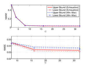
Figure 3: NMSE versus the training sequence size $G$ where $N_{t}=375$, $M=5$, $M_{p}=2$, $N_{d}=GM_{p}$, $\rho=10$, $d_{s}=100\text{m}$, AS$=16.7^{\circ}$, and $v=3km/h$.

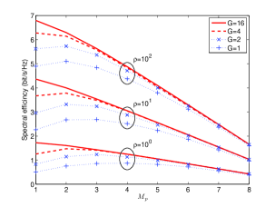
Figure 4: Spectral efficiency versus training period length $M_{p}$ where $N_{t}=375$, $M=10$, $N_{d}=GM_{p}$, $d_{s}=100\text{m}$, AS$=16.7^{\circ}$, and $v=3km/h$.

We adopt the one-ring channel model to generate each channel realization during simulation [37, 12]. The channel spatial correlation is characterized by angle spread (AS: $\Delta$), angle-of-arrival (AoA: $\theta$), and antenna geometry. Based on the one-ring channel model, we considered a $15\times 25$ uniform planar array at the base station. Then, the channel covariance matrix ${\bf R}_{\bf h}$ is given by ${\bf R}_{\bf h}={\bf R}_{H}\otimes{\bf R}_{V}$ where ${\bf R}_{H}\in\mathbb{C}^{N_{H}\times N_{H}}$ and ${\bf R}_{V}\in\mathbb{C}^{N_{V}\times N_{V}}$ denote the horizontal and vertical covariance matrices, respectively. Each of the spatial correlation matrices is defined by

$$[{\bf R}_{t}]_{p,q} =\frac{\gamma}{2\Delta}\int^{\theta+\Delta}_{\theta-\Delta}e^{-j\pi(p-q)\sin(\xi)}d\xi,$$ (35)

where $t\in\{H,V\}$ and $\gamma$ denotes propagation path loss between the transmitter and the receiver given by $\gamma=(1+(\frac{d_{s}}{d_{0}})^{\alpha_{0}})^{-1}$, where the path loss exponent is set to $\alpha_{0}=3.8$, $d_{s}$ is the distance from the transmitter in meters, and $d_{0}$ is the reference distance set to $d_{0}=30\text{m}$ [12]. We assume that the transmit antenna is located at an elevation of $h=60\text{m}$ and the local scattering ring around the user has radius $d_{r}=30\text{m}$. Then, the parameters for the channel covariance matrices ${\bf R}_{V}$ and ${\bf R}_{H}$ are given by $\Delta_{V}=\frac{1}{2}\left(\arctan(\frac{d_{s}+d_{r}}{h})-\arctan(\frac{d_{s}-d_{r}}{h})\right)$, $\theta_{V}=\frac{1}{2}\left(\arctan(\frac{d_{s}+d_{r}}{h})+\arctan(\frac{d_{s}-d_{r}}{h})\right)$, $\Delta_{H}=\arctan(\frac{d_{r}}{d_{s}})$, and $\theta_{H}\in(-\frac{\pi}{3},\frac{\pi}{3})$ for a sector in a cell.

V-A Practical Guidelines for Training Sequence

In this subsection, a practical guideline for training sequence parameters is developed with quantitative analysis.

First, we can improve channel estimation performance by choosing the row length of ${\bf C}$ large enough to incorporate more dominant eigen-directions of the channel in the $G\times M_{p}$ training sequence. Intuitively, the channel MSE of the $nG\times M_{p}$ training sequence ($n\in\mathbb{N}$) is at least equal to those of the $G\times M_{p}$ training sequence by $n$ times repetition of the shorter version of the training sequence. Fig. 3 shows the closed-form expressions of the upper and lower bounds in (14) and (16). It is seen that increasing $G$ is indeed beneficial in terms of the channel MSE, but the effect becomes marginal when $G$ is too large. That is, the proposed training sequence can operate in a finite $G$ regime and achieve reasonably good channel estimation performance, which implies that increasing the training period length $M_{p}$ also has similar effect on the channel MSE due to the increased training sequence size.

Second, though the increased $M_{p}$ enables large beamforming gain by leveraging channel estimation performance, an increment of $M_{p}$ can degrade achievable data rate because the remaining $M-M_{p}$ channel uses are only available for downlink data transmission. Therefore, we examine the trade-off of spectral efficiency in (33) corresponding to the value of $M_{p}$, which was obtained by using Algorithm 1 for simplicity. In Fig. 4, when the value of $G$ is small, the spectral efficiency benefits from the slightly increased $M_{p}$ since increasing $M_{p}$ enables the $G\times M_{p}$ training sequence to incorporate more dominant directions of the channel for channel estimation accuracy. However, increasing $M_{p}$ over some threshold limits the spectral efficiency due to the shorter length of data transmission period, as expected from the pre-log factor in (33). The tension between channel estimation accuracy and achievable data rate yields that the value of $M_{p}$ should be properly selected under given system parameters. Instead of this nontrivial choice, we can again increase the (vertical) sequence size $G$ for channel estimation accuracy without affecting the pre-log term. Fig. 4 shows that the increased $G$ makes the spectral efficiency quite insensitive w.r.t. $M_{p}$ for the practical range of the value of $G$.

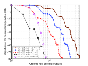
Figure 5: The magnitude of the normalized non-zero eigenvalues of ${\bf R}_{\bf h}$ where $\text{rank}({\bf R}_{\bf h})=r$.

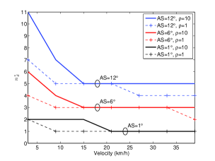
Figure 6: The optimized value of $n_{d}^{*}$ for training sequence and transmit precoding where $N_{t}=375$, $M=5$, $M_{p}=1$, $G=32$, $N_{d}=GM_{p}$, and $d_{s}=150\text{m}$.

Furthermore, we focus on the optimal number of dimensionality variable $n_{d}^{*}$ (or the number of active RF chains in the case of hybrid precoding) obtained from the proposed method. The reduced dimensionality $n_{d}^{*}$ used for training sequence and transmit beamforming design provides insight into the (effective) dominant channel rank considered for transmitting multiple data streams or the beamforming gain. Fig. 5 shows the magnitude of the eigenvalues of ${\bf R}_{\bf h}$, which is rank-deficient due to insufficient scatterers around a tower-mounted base station and a high angular resolution due to its large aperture. The rank of ${\bf R}_{\bf h}$ is determined by a few dominant eigenvalues and the number of less significant eigenvalues. Fig. 6 shows that, at high SNR, more training beam patterns are used to incorporate sufficient channel gains by subspace sampling in a sufficient broad space. On the other hand, a small number of training beamforming vectors are required to account for the most dominant eigen-directions of the channel, in the low-SNR regime. In addition, the user’s mobility also affects the value of $n_{d}^{*}$ because the estimated channel is more likely outdated in the fast-mobility case. Thus, one can mitigate the channel aging effect on the most dominant eigen-directions by properly reducing the dimension of the sampling subspace of the channel, i.e., properly reduce the number of unique training beam patterns $n_{d}$. This result indicates the influence of the various system parameters such as channel spatial correlation, angular spread, transmit power, and user terminals’ mobility on the effective channel rank based on the proposed method.

V-B Performance Evaluation of Training Techniques

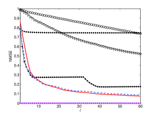
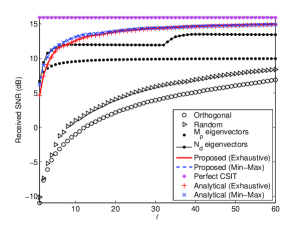
       (a) Channel estimation (same legend as in (b)) (b) Received SNR

Figure 7: NMSE and received SNR versus block time index $\ell$ where $N_{t}=375$, $M=5$, $M_{p}=2$, $G=32$, $N_{d}=64$, $\rho=10$, AS$=16.7^{\circ}$, and $v=3\text{km/h}$.

We compare the performance of the proposed methods to those of several downlink training techniques [38, 39, 40]. For all considered channel sounding methods, we use Kalman filtering for channel estimation. Fig. 7 shows the performance comparison with several training signal design methods [38, 39, 40] with $N_{t}=375~{}(N_{V}=15,N_{H}=25)$, $N_{d}=64$, $\theta_{H}=\frac{\pi}{6}$, and $d_{s}=100\text{m}$. Orthogonal and random training signals are chosen at the beginning of simulation and used in a round-robin manner. These methods are ineffective in terms of the amount of training duration for achieving reasonable channel estimation accuracy since such training signal patterns cannot effectively capture the dominant channel directions over all the $N_{t}$-dimensional space at each training period. The training signal composed of the fixed $M_{p}$ dominant eigenvectors of ${\bf R}_{\bf h}$ can only minimize the channel MSE in the limited subspace spanned by the fixed $M_{p}$ training vectors. Thus, the fixed training signal approach saturates quickly. We also consider the modified scheme that initially selects the $N_{d}$ dominant eigenvectors of ${\bf R}_{\bf h}$ and transmits $M_{p}$ training signals among the chosen $N_{d}$ training signal patterns across $G$ consecutive training periods where $N_{d}=GM_{p}$. The $N_{d}$ fixed training scheme shows the best performance up to the initial 7 blocks and becomes inefficient for the remaining duration. This result indicates that about 14 eigen-directions contain the most dominant channel gain which is not known a priori.

The proposed methods with the optimal number of training signal patterns $n_{d}^{*}=24$ substantially reduce the training duration necessary to achieve good channel estimation accuracy. This yields that the proper use of less dominant eigen-directions of the channel indeed leverages channel estimation performance. Within the first few blocks, the min-max approach in Algorithm 1 shows better performance than the exhaustive approach in Fig. 7(a). This is because the min-max training sequence is designed to sequentially minimize the dominant steady-state channel MSE, thus this approach shows a slightly steeper initial slope on the channel MSE. As a matter of fact, the exhaustive approach will eventually provide the best channel estimation performance, but only a marginal performance difference is observed in comparison with the min-max approach as shown in Table II. The proposed methods outperform other methods over almost all of transmission periods in terms of the channel MSE and the received SNR. Our simulation results also matches the analytic result of (48) very well in Fig. 7(b).

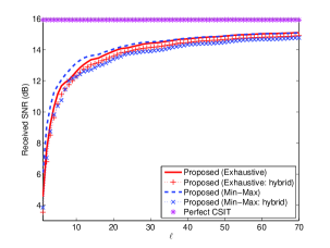
Figure 8: Received SNR versus block time index $\ell$ where $N_{t}=375$, $M=5$, $M_{p}=2$, $G=32$, $\rho=10$, AS$=16.7^{\circ}$, and $v=3\text{km/h}$.

Method	NMSE	Received SNR (dB)
Orthogonal	0.13	13.8
Random	0.13	13.8
$M_{p}$ eigenvectors	0.74	9.3
$N_{d}$ eigenvectors	0.05	14.9
Proposed (Exhaustive)	0.03	15.3
Proposed (Min-Max)	0.04	15.3
Proposed (Exhaustive: hybrid)	0.04	15.2
Proposed (Min-Max: hybrid)	0.05	15.2
Perfect CSIT	$0.00$	15.8

TABLE II: Steady-state performance: Comparison of several methods

Fig. 8 shows the performance of the proposed hybrid precoding design, where the DFT-based training sequence is used by exploiting the approximated channel spatial correlation ${\bf R}_{\bf h}$ in (22). It is seen that the proposed hybrid precoding method that uses imperfect channel correlation knowledge yields almost the same performance as the method with perfectly known ${\bf R}_{\bf h}$ during the transient phase in Fig. 8, and also shows a negligible performance difference in the steady-state phase as shown in Table II. An observation of practical importance is that the proposed hybrid precoding method based on a rough estimation of ${\bf R}_{\bf h}$ by using the DFT vectors seems to work well in FDD massive MIMO systems even with a limited number of RF chains for transmit beamforming. Due to space limitations, simulation results for a ray-based channel model are not provided, but our simulations using ray-based channel models have also yielded good channel estimation performance.

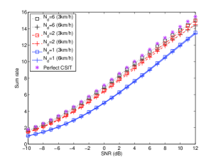
Figure 9: A lower bound on sum spectral efficiency versus SNR (dB) where $N_{t}=32$, $M=10$, $M_{p}=1$, AS$=4.6^{\circ}$, and $G=32$ in the multi-user case.

Finally, we evaluated the proposed method in the multiple-user situation with the ULA ($N_{t}=32$) at the base station to service $U$ users in a sector of a cell for the same setup as before in the one-ring model. We assume that users are uniformly distributed in a sector $\{\theta_{u}\in(-\pi/2,\pi/2):1\leq u\leq U\}$ with $d_{r}=8\text{m}$, $d_{s}=100\text{m}$, and $U=5$. Here, the SNR is defined as $\gamma\rho$ to account for the signal transmit power and the propagation path loss in (35). Fig. 9 shows that the performance of the lower bound on sum spectral efficiency in (34) under the several parameters of the dimensionality constraints $N_{d}$ and the terminal velocity. The performance of perfect CSIT case is shown as the performance reference. In Fig. 9, the proposed method achieves close performance of full CSIT with the reasonably increased dimensionality constraint.

VI Conclusion

We considered a reduced dimensionality training sequence and transmit precoder design aimed at enabling low-complexity and energy-efficient system implementation. We proposed a new method for training sequence design that leverages steady-state channel estimation performance in conjunction with Kalman filtering. The low-dimensionality constraint on training sequence and transmit precoding extends to a hybrid analog-digital precoding scheme that uses a limited number of active RF chains for transmit precoding by applying the Toeplitz distribution theorem with specific antenna configurations. We derived some necessary conditions for the optimal solution and provide a practical guideline for selecting the training sequence parameters along with performance analysis. The proposed method can provide a way to realize energy-efficient large-scale antenna systems.

-A Proof of Proposition 2

Given $g_{i}\geq g_{i}^{\prime}=g_{i}-c$ for some $0\leq c\leq g_{i}-1$, we have

$$\frac{a^{2g_{i}}}{1-a^{2g_{i}}}\leq\frac{a^{2g_{i}^{\prime}}}{1-a^{2g_{i}^{\prime}}} =\frac{a^{2g_{i}}}{1-a^{2g_{i}}}\gamma_{c},$$ (36)

where $\gamma_{c}:=\frac{1-a^{2g_{i}}}{a^{2c}-a^{2g_{i}}}\geq 1$. From (14) and (36), the channel MSE $\lambda_{i,g_{i}}^{\underline{\infty}}$ is increasing on $g_{i}$ as

$$\lambda_{i,g_{i}}^{(\underline{\infty})} =\frac{\lambda_{i}}{\bigl{(}\frac{1}{2}(1+\lambda_{i}\rho)\bigr{)}+\sqrt{\bigl{(}\frac{1}{2}(1+\lambda_{i}\rho)\bigr{)}^{2}+\frac{a^{2g_{i}}}{1-a^{2g_{i}}}\lambda_{i}\rho}}$$

$$\geq\frac{\lambda_{i}}{\bigl{(}\frac{1}{2}(1+\lambda_{i}\rho)\bigr{)}+\sqrt{\bigl{(}\frac{1}{2}(1+\lambda_{i}\rho)\bigr{)}^{2}+\frac{a^{2g_{i}}}{1-a^{2g_{i}}}\gamma_{c}\lambda_{i}\rho}}$$

$$=\lambda_{i,g_{i}^{\prime}}^{(\underline{\infty})}$$

In (16), $\lambda_{i,g_{i}}^{(\overline{\infty})}$ is a convex combination of $\lambda_{i,g_{i}}^{(\underline{\infty})}$ and $\lambda_{i}$ satisfying $\lambda_{i,g_{i}}^{(\underline{\infty})}<\lambda_{i}$ and thereby an increasing function as $g_{i}$ increases. Since the composite of increasing functions is increasing:

$$\lambda_{i,g_{i}^{\prime}}^{(\overline{\infty})} =a^{2(g_{i}^{\prime}-1)}\lambda_{i,g_{i}^{\prime}}^{(\underline{\infty})}+(1-a^{2(g_{i}^{\prime}-1)})\lambda_{i}$$

$$\leq a^{2(g_{i}-1)}\lambda_{i,g_{i}^{\prime}}^{(\underline{\infty})}+(1-a^{2(g_{i}-1)})\lambda_{i}$$

$$\leq a^{2(g_{i}-1)}\lambda_{i,g_{i}}^{(\underline{\infty})}+(1-a^{2(g_{i}-1)})\lambda_{i}=\lambda_{i,g_{i}}^{(\overline{\infty})},$$

we have the claim. $\hfill\blacksquare$

-B Proof of Proposition 3

For the proof of Proposition 3, it suffices to show that the matrix ${\bf C}$ of size $G\times M_{p}$ is constructed (i.e., $U_{j}=0$ for $1\leq j\leq M_{p}$) by allocating the $n_{d}$ eigenvector indices corresponding to the block time-wise interval $\{g_{1},\ldots,g_{n_{d}}\}$ since $\sum_{i=1}^{n_{d}}G/g_{i}=GM_{p}$ in (19).

The proof is by induction, where the notations follow those of Step (1) and Step (2). When $q=1$, let $U_{j}=G=p^{s}$ be the initial value for $1\leq j\leq M_{p}$ where given $\{g_{1},\ldots,g_{n_{d}}\}\in{\cal I}_{G}=\{1,p,\ldots,p^{s}\}$ as in (13). For any $1\leq q\leq G$, if $U_{j}\neq 0$, suppose that the unused $U_{j}$ entries at the $j$-th column can be described by the $n_{j}$ disjoint sets of equi-spacing $g_{i_{q,j}}=p^{k_{i_{q,j}}}\in{\cal I}_{G}$, i.e., $U_{j}=n_{j}\cdot p^{s-k_{i_{q,j}}}$ for some nonnegative integers $n_{j}$ and $k_{i_{q,j}}$. This means that the unused $U_{j}$ entries can be viewed as a collection of $n_{j}$ disjoint sets where the entries of each set are equi-spaced with $g_{i_{q,j}}=p^{k_{i_{q,j}}}$. Thus, after inserting the index of $i_{q,j}$ with a row-wise allocation at Step (1), $U_{j}$ is updated as $U_{j}=(n_{j}-1)\cdot p^{s-k_{i_{q,j}}}$.

In the subsequent iteration, if $U_{j}\neq 0$, there exist some row index $q^{\prime}>q$ such that we need to allocate the index of $i_{q^{\prime},j}$ using a row-wise mapping $g_{i_{q^{\prime},j}}$ starting from $[{\bf C}]_{q^{\prime},j}$ as shown in (20). Note that, by the assumption, it follows that $g_{i_{q^{\prime},j}}\geq g_{i_{q,j}}$. Since each set of equi-spacing $g_{i_{q},j}=p^{k_{i_{q,j}}}$ at the preceding step can be separated by the $g_{i_{q^{\prime},j}}/g_{i_{q},j}=p^{k_{i_{q^{\prime},j}}-k_{i_{q,j}}}$ disjoint subsets of equi-spacing $g_{i_{q^{\prime},j}}=p^{k_{i_{q^{\prime},j}}}$, the remaining $U_{j}$ entries can be viewed as the $(n_{j}-1)p^{k_{i_{q^{\prime},j}}-k_{i_{q,j}}}$ disjoint sets of equi-spacing $g_{i_{q^{\prime},j}}$, i.e., $U_{j}=((n_{j}-1)p^{k_{i_{q^{\prime},j}}-k_{i_{q,j}}})\cdot p^{s-k_{i_{q^{\prime},j}}}$. Therefore, it is possible to allocate the index of $i_{q^{\prime},j}$ into one of the disjoint sets of equi-spacing $g_{i_{q^{\prime},j}}$. We then update $n_{j}=(n_{j}-1)p^{k_{i_{q^{\prime},j}}-k_{i_{q,j}}}$ and $U_{j}=(n_{j}-1)\cdot p^{s-k_{i_{q^{\prime}},j}}$. Since this process repeats until $U_{j}\neq 0$ for all $j$, we have the claim. $\blacksquare$

Lemma 1

During the $\ell$-th training period, the channel estimate $\hat{{\bf h}}_{u,\ell|\ell}$ based on Kalman filtering is characterized by $E\{\hat{{\bf h}}_{u,\ell|\ell}\}=\mathbf{0}$ and $E\{\hat{{\bf h}}_{u,\ell|\ell}\hat{{\bf h}}_{u,\ell|\ell}^{H}\}={\bf R}_{{\bf h}_{u}}-{\bf P}_{u,\ell|\ell}$.

Proof: For notational simplicity, we omit the lower index $u$. From (5) and (6), the channel estimate $\hat{{\bf h}}_{\ell|\ell}$ for $\ell=0$ is given by

$$\hat{{\bf h}}_{0|0}={\bf P}_{0|-1}{\bf S}_{0}({\bf S}_{0}^{H}{\bf P}_{0|-1}{\bf S}_{0}+{\bf I}_{M_{p}})^{-1}{\bf y}_{0,pilot},$$ (37)

where recall that ${\bf y}_{\ell,pilot}=[y_{\ell M+1},\cdots,y_{\ell M+M_{p}}]^{T}$ denotes the $\ell$-th received training symbols and ${\bf S}_{u,\ell}=[{\bf s}_{u,\ell M+1}\cdots{\bf s}_{u,\ell M+M_{p}}]$ denotes the $\ell$-th training symbols, as shown in (4). Since $E\{{\bf y}_{0,pilot}{\bf y}_{0,pilot}^{H}\}={\bf S}_{0}^{H}{\bf P}_{0|-1}{\bf S}_{0}+{\bf I}_{M_{p}}$, we have

$$E\{\hat{{\bf h}}_{0|0}\hat{{\bf h}}_{0|0}^{H}\} ={\bf P}_{0|-1}{\bf S}_{0}({\bf S}_{0}^{H}{\bf P}_{0|-1}{\bf S}_{0}+{\bf I}_{M_{p}})^{-1}{\bf S}_{0}^{H}{\bf P}_{0|-1}$$

$$\stackrel{{\scriptstyle(a)}}{{=}}{\bf R}_{\bf h}-\bigl{(}{\bf P}_{0|-1}-{\bf P}_{0|-1}{\bf S}_{0}$$

$$~{}~{}~{}~{}({\bf S}_{0}^{H}{\bf P}_{0|-1}{\bf S}_{0}+{\bf I}_{M_{p}})^{-1}{\bf S}_{0}^{H}{\bf P}_{0|-1}\bigr{)}$$

$$={\bf R}_{\bf h}-{\bf P}_{0|0},$$

where $(a)$ holds by ${\bf P}_{0|-1}={\bf R}_{\bf h}$. Here, $E\{\hat{{\bf h}}_{0|0}\}=\mathbf{0}$ from $E\{{\bf y}_{0,pilot}\}={\bf S}_{0}^{H}E\{{\bf h}_{0}\}+E\{{\bf w}_{0}\}=\mathbf{0}$.

During the $\ell$-th training period, the channel estimate $\hat{{\bf h}}_{\ell|\ell}$ is given by from (6) and (8):

$$\hat{{\bf h}}_{\ell|\ell} =a\hat{{\bf h}}_{\ell-1|\ell-1}+{\bf P}_{\ell|\ell-1}{\bf S}_{\ell}({\bf S}_{\ell}^{H}{\bf P}_{\ell|\ell-1}{\bf S}_{\ell}+{\bf I}_{M_{p}})^{-1}$$

$$~{}~{}~{}({\bf y}_{\ell,pilot}-{\bf S}_{\ell}^{H}a\hat{{\bf h}}_{\ell-1|\ell-1}).$$ (38)

Denote by ${\bf e}_{\ell}\in\mathbb{C}^{M_{p}}$ the innovation process of Kalman filter given by

$${\bf e}_{\ell} ={\bf y}_{\ell,pilot}-{\bf S}_{\ell}^{H}(a\hat{{\bf h}}_{\ell-1|\ell-1})$$

$$=\left({\bf S}_{\ell}^{H}{\bf h}_{\ell}+{\bf w}_{\ell}\right)-{\bf S}_{\ell}^{H}(a\hat{{\bf h}}_{\ell-1|\ell-1})$$ (39)

$$\stackrel{{\scriptstyle(a)}}{{=}}\bigl{(}{\bf S}_{\ell}^{H}\bigl{(}a(\hat{{\bf h}}_{\ell-1|\ell-1}+\tilde{{\bf h}}_{\ell-1})+\sqrt{1-a^{2}}{\bf b}_{\ell}\bigr{)}+{\bf w}_{\ell}\bigr{)}$$

$$~{}~{}~{}-{\bf S}_{\ell}^{H}a\hat{{\bf h}}_{\ell-1|\ell-1}$$

$$={\bf S}_{\ell}^{H}\bigl{(}a\tilde{{\bf h}}_{\ell-1}+\sqrt{1-a^{2}}{\bf b}_{\ell}\bigr{)}+{\bf w}_{\ell},$$ (40)

where $(a)$ holds by (2) and $\tilde{{\bf h}}_{\ell}:={\bf h}_{\ell}-\hat{{\bf h}}_{\ell|\ell}$. Note that ${\bf e}_{\ell}$ is independent of $\hat{{\bf h}}_{\ell-1|\ell-1}$ due to the orthogonality property of the MMSE estimation and an independent process noise ${\bf b}_{\ell}$, then we have that ${\bf e}_{\ell}$ has zero mean and covariance matrix $E\{{\bf e}_{\ell}{\bf e}_{\ell}^{H}\}={\bf S}_{\ell}^{H}{\bf P}_{\ell|\ell-1}{\bf S}_{\ell}+{\bf I}_{M_{p}}$. Thus, we obtain $E\{\hat{{\bf h}}_{\ell|\ell}\}=aE\{\hat{{\bf h}}_{\ell-1|\ell-1}\}+{\bf K}_{\ell}E\{{\bf e}_{\ell}\}=\mathbf{0}$. From (38), $E\{\hat{{\bf h}}_{\ell|\ell}\hat{{\bf h}}_{\ell|\ell}^{H}\}$ is given by

$$E\{\hat{{\bf h}}_{\ell|\ell}\hat{{\bf h}}_{\ell|\ell}^{H}\}$$

$$=a^{2}E\{\hat{{\bf h}}_{\ell-1|\ell-1}\hat{{\bf h}}_{\ell-1|\ell-1}^{H}\}+{\bf K}_{\ell}E\{{\bf e}_{\ell}{\bf e}_{\ell}^{H}\}{\bf K}_{\ell}^{H}$$ (41)

$$=a^{2}({\bf R}_{\bf h}-{\bf P}_{\ell-1|\ell-1})$$

$$~{}~{}~{}+\bigl{(}{\bf P}_{\ell|\ell-1}{\bf S}_{\ell}({\bf S}_{\ell}^{H}{\bf P}_{\ell|\ell-1}{\bf S}_{\ell}+{\bf I}_{M_{p}})^{-1}{\bf S}_{\ell}^{H}{\bf P}_{\ell|\ell-1}\bigr{)}$$ (42)

$$=a^{2}{\bf R}_{\bf h}-\bigl{(}{\bf P}_{\ell|\ell-1}-(1-a^{2}){\bf R}_{\bf h}\bigr{)}$$

$$~{}~{}~{}+\bigl{(}{\bf P}_{\ell|\ell-1}{\bf S}_{\ell}({\bf S}_{\ell}^{H}{\bf P}_{\ell|\ell-1}{\bf S}_{\ell}+{\bf I}_{M_{p}})^{-1}{\bf S}_{\ell}^{H}{\bf P}_{\ell|\ell-1}\bigr{)}$$ (43)

$$={\bf R}_{\bf h}-\bigl{(}{\bf P}_{\ell|\ell-1}-{\bf P}_{\ell|\ell-1}{\bf S}_{\ell}({\bf S}_{\ell}^{H}{\bf P}_{\ell|\ell-1}{\bf S}_{\ell}+{\bf I}_{M_{p}})^{-1}$$

$$~{}~{}~{}~{}{\bf S}_{\ell}^{H}{\bf P}_{\ell|\ell-1}\bigr{)}$$

$$={\bf R}_{\bf h}-{\bf P}_{\ell|\ell},$$ (44)

where the equality (43) follows (8). Since this Kalman recursion repeats, we have the claim. $\hfill\blacksquare$

-C Proof of Proposition 4

To derive the deterministic quantity for $SINR_{u,\ell}$ in the limit of $N_{t}\rightarrow\infty$, we use the analysis technique [6]. Applying Lemma 1, we have

$$\frac{1}{N_{t}^{2}}|\hat{{\bf h}}_{u,\ell|\ell}^{H}\hat{{\bf h}}_{u,\ell|\ell}|^{2}-\frac{1}{N_{t}^{2}}|\text{tr}({\bf R}_{{\bf h}_{u}}-{\bf P}_{u,\ell|\ell})|^{2}~{}\begin{subarray}{c}a.s.\\ \overrightarrow{N_{t}\rightarrow\infty}\end{subarray}~{}0,$$ (45)

where $\begin{subarray}{c}a.s.\\ \longrightarrow\end{subarray}$ denotes the almost sure convergence. If $u\neq u^{\prime}$, then ${\bf h}_{u,\ell}$ and $\hat{{\bf h}}_{u^{\prime},\ell|\ell}$ are mutually independent, thus we have using Lemma 1 as

$$\frac{1}{N_{t}^{2}}|{\bf h}_{u,\ell}^{H}\hat{{\bf h}}_{u^{\prime},\ell|\ell}|^{2}-\frac{1}{N_{t}^{2}}\text{tr}\left({\bf R}_{{\bf h}_{u}}({\bf R}_{{\bf h}_{u^{\prime}}}-{\bf P}_{u^{\prime},\ell|\ell})\right)~{}\begin{subarray}{c}a.s.\\ \overrightarrow{N_{t}\rightarrow\infty}\end{subarray}~{}0,$$ (46)

Since $\tilde{{\bf h}}_{u,\ell}$ is independent of $\hat{{\bf h}}_{u,\ell|\ell}$ by the orthogonality property of the MMSE estimate, we obtain by using Lemma 1 and $\tilde{{\bf h}}_{u,\ell|\ell}\sim\mathcal{CN}(\mathbf{0},{\bf P}_{u,\ell|\ell})$ as

$$\frac{1}{N_{t}^{2}}|\tilde{{\bf h}}_{u,\ell}^{H}\hat{{\bf h}}_{u,\ell|\ell}|^{2}-\frac{1}{N_{t}^{2}}\text{tr}\left({\bf P}_{u,\ell|\ell}({\bf R}_{{\bf h}_{u}}-{\bf P}_{u,\ell|\ell})\right)~{}\begin{subarray}{c}a.s.\\ \overrightarrow{N_{t}\rightarrow\infty}\end{subarray}~{}0.$$ (47)

Substituting (45), (46), and (47) into (30) with $\alpha_{u}^{2}=(\text{tr}({\bf R}_{{\bf h}_{u}}-{\bf P}_{u,\ell|\ell}))^{-1}$ for $1\leq u\leq U$, we have the deterministic equivalent SINR, given by

$$\overline{SINR}_{u,\ell} =|\text{tr}({\bf R}_{{\bf h}_{u}}-{\bf P}_{u,\ell|\ell})|^{2}$$

$$\left(\frac{1}{\alpha_{u}^{2}\rho}+\text{tr}\left({\bf P}_{u,\ell|\ell}({\bf R}_{{\bf h}_{u}}-{\bf P}_{u,\ell|\ell})\right)\right.$$

$$\left.+\sum_{u^{\prime}=1:u^{\prime}\neq u}^{U}\frac{\alpha_{u^{\prime}}^{2}}{\alpha_{u}^{2}}\text{tr}\left({\bf R}_{{\bf h}_{u}}({\bf R}_{{\bf h}_{u^{\prime}}}-{\bf P}_{u^{\prime},\ell|\ell})\right)\right)^{-1}.$$ (48)

Note that the estimation error covariance matrix ${\bf P}_{u,\ell|\ell}$ has the same set of eigenvectors of ${\bf R}_{{\bf h}_{u}}$ over all $\ell$ when we use its eigenvectors as the training signals [9]. That is, given the ED of ${\bf R}_{{\bf h}_{u}}={\bf U}_{u}\mbox{$\bf\Lambda$}_{u}{\bf U}_{u}^{H}$, ${\bf P}_{u,\ell|\ell}$ is eigen-decomposed by ${\bf P}_{u,\ell|\ell}={\bf U}_{u}\bar{\mbox{$\bf\Lambda$}}_{u}^{(\ell)}{\bf U}_{u}^{H}$. From $\text{tr}({\bf A}{\bf B}{\bf C})=\text{tr}({\bf B}{\bf C}{\bf A})$, the terms in (48) are then given by

$$\text{tr}({\bf R}_{{\bf h}_{u}}-{\bf P}_{u,\ell|\ell}) =\text{tr}(\mbox{$\bf\Lambda$}_{u}-\bar{\mbox{$\bf\Lambda$}}_{u}^{(\ell)})$$ (49)

$$\text{tr}\left({\bf R}_{{\bf h}_{u}}({\bf R}_{{\bf h}_{u^{\prime}}}-{\bf P}_{u^{\prime},\ell|\ell})\right) =\text{tr}\bigl{(}\mbox{$\bf\Lambda$}_{u}{\bf U}_{u}^{H}{\bf U}_{u^{\prime}}$$

$$(\mbox{$\bf\Lambda$}_{u^{\prime}}-\bar{\mbox{$\bf\Lambda$}}_{u^{\prime}}^{(\ell)}){\bf U}_{u^{\prime}}^{H}{\bf U}_{u}\bigr{)}$$ (50)

$$\text{tr}\left({\bf P}_{u,\ell|\ell}({\bf R}_{{\bf h}_{u^{\prime}}}-{\bf P}_{u^{\prime},\ell|\ell})\right) =\text{tr}\bigl{(}\bar{\mbox{$\bf\Lambda$}}_{u}^{(\ell)}(\mbox{$\bf\Lambda$}_{u}-\bar{\mbox{$\bf\Lambda$}}_{u}^{(\ell)})\bigr{)}$$ (51)

By substituting (49), (50), and (51) into (48), the SINR expression is rewritten as (31). $\hfill\blacksquare$

-D Derivation of the lower bound in (34)

By substituting ${\bf g}_{u}\in\mathbb{N}^{n_{d}}$ into (14) and (16), we can derive ${\hbox{\boldmath$\lambda$\unboldmath}}_{{\bf g}_{u}}^{(\underline{\infty})}$ and ${\hbox{\boldmath$\lambda$\unboldmath}}_{{\bf g}_{u}}^{(\overline{\infty})}$. From an inequality of (17), it follows that

$$\bigl{\|}\hbox{\boldmath$\lambda$\unboldmath}_{u}-{\hbox{\boldmath$\lambda$\unboldmath}}_{{\bf g}_{u}}^{(\overline{\infty})}\bigr{\|}_{1} \leq\lim_{\ell\rightarrow\infty}\bigl{\|}\hbox{\boldmath$\lambda$\unboldmath}_{u}-\bar{\hbox{\boldmath$\lambda$\unboldmath}}_{{\bf g}_{u}}^{(\ell)}\bigr{\|}_{1}$$

$$\lim_{\ell\rightarrow\infty}\bigl{\|}\bar{\hbox{\boldmath$\lambda$\unboldmath}}_{{\bf g}_{u}}^{(\ell)}\odot(\hbox{\boldmath$\lambda$\unboldmath}_{u}-\bar{\hbox{\boldmath$\lambda$\unboldmath}}_{{\bf g}_{u}}^{(\ell)})\bigr{\|}_{1} \leq\bigl{\|}{\hbox{\boldmath$\lambda$\unboldmath}}_{{\bf g}_{u}}^{(\overline{\infty})}\odot(\hbox{\boldmath$\lambda$\unboldmath}_{u}-{\hbox{\boldmath$\lambda$\unboldmath}}_{{\bf g}_{u}}^{(\underline{\infty})})\bigr{\|}_{1}$$

$$\lim_{\ell\rightarrow\infty}\text{tr}\bigl{(}\mbox{$\bf\Lambda$}_{u}{\bf U}_{u}^{H}{\bf U}_{u^{\prime}}(\mbox{$\bf\Lambda$}_{u^{\prime}}- \bar{\mbox{$\bf\Lambda$}}_{{\bf g}_{u^{\prime}}}^{(\ell)}){\bf U}_{u^{\prime}}^{H}{\bf U}_{u}\bigr{)}$$

$$\leq\text{tr}\bigl{(}\mbox{$\bf\Lambda$}_{u}{\bf U}_{u}^{H} {\bf U}_{u^{\prime}}(\mbox{$\bf\Lambda$}_{u^{\prime}}-{\mbox{$\bf\Lambda$}}_{{\bf g}_{u^{\prime}}}^{(\underline{\infty})}){\bf U}_{u^{\prime}}^{H}{\bf U}_{u}\bigr{)},$$ (52)

where ${\bf P}_{u,\ell|\ell}={\bf U}_{u}\bar{\mbox{$\bf\Lambda$}}_{u}^{(\ell)}{\bf U}_{u}^{H}$ with $\bar{\mbox{$\bf\Lambda$}}_{u}^{(\ell)}=\text{diag}(\bar{\hbox{\boldmath$\lambda$\unboldmath}}_{{\bf g}_{u}}^{(\ell)})$, ${\mbox{$\bf\Lambda$}}_{{\bf g}_{u^{\prime}}}^{(\underline{\infty})}=\text{diag}({\hbox{\boldmath$\lambda$\unboldmath}}_{{\bf g}_{u^{\prime}}}^{(\underline{\infty})})$, and the initial conditions (5). By applying the inequalities (-D) to (31), we obtain the closed-form lower bound on the steady-state SINR, as shown in (34). $\hfill\blacksquare$

References

- [1] S. Noh, M. D. Zoltowski, and D. J. Love, “Downlink training codebook design and hybrid preceding in FDD massive MIMO systems,” in Proc. IEEE Global Commun. Conf., Dec. 2014.
- [2] M. D. Renzo, H. Haas, A. Ghrayeb, S. Sugiura, and L. Hanzo, “Spatial modulation for generalized MIMO: Challenges, opportunities and implementation,” in Proc. IEEE, Jan. 2014, vol. 102, pp. 56 – 103.
- [3] T. L. Marzetta, “Noncooperative cellular wireless with unlimited numbers of base station antennas,” IEEE Trans. Wireless Commun., vol. 9, no. 11, pp. 3590 – 3600, Nov. 2010.
- [4] F. Rusek, D. Persson, B. K. Lau, E. G. Larsson, O. Edfors, F. Tufvesson, and T. L. Marzetta, “Scaling up MIMO: Opportunities and challenges with very large arrays,” IEEE Signal Process. Mag., vol. 30, no. 1, pp. 40 – 60, Jan. 2013.
- [5] J. Jose, A. Ashikhmin, T. L. Marzetta, and S. Vishwanath, “Pilot contamination and precoding in multi-cell TDD systems,” IEEE Trans. Wireless Commun., vol. 10, no. 8, pp. 2640 – 2651, Aug 2011.
- [6] J. Hoydis, S. ten Brink, and M. Debbah, “Massive MIMO in the UL/DL of cellular networks: How many antennas do we need?,” IEEE J. Sel. Areas Commun., vol. 31, no. 2, pp. 160 – 171, Feb. 2013.
- [7] C. Shepard, H. Yu, N. Anand, L. E. Li, T. L. Marzetta, R. Yang, and L. Zhong, “Argos: Practical many-antenna base stations,” in Proc. MobiCom, Istanbul, Turkey, Aug. 2012.
- [8] S. Noh, M. D. Zoltowski, Y. Sung, and D. J. Love, “Optimal pilot beam pattern design for massive MIMO systems,” in Proc. Asilomar Conf. on Signal, Syst. and Comput., Pacific Grove, CA, Nov. 2013.
- [9] S. Noh, M. D. Zoltowski, Y. Sung, and D. J. Love, “Pilot beam pattern design for channel estimation in massive MIMO systems,” IEEE J. Sel. Topics Signal Process., vol. 8, no. 5, pp. 787 – 801, Oct. 2014.
- [10] J. Choi, Z. Chance, D. J. Love, and U. Madhow, “Noncoherent trellis coded quantization: A practical limited feedback technique for massive MIMO systems,” IEEE Trans. Commun., vol. 61, no. 12, pp. 5016 – 5029, Dec. 2013.
- [11] J. Choi, D. J. Love, and P. Bidigare, “Downlink training techniques for FDD massive MIMO systems: Open-loop and closed-loop training with memory,” IEEE J. Sel. Topics Signal Process., vol. 8, no. 5, pp. 802 – 814, Oct. 2014.
- [12] A. Adhikary, J. Nam, J.-Y. Ahn, and G. Caire, “Joint spatial division and multiplexing: The large-scale array regime,” IEEE Trans. Inf. Theory, vol. 59, no. 10, pp. 6441 – 6463, Oct. 2013.
- [13] A. Adhikary and G. Caire, “Joint spatial division and multiplexing: Opportunistic beamforming and user grouping,” IEEE J. Sel. Topics Signal Process., vol. 8, no. 5, pp. 876 – 890, Oct. 2014.
- [14] G. Lee and Y. Sung, “A new approach to user scheduling in massive multi-user MIMO broadcast channels,” IEEE Trans. Inf. Theory, submitted for publication. [Online]. Available: http://arxiv.org/abs/1403.6931, 2014.
- [15] J. So, D. Kim, Y. Lee, and Y. Sung, “Pilot signal design for massive MIMO systems: A received signal-to-noise-ratio-based approach,” IEEE Signal Process. Lett., vol. 52, no. 5, pp. 549 – 553, May 2015.
- [16] J. Hoydis, C. Hoek, T. Wild, and S. ten Brink, “Channel measurements for large antenna arrays,” in Proc. IEEE Int. Symp. Wireless Commun. Syst., Paris, France, Aug. 2012.
- [17] X. Gao, O. Edfors, F. Rusek, and F. Tufvesson, “Linear pre-coding performance in measured very-large MIMO channels,” in Proc. IEEE Veh. Technol. Conf., San Francisco, CA, Sep. 2011.
- [18] S. Wagner, R. Couillet, M. Debbah, and D.T.M. Slock, “Large system analysis of linear precoding in correlated MISO broadcast channels under limited feedback,” IEEE Trans. Inf. Theory, vol. 58, no. 7, pp. 4509 – 4537, Mar. 2012.
- [19] H. Q. Ngo, E. G. Larsson, and T. L. Marzetta, “The multi cell multiuser MIMO uplink with very large antenna arrays and a finite-dimensional channel,” IEEE Trans. Commun., vol. 61, no. 6, pp. 2350 – 2361, Jun. 2013.
- [20] R. Kudo, S. Armour, J. McGeehan, and M. Mizoguchi, “A channel state information feedback method for massive MIMO-OFDM,” IEEE J. Commun. Netw., vol. 15, no. 4, pp. 352 – 361, Aug. 2013.
- [21] P.-H. Kuo, H. T. Kung, and P.-A. Ting, “Compressive sensing based channel feedback protocols for spatially-correlated massive antenna arrays,” in Proc. IEEE Wireless Commun. Netw. Conf., Paris, France, Apr. 2012.
- [22] X. Rao and V. Lau, “Distributed compressive CSIT estimation and feedback for FDD multi-user massive MIMO systems,” IEEE Trans. Signal Process., vol. 62, no. 12, pp. 3261 – 3271, Jun. 2014.
- [23] L. Tong, B. M. Sadler, and M. Dong, “Pilot-assisted wireless transmissions: General model, design criteria, and signal processing,” IEEE Signal Process. Mag., vol. 21, no. 6, pp. 12 – 25, Nov. 2004.
- [24] W. C. Jakes, Microwave Mobile Communication, Wiley, New York, NY, 1974.
- [25] G. Matz, “On non-WSSUS wireless fading channels,” IEEE Trans. Wireless Commun., vol. 4, no. 5, pp. 2465 – 2478, Sep. 2005.
- [26] A. Ispas, M. Drpinghaus, G. Ascheid, and T. Zemen, “Characterization of non-stationary channels using mismatched Wiener filtering,” IEEE Trans. Signal Process., vol. 61, no. 2, pp. 274 – 288, Jan. 2013.
- [27] T. Kailath, A. H. Sayed, and B. Hassibi, Linear Estimation, Prentice-Hall, Upper Saddle River, New Jersey, 2000.
- [28] M. Dong, L. Tong, and B. M. Sadler, “Optimal insertion of pilot symbols for transmissions over time-varying flat fading channels,” IEEE Trans. Signal Process., vol. 52, no. 5, pp. 1403 – 1418, May 2004.
- [29] A. M. Sayeed, “Deconstructing multi antenna fading channels,” IEEE Trans. Signal Process., vol. 50, no. 10, pp. 2563 – 2579, Oct. 2002.
- [30] S. Wu, C.-X. Wang, el H. M. Aggoune, M. M. Alwakeel, and Y. He, “A non-stationary 3-D sideband twin-cluster model for 5G massive MIMO channels,” IEEE J. Sel. Areas Commun., vol. 32, no. 6, pp. 1207 – 1218, Jun. 2014.
- [31] U. Grenander and G. Szegö, Toeplitz Forms and Their Applications, University of California Press, Berkeley, CA, 1958.
- [32] Y. Sung, H. V. Poor, and H. Yu, “How much information can one get from a wireless ad hoc sensor network over a correlated random field?,” IEEE Trans. Inf. Theory, vol. 55, no. 6, pp. 2827 – 2847, Jun. 2009.
- [33] A. F. Molisch, “A generic model for MIMO wireless propagation channels in macro- and microcells,” IEEE Trans. Signal Process., vol. 52, no. 1, pp. 61 – 71, Jan. 2004.
- [34] A. Forenza, D. J. Love, and R. W. Heath Jr., “Simplified spatial correlation models for clustered MIMO channels with different array configurations,” IEEE Trans. Veh. Technol., vol. 56, no. 4, pp. 1924 – 1934, Jul. 2007.
- [35] O. E. Ayach, S. Rajagopal, S. Adu-Surra, Z. Pi, and R. W. Heath Jr., “Spatially sparse precoding in millimeter wave MIMO systems,” IEEE Trans. Wireless Commun., vol. 13, no. 3, pp. 1499 – 1513, Mar. 2014.
- [36] B. Hassibi and B. M. Hochwald, “How much training is needed in multiple-antenna wireless links?,” IEEE Trans. Inf. Theory, vol. 49, no. 4, pp. 951 – 963, Apr. 2003.
- [37] D. Shiu and G. J. Foschini and M. J. Gans and J. M. Kahn, “Fading correlation and its effect on the capacity of multi element antenna systems,” IEEE Trans. Commun., vol. 48, no. 3, pp. 502 – 513, Mar. 2000.
- [38] W. Santipach and M. L. Honig, “Optimization of training and feedback overhead for beamforming over block fading channels,” IEEE Trans. Inf. Theory, vol. 56, no. 12, pp. 6103 – 6115, Dec. 2010.
- [39] F. Kaltenberger, M. Kountouris, D. Gesbert, and R. Knopp, “On the trade-off between feedback and capacity in measured MU-MIMO channels,” IEEE Trans. Wireless Commun., vol. 8, no. 9, pp. 4866 – 4875, Sep. 2009.
- [40] J. H. Kotecha and A. M. Sayeed, “Transmit signal design for optimal estimation of correlated MIMO channels,” IEEE Trans. Signal Process., vol. 52, no. 2, pp. 546 – 557, Feb. 2004.