Nanometer-scale Tomographic Reconstruction of 3D Electrostatic Potentials in GaAs/AlGaAs Core-Shell Nanowires

Abstract

We report on the development of Electron Holographic Tomography towards a versatile potential measurement technique, overcoming several limitations, such as a limited tilt range, previously hampering a reproducible and accurate electrostatic potential reconstruction in three dimensions. Most notably, tomographic reconstruction is performed on optimally sampled polar grids taking into account symmetry and other spatial constraints of the nanostructure. Furthermore, holographic tilt series acquisition and alignment have been automated and adapted to three dimensions. We demonstrate $6$ nm spatial and $0.2$ V signal resolution by reconstructing various, previously hidden, potential details of a GaAs/AlGaAs core-shell nanowire. The improved tomographic reconstruction opens pathways towards the detection of minute potentials in nanostructures and an increase in speed and accuracy in related techniques such as X-ray tomography.

Tomographic techniques use lower dimensional projections of $n$-dimensional data to reconstruct the original quantity. This principle dates back to the work of the Austrian mathematician J. Radon Radon (1917) and to date applications in fields as diverse as medicine, geophysics, material science and quantum information are reported. Our main goal is the tomographic reconstruction of 3D electrostatic potentials in nanostructures. They are tightly connected to the chemical composition and electronic structure and therefore mirror the corresponding functionality and possible failures. Off-axis electron holography (EH) provides unique access to these fields Dunin-Borkowski et al. (2004); Lichte and Lehmann (2008); Midgley and Dunin-Borkowski (2009) because the reconstructed phase is in the phase grating approximation proportional to the potential projected along lines $l$

$$\varphi\left(x,p\right)=\left(C_{E}\int_{l\left(x,p,\theta\right)}V\left(\mathbf{r}\right)\mathrm{d}s\right)\,\mathrm{mod}\left(2\pi\right)$$ (1)

which holds for a wide range of imaging conditions Matteucci et al. (2002). Here, $C_{E}$ denotes the electron-matter interaction constant depending only on the acceleration voltage of the electrons ($C_{E}=6.5$ mrad/(Vnm) @ 300 kV), $\left(x,p,\theta\right)^{T}$ the coordinates of the detector, and $\mathbf{r}=\left(x,y,z\right)^{T}$ the coordinates in real space as explained in Fig. 2. In particular the $x$-axis is set parallel to the tilt axis in order to reduce the 3D reconstruction to a slice by slice 2D tomographic reconstruction problem in planes perpendicular to the tilt axis.

Following the mathematical foundations of tomography (e.g. Natterer (2001)), the collection of projected potentials (1) under different angles $\theta$ represents the Radon transform $\hat{V}=\mathit{\mathcal{R}}\left\{V\right\}$ of $V$. The inversion of this transformation (inverse Radon transformation) then yields the potential $V=\mathit{\mathcal{R}}^{-1}\left\{\hat{V}\right\}$ forming the basis of EH tomography (EHT). The proof-of-concept for EHT dates back to the work of Lai et al. Lai et al. (1994), however, quantitative reconstructions Twitchett-Harrison et al. (2007); Fujita and Chen (2009); Wolf et al. (2010) were delayed for a long time mainly for two reasons: first, the instrumental demands, such as specific tomography specimen holders allowing ultrahigh tilt angles, nanometer precise computer-controlled goniometers as well as powerful computers had to be developed. Second, the EHT procedure is very comprehensive and time consuming.

The most notable experimental limitation of virtual all electron-microscopic tomographic techniques is the limited tilt range of usually ±70° instead of ±90°. This leads to a loss of information, visible as “missing wedge” in the Fourier transform of the tomogram (see e.g. Midgley and Weyland (2003)). In real space, this corresponds to a reduced resolution in the tomogram in the direction of the missing wedge. Moreover, dynamical scattering effects, tilt axis misalignment, phase unwrapping failures and shot noise introduce errors in the projected data that can amplify upon reconstruction because of the (mildly) ill-conditioned nature of the Radon transform Natterer (2001). Similar to other tomographic techniques, large and ongoing efforts are therefore put into developing regularization schemes ($\cong$suppressing the error amplification) typically involving auxiliary conditions such as (euclidean) norm minimization ($\cong$Tikhonov regularization Tikhonov and Arsenin (1977)), total variation minimization ($\cong$generalized Tikhonov regularization Goris et al. (2012)) or signal range restriction (discrete tomography Batenburg et al. (2009)). Since such conditions typically introduce an additional regularization error, the art of regularization consists of minimizing the total error of both original and regularization error. That task is further complicated by the fact that these errors are generally unknown Hansen (1998). It is therefore always advantageous to use preferably error-free conditions based on real physical properties of the potential such as physical spatial constraints (e.g. Twitchett-Harrison et al. (2007)). That can be due to outer or internal boundaries of nanoparticles or symmetries imposed by the crystal structure.

How spatial constraints can be used to improve the tomographic reconstruction will be discussed in the following section. We will furthermore emphasize the importance of sampling, that is, the relation between detector resolution, number of projection angles and reconstructed object features, for the design of optimal reconstruction algorithms. The obtained improvement will be valuable for all types of tomography in spite of our particular application to EHT. Our second focus are improving methods for phase unwrapping, dynamic scattering correction and tilt series alignment, mainly dedicated to EHT. The combination of which will significantly improve EHT as 3D potential reconstruction method.

Using the optimized reconstruction procedure we successfully retrieved the 3D potential of a $\left\langle 111\right\rangle$-oriented GaAs-Al_0.33Ga_0.67As core-shell nanowire (NW) grown by metal-organic vapor phase epitaxy (MOVPE) through a Au nanoparticles (NP) as metal catalyst (see Ref. Prete et al. (2008); Wolf et al. (2011)). The structure provides a wide range of electrostatic potentials with sharp interfacesas well as long rang gradients. The AlGaAs shell contains also self-assembled Al segregations and local alloy fluctuations due to the different Ga and Al adatom mobilities on the nanowire surface Rudolph et al. (2013); Heiss et al. (2013). Note that these features are crucial for envisaged applications of semiconductor NW in future nano-scaled electronic, optoelectronic, and photovoltaic devices Bryllert et al. (2006); Gallo et al. (2011); Krogstrup et al. (2013). Moreover, we previously investigated this system with less developed EHT techniques Wolf et al. (2011), rendering it the ideal test case for verifying the achieved progress.

I Algebraic Holographic Tomography

The general workflow of EHT consisting of hologram tilt series acquisition, phase reconstruction from hologram tilt series; phase tilt series alignment and tomographic reconstruction is depicted in Fig. 2 using the example of the GaAs-AlGaAs NW. All steps have been widely automated, not only to decrease the amount of time from initially $\mathcal{O}\left(10\,\mathrm{h}\right)$ to presently $\mathcal{O}\left(1\,\mathrm{h}\right)$ (see Wolf et al. (2010) for details), but also to increase the reproducibility and quality of the obtained data. Thus, the automated workflow is an important prerequisite towards widespread application. The holographic tilt series of an individual NW with an entire diameter of 300 nm (80 nm core, 110 nm shell) was recorded in a range from $-69\text{\textdegree}$ to $+72\text{\textdegree\ in $3\text{\textdegree}$}$ steps at the FEI Titan 80-300 Berlin Holography Special TEM using the THOMAS software package Wolf et al. (2010). The TEM was operated at 300 kV acceleration voltage in aberration corrected Lorentz mode that provides a resolution of about $2\,\mathrm{nm}$. The holograms were acquired with a double biprism setup with a field of view of 1 $\mathrm{\mu}$m and a fringe spacing of 3 nm. The object exit wave tilt series has been reconstructed from the object holograms and corresponding empty holograms applying a Butterworth filter of $0.13\,\mathrm{nm^{-1}}$ FWHM to separate the side band (see e.g. in Lehmann and Lichte (2002) for further details of the holographic method). This was performed automatically for the entire tilt series. Fig. 1 shows a typical example of an holographically reconstructed projected potential of the NW. To highlight the effects in the vacuum region due to beam charging and remaining phase wedges due to the sideband alignment we also show the outer region in Fig. 1. Here, one observes a small charging field accumulating around 50 Vnm at the edge of the NW and dropping quickly to -50 Vnm towards the rim of the reconstruction volume. Considering that the whole NW has a diameter of 300 nm this corresponds to a surface potential due to charging of around 0.3 V. To test its influence on the tomographic reconstruction we performed the latter with and without constraining the complete vacuum to 0 V as stated in the results section below.

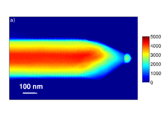
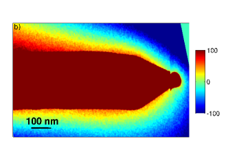
Figure 1: Examplary projected potential (in Vnm) reconstructed from a hologram of the tilt series (at 30° tilt angle) depicted at two different colour scales to illustrate the magnitude of the charging. On top the complete potential reachig several kVnm in the NW is depicted. The charging field below is approximately 2 order of magnitude lower and is also slightly superimposed by an additional phase wedge from the imperfect alignment of the sideband. The zero potential region on the top right stems from the alignment of the tilt axis along $x$.

Following holographic wave reconstruction and reorientation of the tilt axis along the $x$-axis, three important processing steps determine the accuracy of the subsequent tomographic reconstruction: (1) The phase needs to be unwrapped to obtain the projected potential from the reconstructed waves. The unwrapping is problematic if the sampled phase difference between two pixels exceeds $\pi$ Ghiglia and Pritt (1998), a situation often present in noisy data with sharp thickness jumps at specimen edges. We tackled this problem by extending the original 2D unwrapping performed at each holographic reconstruction to 3D with the tilt angle as third dimension (i.e. the whole tilt series). That is possible because of the continuous dependency of the phase on the tilt angle and yielded accurate projected potentials even at the Au catalyst. The next step (2) consists of suppressing dynamical scattering artifacts producing oscillations of the phase close to zone axis conditions (Fig. 2a)). The latter could be largely removed by normalizing the average of the projected potentials at all angles to the same value, in agreement with a dynamical correction factor approach Lubk et al. (2010). (3) Finally, this data is aligned around a common tilt axis with the center of mass method. This alignment was performed slice by slice for sampling reasons discussed below. The tilt series ready for tomographic reconstruction is depicted in Fig. 2b. Besides the substantial improvement of the data one observes a 6-fold symmetry in the core-shell region reducing to a 3-fold symmetry in the tapered section below the Au NP (corroborated by azimuthal cross-correlation in Fig. 2b).

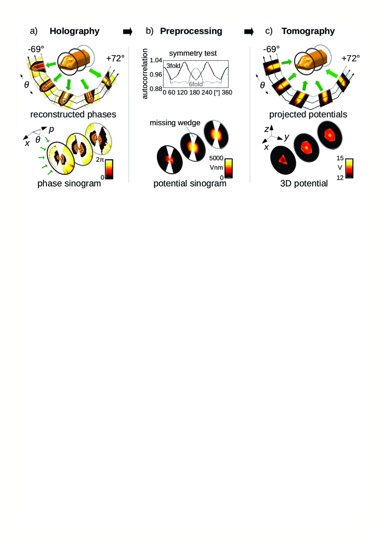
Figure 2: Holographic tomographic principle: a) Holographic tilt series (top) and selected sinograms (bottom). b) Rotational symmetry test (top) on preprocessed projected potential data (bottom). The 6-fold (hexagonal) symmetry of the NW is partly suppressed by the 2-fold symmetry of the missing wedge. c) Tomographic reconstruction (top) and reconstructed potential (bottom). Throughout the figure the 5 green arrows denote a set of angles ($-66\text{\textdegree},\,-33\text{\textdegree},\,0\text{\textdegree},\,33\text{\textdegree},\,66\text{\textdegree}$) and 3 deliberately chosen slices at $x=100,\,400,\,700$ nm are highlighted by black, dark gray and light gray lines and frames.

Now the actual tomographic reconstruction starts. The variety of reconstruction techniques can be separated into filtered, Fourier and algebraic algorithms, which coincide in the limit of infinitely fine sampling. Fourier methods and filtered techniques, such as Weighted Back Projection (WBP) Gilbert (1972); Radermacher (2006) or Weighted Simultaneous Reconstruction Techniques (W-SIRT) Wolf et al. (2014) are based on numerically efficient and fast adaptions of analytic Radon transformation formulas. Algebraic reconstructions consider the sampled Radon transformation as a large system of linear equations which are typically inverted by iterative algebraic techniques. Here, we will implement and further develop the latter because of its higher accuracy and flexibility at the cost of only minor reduction in speed.

In Fig. 3 the main idea behind algebraic reconstruction is illustrated: Here, the set of all sampled projections with index $m$ is the algebraic version of the Radon transform $\hat{V}_{m}=\mathcal{R}_{mn}V_{n}$ of the deliberately sampled potential (index $n$). The Radon matrix is usually sparse and tomographic reconstruction corresponds to finding a (generalized) inverse to the latter. Although sampling the position space by a the Cartesian grid is by far dominant in applications we will show in the following that the polar grid is the better choice indeed:

(i) First of all there is a deep connection between the polar grid and sampling theorems valid for 2D Radon transformations. The latter state that tomographic reconstruction from finite tilt angles requires azimuthally band-limited data Natterer (2001) (see also Supplementary Information). From that it follows that the axis with the smallest azimuthal band limit not only determines the number of required tilt angles in the experiment but also the number of azimuthal grid points in the reconstruction on a polar grid. For example, a radially symmetric object (e.g. a homogeneous cylinder) aligned along the symmetry axis can be reconstructed from a single projection only Grillo and Rossi (2013). Accordingly, some large annular pixels with radial dimensions determined by the radial resolution are sufficient when reconstructing this function on a polar grid centered around the symmetry axis. Obviously the number of Cartesian pixels would have been much larger in this case. By aligning the tilt series slice-wise around the center of mass we closely approximate the 3-fold symmetry axis of the NW facilitating a beneficial use of the polar grid in terms of minimizing pixel numbers in position space. By this, memory requirements and computing time for matrix inversion (typically scaling with (matrix dimension)^2…3) could be greatly reduced. (ii) It is immediately obvious that the above noted spatial constraints can be straight forwardly implemented by shaping the projected and reconstructed pixels correspondingly. Fig. 3b) illustrates sampling schemes for $n$-fold rotationally symmetric objects, azimuthal band limited objects and segmented objects. Indeed, one can deliberately combine different constraints. Beside these two main advantages we note that the radial grid exploits the whole circular reconstruction area.

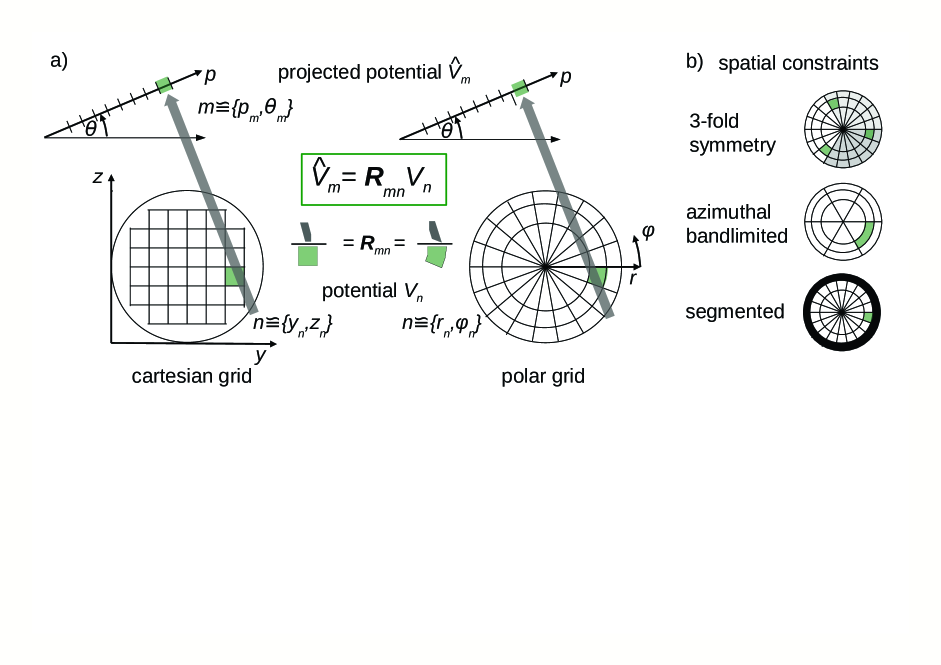
Figure 3: Algebraic tomography and sampling: a) A deliberately chosen sampling (left: Cartesian, right: polar) with sampling index $n$ is projected under a certain angle $\theta_{m}$ on the detector pixel $p_{m}$ with the projection weight of the reconstructed pixel $n$ determined by the normalized covering of the projection ray. b) Three examples of spatial constraints applied to the polar sampling scheme from top to bottom: 3-fold symmetric projection of 3 symmetric pixels into corresponding detector pixels; azimuthal band-limited projection facilitating reduction of azimuthal sampling points; deliberate exclusion of potential free region (e.g. vacuum) from Radon matrix.

For the (generalized) matrix inversion itself a large number of numerical methods has been developed. For tomography the Kaczmarz ($\cong$Algebraic Reconstruction Technique - ART) and related methods (e.g. Sequential Iterative Reconstruction Technique - SIRT) are very popular Natterer (2001), probably due to its particularly easy implementation and built-in quasi Tikhonov regularization parametrized by the number of iterations Hansen (1998). The latter refers to a a growing reconstruction of larger spatial frequency components at higher iteration numbers, implying a growth of spatial resolution at cost of increasing noise. However, the Kaczmarz method is not seeking for the optimal (fastest) iteration and is not optimized for sparse matrices such as the Radon matrix. Therefore, we use a conjugate gradient method implemented in the LSQR algorithm Paige and Saunders (1982) to reduce significantly the number of iterations (due to a weaker quasi Tikhonov regularization) and thus computing time.

II Results

We present results from a tomographic reconstruction incorporating a 3-fold symmetry constraint and 10 LSQR iterations on a $13800\times 11700$ Radon matrix for a polar grid. This choice is motivated by the good reconstruction quality (good spatial resolution at acceptable noise) containing all important potential features. We emphasize, however, that the regularization strength ($\cong$the number of iterations) can be deliberately varied; therefore we supplement reconstructions with 5 and 15 iterations and a reconstruction without symmetry constraint (see Supplementary Information). We furthermore note that a small charging of the NW could be observed through stray fields in the vacuum (see Fig. 1). Its influence on the reconstruction was tested to be around $0.1$ V by reconstructing with and without constraining the vacuum to $0$ V in the reconstruction. The reconstructed 3D potential of the GaAs-Al_0.33Ga_0.67As NW, which is illustrated by means of isosurfaces and $yz$-slices in Fig. 4b shows a slightly deformed 6-fold symmetry in the core-shell region corroborating the symmetry test performed on the projection data (Fig. 2b). We emphasize that due to the symmetry constraint missing wedge artifacts are now completely absent (see Wolf et al. (2011) for comparison); it would even be possible to use a trunctated tilt series interval of $60\text{\textdegree}$ here. In total, the achieved signal precision of about $0.2$ V (determined from the standard deviations of the corresponding homogeneous potential region along $x$) and spatial resolution of 6 nm (determined from the FWHM of the potential gradient at the NW boundary) is mainly limited by the holographic imaging process and not the EHT method; and therefore allows detecting the following features in 3D.

The Au NP at the NW tip has an average potential of $27.8\pm 0.2$ V (Fig. 4a,d) which agrees very well with the theoretical value of $28$ V obtained by multiplying the DFT value $30.1$ V Schowalter et al. (2006) with a dynamical scattering correction factor of $0.93$ Lubk et al. (2010). The same holds for the average potential of the GaAs core ($V_{\mathrm{exp}}=13.9\pm 0.1\,\mathrm{V},\,V_{\mathrm{theo}}=14.19\,\mathrm{V}$ Kruse et al. (2006)) and the Al_0.33Ga_0.67As shell ($V_{\mathrm{exp}}=13.4\pm 0.2\,\mathrm{V},\,V_{\mathrm{theo}}=0.33\cdot 12.34\,\mathrm{V}+0.67\cdot 14.19\,\mathrm{V}=13.58\,\mathrm{V}$ Kruse et al. (2006)). We furthermore observe an axial decay of the potential from the Au-Al_0.33Ga_0.67As interface over approximately $100$ nm comprising $0.5$ V (Fig. 4d), which could indicate a Fermi-Level-pinned Metal-AlGaAs junction or a varying chemical composition. In particular the appearance of a small potential ($V=12.5\pm 0.1\,\mathrm{V}$) region directly above the GaAs core (Fig. 4d) indicates the formation of a AlAs alloy reported for similar GaAs-Ga_cIn_1-cP core-shell NWs Sköld et al. (2005). The most remarkable features are characteristic 3-fold symmetric lines of reduced potential along {112}-directions of the NW (Fig. 4e). This observation is in striking agreement with the facet-dependent Al-segregation recently reported for this system Rudolph et al. (2013); Zheng et al. (2013), and ascribed to polarity-driven surface reconstruction during AlGaAs shell growth. Noteworthy, in Refs. Rudolph et al. (2013); Zheng et al. (2013) Al-enrichment along {112}-facets was detected in the shell by means of 2D cross-sectional STEM analysis and the determined Al concentration enhancement to $c_{Al}\approx 0.67$ agree with our value $c_{Al}=0.55\pm 0.5$ when taking into account a further increase at higher iteration numbers ($\cong$ higher spatial resolution, see Supplementary Information).

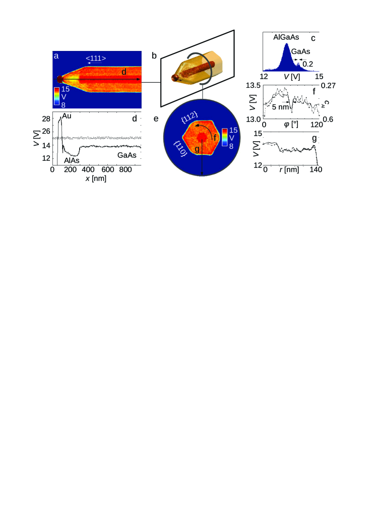
Figure 4: Reconstructed 3D potential of GaAs-Al_0.33Ga_0.67As core shell NW: The isosurfaces (b) at 9 and 13.75 V illustrate the core-shell morphology corroborated by the double peaks in the corresponding histogram (c). The $zx$-plane (a) with corresponding linescan (d) on the left shows the sequence Au, AlAs and GaAs unraveled through their different MIPs. The projected $yz$-plane (e) on the right with corresponding linescans in azimuthal (f) and radial (g) direction shows the core-shell structure with local Al accumulation identified through characteristic potential reduction in the azimuthal scan. Here, the corresponding Al concentration $c_{Al}$ determined from Vegard’s Law is shown on the right y-scale. The thick lines in (f) and (g) indicate averaged values from the whole hexagonal region of the NW.

A close inspection of the 3D potential additionally revealed fluctuations of the Al-enrichment around the above mean value. We ascribe them to modulations of the local faceting of the core as demonstrated in Fig. 5, where we show cross-sections from the unperturbed middle part (i.e. far away from the tapered region) of the NW. The depicted set of cross-sections clearly reveals a changing facet structure. Two effects can be distinguished. First there is a change in facet length, e.g. observable in the sequence $x=335\,\mathrm{nm}$ to $x=345.5$ nm. That effect has been reported in Ref. Johansson et al. (2007) and was there explained by alternating $\left\{111\right\}$-nanofacets accumulating to the six-fold $\left\{110\right\}$-facets observed on a larger length scale. Secondly, we observe a complete rotation of about $30\text{\textdegree}$ between $x=345.5\,\mathrm{nm}$ to $x=347.6$ possibly introduced by a twin boundary or a switch from $\left\{110\right\}$-facets to $\left\{112\right\}$-facets. These changes could be observed along the whole NW and are subjected to influence the growth of the shell structure in general and the Al-accumulation in particular.

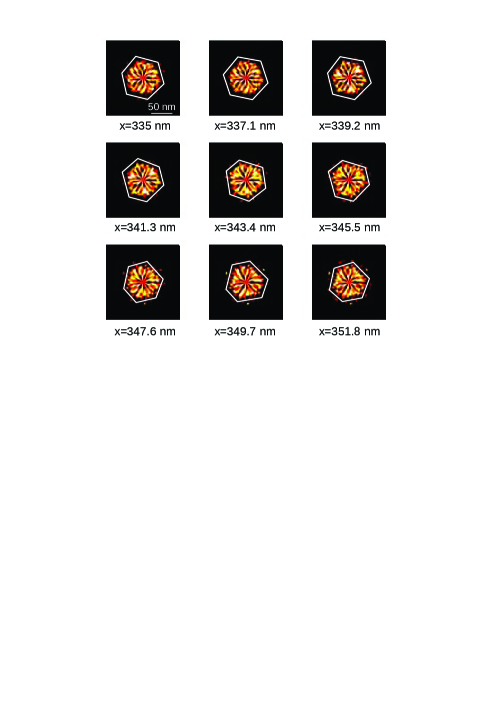
Figure 5: $\mathrm{GaAs}$-core showing a modulated facet structure. White frames are drawn around the core to indicate the core facets. The color range was restricted to an interval between 13.5 and 14.5 V to highlight the core region.

We again emphasize that the above features have been reconstructed in 3D for the first time (see Ref. Wolf et al. (2011) for comparison), i.e. quantitative compositional changes along $x$, $y$ and $z$ are revealed in parallel without the need to destructively prepare special cross-sections with possibly modified surfaces from the NW.

III Summary

In summary we demonstrated quantitative 3D electrostatic potential reconstruction with unprecedented accuracy and spatial resolution by a number of separate improvements implemented into electron holographic tomography (EHT). Most importantly, we developed automated acquisition and wave reconstruction schemes, procedures for 3D phase unwrapping, dynamic scattering correction, as well as optimal polar and symmetry adapted sampling. The latter two are beneficial to all tomographic techniques as a route towards faster and more accurate reconstructions. For the particular case of EHT our techniques facilitate reconstruction of nanoscale potentials such as originating from band bending or elemental segregation where spatial and signal resolution are critical. Similarly, 3D magnetic field reconstruction can be simplified by segmentation of the reconstruction volume into particle support and vacuum with the latter facilitating a reconstruction without the critical subtraction of the electrostatic phase shift.

IV Acknowledgments

AL, DW, and HL acknowledge financial support from the European Union under the Seventh Framework Programme under a contract for an Integrated Infrastructure Initiative. Reference 312483 - ESTEEM2. 8. SS is funded by the European Union (ERDF) and the Free State of Saxony via the ESF project 100087859 ENano. TN acknowledges financial support from the DFG within SFB 787 and INST 131/508-1.

References

- Radon (1917) J. Radon, Ber. Verh. Sächs. Akad. Wiss. Leipzig, Math. Nat. kl. 69, 262 (1917).
- Dunin-Borkowski et al. (2004) R. Dunin-Borkowski, M. McCartney, and D. Smith, in Encyclopedia of Nanoscience and Nanotechnology, edited by H. Nalwa (American Scientific Publishers, 2004), vol. 3, pp. 41–100.
- Lichte and Lehmann (2008) H. Lichte and M. Lehmann, Reports on Progress in Physics 71, 016102 (2008).
- Midgley and Dunin-Borkowski (2009) P. A. Midgley and R. E. Dunin-Borkowski, Nature materials 8, 271 (2009).
- Matteucci et al. (2002) G. Matteucci, G. Missiroli, and G. Pozzi, in Electron Microscopy and Holography II, edited by P. W. Hawkes (Elsevier, 2002), vol. Volume 122, pp. 173–249.
- Natterer (2001) F. Natterer, The mathematics of computerized tomography, vol. 32 of Classics in applied mathematics (Society for Industrial and Applied Mathematics, Philadelphia, 2001), ISBN 0898714931.
- Lai et al. (1994) G. Lai, T. Hirayama, K. Ishizuka, and A. Tonomura, Journal of Applied Optics 33, 829 (1994).
- Twitchett-Harrison et al. (2007) A. C. Twitchett-Harrison, T. J. V. Yates, S. B. Newcomb, R. E. Dunin-Borkowski, and P. A. Midgley, Nano Letters 7, 2020 (2007).
- Fujita and Chen (2009) T. Fujita and M. Chen, Journal of Electron Microscopy 58, 301 (2009).
- Wolf et al. (2010) D. Wolf, A. Lubk, H. Lichte, and H. Friedrich, Ultramicroscopy 110, 390 (2010).
- Midgley and Weyland (2003) P. A. Midgley and M. Weyland, Ultramicroscopy 96, 413 (2003).
- Tikhonov and Arsenin (1977) A. N. Tikhonov and V. Y. Arsenin, Solution of Ill-posed Problems. (Washington: Winston & Sons, 1977).
- Goris et al. (2012) B. Goris, W. Van den Broek, K. Batenburg, H. Heidari Mezerji, and S. Bals, Ultramicroscopy 113, 120 (2012).
- Batenburg et al. (2009) K. Batenburg, S. Bals, J. Sijbers, C. Kübel, P. Midgley, J. Hernandez, U. Kaiser, E. Encina, E. Coronado, and G. V. Tendeloo, Ultramicroscopy 109, 730 (2009).
- Hansen (1998) P. C. Hansen, Rank-Deficient and Discrete Ill-Posed Problems: Numerical Aspects of Linear Inversion (SIAM, Philadelphia,, 1998).
- Prete et al. (2008) P. Prete, F. Marzo, P. Paiano, N. Lovergine, G. Salviati, L. Lazzarini, and T. Sekiguchi, Journal of Crystal Growth 310, 5114 (2008).
- Wolf et al. (2011) D. Wolf, H. Lichte, G. Pozzi, P. Prete, and N. Lovergine, Applied Physics Letters 98, 264103 (pages 3) (2011).
- Rudolph et al. (2013) D. Rudolph, S. Funk, M. Doblinger, S. Morkötter, S. Hertenberger, L. Schweickert, J. Becker, S. Matich, M. Bichler, D. Spirkoska, et al., Nano Letters 13, 1522 (2013).
- Heiss et al. (2013) M. Heiss, Y. Fontana, A. Gustafsson, G. Wüst, C. Magen, D. D. O’Regan, J. W. Luo, B. Ketterer, S. Conesa-Boj, A. V. Kuhlmann, et al., Nature materials 12, 439 (2013).
- Bryllert et al. (2006) T. Bryllert, L.-E. Wernersson, T. Löwgren, and L. Samuelson, Nanotechnology 17, S227 (2006).
- Gallo et al. (2011) E. M. Gallo, G. Chen, M. Currie, T. McGuckin, P. Prete, N. Lovergine, B. Nabet, and J. E. Spanier, Applied Physics Letters 98, 241113 (2011).
- Krogstrup et al. (2013) P. Krogstrup, H. I. Jorgensen, M. Heiss, O. Demichel, J. V. Holm, M. Aagesen, J. Nygard, and A. Fontcuberta i Morral, Nat Photon 7, 306 (2013).
- Lehmann and Lichte (2002) M. Lehmann and H. Lichte, Microscopy and Microanalysis 8, 447 (2002).
- Ghiglia and Pritt (1998) D. C. Ghiglia and M. D. Pritt, Two-Dimensional Phase Unwrapping (Wiley, 1998).
- Lubk et al. (2010) A. Lubk, D. Wolf, and H. Lichte, Ultramicroscopy 110, 438 (2010).
- Gilbert (1972) P. Gilbert, Proc. R. Soc. Lond. B. 182, 89 (1972).
- Radermacher (2006) M. Radermacher, in Electron Tomography, Methods for Three-Dimensional Visualization of Structures in the Cell, edited by J. Frank (Springer, Berlin, 2006), pp. 245–274.
- Wolf et al. (2014) D. Wolf, A. Lubk, and H. Lichte, Ultramicroscopy 136, 15 (2014).
- Grillo and Rossi (2013) V. Grillo and F. Rossi, Ultramicroscopy 125, 112 (2013).
- Paige and Saunders (1982) C. C. Paige and M. A. Saunders, ACM Transactions on Mathematical Software 8, 195 (1982).
- Schowalter et al. (2006) M. Schowalter, A. Rosenauer, D. Lamoen, P. Kruse, and D. Gerthsen, Applied Physics Letters 88, 232108 (2006).
- Kruse et al. (2006) P. Kruse, M. Schowalter, D. Lamoen, A. Rosenauer, and D. Gerthsen, Ultramicroscopy 106, 105 (2006).
- Sköld et al. (2005) N. Sköld, L. S. Karlsson, M. W. Larsson, M.-E. Pistol, W. Seifert, J. Trägardh, and L. Samuelson, Nano Letters 5, 1943 (2005).
- Zheng et al. (2013) C. Zheng, J. Wong-Leung, Q. Gao, H. H. Tan, C. Jagadish, and J. Etheridge, Nano Lett. 13, 3742 (2013).
- Johansson et al. (2007) J. Johansson, L. S. Karlsson, C. P. T. Svensson, T. Mårtensson, B. A. Wacaser, K. Deppert, L. Samuelson, and W. Seifert, Journal of Crystal Growth 298, 635 (2007).