]Institute for Nonlinear Dynamics, University of Göttingen, Göttingen, Germany ]Lab. of Atomic & Solid-State Phys. and Sibley School of Mech. & Aerospace Eng., Cornell University, USA

Extreme fluctuations of the relative velocities between droplets in turbulent airflow

Abstract

We compare experiments and direct numerical simulations to evaluate the accuracy of the Stokes-drag model, which is used widely in studies of inertial particles in turbulence. We focus on statistics at the dissipation scale and on extreme values of relative particle velocities for moderately inertial particles ($St<1$). The probability distributions of relative velocities in the simulations were qualitatively similar to those in the experiments. The agreement improved with increasing Stokes number and decreasing relative velocity. Simulations underestimated the probability of extreme events, which suggests that the Stokes drag model misses important dynamics. Nevertheless, the scaling behavior of the extreme events in both the experiments and the simulations can be captured by the same multi-fractal model.

In warm clouds (with no ice), air-turbulence enhances the collision rate of the droplets. It thus influences the evolution of droplet sizes and the timescale for rain formation.Falkovich, Fouxon, and Stepanov (2002); Shaw (2003) Two mechanisms are at play: preferential concentration, due to a combination of dissipative dynamics and non-trivial correlations between the fluid flow and particle positions,Balkovsky, Falkovich, and Fouxon (2001); Bec et al. (2007); Saw et al. (2008) and very large approach velocities, explained in terms of the sling effectFalkovich, Fouxon, and Stepanov (2002); Bewley, Saw, and Bodenschatz (2013) and the formation of caustics.Wilkinson, Mehlig, and Bezuglyy (2006); Falkovich and Pumir (2007) Many questions remain open regarding the impact of such phenomena on the coalescence rate of droplets. Whilst it is generally accepted that turbulence increases droplet collision rates, too violent events can cause fragmentation.Orme (1997) To produce reliable models for coalescence efficiencies, a key issue is to understand how often this occurs. Such considerations are decisive for unravelling the impact of turbulence on the size distribution of droplets in clouds.

Contemporary theories and simulations of heavy particle dynamics in turbulent flows predominantly assume point particles coupled to the flow through linear Stokes drag. This simplification is justified when the particles are (a) smaller than the smallest scales of the flow, (b) made of material much denser than the fluid (i.e. heavy), and (c) far apart. Clearly the last premise fails when particles come close enough to collide and subject to mutual hydrodynamics interactions. In addition, several corrections to Stokes drag are missing from this framework and it is unclear when they are needed to capture the full dynamics. These include the Basset history force, nonlinear drag and the added mass effect. Recent studies suggest that the history force tends to suppress preferential concentration and caustic formation.Hill (2005); Daitche and Tél (2011) To find out the extent to which a model with Stokes drag alone is quantitatively descriptive, we compare experiments of droplets in turbulent air flow to results from direct numerical simulations (DNS) that match the conditions of the experiment, but with point particles coupled to the flow through Stokes drag. We then investigate the scaling of the particles’ relative velocities with respect to their spatial separation. This scaling is relevant for predicting collisional velocities at small scales from the large-scale statistics that are more easily measured. Finally, we compare our data with recent theoretical results and investigate the nature of the transition from tracer-like statistics at low relative velocities to the particle-inertia dominated statistics at large relative velocities.

The experiment is described in detail in Ref. Bewley, Saw, and Bodenschatz, 2013, and only an overview is given here. Nearly homogeneous and isotropic turbulent flows are generated in a $1\;m$-diameter acrylic sphere by 32 randomly pulsating jets. Each jet is made up of an audio-speaker capped by a conical nozzle.Chang, Bewley, and Bodenschatz (2012) The homogeneous and isotropic region was about $10\;cm$ in diameter and at the center of the apparatus. We ran the experiment under three different conditions, with the Taylor micro-scale Reynolds numbers, $R_{\lambda}$, being 160, 170 and 190 and kinetic energy dissipation rates ($\varepsilon$) $0.45\pm 0.05$, $1.2\pm 0.1$ and $3.2\pm 0.2\;m^{2}/s^{3}$, respectively (the corresponding Kolmogorov dissipative micro-scales, $\eta$, were 300, 230 and $180\;\mu m$). Droplets are produced with a spinning disc deviceWalton and Prewett (1949) that eject bi-disperse drops with diameters $6.8\mu m$ and 19$\mu m$ and standard deviations of $2\;\mu m$ and $4\;\mu m$, respectively. The Stokes numbers for the droplets are defined with respect to the Kolmogorov time-scale as $St=\tau_{\mathrm{p}}/\tau_{\eta}$ where $\tau_{\eta}=\sqrt{\nu/\varepsilon}$ is the Kolmogorov timescale and $\tau_{\mathrm{p}}=(2/9)(\rho_{\mathrm{p}}/\rho_{\mathrm{f}})a^{2}/\nu$ is the particle viscous response time ($\rho_{\mathrm{p}}$ and $\rho_{\mathrm{f}}$ are the particle and the fluid densities, respectively, $a$ the particle radius and $\nu$ the fluid kinematic viscosity). In order of increasing $R_{\lambda}$ for the flows studied, the large (small) droplets have Stokes number of values 0.19 (0.02), 0.31 (0.04) and 0.51 (0.06). Droplet motions are measured by imaging their shadows projected by white light sources into two cameras fitted with macro lenses, at a frame-rate of 15kHz ($>30/\tau_{\eta}$) and a spatial resolution of $3\;\mu m/pixel$ ($<\eta/50$, such unprecedented resolution allows us to measure the size and to distinguish the two groups of droplets). The 3D positions of droplets are determined by stereoscopic Lagrangian Particle Tracking.Ouellette et al. (2006)

The DNS are performed by using a pseudo-spectralGottlieb and Orszag (1977) parallel solver for the fluid velocity $\bm{u}$ obtained from the incompressible Navier–Stokes equation. Turbulence was sustained in a statistically stationary regime by holding constant the energy content of the lowest Fourier modes.Chen and Shan (1992) We use $512^{3}$ grid points with $\nu=1.5\times 10^{-4}$ (corresponding to $R_{\lambda}=180$) to approximately match the Reynolds numbers of the experiments. The droplets are approximated by individual point particles whose trajectories $\bm{X}(t)$ solve the Stokes equation

$$\ddot{\bm{X}}=-(1/\tau_{\mathrm{p}})\left[\dot{\bm{X}}-\bm{u}(\bm{X},t)\right]+\bm{g},$$ (1)

where the dots are time derivatives and $\bm{g}$ the acceleration of gravity. The fluid velocity at each particle position is obtained by cubic interpolation from the grid points. The point-particle approach (1) is expected to be valid when the particles size is much smaller than $\eta$ and their Reynolds number much less than unity. Furthermore, the particles in this model do not modify or perturb the flow, which may be valid when their volume fraction is small.

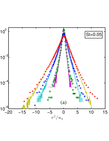
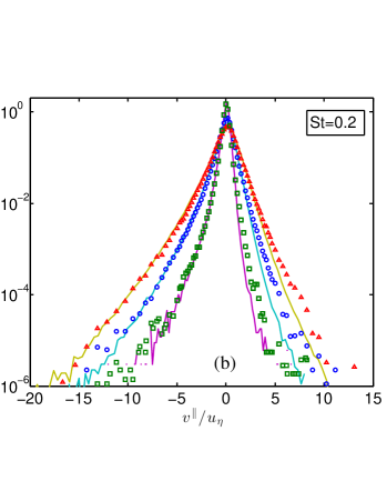
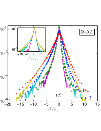
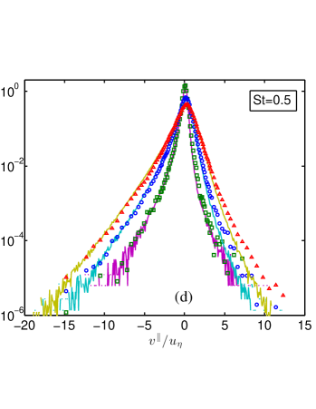
Figure 1: (Color online) PDF of the longitudinal velocity differences conditioned on different separations $r$ for (a) $St=0.05$, (b) $St=0.2$ , (c) $St=0.3$ and (d) $St=0.5$. Symbols are from experiments and solid lines from DNS. Squares/purple correspond to $r=1-1.6\eta$, circles/cyan to $r=3-3.6\eta$, and triangles/gold to $r=5-5.6\eta$. Note that unlike the DNS, the experimental droplets are not perfectly mono-disperse (details in text). Inset of (c): PDF for $r=1-1.6\eta$ and from bottom to top: $St=0.05$, $0.3$, $0.5$.

Of fundamental importance to the problem of turbulence-induced collisions between particles are the statistics of their longitudinal velocity difference $v^{\parallel}$ when the particles are close to each other. In Fig. 1 we show the probability density function (PDF) of $v^{\parallel}$ between two particles, conditioned on different values, $r$, of their separation. The plots are organized into four Stokes number groups: $St=0.05,0.2,0.3$ and $0.5$. For some of them, the experimental and simulated Stokes numbers slightly differ (for $St=0.05$, the experimental value is 0.04 and for $St=0.2$, the experimental and DNS values are 0.19 and 0.24 respectively). In the experiment the value of $R_{\lambda}$ changes a little between the various $St$ groups; thus minor Reynolds-number effect may be present. There is general agreement in the trends and shapes of the distributions. All can be approximated by stretched-exponentials whose concavity grows more pronounced with increasing $St$ and decreasing $r$. This is qualitatively consistent with what is known about the velocity distributions of fluid particles, which grow more stretched with decreasing scale.Kailasnath, Sreenivasan, and Stolovitzky (1992)

Both experiments and DNS show an increase in the amplitude of the left tail with increasing $St$, manifest in an increased skewness (more clearly in the inset of Fig. 1c). This implies that particles with larger inertia approach one another more violently on average than lighter ones. This is consistent with the sling effect, where inertial particles fly towards each other with relative velocities much higher than that of the background fluid, as explained in Ref. Gustavsson and Mehlig, 2011, 2013 and also observed in Ref. Bewley, Saw, and Bodenschatz, 2013. The faster approach should enhance their collision rate. Although similar skewness is well documented for fluid tracers, here we show that the skewness is further enhanced by particle inertia over the range of scales observed. The mechanism of this enhancement essentially involves occurrence of slings and subsequent damping by viscous drag. As seen in the inset, the advection dominated cores of the PDF do not change while the tails grow wider with increasing $St$, which makes the PDF more concave than that of fluid tracers. This observation is consistent with the existence of a velocity scale $\sim r/\tau_{\rm p}$ that separates the fluid-advection-dominated core of the PDFs from the inertia-dominated tails.Bewley, Saw, and Bodenschatz (2013)

Quantitatively, we found the differences between experiments and simulations to be less than about $15\%$ in the core of the distributions. Similarly, we found excellent agreement in the tails of the distributions, but only for the largest Stokes number ($St=0.5$), the smallest scale ($r<2\,\eta$), and for the left side of the distributions corresponding to approaching particle pairs. In other cases, the experimental tails of the PDFs increasingly deviate from the simulated ones as one moves to higher relative velocities. The discrepancy is larger in the right tails, corresponding to separating pairs, where in worst case the experimental data is about 5 times the DNS data. In the left tails, the discrepancy is less severe, but worsens with decreasing $St$, with the largest discrepancy at a factor of two.

In the case of $St=0.5$ (Fig. 1d), the discrepancy in the right tails seems at first glance to contradict the good agreement observed for the left tails. Here, effects beyond linear Stokes drag maybe at play (e.g., the Basset history force, the added mass and nonlinear drag forces). For example, there is some indication in recent numerical simulations that the history force plays an important role under some conditions.Daitche and Tél (2011) In any case, we could not find a clear explanation for the discrepancies, despite considering several possibilities including measurement uncertainty. To capture its influence, we characterized the measurement noise and added it to the DNS data. This however resulted only in a negligible widening of the tails of the distributions (the r.m.s. of the noise was in the data about $10\%$ of $v^{\parallel}$ ). We also evaluated the accuracy of the method used to estimate $\varepsilon$, in the experiment by applying the same method to the DNS data i.e., by using $\left\langle[v^{\parallel}]^{2}\right\rangle=\varepsilon\,r^{2}/(15\nu)$ for $r<5\eta$ and on particles of $St=0.05$). This resulted in very good agreement (within 5%) with the direct measure of $\varepsilon$ in DNS, and so gave a strong support to the $\varepsilon$ reported in the experiment. We checked that Reynolds number effect could not account for the discrepancies by comparing DNS data at increasing Reynolds numbers (up to $R_{\lambda}=287$). This addressed partially the question of small scale universality of the turbulence statistics in the flows studied. We also explored the possibility of inaccuracy of $\nu$ in the experiment by reprocessing the experimental data with a modified $\nu$ ($\pm 30\%$) and found no clear improvement. The droplets’ Reynolds numbers ($u_{\eta}a/\nu$) were of the order of 0.1 on average, so that the effect of non-linear drag on the droplets were typically negligible. We note that given the conditions of our experiment, and specifically since $a/\eta$ was of the order of 0.1, the history force term stands next to the Stokes drag in the hierarchy of importance amongst the various forces on the droplets.Maxey and Riley (1983) In summary, the influences of nonlinear forces, hydrodynamic interactions, and non-universal turbulence statistics merit further study.

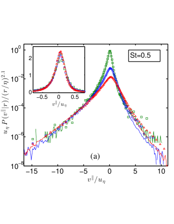
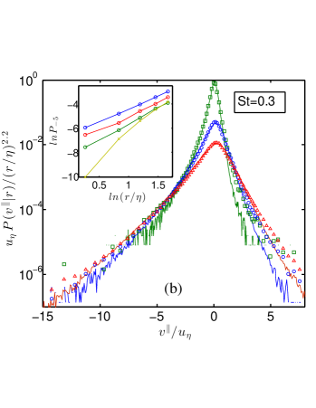
Figure 2: (Color online) (a) Rescaled PDFs of the longitudinal velocity difference from the experiment (symbols) and the DNS (solid lines) for $St=0.5$, with $\beta$ = 2.1, and different separations: $r=1-1.6\eta$ (green), $r=3-3.6\eta$ (blue), and $r=5-5.6\eta$ (red). Inset: PDF of $\tau_{\eta}v^{\parallel}/r$ showing the $r$-scaling of the distribution bulk. (b) Same as (a) for $St=0.3$ with $\beta$ = 2.2. Inset: plots of $lnP_{-5}=\ln[\mathrm{Pr}\,(v^{\parallel}/u_{\eta}<5\,|r)]$ for $St$ = 0.5 (blue), 0.3 (red), 0.2 (green) and 0.04 (gold crosses). The values of $\beta$ were obtained as the linear slope of each of these curves, namely $\beta_{St=0.5}=2.1$, $\beta_{St=0.3}=2.2$ and $\beta_{St=0.2}=2.7$. Unambiguous values of $\beta$ could not be obtained for $St=0.04$.

The problem of droplet collision-coalescence in clouds involves droplet relative velocities at contact, which is typically of the order of 100 times smaller than $\eta$. To that end, it is of interest to understand how droplet relative velocities scale with vanishing $r$ (granted that other inter-particle forces at small scales will need to be accounted for a full description). Figure 2(a) presents the PDF of $v^{\parallel}$ conditioned on different values of $r$ for $St=0.5$. We find that both the experimental and DNS data collapse at large negative values of $v^{\parallel}$ when the PDF is rescaled by $r^{\beta}$ with $\beta\approx 2.1$. Similar analysis for the case of $St=0.3$ is shown in Figure 2(b). Such collapse indicates that the distribution of violent approaching velocities takes the form $p(v^{\parallel}\,|\,r)\simeq r^{\beta(St)}\,\phi(v^{\parallel})$ at sufficiently small separations and large velocities.Gustavsson and Mehlig (2013) It is straightforward to show analyticallyCelani et al. (2000) that the exponent $\beta$ corresponds exactly to the saturated value $\xi_{\infty}$ of the scaling exponents of the structure functions of particle relative velocities in the limit of large orderBec et al. (2010) (i.e., $\langle|v^{\parallel}|^{p}\,|\,r\rangle\propto r^{\xi_{p}}$ with $\xi_{p}=\xi_{\infty}$ for all sufficiently large $p$). The collapse to a scale-independent form occurs for large velocity differences, namely $|v^{\parallel}|\gg r/\tau_{\mathrm{p}}$. This condition corresponds to a traveling time over a distance $r$ that is much shorter than the particle response time, so that damping is negligible. Under these conditions particle pairs move ballistically, which is related to the sling effect.Falkovich, Fouxon, and Stepanov (2002); Bewley, Saw, and Bodenschatz (2013); Gustavsson and Mehlig (2011, 2013) Gustavsson and MehligGustavsson and Mehlig (2011, 2013) predict that $\xi_{\infty}=3-D_{2}\equiv c_{1}$, where $D_{2}$ is the fractal (correlation) dimension of inertial particle clusters and $c_{1}$ the corresponding exponent of the radial distribution function. In the case of $St=0.5$, $\xi_{\infty}\simeq 0.7$ using value of $c_{1}$ from e.g. Ref. Saw et al., 2012. Our measured value $\xi_{\infty}(St=0.5)\simeq 2.1$ differs from the prediction; this deviation could however disappear at much smaller $r$-scales.

By using matched asymptotics techniques, Gustavsson and MehligGustavsson and Mehlig (2011, 2013) proposed to approximate the scaling exponents $\xi_{p}$ of relative velocities as

$$\xi_{p}=p\quad\mbox{for}\ p\leq\xi_{\infty}\qquad\mbox{and}\qquad\xi_{p}=\xi_{\infty}\quad\mbox{for}\ p>\xi_{\infty}.$$ (2)

Thence in the limit of small $r/\eta$, the core of the PDF of $v^{\parallel}$ inherits the scaling of the fluid tracers, namely $p(v^{\parallel}|r)\sim r^{-1}\,\psi(v^{\parallel}/r)$, with a transition at $|v^{\parallel}|\propto r/\tau_{p}$ to a scaling in the tails of the form $p(v^{\parallel}|r)\sim r^{\,\xi_{\infty}}\,\Phi(v^{\parallel})$ which we discussed above. The behavior (2) pertains to bi-fractal statistics. As illustrated in Figs. 3a and b, this is a special case of multi-fractal statistics, which are ubiquitous in turbulence.Frisch (1996) For the problem of droplet collisions in clouds, which depends on the first moments of the relative particle velocity and concerns the moderate $St$ studied here, distinguishing between the two possibilities is of consequence, since this is where the difference between the two is most significant.

Our data are consistent with the bifractal picture given above for both asymptotically large and small $v^{\parallel}$, as shown in the main plot of Fig. 2 for the scaling of the tail and in the inset for the scaling of the core. However, the behavior in the transition range ($|v^{\parallel}|\approx r/\tau_{p}$) differentiates a bifractal from a multifractal, and the sharpness of the transition is hard to judge from this figure. Hence we take a different approach as shown below.

Multifractal analysis emerged in the context of strange attractorsPaladin and Vulpiani (1987) and of the anomalous scaling observed for inertial-range statistics in turbulence.Frisch (1996) Typical methods rely on box-counting, or on evaluating moments and scaling exponents.Meneveau and Sreenivasan (1991) In the specific case of inertial-particle velocity differences in the dissipation range, measuring the scaling exponents $\xi_{p}$ as a function of $p$ is particularly difficult as it relies on fitting data to power-laws at scales where statistics deteriorate. For that reason, we use here the interpretation of multifractal statistics in terms of the theory of large deviations.Broniatowski and Mignot (2001) We assume a continuum of local scaling exponents $h=\ln|v^{\parallel}/v_{\ell}|/\ln(r/\ell)$, where $\ell$ is a typical length of convergence to the scaling regime and $v_{\ell}$ the associated velocity. In the asymptotics $r\ll\ell$, the probability density of $h$ reads $p(h\,|\,r)\sim(r/\ell)^{S(h)}$, where $S(h)$ is the rate function (furthermore, $S(h)=3-D(h)$, where $D(h)$ is the multifractal spectrum, that is the dimension of the set of points where $v^{\parallel}\sim r^{h}$). The scaling exponents trivially relate to the rate function by a Legendre transform $\xi_{p}=\inf_{h}[ph+S(h)]$. Typical behaviors of $\xi_{p}$ and $S(h)$ are sketched in Fig. 3a and b. For tracers, dissipation-range velocity differences are given by $v^{\parallel}=r\,\partial_{r}u$, where $\partial_{r}u$ is the radial fluid velocity gradient. This leads to $\xi_{p}=p$ and $S(h)=h-1$ for $h\geq 1$, and $S(h)=\infty$ otherwise. For bifractal statistics, $\xi_{p}=\min(p,\xi_{\infty})$ and $S(h)=h-1$ for $h\geq 1$, and $S(h)$ is a concave function for $h<1$. In the multifractal case there must be no sharp transition at any $p$ or $h$ and $S(h)$ is a convex function around its minimum. Distinguishing between bifractal and multifractal statistics can thus be recast as an investigation into whether $S(h)$ is convex or concave near its minimum.

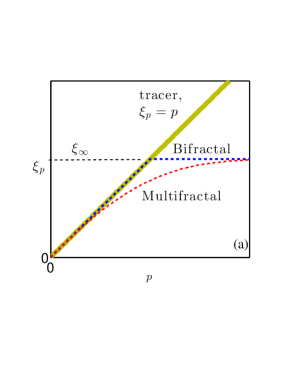
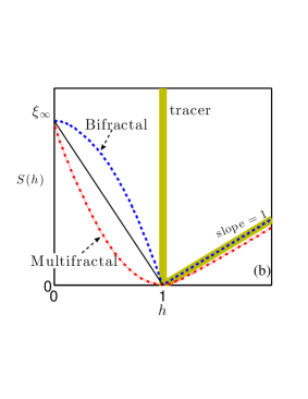
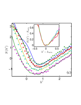
Figure 3: (Color online) (a) and (b): Schematic representation of the main features of multi-fractal and bi-fractal statistics and the behaviors expected for fluid tracers in the dissipative scales of turbulent flows. (a) Scaling exponent $\xi_{p}$ (such that $\langle|v^{\parallel}|^{p}\,|\,r\rangle\propto r^{\xi_{p}}$). (b) Corresponding rate functions $S(h)$ (see text for details). (c) Rate function, $S(h)$, in the case of $St=0.5$ for the experiment (markers) and the DNS (solid lines) and various separations. $S(h)$ was calculated using $S(h)=\ln[p(h\,|\,r_{2})/p(h\,|\,r_{1})]/\ln(r_{2}/r_{1})$, where the $r_{i}$’s are the middle values of the $r$-bins with width $\Delta r=0.6\eta$. From the bottom curve to the top, the values of $(r_{1}/\eta,r_{2}/\eta)$ were respectively (1.3, 2.3), (2.3, 3.3), (3.3, 4.3) and (4.3, 5.3). Inset: Shifted $S(h)$ at smaller $r$’s using the DNS data. All curves are linearly shifted such that their minimum is at $(0,1)$. Collapse implies that the limiting form is reached at these $r$ values which are, in the order red-cyan-purple-gold, respectively: $(r_{1}/\eta,r_{2}/\eta)=$(0.15, 0.45), (0.45, 0.75), (0.75, 1.05), (1.05, 1.35), with bin widths of $\Delta r=0.3\eta$.

The measurement of $h$ and of $S(h)$ requires some attention because their definitions include the undetermined scales $\ell$ and $v_{\ell}$. Particular definitions of $\ell$ and $v_{\ell}$ do not alter the values of $h$ and $S(h)$ in the limit $r\to 0$, but we cannot reach this limit in practice. The explicit dependence of $S(h)$ on $\ell$ and $v_{\ell}$ can be eliminated by using the formula $\ln[p(h\,|\,r_{2})/p(h\,|\,r_{1})]/\ln(r_{2}/r_{1})$. There is however no such stratagem to make $h$ independent of $\ell$ and $v_{\ell}$. A given choice, say $\ell^{\prime}$ and $u_{\ell}^{\prime}$, leads to a measurement of the scaling exponent $h^{\prime}=\ln|v^{\parallel}/v_{\ell}^{\prime}|/\ln(r/\ell^{\prime})$ that for any finite $r$ differs from reference choices of $\ell$ and $v_{\ell}$ by $h^{\prime}=h+[h\ln(\ell/\ell^{\prime})+\ln(v_{\ell}/v_{\ell}^{\prime})]/\ln(r/\ell^{\prime})$. Thus, we must choose definitions for $\ell^{\prime}$ and $u_{\ell}^{\prime}$.

The main panel of Fig. 3c shows $S(h^{\prime})$ obtained from our experiments and DNS for $\ell^{\prime}=10\eta$ and $u_{\ell}^{\prime}=u_{\eta}$, and with $r$ going from $\simeq 5\eta\text{ to }\eta$. The $y$-axis intercept for the case of $r\simeq\eta$, albeit noisy, gives roughly the value deduced from Fig. 2, namely $\xi_{\infty}\approx 2.1$. The location of the minimum shifts towards $(1,0)$ as $r$ decreases. The vertical displacement is partly due to the normalization factor present in $p(h\,|\,r)$, which itself involves some $r$ dependence,van de Water and Schram (1988) and can be compensated by subtracting from $S(h^{\prime})$ the value $S_{\min}=S(h^{\prime}_{\min})$ of its minimum. The origin of the horizontal displacement can be twofold: it is either due to finite-$r$ deviations from the limiting form of $S(h)$ or to a mismatch in the definition of $h^{\prime}$ due to our arbitrary choice of $\ell^{\prime}$ and $v_{\ell}^{\prime}$. The DNS data were consistent with $h^{\prime}_{\min}\simeq 1+C/\ln(r/\ell^{\prime})$, giving a strong support to the second scenario.

In order to probe the limiting form of $S$ close to its minimum at vanishing $r$, we show in the inset of Fig. 3c the rate functions $S(h)$ from the DNS with their minima translated to $(0,0)$, for $r\simeq 0.15\eta$ to $1.05\eta$. The excellent collapse of these curves around their minima suggests that they have reached their final limiting form at $r\lesssim\eta$. The frozen curvature around the minimum, for about a decade in $r$, indicates that $S(h)$ is convex and thus supports the view that the statistics are multi-fractal, and not bifractal. However, we cannot rule out that this is an intermediate regime and that bi-fractality could be recovered at even smaller separations.

To summarize, we evaluated the accuracy of the Stokes drag model for the advection of inertial particles in turbulent flow by comparing the results from DNS with experimental measurements. Focussing on large (longitudinal) relative velocities, we found that DNS reproduced all qualitative trends of the experiments. Furthermore, accurate quantitative agreements were found for inertia-dominated regimes ($St=0.5$, $v^{\parallel}\lesssim-r/\tau_{\mathrm{p}}$). Discrepancies up to a factor of 5 were found for regimes less influenced by particle inertia (that is, for separating particles or for small $St$). Further analysis did not support trivial explanations for such discrepancies, which implies that the discrepancies could have been caused either by corrections to the Stokes drag model, such as the Basset history force or hydrodynamic interactions between particles, or by small-scale non-universality of the turbulence (DNS and experiment have different large scale energy injection schemes). Where the data agree, they consistently show that for inertial particles and at dissipative scales of turbulence, the tails of the probability density function of $v^{\parallel}$ scale as a power law of $r$. This is consistent with the saturation of the scaling exponents of the moments of velocities differences found in previous studies. Furthermore, the frozen convexity of the rate function, $S(h)$, at small $r$ is consistent with multi-fractal statistics of velocities differences.

Several questions remain open. Foremost there is a clear need to resolve the velocity difference statistics at very small particle separations, in order to assess the recent theories (Ref. Gustavsson and Mehlig, 2011, 2013). Also, very little is known about the effect of turbulent intermittency on the statistics of caustics; this could lead to non-trivial Reynolds number dependencies of particle relative velocity and collision statistics. This would, for instance, make it possible to disentangle Reynolds number effects from Stokes number effects. These questions will be addressed in future work.

We acknowledge Poh Yee Lim for help with the experiments; Holger Homann for help with the simulation; M. Cencini, B. Mehlig and S. Musacchio for crucial discussions. This work received funding from the Max Planck Society (Germany) and the European Research Council under the European Community’s Seventh Framework Program (FP7/2007-2013, Grant Agreement no. 240579). SSR acknowledges the support of the Indo-French Center for Applied Mathematics (IFCAM) and from the AIRBUS Group Corporate Foundation Chair in Mathematics of Complex Systems established in ICTS. Computations were performed on the IBM Blue Gene/P computer JUGENE at the FZ Jülich was made available through the PRACE project PRA031 and on the “mésocentre de calcul SIGAMM”.

References

- Falkovich, Fouxon, and Stepanov (2002) G. Falkovich, A. Fouxon, and M. Stepanov, “Acceleration of rain initiation by cloud turbulence,” Nature 419, 151–154 (2002).
- Shaw (2003) R. Shaw, “Particle-turbulence interactions in atmospheric clouds,” Ann. Rev. Fluid Mech. 35, 183–227 (2003).
- Balkovsky, Falkovich, and Fouxon (2001) E. Balkovsky, G. Falkovich, and A. Fouxon, “Intermittent distribution of inertial particles in turbulent flows,” Phys. Rev. Lett. 86, 2790–2793 (2001).
- Bec et al. (2007) J. Bec, L. Biferale, M. Cencini, A. Lanotte, S. Musacchio, and F. Toschi, “Heavy particle concentration in turbulence at dissipative and inertial scales,” Phys. Rev. Lett. 98, 84502 (2007).
- Saw et al. (2008) E.-W. Saw, R. A. Shaw, S. Ayyalasomayajula, P. Y. Chuang, and A. Gylfason, “Inertial clustering of particles in high-reynolds-number turbulence,” Phys. Rev. Lett. 100, 214501 (2008).
- Bewley, Saw, and Bodenschatz (2013) G. P. Bewley, E.-W. Saw, and E. Bodenschatz, “Observation of the sling effect,” New J. Phys. 15, 083051 (2013).
- Wilkinson, Mehlig, and Bezuglyy (2006) M. Wilkinson, B. Mehlig, and V. Bezuglyy, “Caustic activation of rain showers,” Phys. Rev. Lett. 97, 48501 (2006).
- Falkovich and Pumir (2007) G. Falkovich and A. Pumir, “Sling effect in collisions of water droplets in turbulent clouds,” J. Atmos. Sci. 64, 4497–4505 (2007).
- Orme (1997) M. Orme, “Experiments on droplet collisions, bounce, coalescence and disruption,” Prog. Energy Combust. Sci. 23, 65–79 (1997).
- Hill (2005) R. J. Hill, “Geometric collision rates and trajectories of cloud droplets falling into a burgers vortex,” Phys. Fluids 17, 037103 (2005).
- Daitche and Tél (2011) A. Daitche and T. Tél, “Memory effects are relevant for chaotic advection of inertial particles,” Phys. Rev. Lett. 107, 244501 (2011).
- Chang, Bewley, and Bodenschatz (2012) K. Chang, G. P. Bewley, and E. Bodenschatz, “Experimental study of the influence of anisotropy on the inertial scales of turbulence,” J. Fluid Mech. 692, 464 (2012).
- Walton and Prewett (1949) W. H. Walton and W. C. Prewett, “The production of sprays and mists of uniform drop size by means of spinning disc type sprayers,” Proc. Phys. Soc. B 62, 341–350 (1949).
- Ouellette et al. (2006) N. Ouellette, H. Xu, M. Bourgoin, and E. Bodenschatz, “An experimental study of turbulent relative dispersion models,” New J. Phys. 8, 109 (2006).
- Gottlieb and Orszag (1977) D. Gottlieb and S. A. Orszag, Numerical analysis of spectral methods, Vol. 2 (SIAM, 1977).
- Chen and Shan (1992) S. Chen and X. Shan, “High-resolution turbulent simulations using the connection machine-2,” Comput. in Phys. 6, 643–646 (1992).
- Kailasnath, Sreenivasan, and Stolovitzky (1992) P. Kailasnath, K. Sreenivasan, and G. Stolovitzky, “Probability density of velocity increments in turbulent flows,” Phys. Rev. Lett. 68, 2766–2769 (1992).
- Gustavsson and Mehlig (2011) K. Gustavsson and B. Mehlig, “Distribution of relative velocities in turbulent aerosols,” Phys. Rev. E 84, 045304 (2011).
- Gustavsson and Mehlig (2013) K. Gustavsson and B. Mehlig, “Relative velocities of inertial particles in turbulent aerosols,” J. Turbul. 15, 34–69 (2013).
- Maxey and Riley (1983) M. R. Maxey and J. J. Riley, “Equation of motion for a small rigid sphere in a nonuniform flow,” Phys. Fluids 26, 883–889 (1983).
- Celani et al. (2000) A. Celani, A. Lanotte, A. Mazzino, and M. Vergassola, “Universality and saturation of intermittency in passive scalar turbulence,” Phys. Rev. Lett. 84, 2385 (2000).
- Bec et al. (2010) J. Bec, L. Biferale, M. Cencini, A. Lanotte, and F. Toschi, “Intermittency in the velocity distribution of heavy particles in turbulence,” J. Fluid Mech. 646, 527–536 (2010).
- Saw et al. (2012) E.-W. Saw, J. P. Salazar, L. R. Collins, and R. A. Shaw, “Spatial clustering of polydisperse inertial particles in turbulence: I. comparing simulation with theory,” New J. Phys. 14, 105030 (2012).
- Frisch (1996) U. Frisch, Turbulence (Cambridge University Press, Cambridge, UK, 1996).
- Paladin and Vulpiani (1987) G. Paladin and A. Vulpiani, “Anomalous scaling laws in multifractal objects,” Phys. Rep. 156, 147–225 (1987).
- Meneveau and Sreenivasan (1991) C. Meneveau and K. Sreenivasan, “The multifractal nature of turbulent energy dissipation,” J. Fluid Mech. 224, 429–484 (1991).
- Broniatowski and Mignot (2001) M. Broniatowski and P. Mignot, “A self-adaptive technique for the estimation of the multifractal spectrum,” Stat. & Prob. Lett. 54, 125–135 (2001).
- van de Water and Schram (1988) W. van de Water and P. Schram, “Generalized dimensions from near-neighbor information,” Phys. Rev. A 37, 3118 (1988).