Triadic closure as a basic generating mechanism of communities in complex networks

Abstract

Most of the complex social, technological and biological networks have a significant community structure. Therefore the community structure of complex networks has to be considered as a universal property, together with the much explored small-world and scale-free properties of these networks. Despite the large interest in characterizing the community structures of real networks, not enough attention has been devoted to the detection of universal mechanisms able to spontaneously generate networks with communities. Triadic closure is a natural mechanism to make new connections, especially in social networks. Here we show that models of network growth based on simple triadic closure naturally lead to the emergence of community structure, together with fat-tailed distributions of node degree, high clustering coefficients. Communities emerge from the initial stochastic heterogeneity in the concentration of links, followed by a cycle of growth and fragmentation. Communities are the more pronounced, the sparser the graph, and disappear for high values of link density and randomness in the attachment procedure. By introducing a fitness-based link attractivity for the nodes, we find a novel phase transition, where communities disappear for high heterogeneity of the fitness distribution, but a new mesoscopic organization of the nodes emerges, with groups of nodes being shared between just a few superhubs, which attract most of the links of the system.

I Introduction

Complex networks are characterized by a number of general properties, that link together systems of very diverse origin, from nature, society and technology Albert and Barabási (2002); Barrat et al. (2008); Newman (2010). The feature that has received most attention in the literature is the distribution of the number of neighbors of a node (degree), which is highly skewed, with a tail that can be often well approximated by a power law Albert et al. (1999). Such property explains a number of striking characteristics of complex networks, like their high resilience to random failures Albert et al. (2000) and the very rapid dynamics of diffusion phenomena, like epidemic spreading Pastor-Satorras and Vespignani (2001). The generally accepted mechanism yielding broad degree distributions is preferential attachment Barabási and Albert (1999): in a growing network, new nodes set links with existing nodes with a probability proportional to the degree of the latter. This way the rate of accretion of neighbors will be higher for nodes with more connections, and the final degrees will be distributed according to a power law. Such basic mechanism, however, taken alone without considering additional growing rules, generates networks with very low values of the clustering coefficient, a relevant feature of real networks Watts and Strogatz (1998). Furthermore, these networks have no community structure Girvan and Newman (2002); Fortunato (2010) either.

High clustering coefficients imply a high proportion of triads (triangles) in the network. It has been pointed out that there is a close relationship between a high density of triads and the existence of community structure, especially in social networks, where the density of triads is remarkably high Newman and Park (2003); Newman (2003); Toivonen et al. (2006); Kumpula et al. (2007); Foster et al. (2011). Indeed, if we stick to the usual concept of communities as subgraphs with an appreciably higher density of (internal) links than in the whole graph, one would expect that triads are formed more frequently between nodes of the same group, than between nodes of different groups Granovetter (1973). This concept has been actually used to implement well known community finding methods Palla et al. (2005); Radicchi et al. (2004). Foster et al. Foster et al. (2011) have studied equilibrium graph ensembles obtained by rewiring links of several real networks such to preserve their degree sequences and introduce tunable values of the average clustering coefficient and degree assortativity. They found that the modularity of the resulting networks is the more pronounced, the larger the value of the clustering coefficient. Correlation, however, does not imply causation, and the work does not provide a dynamic mechanism explaining the emergence of high clustering and community structure.

Triadic closure Rapoport (1953) is a strong candidate mechanism for the creation of links in networks, especially social networks. Acquaintances are frequently made via intermediate individuals who know both us and the new friends. Besides, such process has the additional advantage of not depending on the features of the nodes that get attached. With preferential attachment, it is the node’s degree that determine the probability of linking, implying that each new node knows this information about all other nodes, which is not realistic. Instead, triadic closure induces an effective preferential attachment: getting linked to a neighbor $A$ of a node corresponds to choosing $A$ with a probability increasing with the degree $k_{A}$ of that node, according to a linear or sublinear preferential attachment. This principle is at the basis of several generative network models Holme and Kim (2002); Davidsen et al. (2002); Vázquez (2003); Marsili et al. (2004); Toivonen et al. (2006); Jackson and Rogers (2007); Solé et al. (2002); Krapivsky and Redner (2005); Ispolatov et al. (2005); Lambiotte ; Aynaud et al. (2013), all yielding graphs with fat-tailed degree distributions and high clustering coefficients, as desired. Toivonen et al. have found that community structure emerges as well Toivonen et al. (2006).

Here we propose a first systematic analysis of models based on triadic closure, and demonstrate that this basic mechanism can indeed endow the resulting graphs with all basic properties of real networks, including a significant community structure. These models can include or not an explicit preferential attachment, they can be even temporal networks, but as long as triadic closure is included, the networks are sufficiently sparse, and the growth is random, a significant community structure spontaneously emerges in the networks. In fact the nodes of these networks are not assigned any “ a priori” hidden variable that correlates with the community structure of the networks.

We will first discuss a basic model including triadic closure but not an explicit preferential attachment mechanism and we will characterize the community formation and evolution as a function of the main variables of the linking mechanism, i.e. the relative importance of closing a triad versus random attachment and the average degree of the graph. We find that communities emerge when there is a high propensity for triadic closure and when the network is sufficiently sparse (low average degree). We will also consider further models existing in the literature and including triadic closure, and we show that results concerning the emergence of the community structure are qualitatively the same, independently on the presence or not of the explicit preferential attachment mechanism or on the temporal dynamics of the links. Finally, we will introduce a variant of the basic model, in which nodes have a fitness and a propensity to attract new links depending on their fitness. Here clusters are less pronounced and, when the fitness distribution is sufficiently skewed, they disappear altogether, while new peculiar aggregations of the nodes emerge, where all nodes of each group are attached to a few superhubs.

II The basic model including triadic closure

We begin with what is possibly the simplest model of network growth based on triadic closure. The starting point is a small connected network of $n_{0}$ nodes and $m_{0}\geq m$ links. The basic model contains two ingredients:

• Growth. At each time a new node is added to the network with $m$ links.

• Proximity bias. The probability to attach the new node to node $i$ depends on the order in which the links are added.
  The first link of the new node is attached to a random node $i_{1}$ of the network. The probability that the new node is attached to node $i_{1}$ is then given by

  $$\Pi^{[0]}(i_{1})=\frac{1}{n_{0}+t}\,.$$ (1)

  The second link is attached to a random node of the network with probability $1-p$, while with probability $p$ it is attached to a node chosen randomly among the neighbors of node $i_{1}$. Therefore in the first case the probability to attach to a node $i_{2}\neq i_{1}$ is given by

  $$\Pi^{[0]}(i_{2})=\frac{(1-\delta_{i_{1},,i_{2}})}{n_{0}+t-1}\,,$$ (2)

  where $\delta_{i_{1},i_{2}}$ indicates the Kronecker delta, while in the second case the probability $\Pi^{[1]}(i_{2})$ that the new node links to node $i_{2}$ is given by

  $$\Pi^{[1]}({i_{2}})=\frac{a_{i_{1},i_{2}}}{k_{i_{1}}}\,,$$ (3)

  where $a_{ij}$ is the adjacency matrix of the network and $k_{i1}$ is the degree of node $i_{1}$.

• Further edges. For the model with $m>2$, further edges are added according to the “second link” rule in the previous point. With probability $p$, and edge is added to a random neighbor without a link of the first node $i_{1}$. With probability $1-p$, a link is attached to a random node in the network without a link already. A total of $m$ edges are added, $1$ initial random edge and $m-1$ involving triadic closure or random attachment.

In Fig. 1 the attachment mechanism of the model is schematically illustrated.

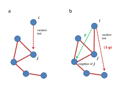
Figure 1: (Color online) Basic model. One link associated to a new node $i$ is attached to a randomly chosen node $j$, the other links are attached to neighbors of $j$ with probability $p$, closing triangles, or to other randomly chosen nodes with probability $1-p$.

For simplicity we discuss here the case $m=2$. In the basic model the probability that a node $i$ acquires a new link at time $t$ is given by

$$\frac{1}{t}\left[(2-p)+p\sum_{j}\frac{a_{ij}}{k_{j}}\right].$$ (4)

In an uncorrelated network, where the probability $p_{ij}$ that a node $i$ is connected to a node $j$ is $p_{ij}=\frac{k_{i}k_{j}}{\langle{k}\rangle n}$ ($n$ being the number of nodes of the network), we might expect that the proximity bias always induces a linear preferential attachment, i.e.

$$\sum_{j}\frac{a_{ij}}{k_{j}}\propto k_{i},$$ (5)

but for a correlated network this guess might not be correct. Therefore, assuming, as supported by the simulation results (see Fig.  2), that the proximity bias induces a linear or sublinear preferential attachment, i.e.

$$\Theta_{i}=p\sum_{j}\frac{a_{ij}}{k_{j}}\simeq ck_{i}^{\theta},$$ (6)

with $\theta=\theta(p)\leq 1$ and $c=c(p)$, we can write the master equation Mendes and Dorogovtsev (2003) for the average number $n_{k}(t)$ of nodes of degree $k$ at time $t$. from the simulation results it is found that the function $\theta(p)$ is an increasing function of $p$ for $m=2$. Moreover the exponent $theta$ is also an increasing function of the number of edges of the new node $m$. Assuming the scaling in Eq. $(\ref{Theta})$, the master equation for $m=2$ reads

$$n_{k}(t+1) = n_{k}(t)+\frac{2-p+c(k-1)^{\theta}}{t}n_{k-1}(t)(1-\delta_{k,2})$$ (7)

$$-\frac{2-p+ck^{\theta}}{t}n_{k}(t)+\delta_{k,2}.$$

In the limit of large values of $t$, we assume that the degree distribution $P(k)$ can be found as $n_{k}/t\to P(k)$. So we find the solution for $P(k)$

$$P(k)=C\frac{1}{3-p+ck^{\theta}}\prod_{j=1}^{k-1}\left(1-\frac{1}{3-p+cj^{\theta}}\right)\,,$$ (8)

where $C$ is a normalization factor. This expression for $\theta<1$ can be approximated in the continuous limit by

$$P(k)\simeq D\frac{1}{3-p+ck^{\theta}}e^{-(k-1)G(k-1,\theta,c)}\,,$$ (9)

where $D$ is the normalization constant and $G(k,\theta,c)$ is given by

$$G(k,\theta,c) = -\theta\ {{}_{2}F_{1}}\left(1,\frac{1}{\theta},1+\frac{1}{\theta},-\frac{ck^{\theta}}{3-p}\right)$$ (10)

$$+\theta\ {{}_{2}F_{1}}\left(1,\frac{1}{\theta},1+\frac{1}{\theta},-\frac{ck^{\theta}}{2-p}\right)$$

$$+\log\left(1-\frac{1}{3-p+ck^{\theta}}\right).$$

In this case the distribution is broad but not power law. For $\theta=1$, instead, the distribution can be approximated in the continuous limit by a power law, given by

$$P(k)\simeq D\frac{1}{(3-p+ck)^{1/c+1}},$$ (11)

where $D$ is a normalization constant. Therefore we find that the network is scale free only for $\theta=1$, i.e. only in the absence of degree correlations. In order to confirm the result of our theory, we have extracted from the simulation results the values of the exponents $\theta=\theta(p)$ as a function of $p$. With these values of the exponents $\theta=\theta(p)$, that turn out to be all smaller than $1$, we have evaluated the theoretically expected degree distribution $P(k)$ given by Eq. $(\ref{Pk})$ and we have compared it with simulations (see Fig. 3), finding optimal agreement.

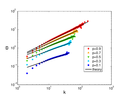
Figure 2: (Color online) Scaling of $\Theta=\langle{\Theta_{i}}\rangle_{k_{i}=k}$, the average of $\Theta_{i}$, performed over nodes of degree $k_{i}=k$, versus the degree $k$. This scaling allows us to define the exponents $\theta=\theta(p)$ defined by Eq. $(\ref{Theta})$. The figure is obtained by performing $100$ realizations of networks of size $n=100\,000$.

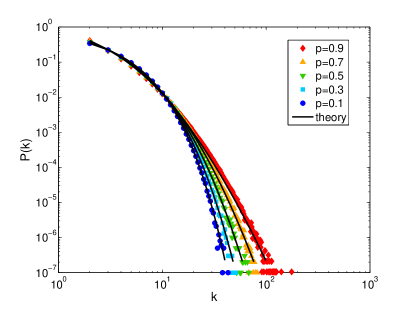
Figure 3: (Color online) Degree distributions of the basic model, for different values of the parameter $p$. The continuous lines indicate the theoretical predictions of Eq. $(\ref{Pk})$, the symbols the distributions obtained from numerical simulations of the model. The figure is obtained by performing $100$ realizations of networks of size $n=100\,000$.

We remark that this model has been already studied in independent papers by Vazquez Vázquez (2003) and Jackson Jackson and Rogers (2007), who claimed that the model yields always power law degree distributions. Our derivation for $m=2$ shows that this is not correct, in general, and in particular it is not correct when the growing network exhibits degree correlations, in which case we do not expect that the probability to reach a node of degree $k_{A}$ by following a link is proportional to $k_{A}$. When the network is correlated we always find $\theta<1$, i.e. the effective link probability is sublinear in the degree of the target node.

We note however, that the duplication model Solé et al. (2002); Krapivsky and Redner (2005); Ispolatov et al. (2005); Lambiotte , in which every new node is attached to a random node and to each of its neighbor with probability $p$, displays at the same time degree correlations and power-law degree distribution.

We also find that the model spontaneously generates communities during the evolution of the system. To quantify how pronounced communities are, we use a measure called embeddedness, which estimates how strongly nodes are attached to their own cluster. Embeddedness, which we shall indicate with $\xi$, is defined as follows:

$$\xi=\frac{1}{n_{c}}\sum_{c}\frac{k_{\mathrm{in}}^{c}}{k_{\mathrm{tot}}^{c}}\,,$$ (12)

where $k_{\mathrm{in}}^{c}$ and $k_{\mathrm{tot}}^{c}$ are the internal and the total degree of community $c$ and the sum runs over all $n_{c}$ communities of the network. If the community structure is strong, most of the neighbors of each node in a cluster will be nodes of that cluster, so $k_{\mathrm{in}}^{c}$ will be close to $k_{\mathrm{tot}}^{c}$ and $\xi$ turns out to be close to $1$; if there is no community structure $\xi$ is close to zero. However, one could still get values of embeddedness which are not too small, even in random graphs, which have no modular structure, as $k_{\mathrm{in}}^{c}$ might still be sizeable there. To eliminate such borderline cases, we introduce a new variable, the node-based embeddedness, that we shall indicate with $\xi_{n}$. It is based on the idea that for a node to be properly assigned to a cluster, it must have more neighbors in that cluster than in any of the others. This leads to the following definition

$$\xi_{n}=\frac{1}{n}\sum_{i}\frac{k_{i,\mathrm{in}}-k_{i,\mathrm{ext}}^{\mathrm{max}}}{k_{i}}\,,$$ (13)

where $k_{i,\mathrm{in}}$ is the number of neighbors of node $i$ in its cluster, $k_{i,\mathrm{ext}}^{\mathrm{max}}$ is the maximum number of neighbors of $i$ in any one other cluster and $k_{i}$ the total degree of $i$. The sum runs over all $n$ nodes of the graph. For a proper community assignment, the difference $k_{i,\mathrm{in}}-k_{i,\mathrm{ext}}^{\mathrm{max}}$ is expected to be positive, negative if the node is misclassified. In a random graph, and for subgraphs of approximately the same size, $\xi_{n}$ would be around zero. In a set of disconnected cliques (a clique being a subgraph where all nodes are connected to each other), which is the paradigm of perfect community structure, $\xi_{n}$ would be $1$.

In Fig. 4a we show a heat map for $\xi_{n}$ as a function of the two main variables of the model, the probability $p$ and the number of edges per node $m$, which is half the average degree. Communities were detected with non-hierarchical Infomap Rosvall and Bergstrom (2008) in all cases. Results obtained by applying the Louvain algorithm Blondel et al. (2008) (taking the most granular level to avoid artifacts caused by the resolution limit Fortunato and Barthélemy (2007)) yield a consistent picture. All networks are grown until $n=50\,000$ nodes.

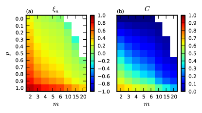
Figure 4: (Color online) Heat map of node-based embeddedness (a) and average clustering coefficient (b) as a function of $p$ and $m$ for the basic model. Community structure (higher embeddedness and clustering coefficient) is pronounced in the lower left region when $m$ is not too large (sparse graphs) and when the probability of triadic closure $p$ is very high. For each pair of parameter values we report the average over $50$ network realizations. The white area in the upper right corresponds to systems where a single community, consisting of the whole network, is found. Here one would get a maximum value $1$ for $\xi_{n}$, but it is not meaningful, hence we discard this portion of the phase diagram, as well as in Figs. 7 and 8.

We see that large values of $\xi_{n}$ are associated to the bottom left portion of the diagram, corresponding to high values of the probability of triadic closure and to low values of degree. So, a high density of triangles ensures the formation of clusters, provided the network is sufficiently sparse. In Fig. 4b we present an analogous heat map for the average clustering coefficient $C$, which is defined Watts and Strogatz (1998) as

$$C=\frac{1}{n}\sum_{i}\sum_{j,k}\frac{a_{ij}a_{jk}a_{ki}}{k_{i}(k_{i}-1)}$$ (14)

where $a_{ij}$ is the element of the adjacency matrix of the graph and $k_{i}$ is again the degree of node $i$. Fig. 4b confirms that $C$ is the largest when $p$ is high and $m$ is low, as expected.

The mechanism of formation and evolution of communities is schematically illustrated in Fig. 5. When the first denser clumps of the network are formed (a), out of random fluctuations in the density of triangles newly added nodes are more likely to close triads within the protoclusters than between them (b).

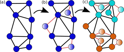
Figure 5: (Color online) Schematic illustration of the formation and evolution of communities. Initial inhomogeneities in the link density make more likely the closure of triads in the denser parts, that keep growing until they become themselves inhomogeous, leading to a split into smaller communities (different colors).

As more nodes and links are added, the protoclusters become larger and larger and their internal density of links becomes inhomogenous, so there will be a selective triadic closure within the denser parts, which yields a separation into smaller clusters (c). This cycle of growing and splitting plays repeatedly along the evolution of the system.

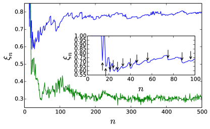
Figure 6: (Color online) Evolution of node-based community embeddedness $\xi_{n}$ along the growth of the network. The curves refer to the extreme cases of absence of triadic closure (lower curve), yielding a random graph without communities, and of systematic triadic closure (upper curve), yielding a graph with pronounced community structure. For the latter case, we magnify in the inset the initial portion of the curve, to highlight the sudden drops of $\xi_{n}$, indicated by the arrows, which correspond to the breakout of clusters into smaller ones.

In Fig. 6 we show the time evolution of the node-based embeddedness $\xi_{n}$ during the growth of the system, until $500$ nodes are added to the network, $m=2$. We consider the two extreme situations $p=0$, corresponding to the absence of triadic closure and $p=1$, where both links close a triangle every time and there is no additional noise. In the first case (green line), after a transient, $\xi_{n}$ sets to a low value, with small fluctuations; in the case with pure triadic closure, instead, the equilibrium value is much higher, indicating strong community structure, and fluctuations are modest. In contrast with the random case, we recognize a characteristic pattern, with $\xi_{n}$ increasing steadily and then suddenly dropping. The smooth increase of $\xi_{n}$ signal that the communities are growing, the rapid drop that a cluster splits into smaller pieces: in the inset such breakouts are indicated by arrows. Embeddedness drops when clusters break up because the internal degrees $k_{i,\mathrm{in}}$ of the nodes of the fragments in Eq. 13 suddenly decrease, since some of the old internal neighbors belong to a different community, while the values of $k_{i,\mathrm{ext}}^{\mathrm{max}}$ are typically unaffected.

III Preferential attachment or temporal network models including triadic closure

The scenario depicted in Section II is not limited to the basic model we have investigated, but it is quite general. To show this, we consider here two other models based on triadic closure.

The model by Holme and Kim Holme and Kim (2002) is a variant of the Barabási-Albert model of preferential attachment (BA model) which generate scale-free networks with clustering. The new node joining the network sets a link with an existing node, chosen with a probability proportional to the degree of the latter, just like in the BA model. The other $m-1$ links coming with the new node, however, are attached with a probability $P_{t}$ to a random neighbor of the node which received the most recent preferentially-attached link, closing a triangle, and with a probability $1-P_{t}$ to another node chosen with preferential attachment. By varying $P_{t}$ it is possible to tune the level of clustering into the network, while the degree distribution is the same as in the BA model, i.e. a power law with exponent $-3$, for any value of $P_{t}$.

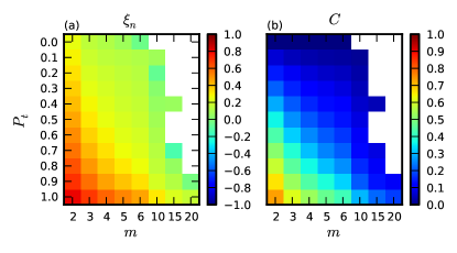
Figure 7: (Color online) Heat map of node-based embeddedness (a) and average clustering coefficient (b) as a function of $P_{t}$ and $m$ for the model by Holme and Kim Holme and Kim (2002). For each pair of parameter values we report the average over $50$ network realizations. The white area in the upper right corresponds to systems where a single community, consisting of the whole network, is found, which is not interesting. The diagrams look qualitatively similar to that of the basic model (Fig. 4), with highest embeddedness and clustering coefficient in the lower left region.

In Fig. 7 we show the same heat map as in Fig. 4 for this model, where we now report the probability $P_{t}$ on the y-axis. Networks are again grown until $n=50\,000$ nodes. The picture is very similar to what we observe for the basic model.

The model by Marsili et al. Marsili et al. (2004), at variance with most models of network formation, is not based on a growth process. The model is a model for temporal networks Holme and Saramäki (2012), in which the links are created and destroyed on the fast time scale while the number of nodes remains constant. The starting point is a random graph with $n$ nodes. Then, three processes take place, at different rates:

1. any existing link vanishes (rate $\lambda$);

2. a new link is created between a pair of nodes, chosen at random (rate $\eta$);

3. a triangle is formed by joining a node with a random neighbor of one of his neighbors, chosen at random (rate $\xi_{M}$).

In our simulations we start from a random network of $n=50\,000$ nodes with average degree $10$. The three rates $\lambda$, $\eta$ and $\xi_{M}$ can be reduced to two independent parameters, since what counts is their relative size. The number of links deleted at each iteration is proportional to $\lambda M$, where $M$ is the number of links of the network, while the number of links created via the two other processes is proportional to $\eta n$ and $\xi_{M}n$, respectively. The number of links $M$ varies in time but in order to get a non-trivial stationary state, one should reach an equilibrium situation where the numbers of deleted and created links match. A variety of scenarios are possible, depending on the choices of the parameters. For instance, if $\xi_{M}$ is set equal to zero, there are no triads, and what one gets at stationarity is a random graph with average degree $2\eta/\lambda$. So, if $\eta\ll\lambda$, the graph is fragmented into many small connected components. In one introduces triadic closure, the clustering coefficient grows with $\xi_{M}$ if the network is fragmented, as triangles concentrate in the connected components. Moreover the model can display a veritable first order phase transition and in a region of the phase diagram displays two stable phases: one corresponding to a connected network with large average clustering coefficient and the other one corresponding to a disconnected network. Interestingly, if there is a dense single component, the clustering coefficient decreases with $\xi_{M}$. The degree distribution can follow different patterns too: it is Poissonian in the diluted phase, where the system is fragmented, and broad in the dense phase, where the system consists of a single component with an appreciable density of links. In Fig. 8 we show the analogous heat map as in Figs. 4 and 7, for the two parameters $\lambda$ and $\xi_{M}$. The third parameter $\eta=1$. We consider only configurations where the giant component covers more than a half of the nodes of the network. The diagrams are now different because of the different role of the parameters, but the picture is consistent nevertheless. The clustering coefficient $C$ is highest when the ratio of $\lambda$ and $\xi_{M}$ lies within a narrow range, yielding a sparse network with a giant component having a high density of triangles and a corresponding presence of strong communities.

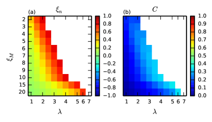
Figure 8: (Color online) Heat map of node-based embeddedness (a) and average clustering coefficient (b) as a function of the rates $\lambda$ and $\xi_{M}$ for the model by Marsili et al. Marsili et al. (2004) ($\eta=1$). For each pair of parameter values we report the average over $50$ network realizations. The white area in the upper right corresponds to systems where a single community, consisting of the whole network, is found, which is not interesting. These diagrams have better communities (higher embeddedness and clustering coefficient) towards the upper right, different from those in Figs. 4 and 7, because of the different meaning and effect of the parameters. However, there is a strong correspondence between high clustering coefficient and strong community structure, as in the other models.

IV The basic model including triadic closure and fitness of the nodes

In this Section we introduce a variant of the basic model, where the link attractivity depends on some intrinsic fitness of the nodes. We will assume that the nodes are not all equal and assign to each node $i$ a fitness $\eta_{i}$ representing the ability of a node to attract new links. We have chosen to parametrize the fitness with a parameter $\beta>0$ by setting

$$\eta_{i}=e^{-\beta\epsilon_{i}}\,,$$ (15)

with $\epsilon$ chosen from a distribution $g(\epsilon)$ and $\beta$ representing a tuning parameter of the model. We take

$$g(\epsilon)=(1+\nu)\epsilon^{\nu}\,,$$ (16)

with $\epsilon\in(0,1)$. When $\beta=0$ all the fitness values are the same, when $\beta$ is large small differences in the $\epsilon_{i}$ cause large differences in fitness. For simplicity we assume that the fitness values are quenched variables assigned once for all to the nodes. As in the basic model without fitness, the starting point is a small connected network of $n_{0}$ nodes and $m_{0}\geq m$ links. The model contains two ingredients:

• Growth. At time $t$ a new node is added to the network with $m\geq 2$ links.

• Proximity and fitness bias. The probability to attach the new node to node $i_{1}$ depends on the order in which links are added.
  The first link of the new node is attached to a random node $i_{1}$ of the network with probability proportional to its fitness. The probability that the new node is attached to node $i_{1}$ is then given by

  $$\Pi^{[0]}({i_{1}})=\frac{\eta_{i_{1}}}{\sum_{j}\eta_{j}}\,.$$ (17)

  For $m=2$ the second link is attached to a node of the network chosen according to its fitness, as above, with probability $1-p$, while with probability $p$ it is attached to a node chosen randomly between the neighbors of the node $i_{1}$ with probability proportional to its fitness. Therefore in the first case the probability to attach to a node $i_{2}\neq i_{1}$ is given by

  $$\Pi^{[0]}(i_{2})=\frac{\eta_{i_{2}}(1-\delta_{i_{1},i_{2}})}{\sum_{j\neq i_{1}}\eta_{j}}\,,$$ (18)

  with $\delta_{i_{1},i_{2}}$ indicating the Kronecker delta, while in the second case the probability $\Pi^{[1]}({i_{2}})$ that the new node links to node $i_{2}$ is given by

  $$\Pi^{[1]}(i_{2})=\frac{\eta_{i_{2}}a_{i_{1},i_{2}}}{\sum_{j}\eta_{j}a_{i_{1},j}}\,,$$ (19)

  where $a_{ij}$ indicates the matrix element $(i,j)$ of the adjacency matrix of the network.

• Further edges. For $m>2$, further edges are added according to the “second link” rule in the previous point. With probability $p$ an edge is added to a neighbor of the first node $i_{1}$, not already attached to the new node, according to the fitness rule. With probability $1-p$, a link is set to any node in the network, not already attached to the new node, according to the fitness rule.

For simplicity we shall consider here the case $m=2$. The probability that a node $i$ acquires a new link at time $t$ is given by

$$\frac{e^{-\beta\epsilon_{i}}}{t}\left[(2-p)+p\sum_{j}\frac{a_{ij}}{\sum_{r}\eta_{r}a_{jr}}\right]\,.$$ (20)

Similarly to the case without fitness, here we will assume, supported by simulations, that

$$\Theta_{i}=p\sum_{j}\frac{\eta_{j}a_{ij}}{\sum_{r}\eta_{r}a_{jr}}\simeq ck_{i}^{\theta(\epsilon)}\,,$$ (21)

where, for every value of $p$, $\theta=\theta(\epsilon)\leq 1$ and $c=c(\epsilon)$.

We can write the master equation for the average number $n_{k,\epsilon}(t)$ of nodes of degree $k$ and energy $\epsilon$ at time $t$, as

$$n_{k,\epsilon}(t+1) = n_{k,\epsilon}(t)$$ (22)

$$+\frac{e^{-\beta\epsilon}[2-p+c(\epsilon)(k-1)^{\theta}]}{t}n_{k-1,\epsilon}(t)(1-\delta_{k,2})$$

$$-\frac{e^{-\beta\epsilon}[2-p+c(\epsilon)k^{\theta(\epsilon)}]}{t}n_{k,\epsilon}(t)+\delta_{k,2}g(\epsilon)\,.$$

In the limit of large values of $t$ we assume that $n_{k,\epsilon}/t\to P^{\epsilon}(k)$, and therefore we find that the solution for $P^{\epsilon}(k)$ is given by

$$P^{\epsilon}(k) = C(\epsilon)\frac{1}{1+e^{-\beta\epsilon}[2-p+c(\epsilon)k^{\theta(\epsilon)}]}$$ (23)

$$\times\prod_{j=1}^{k-1}\left\{1-\frac{1}{1+e^{-\beta\epsilon}[2-p+c(\epsilon)j^{\theta(\epsilon)}]}\right\}\,,$$

where $C(\epsilon)$ is the normalization factor. This expression for $\theta(\epsilon)<1$ can be approximated in the continuous limit by

$$P^{\epsilon}(k) \simeq D(\epsilon)\frac{e^{-(k-1)G[k-1,\epsilon,\theta(\epsilon),c(\epsilon)]}}{1+e^{-\beta\epsilon}[2-p+c(\epsilon)k^{\theta(\epsilon)}]},$$ (24)

where $D(\epsilon)$ is the normalization constant and $G(k,\epsilon,\theta,c)$ is given by

$$G(k,\epsilon,\theta,c) = -\theta_{2}F_{1}\left(1,\frac{1}{\theta},1+\frac{1}{\theta},-\frac{ck^{\theta}}{2-p+e^{\beta\epsilon}}\right)$$ (25)

$$+\theta_{2}F_{1}\left(1,\frac{1}{\theta},1+\frac{1}{\theta},-\frac{ck^{\theta}}{2-p}\right)$$

$$+\log\left(1-\frac{1}{1+\frac{e^{\beta\epsilon}}{2-p+ck^{\theta}}}\right)\,.$$

When $\theta(\epsilon)=1$, instead, we can approximate $P^{\epsilon}(k)$ with a power law, i.e.

$$P^{\epsilon}(k)\simeq D(\epsilon)\left[1+e^{-\beta\epsilon}\left(2-p+c(\epsilon)k\right)\right]^{-\frac{e^{-\beta\epsilon}}{c(\epsilon)}-1}.$$ (26)

Therefore, the degree distribution $P(k)$ of the entire network is a convolution of the degree distributions $P^{\epsilon}(k)$ conditioned on the value of $\epsilon$, i.e.

$$P(k)=\int d\epsilon P^{\epsilon}(k)\,.$$ (27)

As a result of this expression, we found that the degree distribution can be a power law also if the network exhibits degree correlations and $\theta(\epsilon)<1$ for every value of $\epsilon$. Moreover we observe that for large values of the parameter $\beta$ the distribution becomes broader and broader until a condensation transition occurs at $\beta=\beta_{c}$ with the value of $\beta_{c}$ depending on both the parameters $\nu$ and $p$ of the model. For $\beta>\beta_{c}$ successive nodes with maximum fitness (minimum value of $\epsilon$) become “superhubs”, attracting a finite fraction of all the links, similarly to what happens in Ref. Bianconi and Barabási (2001). In Fig. 9 we see the degree distribution of model, obtained via numerical simulations, for different values of $\beta$. The continuous lines, illustrating the theoretical behavior, are well aligned with the numerical results, as long as $\beta<\beta_{c}$.

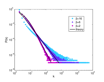
Figure 9: (Color online) Degree distribution of the model with fitness, for three values of the parameter $\beta$, which indicates the heterogeneity of the distribution of the fitness of the nodes. Symbols stand for the results obtained by building the network via simulations, continuous lines for our analytical derivations. The figure is obtained by performing $100$ realizations of networks of size $n=100\,000$ with $\nu=6$.

In Fig. 10 we show the heat map of $\xi_{n}$ and $C$ for the model, as a function of the parameters $p$ and $\beta$. The number of edges per node is $m=2$, and the networks consist of $50\,000$ nodes. Everywhere in this work, we set the parameter $\nu=6$. For $\beta=0$ all nodes have identical fitness and the model reduces itself to the basic model. So we recover the previous results, with the emergence of communities for sufficiently large values of the probability of triadic closure $p$, following a large density of triangles in the system. The situation changes dramatically when $\beta$ starts to increase, as we witness a progressive weakening of community structure, while the clustering coefficient keeps growing, which appears counterintuitive. In the analogous diagrams for $m=5$, we see that this pattern holds, though with a weaker overall community structure and lower values of the clustering coefficient.

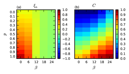
Figure 10: (Color online) Heat map of node-based embeddedness (a) and average clustering coefficient (b) as a function of the probability of triadic closure $p$ and the heterogeneity parameter $\beta$ of the fitness distribution of the nodes, for the model with fitness. The number of new edges per node is $m=2$. For each pair of parameter values we report the average over $50$ network realizations. When $\beta=0$ we recover the basic model, without fitness. We see the highest values of embeddedness in the lower left, while highest values of the clustering coefficient are in the lower right. When $\beta$ increases, we see a drastic change of structure in contrast to the previous pattern: communities disappear, whereas the clustering coefficient gets higher.

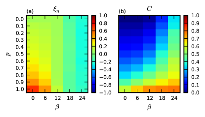
Figure 11: (Color online) Same as Fig. 10, but for $m=5$. The picture is consistent with the case $m=2$, but communities are less pronounced.

When $\beta$ is sufficiently large, communities disappear, despite the high density of triangles. To check what happens, we compute the probability distribution of the scaled link density $\tilde{\rho}$ and the node-based embeddedness $\xi_{n}$ of the communities of the networks obtained from $100$ runs of the model, for three different values of $\beta$: $0$, $6$ and $20$. All networks are grown until $100\,000$ nodes. The scaled link density $\tilde{\rho}$ of a cluster is defined Lancichinetti et al. (2010) as

$$\tilde{\rho}=\frac{2l_{c}}{n_{c}-1}\,,$$ (28)

where $l_{c}$ and $n_{c}$ are the number of internal links and of nodes of cluster $c$. If the cluster is tree-like, $\tilde{\rho}\approx 2$, if it is clique-like it $\tilde{\rho}\approx n_{c}$, so it grows linearly with the size of the cluster. The distributions of $\xi_{n}$ and $\tilde{\rho}$ are shown in Fig. 12.

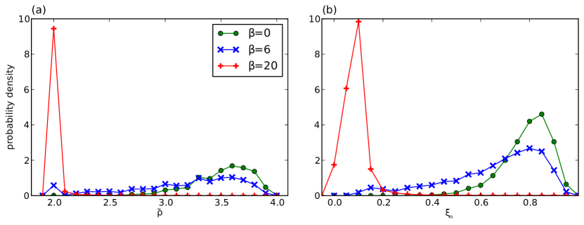
Figure 12: (Color online) Probability distributions of the scaled link density $\tilde{\rho}$ (left) and node-based embeddedness $\xi_{n}$ (right) of the communities of the fitness model, for $m=2$ and $\beta=0,6,20$. For each $\beta$-value we derived $100$ network realizations, each with $100\,000$ nodes. We see that at $\beta=0$, the detected communities satisfy the expectations of good communities, while at $\beta=20$ they do not.

They are peaked, but the peaks undergo a rapid shift when $\beta$ goes from $0$ to $20$. The situation resembles what one usually observes in first-order phase transitions. The embeddedness ends up peaking at low values, quite distant from the maximum $1$, while the scaled link density eventually peaks sharply at $2$, indicating that the subgraphs are effectively tree-like.

What kind of objects are we looking at? To answer this question, in Figs. 13 and 14 we display two pictures of networks obtained by the fitness model, for $\beta=0$ and $\beta=20$, respectively. The number of nodes is $2\,000$, and the number of edges per node $m=2$. The probability of triadic closure is $p=0.97$, as we want a very favorable scenario for the emergence of structure.

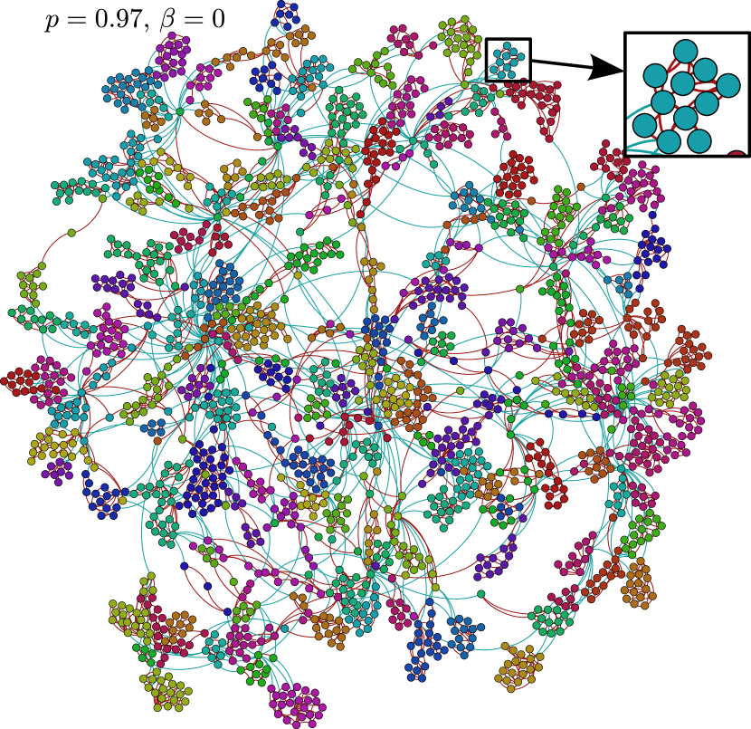
Figure 13: (Color online) Picture of a network with $2\,000$ nodes generated by the fitness model, for $p=0.97$, $m=2$ and $\beta=0$. Since $\beta=0$ fitness does not play a role and we recover the results of the basic model. Colors indicate communities as detected by the non-hierarchical Infomap algorithm Rosvall and Bergstrom (2008).

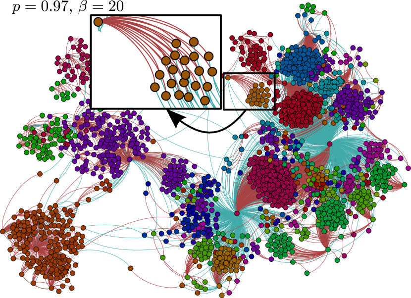
Figure 14: (Color online) Picture of a network with $2\,000$ nodes generated by the fitness model, for $p=0.97$, $m=2$ and $\beta=20$. The growing process is the same as in Fig. 13, but the addition of fitness changes the structural organization of the network. As seen in the inset, node aggregations form around hub nodes with high fitness. Looking at the inset we see that such aggregations do not satisfy the typical requirements for communities: they are internally tree-like, and there are more external edges (blue or light gray) than internal (red or dark gray) touching its nodes. In particular, internal edges only go from regular nodes to superhubs.

The subgraphs found by our community detection method (non-hierarchical Infomap, but the Louvain method yields a similar picture) are identified by the different colors. The insets show an enlarged picture of the subgraphs, which clarify the apparent puzzle delivered by the previous diagrams. For the basic model $\beta=0$ (Fig. 13), the subgraphs are indeed communities, as they are cohesive objects which are only loosely connected to the rest of the graph. The situation remains similar for low values of $\beta$. However, for sufficiently high $\beta$ (Fig. 14), a phenomenon of link condensation takes place, with a few superhubs attracting most of the links of the network Bianconi and Barabási (2001). Most of the other nodes are organized in groups which are “shared” between pairs (for $m=2$, more generally $m$-ples) of superhubs (see figure). The community embeddedness is low because there are always many links flowing out of the subgraphs, towards superhubs. Besides, since the superhubs are all linked to each other, this generates high clustering coefficient for the subgraphs, as observed in Figs. 10 and 11. In fact, the clustering coefficient for the non-hubs attains the maximum possible value of $1$, as their neighbors are nodes which are all linked to each other.

V Conclusions

Triadic closure is a fundamental mechanism of link formation, especially in social networks. We have shown that such mechanism alone is capable to generate systems with all the characteristic properties of complex networks, from fat-tailed degree distributions to high clustering coefficients and strong community structure. In particular, we have seen that communities emerge naturally via triadic closure, which tend to generate cohesive subgraphs around portions of the system that happen to have higher density of links, due to stochastic fluctuations. When clusters become sufficiently large, their internal structure exhibits in turn link density inhomogeneities, leading to a progressive differentiation and eventual separation into smaller clusters (separation in the sense that the density of links between the parts is appreciably lower than within them). This occurs both in the basic version of network growth model based on triadic closure, and in more complex variants. The strength of community structure is the higher, the sparser the network and the higher the probability of triadic closure.

We have also introduced a new variant, in that link attractivity depends on some intrinsic appeal of the nodes, or fitness. Here we have seen that, when the distribution of fitness is not too heterogeneous, community structure still emerges, though it is weaker than in the absence of fitness. By increasing the heterogeneity of the fitness distribution, instead, we observe a major change in the structural organization of the network: communities disappear and are replaced by special subgraphs, whose nodes are connected only to superhubs of the network, i.e. nodes attracting most of the links. Such structural phase transition is associated to very high values of the clustering coefficient.