A Posteriori Error Estimation of $hp$-$\operatorname*{dG}$ Finite Element Methods for Highly Indefinite Helmholtz Problems (extended version)

Abstract

In this paper, we will consider an $hp$-finite elements discretization of a highly indefinite Helmholtz problem by some $\operatorname{dG}$ formulation which is based on the ultra-weak variational formulation by Cessenat and Deprés.

We will introduce an a posteriori error estimator and derive reliability and efficiency estimates which are explicit with respect to the wavenumber and the discretization parameters $h$ and $p$. In contrast to the conventional conforming finite element method for indefinite problems, the $\operatorname{dG}$ formulation is unconditionally stable and the adaptive discretization process may start from a very coarse initial mesh.

Numerical experiments will illustrate the efficiency and robustness of the method.

AMS Subject Classifications: 35J05, 65N12, 65N30

Key words: Helmholtz equation at high wavenumber, $hp$-finite elements, a posteriori error estimation, discontinuous Galerkin methods, ultra-weak variational formulation

1 Introduction

High frequency scattering problems are ubiquitous in many fields of science and engineering and their reliable and efficient numerical simulation pervades numerous engineering applications such as detection (e.g., radar), communication (e.g., wireless), and medicine (e.g., sonic imaging) ([32], [1]). These phenomena are governed by systems of linear partial differential equations (PDEs); the wave equation for elastic waves and the Maxwell equations for electromagnetic scattering. We are here interested in time-harmonic problems where the equation can be reduced to purely spatial problems; for high frequencies these PDEs become highly indefinite and the development of accurate numerical solution methods is far from being in a mature state.

In this paper we will consider the Helmholtz problem with high wavenumber as our model problem. Although the continuous problem with appropriate boundary conditions has a unique solution, conventional $hp$-finite element methods require a minimal resolution condition such that existence and uniqueness is guaranteed on the discrete level (see, e.g., [30], [29], [37], [38], [11]). However, this condition, typically, contains a generic constant $C$ which is either unknown for specific problems or only very pessimistic estimates are available. This is one of the major motivations for the development of stabilized formulations such that the discrete system is always solvable – well-known examples include least square techniques [40, 23, 24, 22] and discontinuous Galerkin ($\operatorname{dG}$) methods [18, 19, 20, 46, 48]. These formulations lead to discrete systems which are unconditionally stable, i.e., no resolution condition is required. Although convergence starts for these methods only after a resolution condition is reached, the stability of the discrete system is considerably improved. The Ultra Weak Variational Formulation (UWVF) of Cessenat and Després [9, 10, 13] can be understood as a $\operatorname*{dG}$-method that permits the use of non-standard, discontinuous local discretization spaces such as plane waves (see [21, 28, 25, 8]). In this paper we will employ a $hp$-$\operatorname*{dG}$-finite element method based on the UWVF which was developed in [21] and generalized in [36].

Our focus here is on the development of an a posteriori error estimator for this formulation and its analysis which is explicit with respect to the discretization parameters $h$, $p$, and the wavenumber. In contrast to definite elliptic problems, there exist only relatively few publications in the literature on a posteriori estimation for highly indefinite problems (cf. [31], [3], [4], [43], [16]). The papers which are closely related to our work are [26] and [16]: a) In [26], an a posteriori error estimator for the Helmholtz problem has been developed for the interior penalty discontinuous Galerkin (IPDG) method and reliability, efficiency, and convergence of the resulting adaptive method is proved. In contrast, we do not prove the convergence of the resulting adaptive method for our $\operatorname{dG}$-formulation. On the other hand, our estimators are properly weighted with the polynomial degree and the estimates are explicit with respect to the wavenumber $k$, the mesh width $h$, and the polynomial degree $p$. In addition, the dependence of the constants in the estimates on the wavenumber $k$ are milder in our approach compared to [26]; b) In [16], a residual a posteriori error estimator (cf. [5], [6], [2], [45]) has been developed for the conventional $hp$-finite element method. Although efficiency and reliability estimates have been proved, a strict minimal resolution condition is required for the initial finite element space and this is a severe drawback in the context of adaptive discretization.

We will prove in this paper, that our a posteriori error estimator for the $hp$-$\operatorname*{dG}$-finite element method does not require this strict condition and allows to start the adaptive discretization process from very coarse finite element meshes and no a priori information is required.

The paper is organized as follows. In Section 2, we will introduce the model problem and its $\operatorname{dG}$-discretization by $hp$-finite elements. We will recall its unconditional stability and state the quasi-optimal convergence.

Section 3 is devoted to the definition of the residual a posteriori error estimator and we will prove its reliability and efficiency.

In Section 4 we will present an adaptive discretization process and report on numerical experiments which illustrate the behavior of the method for specific model problems such as smooth problems, problems with singularities, problems with constant, varying, and discontinuous wavenumber, and the dependence on the polynomial degree of approximation.

The proof of reliability employs a new $hp$-$C^{1}$ Clément-type interpolation operator which will be defined in Appendix A and $hp$-explicit approximation results are proved.

2 Discontinuous Galerkin (dG)-Discretization

2.1 Helmholtz Equation with Robin Boundary Conditions

Let $\Omega\subset\mathbb{R}^{2}$ be a bounded Lipschitz domain with boundary $\partial\Omega$. The scalar product in $L^{2}\left(\Omega\right)$ is denoted by $\left(u,v\right):=\int_{\Omega}u\overline{v}$ and the norm by $\left\|\cdot\right\|$.

For $s>0$, the space $H^{s}\left(\Omega\right)$ is the usual Sobolev space with norm $\left\|\cdot\right\|_{H^{s}\left(\Omega\right)}$. The dual space is denoted by $\left(H^{s}\left(\Omega\right)\right)^{\prime}$ and the trace spaces by $H^{\sigma}\left(\partial\Omega\right)$ with norm $\left\|\cdot\right\|_{H^{\sigma}\left(\partial\Omega\right)}$. For $\sigma=0$, we write $\left\|\cdot\right\|_{\partial\Omega}$ short for $\left\|\cdot\right\|_{L^{2}\left(\partial\Omega\right)}$. The seminorms containing only the highest derivatives are denoted by $\left|\cdot\right|_{H^{s}\left(\Omega\right)}$ and $\left|\cdot\right|_{H^{\sigma}\left(\partial\Omega\right)}$.

For given $f\in L^{2}(\Omega)$, $g\in L^{2}(\partial\Omega)$ we consider the Helmholtz equation with Robin boundary condition

$$-\Delta u-k^{2}u =f \text{in~{}}\Omega,$$

$$\partial_{\mathbf{n}}u+iku =g \text{on~{}}\partial\Omega,$$

where $\partial_{\mathbf{n}}u$ denotes the outer normal derivative of $u$ on the boundary. In most parts of this paper we assume that $k$ is a positive constant. This is a simplification compared to the following more general case: There exist positive constants $\kappa$ and $k_{\max}$ such that

$$\begin{array}[c]{cll}k\in L^{\infty}\left(\Omega,\mathbb{R}\right),&&1<\kappa\leq k\left(x\right)\leq k_{\max}<\infty,\\[3.0pt] k=\kappa&&\text{in a neighborhood of }\partial\Omega.\end{array}$$ (2.1)

We define the method for, possibly, variable wavenumbers $k$ which satisfy (2.1) while the error analysis is restricted to the constant case. In the section on numerical experiments, we will again consider variable wavenumbers $k$.

The weak formulation reads: Find $u\in H^{1}\left(\Omega\right)$ such that

$$a\left(u,v\right)=F\left(v\right)\qquad\forall v\in H^{1}\left(\Omega\right)$$ (2.2a)

with the sesquilinear form $a:H^{1}\left(\Omega\right)\times H^{1}\left(\Omega\right)\rightarrow\mathbb{C}$ and linear form $F:H^{1}\left(\Omega\right)\rightarrow\mathbb{C}$ defined by

$$a\left(u,v\right):=\int_{\Omega}\left(\left\langle\nabla u,\overline{\nabla v}\right\rangle-k^{2}u\overline{v}\right)+\operatorname*{i}\int_{\partial\Omega}ku\overline{v}\quad\text{and\quad}F\left(v\right):=\int_{\Omega}f\overline{v}+\int_{\partial\Omega}g\overline{v}.$$ (2.2b)

The assumptions on the data can be weakened to $f\in(H^{1}(\Omega))^{\prime}$ and $g\in H^{-1/2}(\partial\Omega)$. In this case the integrals in (2.2b) are understood as dual pairings.

It is well-known that this problem has a unique solution which depends continuously on the data.

Definition 2.1.

Let $k$ satisfy (2.1). On $H^{1}\left(\Omega\right)$, we introduce the norm

$$\left\|u\right\|_{\mathcal{H}}:=\left\|\nabla u\right\|+\left\|ku\right\|.$$

Theorem 2.2.

Let $\Omega\subseteq\mathbb{R}^{2}$ be a bounded Lipschitz domain and let $k=\kappa>1$ be constant.

1. There exists a constant $C\left(\Omega,\kappa\right)>0$ such that for every $f\in\left(H^{1}\left(\Omega\right)\right)^{\prime}$ and $g\in H^{-1/2}\left(\partial\Omega\right)$, there exists a unique solution $u\in H^{1}\left(\Omega\right)$ of problem (2.2) which satisfies

   $$\left\|u\right\|_{\mathcal{H}}\leq C\left(\Omega,\kappa\right)\left(\left\|F\right\|_{\left(H^{1}\left(\Omega\right)\right)^{\prime}}+\left\|g\right\|_{H^{-1/2}\left(\partial\Omega\right)}\right).$$

2. Let $\Omega\subseteq\mathbb{R}^{2}$ be a bounded star-shaped domain with smooth boundary or a bounded convex domain. There exists a constant $C\left(\Omega\right)>0$ (depending only on $\Omega$) such that for any $f\in L^{2}\left(\Omega\right)$, $g\in H^{1/2}\left(\partial\Omega\right)$, the solution of (2.2) satisfies

   $$\left\|u\right\|_{\mathcal{H}} \leq C\left(\Omega\right)\left(\left\|f\right\|+\left\|g\right\|_{\partial\Omega}\right),$$

   $$\left|u\right|_{H^{2}\left(\Omega\right)} \leq C\left(\Omega\right)\left(1+\kappa\right)\left(\left\|f\right\|+\left\|g\right\|_{\partial\Omega}+\left\|g\right\|_{H^{1/2}\left(\partial\Omega\right)}\right).$$

For a proof we refer to [34, Prop. 8.1.3 and .4].

Remark 2.3.

Let $\Omega\subseteq\mathbb{R}^{2}$ be a polygonal Lipschitz domain and let $k=\kappa>1$ be a constant. For $f\in L^{2}\left(\Omega\right)$ and $g\in H_{\operatorname*{pw}}^{1/2}\left(\partial\Omega\right):=\left\{g\in L^{2}\left(\partial\Omega\right):g\text{ is edgewise in }H^{1/2}\right\}$, the classical elliptic regularity theory shows that the unique solution $u$ of (2.2) is in $H^{3/2+\varepsilon}(\Omega)$ for some $\varepsilon>0$ depending on $\Omega$ and we briefly sketch the argument: We write (2.2) in the following strong form

$$-\Delta u =\tilde{f}:=f+k^{2}u \text{in }\Omega,$$

$$\partial_{\mathbf{n}}u =\tilde{g}:=g-\operatorname*{i}ku \text{on }\partial\Omega.$$

Since the solution $u$ of (2.2) is in $H^{1}\left(\Omega\right)$, we have $\tilde{f}\in L^{2}\left(\Omega\right)$ and $\tilde{g}\in H_{\operatorname*{pw}}^{1/2}\left(\partial\Omega\right)$. From [38, Lemma A1], we conclude that there exists a lifting operator $\mathcal{L}:H_{\operatorname*{pw}}^{1/2}\left(\partial\Omega\right)\rightarrow H^{2}\left(\Omega\right)$ such that $G:=\mathcal{L}\left(g\right)$ satisfies $\partial_{\mathbf{n}}G=g$ and $\left\|G\right\|_{H^{2}\left(\Omega\right)}\leq C\left\|g\right\|_{H_{\operatorname*{pw}}^{1/2}\left(\partial\Omega\right)}$. Thus, the ansatz $u=u_{0}+\tilde{G}$ with $\tilde{G}:=\mathcal{L}\left(\tilde{g}\right)$ leads to

$$-\Delta u_{0} =\check{f}:=\tilde{f}+\Delta\tilde{G} \text{in }\Omega,$$

$$\partial_{\mathbf{n}}u_{0} =0 \text{on }\partial\Omega$$

with $\check{f}\in L^{2}\left(\Omega\right)$. From [33, (7.22)] we obtain that the solution $u_{0}$, and thus also $u$, then is in $H^{3/2+\varepsilon}\left(\Omega\right)$ for some $\varepsilon>0$.

2.2 hp-Finite Elements

Let $\Omega\subset\mathbb{R}^{2}$ be a polygonal domain and let $\mathcal{T}:=\left\{K_{i}:1\leq i\leq N\right\}$ denote a simplicial finite element mesh which is conforming in the sense that there are no hanging nodes. With each element $K\in\mathcal{T}$ we associate a polynomial degree $p_{K}\in\mathbb{N}_{\geq 1}$.

The diameter of an element $K\in\mathcal{T}$ is denoted by $h_{K}:=\operatorname{diam}K$ and the maximal mesh width is $h_{\mathcal{T}}:=\max\left\{h_{K}:K\in\mathcal{T}\right\}$. The minimal polynomial degree is

$$p_{\mathcal{T}}:=\min\left\{p_{K}:K\in\mathcal{T}\right\}.$$

The shape regularity of $\mathcal{T}$ is described by the constant

$$\rho_{\mathcal{T}}:=\max\left\{\frac{h_{K}}{\operatorname{diam}\mathcal{B}_{K}}:K\in\mathcal{T}\right\},$$ (2.3)

where $\mathcal{B}_{K}$ is the maximal inscribed ball in $K$. Since $\mathcal{T}$ contains finitely many simplices, the constant $\rho_{\mathcal{T}}$ is always bounded but becomes large if the simplices are degenerate, e.g., are flat or needle-shaped. The constants in the following estimates depend on the mesh via the constant $\rho_{\mathcal{T}}$; they are bounded for any fixed $\rho_{\mathcal{T}}$ but, possibly, become large for large $\rho_{\mathcal{T}}$.

Concerning the polynomial degree distribution we assume throughout the paper that the polynomial degrees of neighboring elements are comparable:

$$\rho_{\mathcal{T}}^{-1}\left(p_{K}+1\right)\leq p_{K^{\prime}}+1\leq\rho_{\mathcal{T}}\left(p_{K}+1\right)\qquad\forall K,K^{\prime}\in\mathcal{T}\text{ with }K\cap K^{\prime}\neq\emptyset.$$ (2.4)

By convention the triangles $K\in\mathcal{T}$ are closed sets. The boundary of a triangle $K\in\mathcal{T}$ consists of three one-dimensional (relatively closed) edges which are collected in the set $\mathcal{E}\left(K\right)$. The subset $\mathcal{E}^{I}\left(K\right)\subseteq\mathcal{E}\left(K\right)$ of inner edges consists of all edges $e\in\mathcal{E}\left(K\right)$ whose relative interior lie in (the open set) $\Omega$ while $\mathcal{E}^{B}\left(K\right):=\mathcal{E}\left(K\right)\backslash\mathcal{E}^{I}\left(K\right)$ is the set of boundary edges. Further we set

$$\partial^{B}K:=\partial K\cap\partial\Omega\quad\text{and\quad}\partial^{I}K:=\partial K\backslash\partial^{B}K.$$

The conformity of the mesh implies that any $e\in\mathcal{E}^{I}\left(K\right)$ is shared by two and only two triangles in $\mathcal{T}$. The sets of inner/boundary/all edges $\mathcal{E}^{I}$, $\mathcal{E}^{B}$, $\mathcal{E}$, are defined by

$$\mathcal{E}^{I}:=\left\{e\in\mathcal{E}^{I}\left(K\right):K\in\mathcal{T}\right\},\quad\mathcal{E}^{B}:=\left\{e\in\mathcal{E}^{B}\left(K\right):K\in\mathcal{T}\right\},\quad\mathcal{E}:=\mathcal{E}^{I}\cup\mathcal{E}^{B}.$$

The interior skeleton $\mathfrak{S}^{I}$ is given by

$$\mathfrak{S}^{I}:={\displaystyle\bigcup\limits_{K\in\mathcal{T}}}\partial^{I}K.$$

Next we introduce patches associated with an edge $e$ or an element $K$ of the triangulation

$$\omega_{e}:=\bigcup_{\left\{K^{\prime}\in\mathcal{T}:e\cap K^{\prime}\neq\emptyset\right\}}K^{\prime}\quad\text{and}\quad\omega_{K}:=\bigcup_{\left\{K^{\prime}\in\mathcal{T}:K\cap K^{\prime}\neq\emptyset\right\}}K^{\prime}.$$

Furthermore, we employ the notation

$$p_{e}:=\min_{\begin{subarray}{c}K\in\mathcal{T}\\ e\subset\partial K\end{subarray}}p_{K}\quad\text{and\quad}h_{e}:=\left|e\right|\quad\text{with the length }\left|e\right|\text{ of }e\text{.}$$ (2.5)

We define the mesh functions $\mathfrak{h}_{\mathcal{T}},\mathfrak{p}_{\mathcal{T}}\in L^{\infty}\left(\Omega\right)$ and $\mathfrak{h}_{\mathcal{E}},\mathfrak{p}_{\mathcal{E}}$ $\in L^{\infty}\left(\mathfrak{S}\right)$ by

$$\forall K\in\mathcal{T}:~{}~{}\left.\left(\mathfrak{h}_{\mathcal{T}}\right)\right|_{K}:=h_{K},~{}~{}\left.\mathfrak{p}_{\mathcal{T}}\right|_{K}:=p_{K}\quad\text{and\quad}\forall e\in\mathcal{E}:~{}~{}\left.\left(\mathfrak{h}_{\mathcal{E}}\right)\right|_{e}:=h_{e},~{}~{}\left.\mathfrak{p}_{\mathcal{E}}\right|_{e}:=p_{e}.$$

We skip the indices $\mathcal{T}$ and $\mathcal{E}$ and write short $\mathfrak{h}$, $\mathfrak{p}$ if no confusion is possible. In the error estimates, the quantity $k\mathfrak{h}/\mathfrak{p}$ will play an important role since it is a measure how well the $hp$-finite element space resolves the oscillations in the solution. Therefore we define

$$M_{\frac{\operatorname*{kh}}{\operatorname*{p}}}:=\max\left\{\left\|\frac{\mathfrak{h}}{\mathfrak{p}}k\right\|_{L^{\infty}\left(\mathfrak{S}\right)},\left\|\frac{\mathfrak{h}}{\mathfrak{p}}k\right\|_{L^{\infty}\left(\Omega\right)}\right\}.$$ (2.6)

The non-conforming $hp$-finite element space for the mesh $\mathcal{T}$ with local polynomials of degree $p_{K}$ is given by

$$S_{\mathcal{T}}^{\mathfrak{p}}:=\left\{u\in L^{2}\left(\Omega\right):\left.u\right|_{K}\in\mathbb{P}_{p_{K}}~{}\forall K\in\mathcal{T}\right\}.$$ (2.7)

Here $\mathbb{P}_{p}$ denotes the space of bivariate polynomials of maximal total degree $p$. For a subset $\omega\subset\Omega$, we write $\mathbb{P}_{p}\left(\omega\right)$ to indicate explicitly that we consider $u\in\mathbb{P}_{p}\left(\omega\right)$ as a polynomial on $\omega$.

Finally, throughout this paper $C>0$ stands for a generic constant that does not depend on the parameters $k$, $h_{K}$, and $p_{K}$ and may change its value in each occurence.

2.3 $\operatorname{dG}$ Formulation

For the discretization of the Helmholtz problem we employ a $\operatorname{dG}$ formulation which has been derived from the ultra-weak variational formulation (cf. [9, 10, 13]) in [21], [25], and generalized in [36]. It involves jumps and mean values across edges which we will introduce next. For an inner edge $e\in\mathcal{E}^{I}$ with two adjacent triangles $K$, $K^{\prime}\in\mathcal{T}$ we set for simplexwise sufficiently smooth functions $v$ and vector valued functions $\mathbf{w}$

$$\begin{array}[c]{rlcrl}\left.[\![v]\!]\right|_{e}&:=\left.\left(\left.v\right|_{K}\right)\right|_{e}-\left.\left(\left.v\right|_{K^{\prime}}\right)\right|_{e},&&\left.\left\{v\right\}\right|_{e}&:=\frac{1}{2}\left(\left.\left(\left.v\right|_{K}\right)\right|_{e}+\left.\left(\left.v\right|_{K^{\prime}}\right)\right|_{e}\right),\\ \left.[\![v]\!]_{N}\right|_{e}&:=\left.\left(\left.v\right|_{K}\right)\right|_{e}\mathbf{n}_{K}+\left.\left(\left.v\right|_{K^{\prime}}\right)\right|_{e}\mathbf{n}_{K^{\prime}},&&\left.[\![\mathbf{w}]\!]_{N}\right|_{e}&:=\left.\left(\left.\mathbf{w}\right|_{K}\right)\right|_{e}\cdot\mathbf{n}_{K}+\left.\left(\left.\mathbf{w}\right|_{K^{\prime}}\right)\right|_{e}\cdot\mathbf{n}_{K^{\prime}},\end{array}$$

where $\mathbf{n}_{K}$, $\mathbf{n}_{K^{\prime}}$ are the respective outer normal vectors on the boundary of $K$ and $K^{\prime}$ and “$\cdot$” denotes the Euclidean scalar product. The sign in $\left.[\![v]\!]\right|_{e}$ is arbitrary.

The $\operatorname{dG}$-discretization of (2.2) reads: Find $u_{\mathcal{T}}\in S_{\mathcal{T}}^{\mathfrak{p}}$ such that

$$a_{\mathcal{T}}\left(u_{\mathcal{T}},v\right)=F_{\mathcal{T}}\left(v\right)\qquad\forall v\in S_{\mathcal{T}}^{\mathfrak{p}}$$ (2.8a)

with the sesquilinear form

$$a_{\mathcal{T}}\left(u,v\right):= (\nabla_{\mathcal{T}}u,\nabla_{\mathcal{T}}v)-k^{2}\left(u,v\right)-\left([\![u]\!]_{N},\left\{\nabla_{\mathcal{T}}v\right\}\right)_{\mathfrak{S}^{I}}-\left(\left\{\nabla_{\mathcal{T}}u\right\},[\![v]\!]_{N}\right)_{\mathfrak{S}^{I}}$$

$$-\left({\mathfrak{d}\frac{k\mathfrak{h}}{\mathfrak{p}}}u,\nabla_{\mathcal{T}}v\cdot\mathbf{n}\right)_{\partial\Omega}-\left({\mathfrak{d}\frac{k\mathfrak{h}}{\mathfrak{p}}}\nabla_{\mathcal{T}}u\cdot\mathbf{n,}v\right)_{\partial\Omega}$$

$$-\frac{1}{\operatorname*{i}}\left({\mathfrak{b}\frac{\mathfrak{h}}{\mathfrak{p}}}[\![\nabla_{\mathcal{T}}u]\!]_{N},[\![\nabla_{\mathcal{T}}v]\!]_{N}\right)_{\mathfrak{S}^{I}}-\frac{1}{\operatorname*{i}}\left({\mathfrak{d}\frac{\mathfrak{h}}{\mathfrak{p}}}\nabla_{\mathcal{T}}u\cdot\mathbf{n},\nabla_{\mathcal{T}}v\cdot\mathbf{n}\right)_{\partial\Omega}$$

$$+\operatorname*{i}\left({\mathfrak{a}\frac{\mathfrak{p}^{2}}{\mathfrak{h}}}[\![u]\!]_{N},[\![v]\!]_{N}\right)_{\mathfrak{S}^{I}}+\operatorname*{i}\left(k\left(1-{\mathfrak{d}\frac{k\mathfrak{h}}{\mathfrak{p}}}\right)u,v\right)_{\partial\Omega},$$ (2.8b)

where $\nabla_{\mathcal{T}}$ denotes the simplexwise gradient, $\Delta_{\mathcal{T}}$ the simplexwise Laplacean, and $\left(\cdot,\cdot\right)_{\mathfrak{S}^{I}}$, $\left(\cdot,\cdot\right)_{{\partial\Omega}}$ are the $L^{2}\left(\mathfrak{S}^{I}\right)$ and $L^{2}\left(\partial\Omega\right)$ scalar products. Moreover, the fixed constants

$$\mathfrak{a}>0,\qquad\mathfrak{b}>0,\qquad\mathfrak{d}>0$$

are at our disposal and will be adjusted later. The functional $F_{\mathcal{T}}$ is defined by

$$F_{\mathcal{T}}\left(v\right):=\left(f,v\right)-\left(\frac{{\mathfrak{d}\mathfrak{h}}}{\operatorname*{i}\mathfrak{p}}g,\nabla_{\mathcal{T}}v\cdot\mathbf{n}\right)_{\partial\Omega}+\left(\left(1-{\mathfrak{d}\frac{k\mathfrak{h}}{\mathfrak{p}}}\right)g,v\right)_{\partial\Omega}.$$ (2.8c)

Remark 2.4.

In [36, Section 3, Remark 3.2] it is proved that the condition:

$$\left\|{\mathfrak{d}\frac{k\mathfrak{h}}{\mathfrak{p}}}\right\|_{L^{\infty}\left(\partial\Omega\right)}{<1/2}$$ (2.9)

implies the unique solvability of the discrete system (2.8). As a consequence, the discrete system is always solvable for sufficiently small $\mathfrak{d}>0$. In addition, for any fixed $\mathfrak{d}>0$, condition (2.9) can be regarded as an explicit condition on $\mathfrak{h}$ and $\mathfrak{p}$. This is a significant improvement compared to the condition

$$\left\|{\mathfrak{d}\frac{k\mathfrak{h}}{\mathfrak{p}}}\right\|_{L^{\infty}\left(\partial\Omega\right)}{<C\quad}\text{for \textquotedblleft sufficiently\textquotedblright\ small }C>0$$

which is typically imposed for the solvability of the standard finite element discretization of the Helmholtz problem (cf. [29, Sec. 4.1.3] and [37, 38]).

Remark 2.5.

For $s>0$, let the broken Sobolev space $H_{\mathcal{T}}^{s}\left(\Omega\right)$ be defined by

$$H_{\mathcal{T}}^{s}\left(\Omega\right):=\left\{u\in L^{2}\left(\Omega\right)\mid\forall K\in\mathcal{T}:\left.u\right|_{K}\in H^{s}\left(K\right)\right\}.$$

Then, $a_{\mathcal{T}}\left(\cdot,\cdot\right)$ can be extended to a sesquilinear form on $H_{\mathcal{T}}^{3/2+\varepsilon}\left(\Omega\right)\times H_{\mathcal{T}}^{3/2+\varepsilon}\left(\Omega\right)$ and $F_{\mathcal{T}}\left(\cdot\right)$ to a linear functional $F_{\mathcal{T}}:H_{\mathcal{T}}^{3/2+\varepsilon}\left(\Omega\right)\rightarrow\mathbb{C}$ for any $\varepsilon>0$.

2.4 Discrete Stability and Convergence

The following mesh-depending norms on $H_{\mathcal{T}}^{3/2+\varepsilon}\left(\Omega\right)$ for $\varepsilon>0$ have been introduced in [21]:

$$\left\|v\right\|_{\operatorname{dG}}:= \left(\left\|\nabla_{\mathcal{T}}v\right\|^{2}+\left\|\sqrt{{\mathfrak{b}\frac{\mathfrak{h}}{\mathfrak{p}}}}[\![\nabla_{\mathcal{T}}v]\!]_{N}\right\|_{\mathfrak{S}^{I}}^{2}+\left\|\sqrt{{\mathfrak{a}\frac{\mathfrak{p}^{2}}{\mathfrak{h}}}}[\![v]\!]_{N}\right\|_{\mathfrak{S}^{I}}^{2}\right.$$ (2.10a₁)

$$\left.+\left\|\sqrt{{\mathfrak{d}\frac{\mathfrak{h}}{\mathfrak{p}}}}\nabla_{\mathcal{T}}v\cdot\mathbf{n}\right\|_{\partial\Omega}^{2}+\left\|\sqrt{k\left(1-{\mathfrak{d}\frac{k\mathfrak{h}}{\mathfrak{p}}}\right)}v\right\|_{\partial\Omega}^{2}+\left\|kv\right\|^{2}\right)^{1/2},$$ (2.10a₂)

$$\;\left\|v\right\|_{\operatorname{dG}^{+}}:= \left(\left\|v\right\|_{\operatorname{dG}}^{2}+\left\|\left({\mathfrak{a}\frac{\mathfrak{p}^{2}}{\mathfrak{h}}}\right)^{-1/2}\left\{\nabla_{\mathcal{T}}v\right\}\right\|_{\mathfrak{S}^{I}}^{2}\right)^{1/2}.$$ (2.10b)

Before formulating the stability and convergence theorem, we have to introduce some notation.

The adjoint Helmholtz problem reads: For given $w\in L^{2}(\Omega)$, find $z\in H^{1}\left(\Omega\right)$ such that

$$a\left(v,z\right)=\left(v,w\right)\qquad\forall v\in H^{1}\left(\Omega\right).$$ (2.11)

The assumptions of Theorem 2.2 ensure well-posedness of the adjoint problem (cf. [34, Prop. 8.1.4], [12], [17, Thm. 2.4], [36]) and defines a bounded solution operator $Q_{k}^{\star}:L^{2}(\Omega)\rightarrow H^{1}\left(\Omega\right)$, $w\mapsto z$.

Lemma 2.6.

Let $\Omega\subset\mathbb{R}^{2}$ be a polygonal Lipschitz domain and let $w\in L^{2}\left(\Omega\right)$. Then, (2.11) is a well-posed problem. Denote its solution by $z$. Then $z$ satisfies $z\in H^{3/2+\varepsilon}$ for some $\varepsilon>0$ depending on $\Omega$ and moreover

$$a_{\mathcal{T}}\left(v,z\right)=\left(v,w\right)\qquad\forall v\in H_{\mathcal{T}}^{3/2+\varepsilon}\left(\Omega\right)\text{.}$$

This follows from [36, Rem. 2.6, Lem. 2.7.].

The key role for the convergence estimates for Helmholtz-type problems is played by the adjoint approximation property which will be defined next.

Definition 2.7.

Let $S\subset H^{1}\left(\Omega\right)$ be a subspace of $H^{1}\left(\Omega\right)$. Then the adjoint approximation property is given by

$$\sigma_{k}^{\star}\left(S\right):=\sup_{g\in L^{2}(\Omega)\backslash\left\{0\right\}}\inf_{v\in S}\dfrac{\left\|Q_{k}^{\star}\left(k^{2}g\right)-v\right\|_{\operatorname{dG}^{+}}}{\left\|kg\right\|}.$$ (2.12)

There holds the following result on uniqueness and quasi-optimality of the $\operatorname*{dG}$-finite element solution (see [36, Sec. 3], [47, Rem. 2.3.1, .2 and Thm. 2.3.5], and Remark 2.3).

Theorem 2.8.

Let $k=\kappa$ be constant satisfying (2.1). Let $\Omega\subset\mathbb{R}^{2}$ be a polygonal Lipschitz domain. Furthermore assume that the constant $\mathfrak{a}$ in (2.8b) is chosen sufficiently large and condition (2.9) is fulfilled. Then, the $\operatorname*{dG}$-problem (2.8) has a unique solution $u_{\mathcal{T}}\in S_{\mathcal{T}}^{\mathfrak{p}}$. If, in addition, the adjoint approximation condition

$$\sigma_{k}^{\ast}\left(S_{\mathcal{T}}^{\mathfrak{p}}\right)\leq C_{\ast}$$ (2.13)

holds for some $C_{\ast}>0$, then, the quasi-optimal error estimate

$$\left\|u-u_{\mathcal{T}}\right\|_{\operatorname{dG}}\leq C\inf_{v\in S_{\mathcal{T}}^{\mathfrak{p}}}\left\|u-v\right\|_{\operatorname{dG}^{+}}$$

holds, where $C$ is independent of $k$, $\mathfrak{h}$, and $\mathfrak{p}$.

3 A Posteriori Error Estimation

In this section we will derive and analyze a residual type a posteriori estimator for the $\operatorname{dG}$-formulation (2.8) of the Helmholtz problem (2.2). General techniques of a posteriori error estimation for elliptic problems are described in [2], [39], [45] while the focus in [15] is on $\operatorname{dG}$-methods. A posteriori error estimation for the conventional conforming discretization of the Helmholtz problem are described in [16] and for an IPDG method in [26].

For the derivation of an a posteriori error estimator for the $\operatorname{dG}$-formulation of the Helmholtz problem the main challenges are a) the lower order term $-k^{2}\left(\cdot,\cdot\right)$ in the sesquilinear forms $a\left(\cdot,\cdot\right)$ and $a_{\mathcal{T}}\left(\cdot,\cdot\right)$, which causes the problem to be highly indefinite and b) the integrals in (2.8b) containing the mean of the gradient on interior edges, which have the effect that $a_{\mathcal{T}}\left(\cdot,\cdot\right)+2k^{2}(\cdot,\cdot)_{L^{2}}$ is not coercive on $H_{\mathcal{T}}^{3/2+\varepsilon}\cap H^{1}(\Omega)$, $\varepsilon>0$, with respect to the norm $\left\|\cdot\right\|_{\mathcal{H}}$.

3.1 The Residual Error Estimator

Definition 3.1.

For $v\in S_{\mathcal{T}}^{\mathfrak{p}}$ and $K\in\mathcal{T}$, the local error estimator is

$$\eta_{K}\left(v\right):=\left(\eta_{R_{K}}^{2}\left(v\right)+\eta_{E_{K}}^{2}\left(v\right)+\eta_{J_{K}}^{2}\left(v\right)\right)^{1/2}$$ (3.1a)

with the internal residual $\eta_{R_{K}}$, the edge residual $\eta_{E_{K}}$, and the trace residual $\eta_{J_{K}}$ given by

$$\eta_{R_{K}}\left(v\right) :=\left(\frac{h_{K}}{p_{K}}\right)\left\|\Delta_{\mathcal{T}}v+k^{2}v+f\right\|_{L^{2}\left(K\right)}$$ (3.1b)

$$\eta_{E_{K}}\left(v\right) :=\left\{\frac{1}{2}\left\|\sqrt{{\mathfrak{b}\frac{\mathfrak{h}}{\mathfrak{p}}}}[\![\nabla_{\mathcal{T}}v]\!]_{N}\right\|_{\partial^{I}K}^{2}+\left\|\sqrt{\mathfrak{h}}\left(g-\partial_{\mathbf{n}}v-\operatorname*{i}kv\right)\right\|_{\partial^{B}K}^{2}\right\}^{1/2},$$ (3.1c)

$$\eta_{J_{K}}\left(v\right) :=\frac{1}{\sqrt{2}}\left\|\sqrt{{\mathfrak{a}\frac{\mathfrak{p}^{2}}{\mathfrak{h}}}}[\![v]\!]\right\|_{\partial^{I}K}.$$ (3.1d)

The global error estimator is

$$\eta\left(v\right):=\left(\eta_{R}^{2}(v)+\eta_{E}^{2}(v)+\eta_{J}^{2}(v)\right)^{1/2}$$ (3.2a)

with

$$\eta_{R}\left(v\right):=\left(\sum_{K\in\mathcal{T}}\eta_{R_{K}}^{2}\left(v\right)\right)^{2},~{}~{}\eta_{E}\left(v\right):=\left(\sum_{K\in\mathcal{T}}\eta_{E_{K}}^{2}\left(v\right)\right)^{2},~{}~{}\eta_{J}\left(v\right):=\left(\sum_{K\in\mathcal{T}}\eta_{J_{K}}^{2}\left(v\right)\right)^{2}.$$ (3.2b)

For the solution $u_{\mathcal{T}}$ of (2.8), we write $\eta$ short for $\eta\left(u_{\mathcal{T}}\right)$ and similarly for $\eta_{R_{K}}$, $\eta_{E_{K}}$, etc.

3.2 Reliability

We start the derivation of the reliability estimate by bounding the $\operatorname{dG}$-norm of the error by parts of the estimator plus the $k$-weighted $L^{2}$-norm of the error.

Lemma 3.2.

Let $\Omega\subseteq\mathbb{R}^{2}$ be a polygonal Lipschitz domain. Let $k=\kappa$ be constant satisfying (2.1) and let $p_{\mathcal{T}}\geq 1$. Let $u\in H^{3/2+\varepsilon}\left(\Omega\right)$ be the solution of (2.2) for some $\varepsilon>0$ and assume that $u_{\mathcal{T}}\in S_{\mathcal{T}}^{\mathfrak{p}}$ solves (2.8). Furthermore assume that the constant $\mathfrak{a}$ in (2.8b) is chosen sufficiently large. Then, there exists a constant $C>0$ which only depends on $\mathfrak{b}$, $\mathfrak{d}$, $\rho_{\mathcal{T}}$, and $\Omega$ such that

$$\left\|u-u_{\mathcal{T}}\right\|_{\operatorname{dG}}\leq C\left(C_{\operatorname{conf}}^{3/2}\eta\left(u_{\mathcal{T}}\right)+C_{\operatorname{conf}}^{1/2}\left\|k\left(u-u_{\mathcal{T}}\right)\right\|\right).$$

where

$$C_{\operatorname{conf}}:=1+M_{\frac{\operatorname*{kh}}{\operatorname*{p}}}.$$

Before we prove this lemma we compute an alternative representation of the term $a_{\mathcal{T}}\left(u-u_{\mathcal{T}},v\right)$ which will be used frequently in the following.

Lemma 3.3.

Let $u\in H^{3/2+\varepsilon}(\Omega)$ be the solution of (2.2) for some $\varepsilon>0$ and assume that $u_{\mathcal{T}}\in S_{\mathcal{T}}^{\mathfrak{p}}$ solves (2.8). Then, we have for $v\in H_{\mathcal{T}}^{3/2+\tilde{\varepsilon}}\left(\Omega\right)$, $\tilde{\varepsilon}>0$,

$$a_{\mathcal{T}}\left(u-u_{\mathcal{T}},v\right)=\left(f+\Delta_{\mathcal{T}}u_{\mathcal{T}}+k^{2}u_{\mathcal{T}},v\right)-\left([\![\nabla_{\mathcal{T}}u_{\mathcal{T}}]\!]_{N},\left\{v\right\}\right)_{\mathfrak{S}^{I}}+\left([\![u_{\mathcal{T}}]\!]_{N},\left\{\nabla_{\mathcal{T}}v\right\}\right)_{\mathfrak{S}^{I}}$$

$$\qquad~{}+\left(\left(1-{\mathfrak{d}\frac{k\mathfrak{h}}{\mathfrak{p}}}\right)\left(g-\partial_{\mathbf{n}}u_{\mathcal{T}}-\operatorname*{i}ku_{\mathcal{T}}\right),v\right)_{\partial\Omega}-\left({\frac{\mathfrak{d}\mathfrak{h}}{\operatorname*{i}\mathfrak{p}}}\left(g-\partial_{\mathbf{n}}u_{\mathcal{T}}-\operatorname*{i}ku_{\mathcal{T}}\right),\partial_{\mathbf{n}}v\right)_{\partial\Omega}$$

$$\qquad~{}-\left(\operatorname*{i}{\mathfrak{a}\frac{\mathfrak{p}^{2}}{\mathfrak{h}}}[\![u_{\mathcal{T}}]\!]_{N},[\![v]\!]_{N}\right)_{\mathfrak{S}^{I}}+\left({\frac{\mathfrak{b}\mathfrak{h}}{\operatorname*{i}\mathfrak{p}}}[\![\nabla_{\mathcal{T}}u_{\mathcal{T}}]\!]_{N},[\![\nabla_{\mathcal{T}}v]\!]_{N}\right)_{\mathfrak{S}^{I}}.$$ (3.3)

Proof.

Note that $-\Delta u-k^{2}u=f$ in $\Omega$. Integrating by parts we obtain with the “$\operatorname{dG}$-magic formula”

$$\left(\nabla_{\mathcal{T}}\left(u-u_{\mathcal{T}}\right),\nabla_{\mathcal{T}}v\right)-\left(k^{2}\left(u-u_{\mathcal{T}}\right),v\right)=\left(f+\Delta_{\mathcal{T}}u_{\mathcal{T}}+k^{2}u_{\mathcal{T}},v\right)$$

$$~{}\quad+\left(\nabla_{\mathcal{T}}\left(u-u_{\mathcal{T}}\right)\cdot\mathbf{n},v\right)_{\partial\Omega}+\left([\![\nabla_{\mathcal{T}}\left(u-u_{\mathcal{T}}\right)]\!]_{N},\left\{v\right\}\right)_{\mathfrak{S}^{I}}+\left(\left\{\nabla_{\mathcal{T}}\left(u-u_{\mathcal{T}}\right)\right\},[\![v]\!]_{N}\right)_{\mathfrak{S}^{I}}.$$

By inserting this into (2.8b) and using $\partial_{\mathbf{n}}\left(u-u_{\mathcal{T}}\right)+\operatorname*{i}k\left(u-u_{\mathcal{T}}\right)=g-\partial_{\mathbf{n}}u_{\mathcal{T}}-\operatorname*{i}ku_{\mathcal{T}}$ on $\partial\Omega$ we get

$$a_{\mathcal{T}}\left(u-u_{\mathcal{T}},v\right)=\left(f+\Delta_{\mathcal{T}}u_{\mathcal{T}}+k^{2}u_{\mathcal{T}},v\right)$$

$$~{}+\left([\![\nabla_{\mathcal{T}}\left(u-u_{\mathcal{T}}\right)]\!]_{N},\left\{v\right\}\right)_{\mathfrak{S}^{I}}-\left([\![u-u_{\mathcal{T}}]\!]_{N},\left\{\nabla_{\mathcal{T}}v\right\}\right)_{\mathfrak{S}^{I}}$$

$$~{}-\left({\frac{\mathfrak{b}\mathfrak{h}}{\operatorname*{i}\mathfrak{p}}}[\![\nabla_{\mathcal{T}}\left(u-u_{\mathcal{T}}\right)]\!]_{N},[\![\nabla_{\mathcal{T}}v]\!]_{N}\right)_{\mathfrak{S}^{I}}+\left(\operatorname*{i}{\mathfrak{a}\frac{\mathfrak{p}^{2}}{\mathfrak{h}}}[\![u-u_{\mathcal{T}}]\!]_{N},[\![v]\!]_{N}\right)_{\mathfrak{S}^{I}}$$

$$~{}+\left(\left(1-{\mathfrak{d}\frac{k\mathfrak{h}}{\mathfrak{p}}}\right)\left(g-\partial_{\mathbf{n}}u_{\mathcal{T}}-\operatorname*{i}ku_{\mathcal{T}}\right)\mathbf{,}v\right)_{\partial\Omega}-\left({\frac{\mathfrak{d}\mathfrak{h}}{\operatorname*{i}\mathfrak{p}}}\left(g-\partial_{\mathbf{n}}u_{\mathcal{T}}-\operatorname*{i}ku_{\mathcal{T}}\right),\nabla_{\mathcal{T}}v\cdot\mathbf{n}\right)_{\partial\Omega}.$$

The regularity of the solution $u\in H^{3/2+\varepsilon}\left(\Omega\right)$ for some $\varepsilon>0$ implies that all internal jumps of $u$ vanish and (3.3) follows.  ∎

Proof.

(Lemma 3.2). We first assume $p_{\mathcal{T}}\geq 5$.
Part 1. We introduce the sesquilinear form $\tilde{a}_{\mathcal{T}}:H_{\mathcal{T}}^{1}\left(\Omega\right)\times H_{\mathcal{T}}^{1}\left(\Omega\right)\rightarrow\mathbb{C}$ by

$$\tilde{a}_{\mathcal{T}}\left(v,w\right):=\left(\nabla_{\mathcal{T}}v,\nabla_{\mathcal{T}}w\right)+\left(k^{2}v,w\right)+\operatorname*{i}\left(kv,w\right)_{\partial\Omega}$$

and the associated norm

$$\left\|v\right\|_{\tilde{a}}:=\sqrt{\left|\tilde{a}_{\mathcal{T}}\left(v,v\right)\right|}.$$

In Part 2, we will prove

$$\left\|u-u_{\mathcal{T}}\right\|_{\tilde{a}}\leq CC_{\operatorname{conf}}\left(\eta_{R}^{2}+\eta_{J}^{2}+\eta_{E}^{2}\right)^{1/2}+2\left\|k\left(u-u_{\mathcal{T}}\right)\right\|.$$ (3.4)

The combination of

$$\frac{1}{2}\left(\left\|\nabla_{\mathcal{T}}v\right\|^{2}+\left\|kv\right\|^{2}+\left\|k^{1/2}v\right\|_{\partial\Omega}^{2}\right)\leq\left\|v\right\|_{\tilde{a}}^{2}\leq\left\|\nabla_{\mathcal{T}}v\right\|^{2}+\left\|kv\right\|^{2}+\left\|k^{1/2}v\right\|_{\partial\Omega}^{2}$$

with the definition of the $\operatorname{dG}$-norm leads to

$$\left\|u-u_{\mathcal{T}}\right\|_{\operatorname{dG}}^{2}\leq 2\left\|u-u_{\mathcal{T}}\right\|_{\tilde{a}}^{2}+\left\|\sqrt{{\mathfrak{d}\frac{\mathfrak{h}}{\mathfrak{p}}}}\nabla_{\mathcal{T}}\left(u-u_{\mathcal{T}}\right)\cdot\mathbf{n}\right\|_{\partial\Omega}^{2}$$

$$+\left\|\sqrt{{\mathfrak{b}\frac{\mathfrak{h}}{\mathfrak{p}}}}[\![\nabla_{\mathcal{T}}\left(u-u_{\mathcal{T}}\right)]\!]_{N}\right\|_{\mathfrak{S}^{I}}^{2}+\left\|\sqrt{{\mathfrak{a}\frac{\mathfrak{p}^{2}}{\mathfrak{h}}}}[\![\left(u-u_{\mathcal{T}}\right)]\!]_{N}\right\|_{\mathfrak{S}^{I}}^{2}.$$ (3.5)

To estimate the boundary term in (3.2), we employ $\partial_{\mathbf{n}}u=g-\operatorname*{i}ku$ so that for $e\in\mathcal{E}^{B}$ it holds

$$\left\|\sqrt{{\mathfrak{d}\frac{\mathfrak{h}}{\mathfrak{p}}}}\nabla_{\mathcal{T}}\left(u-u_{\mathcal{T}}\right)\cdot\mathbf{n}\right\|_{e} =\sqrt{\mathfrak{d}\frac{h_{e}}{p_{e}}}\left\|g-\partial_{\mathbf{n}}u_{\mathcal{T}}-\operatorname*{i}ku\right\|_{e}$$

$$\leq\sqrt{\mathfrak{d}\frac{h_{e}}{p_{e}}}\left\|g-\partial_{\mathbf{n}}u_{\mathcal{T}}-\operatorname*{i}ku_{\mathcal{T}}\right\|_{e}+\sqrt{\mathfrak{d}M_{\frac{\operatorname*{kh}}{\operatorname*{p}}}}\left\|k^{1/2}\left(u-u_{\mathcal{T}}\right)\right\|_{e}.$$

A summation over all $e\in\mathcal{E}^{B}$ leads to

$$\left\|\sqrt{{\mathfrak{d}\frac{\mathfrak{h}}{\mathfrak{p}}}}\nabla_{\mathcal{T}}\left(u-u_{\mathcal{T}}\right)\cdot\mathbf{n}\right\|_{\partial\Omega}^{2}\leq 2\mathfrak{d}\Bigg{(}\left\|\sqrt{\frac{\mathfrak{h}}{\mathfrak{p}}}\left(g-\partial_{\mathbf{n}}u_{\mathcal{T}}-\operatorname*{i}ku_{\mathcal{T}}\right)\right\|_{\partial\Omega}^{2}$$

$$+M_{\frac{\operatorname*{kh}}{\operatorname*{p}}}\left\|k^{1/2}\left(u-u_{\mathcal{T}}\right)\right\|_{\partial\Omega}^{2}\Bigg{)}$$

$$\leq \frac{2\mathfrak{d}}{p_{\mathcal{T}}}\eta_{E}^{2}+2\mathfrak{d}M_{\frac{\operatorname*{kh}}{\operatorname*{p}}}\left\|u-u_{\mathcal{T}}\right\|_{\tilde{a}}^{2}.$$ (3.6)

For the inner jump terms in (3.2) we obtain

$$\left\|\sqrt{{\mathfrak{b}\frac{\mathfrak{h}}{\mathfrak{p}}}}[\![\nabla_{\mathcal{T}}\left(u-u_{\mathcal{T}}\right)]\!]_{N}\right\|_{\mathfrak{S}^{I}} =\left\|\sqrt{{\mathfrak{b}\frac{\mathfrak{h}}{\mathfrak{p}}}}[\![\nabla_{\mathcal{T}}u_{\mathcal{T}}]\!]_{N}\right\|_{\mathfrak{S}^{I}}\leq\sqrt{2}\eta_{E}$$ (3.7a)

$$\left\|\sqrt{{\mathfrak{a}\frac{\mathfrak{p}^{2}}{\mathfrak{h}}}}[\![u-u_{\mathcal{T}}]\!]_{N}\right\|_{\mathfrak{S}^{I}} =\left\|\sqrt{{\mathfrak{a}\frac{\mathfrak{p}^{2}}{\mathfrak{h}}}}[\![u_{\mathcal{T}}]\!]\right\|_{\mathfrak{S}^{I}}\leq\sqrt{2}\eta_{J},$$ (3.7b)

since the regularity assumptions on $u$ imply that the corresponding jump terms vanish.

The combination of (3.2), (3.4), (3.2), (3.7) yields

$$\left\|u-u_{\mathcal{T}}\right\|_{\operatorname{dG}}^{2} \leq\left(2+2\mathfrak{d}M_{\frac{\operatorname*{kh}}{\operatorname*{p}}}\right)\left\|u-u_{\mathcal{T}}\right\|_{\tilde{a}}^{2}+\left(2+\frac{2\mathfrak{d}}{p_{\mathcal{T}}}\right)\eta_{E}^{2}+2\eta_{J}^{2}$$

$$\leq\left(2+2\mathfrak{d}M_{\frac{\operatorname*{kh}}{\operatorname*{p}}}\right)\left(2C^{2}C_{\operatorname{conf}}^{2}\left(\eta_{R}^{2}+\eta_{J}^{2}+\eta_{E}^{2}\right)+4\left\|k\left(u-u_{\mathcal{T}}\right)\right\|^{2}\right)$$

$$\quad+\left(2+\frac{2\mathfrak{d}}{p_{\mathcal{T}}}\right)\eta_{E}^{2}+2\eta_{J}^{2}$$

$$\leq C\left(C_{\operatorname{conf}}^{3}\left(\eta_{R}^{2}+\eta_{J}^{2}+\eta_{E}^{2}\right)+C_{\operatorname{conf}}\left\|k\left(u-u_{\mathcal{T}}\right)\right\|^{2}\right)$$

and the assertion follows.

Part 2. We will prove (3.4). Integration by parts leads to

$$\tilde{a}_{\mathcal{T}}\left(v,w\right)= \left(\nabla_{\mathcal{T}}v,\nabla_{\mathcal{T}}w\right)+\left(k^{2}v,w\right)+\operatorname*{i}\left(kv,w\right)_{\partial\Omega}$$

$$= \left(\left(-\Delta_{\mathcal{T}}+k^{2}\right)v,w\right)+\sum_{K\in\mathcal{T}}\left(\partial_{\mathbf{n}_{K}}v,w\right)_{\partial K}+\operatorname*{i}\left(kv,w\right)_{\partial\Omega}$$

$$= \left(\left(-\Delta_{\mathcal{T}}-k^{2}\right)v,w\right)+2\left(k^{2}v,w\right)+\left(\left(\partial_{\mathbf{n}}+\operatorname*{i}k\right)v,w\right)_{\partial\Omega}$$

$$+\left([\![\nabla_{\mathcal{T}}v]\!]_{N},\left\{w\right\}\right)_{\mathfrak{S}^{I}}+\left(\left\{\nabla_{\mathcal{T}}v\right\},[\![w]\!]_{N}\right)_{\mathfrak{S}^{I}}.$$

Since $u$ is a solution of (2.2) it holds

$$\left(-\Delta_{\mathcal{T}}-k^{2}\right)\left(u-u_{\mathcal{T}}\right)=\left(\Delta_{\mathcal{T}}+k^{2}\right)u_{\mathcal{T}}+f~{}~{}\text{and}~{}~{}\left(\partial_{\mathbf{n}}+\operatorname*{i}k\right)\left(u-u_{\mathcal{T}}\right)=g-\left(\partial_{\mathbf{n}}+\operatorname*{i}k\right)u_{\mathcal{T}}.$$

For test functions $\varphi\in H^{1}\left(\Omega\right)$ we have $[\![\varphi]\!]=0$, $\left\{\varphi\right\}=\varphi$ and $u\in H^{3/2+\varepsilon}\left(\Omega\right)$ implies $[\![u]\!]=[\![\nabla_{\mathcal{T}}u]\!]=0$ on interior edges. Therefore

$$\tilde{a}_{\mathcal{T}}\left(u-u_{\mathcal{T}},\varphi\right)= \left(\left(\Delta_{\mathcal{T}}+k^{2}\right)u_{\mathcal{T}}+f,\varphi\right)-\left([\![\nabla_{\mathcal{T}}u_{\mathcal{T}}]\!]_{N},\varphi\right)_{\mathfrak{S}^{I}}$$

$$+\left(g-\left(\partial_{\mathbf{n}}+\operatorname*{i}k\right)u_{\mathcal{T}},\varphi\right)_{\partial\Omega}+2\left(k^{2}\left(u-u_{\mathcal{T}}\right),\varphi\right).$$ (3.8)

We choose $u_{\mathcal{T}}^{\ast}\in S_{\mathcal{T}}^{\mathfrak{p}}\cap C^{1}\left(\Omega\right)$ as the conforming approximant of $u_{\mathcal{T}}$ as in Corollary A.4 to obtain

$$\left\|u-u_{\mathcal{T}}\right\|_{\tilde{a}}\leq\left\|u-u_{\mathcal{T}}^{\ast}\right\|_{\tilde{a}}+\frac{C}{\mathfrak{a}}C_{\operatorname{conf}}\left\|\sqrt{{\mathfrak{a}\frac{\mathfrak{p}^{2}}{\mathfrak{h}}}}[\![u_{\mathcal{T}}]\!]\right\|_{\mathfrak{S}^{I}}.$$ (3.9)

To estimate the first term in (3.9) we define the set

$$\Phi:=\left\{\varphi\in H^{1}\left(\Omega\right)\cap H^{3/2+\varepsilon}_{\mathcal{T}}\left(\Omega\right):\left\|\varphi\right\|_{\tilde{a}}\leq 1\right\}.$$

Let $I_{1}^{\operatorname{hp}}:H^{1}\left(\Omega\right)\rightarrow S_{\mathcal{T}}^{\mathfrak{p}}\cap C^{1}\left(\Omega\right)$ be the interpolation operator as in Theorem A.2. Then, $\left(u-u_{\mathcal{T}}^{\ast}\right)/\left\|u-u_{\mathcal{T}}^{\ast}\right\|_{\tilde{a}}\in\Phi$ and we obtain again with Corollary A.4

$$\left\|u-u_{\mathcal{T}}^{\ast}\right\|_{\tilde{a}} \leq\sup_{\varphi\in\Phi}\left|\tilde{a}_{\mathcal{T}}\left(u-u_{\mathcal{T}}^{\ast},\varphi\right)\right|$$

$$\leq\sup_{\varphi\in\Phi}\left|\tilde{a}_{\mathcal{T}}\left(u-u_{\mathcal{T}},\varphi\right)\right|+\sup_{\varphi\in\Phi}\left|\tilde{a}_{\mathcal{T}}\left(u_{\mathcal{T}}-u_{\mathcal{T}}^{\ast},\varphi\right)\right|$$

$$\leq\sup_{\varphi\in\Phi}\left|\tilde{a}_{\mathcal{T}}\left(u-u_{\mathcal{T}},\varphi\right)\right|+\sup_{\varphi\in\Phi}\left\|u_{\mathcal{T}}-u_{\mathcal{T}}^{\ast}\right\|_{\tilde{a}}\left\|\varphi\right\|_{\tilde{a}}$$

$$\leq\sup_{\varphi\in\Phi}\Bigg{|}\tilde{a}_{\mathcal{T}}\left(u-u_{\mathcal{T}},\varphi\right)-\underset{=0}{\underbrace{a_{\mathcal{T}}\left(u-u_{\mathcal{T}},I_{1}^{\operatorname{hp}}\varphi\right)}}\Bigg{|}+\frac{C}{\mathfrak{a}}C_{\operatorname{conf}}\left\|\sqrt{{\mathfrak{a}\frac{\mathfrak{p}^{2}}{\mathfrak{h}}}}[\![u_{\mathcal{T}}]\!]\right\|_{\mathfrak{S}^{I}}.$$ (3.10)

Next, we use the representations (3.8) of $\tilde{a}_{\mathcal{T}}\left(u-u_{\mathcal{T}},\varphi\right)$ and (3.3) of $a_{\mathcal{T}}\left(u-u_{\mathcal{T}},I_{1}^{\operatorname{hp}}\varphi\right)$ to derive the following expression for the supremum in (3.10)

$$\tilde{a}_{\mathcal{T}}\left(u-u_{\mathcal{T}},\varphi\right)-a_{\mathcal{T}}\left(u-u_{\mathcal{T}},I_{1}^{\operatorname{hp}}\varphi\right)=\left(\left(\Delta_{\mathcal{T}}+k^{2}\right)u_{\mathcal{T}}+f,\varphi\right)-\left([\![\nabla_{\mathcal{T}}u_{\mathcal{T}}]\!]_{N},\varphi\right)_{\mathfrak{S}^{I}}$$

$$\quad+\left(g-\left(\partial_{\mathbf{n}}+\operatorname*{i}k\right)u_{\mathcal{T}},\varphi\right)_{\partial\Omega}+2\left(k^{2}\left(u-u_{\mathcal{T}}\right),\varphi\right)$$

$$\quad-\left(f+\Delta_{\mathcal{T}}u_{\mathcal{T}}+k^{2}u_{\mathcal{T}},I_{1}^{\operatorname{hp}}\varphi\right)+\left([\![\nabla_{\mathcal{T}}u_{\mathcal{T}}]\!]_{N},\left\{I_{1}^{\operatorname{hp}}\varphi\right\}\right)_{\mathfrak{S}^{I}}-\left([\![u_{\mathcal{T}}]\!]_{N},\left\{\nabla_{\mathcal{T}}I_{1}^{\operatorname{hp}}\varphi\right\}\right)_{\mathfrak{S}^{I}}$$

$$\quad-\left(\left(1-{\mathfrak{d}\frac{k\mathfrak{h}}{\mathfrak{p}}}\right)\left(g-\partial_{\mathbf{n}}u_{\mathcal{T}}-\operatorname*{i}ku_{\mathcal{T}}\right),I_{1}^{\operatorname{hp}}\varphi\right)_{\partial\Omega}+\left({\frac{\mathfrak{d}\mathfrak{h}}{\operatorname*{i}\mathfrak{p}}}\left(g-\partial_{\mathbf{n}}u_{\mathcal{T}}-\operatorname*{i}ku_{\mathcal{T}}\right),\partial_{\mathbf{n}}I_{1}^{\operatorname{hp}}\varphi\right)_{\partial\Omega}$$

$$\quad+\left(\operatorname*{i}{\mathfrak{a}\frac{\mathfrak{p}^{2}}{\mathfrak{h}}}[\![u_{\mathcal{T}}]\!]_{N},[\![I_{1}^{\operatorname{hp}}\varphi]\!]_{N}\right)_{\mathfrak{S}^{I}}-\left({\frac{\mathfrak{b}\mathfrak{h}}{\operatorname*{i}\mathfrak{p}}}[\![\nabla_{\mathcal{T}}u_{\mathcal{T}}]\!]_{N},[\![\nabla_{\mathcal{T}}I_{1}^{\operatorname{hp}}\varphi]\!]_{N}\right)_{\mathfrak{S}^{I}}$$

$$=\left(\left(\Delta_{\mathcal{T}}+k^{2}\right)u_{\mathcal{T}}+f,\varphi-I_{1}^{\operatorname{hp}}\varphi\right)+2\left(k^{2}\left(u-u_{\mathcal{T}}\right),\varphi\right)-\left([\![\nabla_{\mathcal{T}}u_{\mathcal{T}}]\!]_{N},\varphi-I_{1}^{\operatorname{hp}}\varphi\right)_{\mathfrak{S}^{I}}$$

$$\quad+\left(g-\left(\partial_{\mathbf{n}}+\operatorname*{i}k\right)u_{\mathcal{T}},\varphi-I_{1}^{\operatorname{hp}}\varphi\right)_{\partial\Omega}+\left({\mathfrak{d}\frac{k\mathfrak{h}}{\mathfrak{p}}}\left(g-\partial_{\mathbf{n}}u_{\mathcal{T}}-\operatorname*{i}ku_{\mathcal{T}}\right),I_{1}^{\operatorname{hp}}\varphi\right)_{\partial\Omega}$$

$$\quad+\left({\frac{\mathfrak{d}\mathfrak{h}}{\operatorname*{i}\mathfrak{p}}}\left(g-\partial_{\mathbf{n}}u_{\mathcal{T}}-\operatorname*{i}ku_{\mathcal{T}}\right),\partial_{\mathbf{n}}I_{1}^{\operatorname{hp}}\varphi\right)_{\partial\Omega}-\left([\![u_{\mathcal{T}}]\!]_{N},\nabla_{\mathcal{T}}I_{1}^{\operatorname{hp}}\varphi\right)_{\mathfrak{S}^{I}}.$$ (3.11)

We denote the terms after the equal sign in (3.11) by $T_{1},\ldots,T_{7}$ and separately estimate them in the sequel. The constants $C$ only depend on $\mathfrak{b}$, $\mathfrak{d}$ in (2.8), the shape regularity of the mesh, and the constant $C$ in (A.1).

@$T_{1}:$

$$\left|\left(\left(\Delta_{\mathcal{T}}+k^{2}\right)u_{\mathcal{T}}+f,\varphi-I_{1}^{\operatorname{hp}}\varphi\right)\right|\overset{\text{(\ref{C1Clementa})}}{\leq}C\left\|\frac{\mathfrak{h}}{\mathfrak{p}}\left(\Delta_{\mathcal{T}}u_{\mathcal{T}}+k^{2}u_{\mathcal{T}}+f\right)\right\|\left\|\nabla\varphi\right\|.$$

@$T_{3}:$

$$\left|\left([\![\nabla_{\mathcal{T}}u_{\mathcal{T}}]\!]_{N},\varphi-I_{1}^{\operatorname{hp}}\varphi\right)_{\mathfrak{S}^{I}}\right| \leq\left\|\sqrt{{\mathfrak{b}\frac{\mathfrak{h}}{\mathfrak{p}}}}[\![\nabla_{\mathcal{T}}u_{\mathcal{T}}]\!]_{N}\right\|_{\mathfrak{S}^{I}}\left(\sum_{e\in\mathcal{E}^{I}}\frac{p_{e}}{\mathfrak{b}h_{e}}\left\|\left(\varphi-I_{1}^{\operatorname{hp}}\varphi\right)\right\|_{e}^{2}\right)^{1/2}$$ (3.12)

$$\overset{\text{(\ref{C1Clementb})}}{\leq}C\left\|\sqrt{{\mathfrak{b}\frac{\mathfrak{h}}{\mathfrak{p}}}}[\![\nabla_{\mathcal{T}}u_{\mathcal{T}}]\!]_{N}\right\|_{\mathfrak{S}^{I}}\left\|\nabla\varphi\right\|.$$

@$T_{7}:$ Using $H^{1}$-stability of $I_{1}^{\operatorname*{hp}}$, we obtain

$$\left|\left([\![u_{\mathcal{T}}]\!]_{N},\nabla_{\mathcal{T}}I_{1}^{\operatorname{hp}}\varphi\right)_{\mathfrak{S}^{I}}\right| \leq\frac{1}{\sqrt{\mathfrak{a}}}\left\|\sqrt{{\mathfrak{a}\frac{\mathfrak{p}^{2}}{\mathfrak{h}}}}[\![u_{\mathcal{T}}]\!]_{N}\right\|_{\mathfrak{S}^{I}}\left\|\frac{\sqrt{\mathfrak{h}}}{\mathfrak{p}}\nabla_{\mathcal{T}}I_{1}^{\operatorname{hp}}\varphi\right\|_{\mathfrak{S}^{I}}$$

$$\leq C_{1}\left\|\sqrt{{\mathfrak{a}\frac{\mathfrak{p}^{2}}{\mathfrak{h}}}}[\![u_{\mathcal{T}}]\!]_{N}\right\|_{\mathfrak{S}^{I}}\left\|\nabla_{\mathcal{T}}I_{1}^{\operatorname{hp}}\varphi\right\|$$ (3.13)

$$\leq C_{1}C_{2}\left\|\sqrt{{\mathfrak{a}\frac{\mathfrak{p}^{2}}{\mathfrak{h}}}}[\![u_{\mathcal{T}}]\!]_{N}\right\|_{\mathfrak{S}^{I}}\left\|\nabla\varphi\right\|,$$

where $C_{1}$ depends on the constant in an $hp$-explicit inverse estimate for polynomials (see [44, Thm. 4.76]).

@$T_{4}$:

$$\left|\left(g-\left(\partial_{\mathbf{n}}+\operatorname*{i}k\right)u_{\mathcal{T}},\varphi-I_{1}^{\operatorname{hp}}\varphi\right)_{\partial\Omega}\right|\overset{\text{(\ref{C1Clementb})}}{\leq}C\left\|\sqrt{\frac{\mathfrak{h}}{\mathfrak{p}}}\left(g-\left(\partial_{\mathbf{n}}+\operatorname*{i}k\right)u_{\mathcal{T}}\right)\right\|_{\partial\Omega}\left\|\nabla\varphi\right\|.$$

@$T_{5}$: We use $\mathfrak{d}k^{1/2}h_{e}/p_{e}\leq\mathfrak{d}M_{\frac{\operatorname*{kh}}{\operatorname*{p}}}^{1/2}\left(h_{e}/p_{e}\right)^{1/2}$ and obtain

$$\left\|{\mathfrak{d}\frac{k\mathfrak{h}}{\mathfrak{p}}}I_{1}^{\operatorname{hp}}\varphi\right\|_{e} \leq\left\|{\mathfrak{d}\frac{k\mathfrak{h}}{\mathfrak{p}}}\varphi\right\|_{e}+\left\|{\mathfrak{d}\frac{k\mathfrak{h}}{\mathfrak{p}}}\left(\varphi-I_{1}^{\operatorname{hp}}\varphi\right)\right\|_{e}$$

$$\overset{\text{(\ref{C1Clementb})}}{\leq}C\mathfrak{d}\left(\frac{h_{e}}{p_{e}}\right)^{1/2}\left(M_{\frac{\operatorname*{kh}}{\operatorname*{p}}}^{1/2}\left\|k^{1/2}\varphi\right\|_{L^{2}\left(e\right)}+M_{\frac{\operatorname*{kh}}{\operatorname*{p}}}\left\|\nabla\varphi\right\|_{L^{2}\left(\omega_{e}\right)}\right).$$

This leads to

$$\left|T_{5}\right| \leq 2C\mathfrak{d}\left(1+M_{\frac{\operatorname*{kh}}{\operatorname*{p}}}\right)\left\|\sqrt{\frac{\mathfrak{h}}{\mathfrak{p}}}\left(g-\partial_{\mathbf{n}}u_{\mathcal{T}}-\operatorname*{i}ku_{\mathcal{T}}\right)\right\|_{\partial\Omega}\left(\left\|k^{1/2}\varphi\right\|_{\partial\Omega}+\left\|\nabla\varphi\right\|\right)$$

$${\leq}\tilde{C}\mathfrak{d}\left(1+M_{\frac{\operatorname*{kh}}{\operatorname*{p}}}\right)\left\|\sqrt{\frac{\mathfrak{h}}{\mathfrak{p}}}\left(g-\partial_{\mathbf{n}}u_{\mathcal{T}}-\operatorname*{i}ku_{\mathcal{T}}\right)\right\|_{\partial\Omega}\left\|\varphi\right\|_{\tilde{a}}.$$

@$T_{6}$: We obtain similarly as in (3.13)

$$\left|\left({\frac{\mathfrak{d}\mathfrak{h}}{\operatorname*{i}\mathfrak{p}}}\left(g-\partial_{\mathbf{n}}u_{\mathcal{T}}-\operatorname*{i}ku_{\mathcal{T}}\right),\partial_{\mathbf{n}}I_{1}^{\operatorname{hp}}\varphi\right)_{\partial\Omega}\right| \leq C\mathfrak{d}\left\|g-\partial_{\mathbf{n}}u_{\mathcal{T}}-\operatorname*{i}ku_{\mathcal{T}}\right\|_{\partial\Omega}\left\|\frac{\mathfrak{h}}{\mathfrak{p}}\partial_{\mathbf{n}}I_{1}^{\operatorname{hp}}\varphi\right\|_{\partial\Omega}$$

$$\leq C\mathfrak{d}\left\|\sqrt{\mathfrak{h}}\left(g-\partial_{\mathbf{n}}u_{\mathcal{T}}-\operatorname*{i}ku_{\mathcal{T}}\right)\right\|_{\partial\Omega}\left\|\nabla\varphi\right\|.$$

These estimates allow to bound the expression in the supremum of (3.10) by

$$\left|\tilde{a}_{\mathcal{T}}\left(u-u_{\mathcal{T}},\varphi\right)-a_{\mathcal{T}}\left(u-u_{\mathcal{T}},I_{1}^{\operatorname{hp}}\varphi\right)\right|\leq 2\left\|k\left(u-u_{\mathcal{T}}\right)\right\|\left\|k\varphi\right\|$$

$$\qquad+C\Bigg{(}\left\|\frac{\mathfrak{h}}{\mathfrak{p}}\left(\Delta_{\mathcal{T}}u_{\mathcal{T}}+k^{2}u_{\mathcal{T}}+f\right)\right\|\left\|\nabla\varphi\right\|+\left\|\sqrt{{\mathfrak{b}\frac{\mathfrak{h}}{\mathfrak{p}}}}[\![\nabla_{\mathcal{T}}u_{\mathcal{T}}]\!]_{N}\right\|_{\mathfrak{S}^{I}}\left\|\nabla\varphi\right\|$$

$$\qquad+\left\|\sqrt{\frac{\mathfrak{h}}{\mathfrak{p}}}\left(g-\left(\partial_{\mathbf{n}}+\operatorname*{i}k\right)u_{\mathcal{T}}\right)\right\|_{\partial\Omega}\left\|\nabla\varphi\right\|$$

$$\qquad+\left(1+M_{\frac{\operatorname*{kh}}{\operatorname*{p}}}\right)\left\|\sqrt{\frac{\mathfrak{h}}{\mathfrak{p}}}\left(g-\partial_{\mathbf{n}}u_{\mathcal{T}}-\operatorname*{i}ku_{\mathcal{T}}\right)\right\|_{\partial\Omega}\left\|\varphi\right\|_{\tilde{a}}$$

$$\qquad+\left\|\sqrt{\mathfrak{h}}\left(g-\partial_{\mathbf{n}}u_{\mathcal{T}}-\operatorname*{i}ku_{\mathcal{T}}\right)\right\|_{\partial\Omega}\left\|\nabla\varphi\right\|+\left\|\sqrt{{\mathfrak{a}\frac{\mathfrak{p}^{2}}{\mathfrak{h}}}}[\![u_{\mathcal{T}}]\!]_{N}\right\|_{\mathfrak{S}^{I}}\left\|\nabla\varphi\right\|\Bigg{)}.$$

The combination of (3.9), (3.10) with the definitions of $\eta_{R}$, $\eta_{E}$, $\eta_{J}$ leads to

$$\left\|u-u_{\mathcal{T}}\right\|_{\tilde{a}} \leq 2\left\|k\left(u-u_{\mathcal{T}}\right)\right\|+C\Bigg{(}\left\|\frac{\mathfrak{h}}{\mathfrak{p}}\left(\Delta_{\mathcal{T}}u_{\mathcal{T}}+k^{2}u_{\mathcal{T}}+f\right)\right\|$$

$$\quad+C_{\operatorname{conf}}\left\|\sqrt{{\mathfrak{a}\frac{\mathfrak{p}^{2}}{\mathfrak{h}}}}[\![u_{\mathcal{T}}]\!]\right\|_{\mathfrak{S}^{I}}+\left\|\sqrt{{\mathfrak{b}\frac{\mathfrak{h}}{\mathfrak{p}}}}[\![\nabla_{\mathcal{T}}u_{\mathcal{T}}]\!]_{N}\right\|_{\mathfrak{S}^{I}}$$

$$\quad+\left(1+M_{\frac{\operatorname*{kh}}{\operatorname*{p}}}\right)\left\|\sqrt{\mathfrak{h}}\left(g-\partial_{\mathbf{n}}u_{\mathcal{T}}-\operatorname*{i}ku_{\mathcal{T}}\right)\right\|_{\partial\Omega}\Bigg{)}$$

$$\leq CC_{\operatorname{conf}}\left(\eta_{R}^{2}+\eta_{E}^{2}+\eta_{J}^{2}\right)^{1/2}+2k\left\|u-u_{\mathcal{T}}\right\|.$$

This concludes the proof for $p_{\mathcal{T}}\geq 5$.

For $1\leq p_{\mathcal{T}}<5$ we have to employ $I_{1}^{\operatorname{hp},0}$ instead of $I_{1}^{\operatorname{hp}}$ (cf. Theorem A.2). For the details of this case we refer to [47, Rem. 4.1.4].  ∎

To prove the reliability estimate it remains to bound the term $\left\|k\left(u-u_{\mathcal{T}}\right)\right\|$ by the estimator. We will show that $\left\|k\left(u-u_{\mathcal{T}}\right)\right\|$ is bounded (modulo constants) by the product of $\eta\left(u_{\mathcal{T}}\right)$ with the adjoint approximation property $\sigma_{k}^{\star}\left(S\right)$ (see (2.12)).

Lemma 3.4.

Let the assumptions of Lemma 3.2 be satisfied. There exists a constant $C$ solely depending on $\rho_{\mathcal{T}}$, $\mathfrak{b}$, $\mathfrak{d}$, and $\Omega$ such that

$$\left\|k\left(u-u_{\mathcal{T}}\right)\right\|\leq C\eta\left(u_{\mathcal{T}}\right)\sigma_{k}^{\ast}\left(S_{\mathcal{T}}^{\mathfrak{p}}\right)$$

with $\sigma_{k}^{\ast}\left(S_{\mathcal{T}}^{\mathfrak{p}}\right)$ as in (2.12).

Proof.

Part 1. We will prove

$$\left|a_{\mathcal{T}}\left(u-u_{\mathcal{T}},\varphi\right)\right|\leq C\eta\left(u_{\mathcal{T}}\right)\left\|\varphi\right\|_{\operatorname{dG}^{+}}\qquad\forall\varphi\in H^{1}\left(\Omega\right)\cap H_{\mathcal{T}}^{3/2+\varepsilon}\left(\Omega\right).$$ (3.14)

Note that $[\![I_{1}^{\operatorname{hp}}\varphi]\!]_{N}=[\![\nabla I_{1}^{\operatorname{hp}}\varphi]\!]_{N}=0$. We employ Lemma 3.3 and the estimates for $T_{1},\ldots,T_{7}$ in the proof of Lemma 3.2 to obtain

$$\left|a_{\mathcal{T}}\left(u-u_{\mathcal{T}},\varphi\right)\right|=\left|a_{\mathcal{T}}\left(u-u_{\mathcal{T}},\varphi-I_{1}^{\operatorname{hp}}\varphi\right)\right|$$ (3.15)

$$\leq C\Bigg{(}\left\|\frac{\mathfrak{h}}{\mathfrak{p}}\left(\Delta_{\mathcal{T}}u_{\mathcal{T}}+k^{2}u_{\mathcal{T}}+f\right)\right\|\left\|\nabla\varphi\right\|+\left\|\sqrt{{\mathfrak{b}\frac{\mathfrak{h}}{\mathfrak{p}}}}[\![\nabla_{\mathcal{T}}u_{\mathcal{T}}]\!]_{N}\right\|_{\mathfrak{S}^{I}}\left\|\sqrt{\frac{\mathfrak{p}}{\mathfrak{b}\mathfrak{h}}}\left(\varphi-I_{1}^{\operatorname{hp}}\varphi\right)\right\|_{\mathfrak{S}^{I}}$$

$$\quad+\left\|\sqrt{{\mathfrak{a}\frac{\mathfrak{p}^{2}}{\mathfrak{h}}}}[\![u_{\mathcal{T}}]\!]_{N}\right\|_{\mathfrak{S}^{I}}\left\|\left({\mathfrak{a}\frac{\mathfrak{p}^{2}}{\mathfrak{h}}}\right)^{-1/2}\left\{\nabla\left(\varphi-I_{1}^{\operatorname{hp}}\varphi\right)\right\}\right\|_{\mathfrak{S}^{I}}$$

$$\quad+\left\|\sqrt{\mathfrak{h}}\left(g-\partial_{\mathbf{n}}u_{\mathcal{T}}-\operatorname*{i}ku_{\mathcal{T}}\right)\right\|_{\partial\Omega}\left\|\frac{\sqrt{\mathfrak{h}}}{\mathfrak{p}}\partial_{\mathbf{n}}\left(\varphi-I_{1}^{\operatorname{hp}}\varphi\right)\right\|_{\partial\Omega}$$

$$\quad+\left\|\sqrt{\frac{\mathfrak{h}}{\mathfrak{p}}}\left(g-\partial_{\mathbf{n}}u_{\mathcal{T}}-\operatorname*{i}ku_{\mathcal{T}}\right)\right\|_{\partial\Omega}\left\|\nabla\varphi\right\|+\left\|\sqrt{{\mathfrak{b}\frac{\mathfrak{h}}{\mathfrak{p}}}}[\![\nabla_{\mathcal{T}}u_{\mathcal{T}}]\!]_{N}\right\|_{\mathfrak{S}^{I}}\left\|\sqrt{{\mathfrak{b}\frac{\mathfrak{h}}{\mathfrak{p}}}}[\![\nabla_{\mathcal{T}}\varphi]\!]_{N}\right\|_{\mathfrak{S}^{I}}\Bigg{)}.$$

Note that

$$\left\|\left({\mathfrak{a}\frac{\mathfrak{p}^{2}}{\mathfrak{h}}}\right)^{-1/2}\left\{\nabla\left(\varphi-I_{1}^{\operatorname{hp}}\varphi\right)\right\}\right\|_{\mathfrak{S}^{I}} \leq C\left(\left\|\left({\mathfrak{a}\frac{\mathfrak{p}^{2}}{\mathfrak{h}}}\right)^{-1/2}\left\{\nabla\varphi\right\}\right\|_{\mathfrak{S}^{I}}+\left\|\frac{\sqrt{\mathfrak{h}}}{\mathfrak{p}\sqrt{\mathfrak{a}}}\nabla I_{1}^{\operatorname{hp}}\varphi\right\|_{\mathfrak{S}^{I}}\right)$$ (3.16)

$$\overset{\text{(\ref{edgeinvest})}}{\leq}C\left(\left\|\left({\mathfrak{a}\frac{\mathfrak{p}^{2}}{\mathfrak{h}}}\right)^{-1/2}\left\{\nabla\varphi\right\}\right\|_{\mathfrak{S}^{I}}+\left\|\nabla\varphi\right\|\right)\leq C\left\|\varphi\right\|_{\operatorname{dG}^{+}}.$$

We also use

$$\left\|\frac{\sqrt{\mathfrak{h}}}{\mathfrak{p}}\partial_{\mathbf{n}}\left(\varphi-I_{1}^{\operatorname{hp}}\varphi\right)\right\|_{\partial\Omega} \leq C\left\|\varphi\right\|_{\operatorname{dG}}+\left\|\frac{\sqrt{\mathfrak{h}}}{\mathfrak{p}}\partial_{\mathbf{n}}I_{1}^{\operatorname{hp}}\varphi\right\|_{\partial\Omega}$$ (3.17)

$$\overset{\text{(\ref{edgeinvest})}}{\leq}C\left(\left\|\varphi\right\|_{\operatorname{dG}}+\left\|\nabla\varphi\right\|\right)\leq C\left\|\varphi\right\|_{\operatorname{dG}}.$$

From the combination of (3.12), (3.15), (3.16), (3.17) with the definition of the error estimator we conclude that (3.14) holds.

Part 2. We will derive the assertion by using (3.14) and an Aubin-Nitsche argument. For $Q_{k}^{\star}$ as defined after (2.11), let $z:=Q_{k}^{\ast}\left(k^{2}\left(u-u_{\mathcal{T}}\right)\right)$. Furthermore let $z_{S}\in S_{\mathcal{T}}^{\mathfrak{p}}$ be the best approximation of $z$ in the finite element space with respect to the norm $\|\cdot\|_{\operatorname{dG}^{+}}$, i.e.

$$\left\|z-z_{S}\right\|_{\operatorname{dG}^{+}}=\inf_{w\in S_{\mathcal{T}}^{\mathfrak{p}}}\left\|z-w\right\|_{\operatorname{dG}^{+}}.$$

With Lemma 2.6 it follows

$$\left\|k\left(u-u_{\mathcal{T}}\right)\right\|^{2}=\left(u-u_{\mathcal{T}},k^{2}\left(u-u_{\mathcal{T}}\right)\right)=a_{\mathcal{T}}\left(u-u_{\mathcal{T}},z\right)=a_{\mathcal{T}}\left(u-u_{\mathcal{T}},z-z_{S}\right).$$

By using the adjoint approximation property (2.12) we get

$$\left\|z-z_{S}\right\|_{\operatorname{dG}^{+}}=\inf_{w\in S_{\mathcal{T}}^{\mathfrak{p}}}\left\|Q_{k}^{\ast}\left(k^{2}\left(u-u_{\mathcal{T}}\right)\right)-w\right\|_{\operatorname{dG}^{+}}\leq\sigma_{k}^{\star}\left(S_{\mathcal{T}}^{\mathfrak{p}}\right)\left\|k\left(u-u_{\mathcal{T}}\right)\right\|.$$

Employing (3.14) we end up with

$$\left\|k\left(u-u_{\mathcal{T}}\right)\right\|^{2} =a_{\mathcal{T}}\left(u-u_{\mathcal{T}},z-z_{S}\right)\leq C\eta\left(u_{\mathcal{T}}\right)\left\|z-z_{S}\right\|_{\operatorname{dG}^{+}}$$

$$\leq C\eta\left(u_{\mathcal{T}}\right)\sigma_{k}^{\star}\left(S_{\mathcal{T}}^{\mathfrak{p}}\right)\left\|k\left(u-u_{\mathcal{T}}\right)\right\|,$$

which implies the assertion.   ∎

The next theorem states the reliability estimate for our a posteriori error estimator which is explicit in the discretization parameters $h$, $p$, and the wavenumber $k$. Its proof is a simple combination of Lemma 3.2 and Lemma 3.4. For later use we define a modified error estimator where $f$ and $g$ are replaced by projections to polynomial spaces and data oscillations. In order to obtain reliability and efficiency for the same error estimator (up to data oscillations) we will also state reliability for the modified error estimator in the following theorem; the latter follows from the reliability of the original error estimator $\eta$ (cf. [47, Thm. 4.1.10]) via a triangle inequality.

Definition 3.5.

For $f\in L^{2}\left(\Omega\right)$, let $f_{\mathcal{T}}$ be the simplex-wise polynomial function with $\left.f_{\mathcal{T}}\right|_{K}$ denoting the $L^{2}\left(K\right)$ orthogonal projection of $\left.f\right|_{K}$ onto $\mathbb{P}_{p_{K}}\left(K\right)$. For $g\in L^{2}\left(\partial^{B}K\right)$, let $g_{\partial^{B}K}\in L^{2}\left(\partial^{B}K\right)$ be the edge-wise polynomial function with $\left.g_{\partial^{B}K}\right|_{e}$ denoting the $L^{2}\left(e\right)$ orthogonal projection of $\left.g\right|_{e}$ onto $\mathbb{P}_{p_{K}}\left(e\right)$. The data oscillations are given for $K\in\mathcal{T}$ by

$$\operatorname*{osc}\nolimits_{K}:=\left(\left\|\frac{h_{K}}{p_{K}}\left(f-f_{\mathcal{T}}\right)\right\|_{L^{2}\left(K\right)}^{2}+\left\|\sqrt{\mathfrak{h}}\left(g-g_{\partial^{B}K}\right)\right\|_{\partial^{B}K}^{2}\right)^{1/2}$$

and

$$\operatorname*{osc}\nolimits_{\mathcal{T}}:=\left(\sum_{K\in\mathcal{T}}\operatorname*{osc}\nolimits_{K}^{2}\right)^{1/2}.$$

The local error estimators $\tilde{\eta}_{K}$, $\tilde{\eta}_{R_{K}}$, $\tilde{\eta}_{E_{K}}$ are given by replacing $f$ by $f_{\mathcal{T}}$ in (3.1b), $g$ by $g_{\partial^{B}K}$ in (3.1b), and $\eta_{R_{K}}$ and $\eta_{E_{k}}$ by $\tilde{\eta}_{R_{K}}$ and $\tilde{\eta}_{E_{K}}$ in (3.1a). The global estimators $\tilde{\eta}_{R}$, $\tilde{\eta}_{E}$, and $\tilde{\eta}$ are given by replacing $\eta_{R_{K}}$ and $\eta_{E_{K}}$ by $\tilde{\eta}_{R_{K}}$ and $\tilde{\eta}_{E_{K}}$ in (3.2b) and $\eta_{R}$ and $\eta_{E}$ by $\tilde{\eta}_{R}$ and $\tilde{\eta}_{E}$ in (3.2a).

Theorem 3.6.

Let $\mathcal{T}$ be a shape regular, conforming simplicial finite element mesh of the polygonal Lipschitz domain $\Omega\subseteq\mathbb{R}^{2}$ and let the polynomial degree function $\mathfrak{p}$ satisfies (2.4) and $p_{\mathcal{T}}\geq 1$. Assume that $k>1$ is constant. Let $u\in H^{3/2+\varepsilon}\left(\Omega\right)$ be the solution of (2.2) for some $\varepsilon>0$ and assume that $u_{\mathcal{T}}\in S_{\mathcal{T}}^{\mathfrak{p}}$ solves (2.8) with $\mathfrak{a}\geq 1$. Then, there exists a constant $C>0$ solely depending on $\rho_{\mathcal{T}}$, $\mathfrak{b}$, $\mathfrak{d}$, and $\Omega$ such that

$$\left\|u-u_{\mathcal{T}}\right\|_{\operatorname{dG}}\leq C\sqrt{1+M_{\frac{\operatorname*{kh}}{\operatorname*{p}}}}\left(1+M_{\frac{\operatorname*{kh}}{\operatorname*{p}}}+\sigma_{k}^{\ast}\left(S_{\mathcal{T}}^{\mathfrak{p}}\right)\right)\eta\left(u_{\mathcal{T}}\right).$$

For the modified error estimator it holds

$$\left\|u-u_{\mathcal{T}}\right\|_{\operatorname{dG}}\leq C\left(1+M_{\frac{\operatorname*{kh}}{\operatorname*{p}}}\right)^{3/2}\left(1+\sigma_{k}^{\ast}\left(S_{\mathcal{T}}^{\mathfrak{p}}\right)\right)\left(\tilde{\eta}\left(u_{\mathcal{T}}\right)+\operatorname*{osc}\nolimits_{\mathcal{T}}\left(u_{\mathcal{T}}\right)\right).$$

3.3 Efficiency

The reliability estimate in the form of Theorem 3.6 shows that the error estimator (modulo a constant $C$ which only depends on $\rho_{\mathcal{T}}$, $\mathfrak{b}$, $\mathfrak{d}$, and $\Omega$) controls the error of the $\operatorname{dG}$-approximation $u_{\mathcal{T}}$ in a reliable way. This estimate can be used as a stopping criterion within an adaptive discretization process.

In this section we are concerned with the efficiency of the error estimator which ensures that the error estimator converges with the same rate as the true error. Efficiency can be proved locally, i.e., the localized error estimator is estimated by the localized error. For the proof, we employ ideas which have been developed for conforming finite element methods in [39] and for $\operatorname{dG}$-methods, e.g., in [27, Thm. 3.2]. As is common for efficiency estimates one has to deal with data oscillations.

Theorem 3.7.

Let the assumptions of Theorem 3.6 be satisfied. There exists a constant independent of $k$, $h_{K}$, $p_{K}$ such that the modified local internal residual can be estimated by

$$\tilde{\eta}_{R_{K}}\leq Cp_{K}\left(\left\|\nabla\left(u-u_{\mathcal{T}}\right)\right\|_{L^{2}\left(K\right)}+M_{\frac{\operatorname*{kh}}{\operatorname*{p}}}\left\|k\left(u-u_{\mathcal{T}}\right)\right\|_{L^{2}\left(K\right)}+\left\|\frac{h_{K}}{p_{K}}\left(f-f_{\mathcal{T}}\right)\right\|_{L^{2}\left(K\right)}\right).$$ (3.18a)

For the gradient jumps in the error estimator it holds

$$\left\|\sqrt{{\mathfrak{b}\frac{\mathfrak{h}}{\mathfrak{p}}}}[\![\nabla_{\mathcal{T}}u_{\mathcal{T}}]\!]_{N}\right\|_{e}\leq Cp_{e}^{3/2}\Bigg{(}\left\|\nabla\left(u-u_{\mathcal{T}}\right)\right\|_{L^{2}\left(\omega_{e}\right)}+M_{\frac{\operatorname*{kh}}{\operatorname*{p}}}\left\|k\left(u-u_{\mathcal{T}}\right)\right\|_{L^{2}\left(\omega_{e}\right)}$$ (3.18b)

$$+\left\|\frac{h_{e}}{p_{e}}\left(f-f_{p_{e}}\right)\right\|_{L^{2}\left(\omega_{e}\right)}\Bigg{)}.$$

For the modified local edge residuals it holds

$$\tilde{\eta}_{E_{K}}\leq Cp_{K}^{2}\Bigg{(}\left\|\nabla\left(u-u_{\mathcal{T}}\right)\right\|_{L^{2}\left(\omega_{K}\right)}+M_{\frac{\operatorname*{kh}}{\operatorname*{p}}}\left\|k\left(u-u_{\mathcal{T}}\right)\right\|_{L^{2}\left(\omega_{K}\right)}+\left\|\frac{h_{K}}{p_{K}}\left(f-f_{\mathcal{T}}\right)\right\|_{L^{2}\left(\omega_{K}\right)}$$ (3.18c)

$$+\sqrt{M_{\frac{\operatorname*{kh}}{\operatorname*{p}}}}\left\|\sqrt{\frac{k}{p_{K}}}\left(u-u_{\mathcal{T}}\right)\right\|_{\partial^{B}K}+\left\|\frac{h_{K}^{1/2}}{p_{K}}\left(g-g_{\partial^{B}K}\right)\right\|_{\partial^{B}K}\Bigg{)}.$$

Let $\mathfrak{a}\geq C_{\mathfrak{a}}>0$ for some sufficiently large constant $C_{\mathfrak{a}}$ depending only on the shape regularity of the mesh. Then, there exists a constant $C>0$ such that

$$\eta_{J}^{2}\leq C\sum_{K\in\mathcal{T}}p_{K}^{4}\Bigg{(}M_{\frac{\operatorname*{kh}}{\operatorname*{p}}}^{2}\left\|k\left(u-u_{\mathcal{T}}\right)\right\|_{L^{2}\left(K\right)}^{2}+\left\|\frac{\mathfrak{h}}{\mathfrak{p}}\left(f-f_{\mathcal{T}}\right)\right\|_{L^{2}\left(K\right)}^{2}+\left\|\nabla\left(u-u_{\mathcal{T}}\right)\right\|_{L^{2}\left(K\right)}^{2}$$ (3.18d)

$$+M_{\frac{\operatorname*{kh}}{\operatorname*{p}}}\left\|\sqrt{\frac{k}{p_{K}}}\left(u-u_{\mathcal{T}}\right)\right\|_{\partial^{B}K}^{2}+\left\|\frac{\sqrt{h_{K}}}{p_{K}}\left(g-g_{\partial^{B}K}\right)\right\|_{\partial^{B}K}^{2}\Bigg{)}.$$

Proof.

The proof of these estimates follow the ideas of [39] (see also [16, Proof of Thm. 4.12]) and are worked out in detail in [47, Sec. 4.2]. Here we prove exemplarily (3.18c) and (3.18d).

Proof of (3.18c).

We consider the estimate for the edge residuals and start by introducing an edge bubble function. We define $\hat{e}:=\left[0,1\right]$ and $\Phi_{\hat{e}}:\left[0,1\right]\rightarrow\mathbb{R}$ by $\Phi_{\hat{e}}\left(x\right):=x\left(1-x\right)$. For $K\in\mathcal{T}$, let $F_{K}:\widehat{K}\rightarrow K$ be a usual affine pullback to the reference element $\widehat{K}:=\operatorname*{conv}\left(\tbinom{0}{0},\tbinom{1}{0},\tbinom{0}{1}\right)$. For $e\in\mathcal{E}\left(K\right)$, we may choose $F_{K}$ in such a way that $F_{e}:=\left.F_{K}\right|_{\hat{e}}:\hat{e}\rightarrow e$. Then we define $\Phi_{e}:e\rightarrow\mathbb{R}$ and the global version $\Phi_{\mathcal{E}}:\mathfrak{S}\rightarrow\mathbb{R}$ by

$$\Phi_{e}:=c_{e}\Phi_{\hat{e}}\circ F_{e}^{-1}\quad\text{with\ }c_{e}\in\mathbb{R}\text{ such that }\int_{e}\Phi_{e}=h_{e}\quad\text{and\quad}\forall e\in\mathcal{E}:\quad\left.\Phi_{\mathcal{E}}\right|_{e}:=\Phi_{e}\text{.}$$

For $\zeta\in\left[0,1\right]$, we introduce

$$\tilde{\eta}_{\zeta;E_{K}}\left(u_{\mathcal{T}}\right):= \Bigg{(}\frac{1}{2}\left\|\sqrt{{\mathfrak{b}\frac{\mathfrak{h}}{\mathfrak{p}}}}[\![\nabla_{\mathcal{T}}u_{\mathcal{T}}]\!]_{N}\Phi_{\mathcal{E}}^{\zeta/2}\right\|_{\partial^{I}K}^{2}$$ (3.19)

$$+\left\|\sqrt{\mathfrak{h}}\left(g_{\partial^{B}K}-\partial_{\mathbf{n}}u_{\mathcal{T}}-\operatorname*{i}ku_{\mathcal{T}}\right)\Phi_{\mathcal{E}}^{\zeta/2}\right\|_{\partial^{B}K}^{2}\Bigg{)}^{1/2}$$

and note that $\tilde{\eta}_{0,E_{K}}\left(u_{\mathcal{T}}\right)=\tilde{\eta}_{E_{K}}\left(u_{\mathcal{T}}\right)$.

For the remaining part of the proof we follow the arguments in [39, Lem. 3.5] and consider first the second term in the right-hand side of (3.19). Let first $\zeta\in\left]\frac{1}{2},1\right]$. To estimate the second term we employ a certain extension of $\Phi_{e}^{\zeta}$ to $K$ whose existence is proved in [39, Lem. 2.6] and is stated as follows: Let $\widehat{K}$ be the reference element and let $\hat{e}=\left[0,1\right]\times\left\{0\right\}$. Let $\zeta\in\left]\frac{1}{2},1\right]$. Then there exists $C=C\left(\zeta\right)>0$ such that, for any $\varepsilon\in\left]0,1\right]$, $p\in\mathbb{N}$, and $\hat{q}\in\mathbb{P}_{p}\left(\hat{e}\right)$, there exists an extension $v_{\hat{e}}\in H^{1}(\widehat{K})$ of $\hat{q}\Phi_{\hat{e}}^{\zeta}$ with

$$\left.v_{\hat{e}}\right|_{\hat{e}} =\hat{q}\Phi_{\hat{e}}^{\zeta}\quad\text{and\quad}\left.v_{\hat{e}}\right|_{\partial\widehat{K}\backslash\hat{e}}=0,$$ (3.20a)

$$\left\|v_{\hat{e}}\right\|_{L^{2}\left(\widehat{K}\right)}^{2} \leq C\varepsilon\left\|\hat{q}\Phi_{\hat{e}}^{\zeta/2}\right\|_{\hat{e}}^{2},$$ (3.20b)

$$\left\|\nabla v_{\hat{e}}\right\|_{L^{2}\left(\widehat{K}\right)}^{2} \leq C\left(\varepsilon p^{2\left(2-\zeta\right)}+\varepsilon^{-1}\right)\left\|\hat{q}\Phi_{\hat{e}}^{\zeta/2}\right\|_{\hat{e}}^{2}.$$ (3.20c)

For $e\subset\partial^{B}K$, choose the affine pullback $F_{K}$ such that, for $F_{e}:=\left.F_{K}\right|_{e}$, it holds $F_{e}\left(\hat{e}\right)=e$. We set $q:=g_{\partial^{B}K}-\partial_{\mathbf{n}}u_{\mathcal{T}}-\operatorname*{i}ku_{\mathcal{T}}$, denote the pullback by $\hat{q}:=q\circ F_{e}\in\mathbb{P}_{p_{K}}$, and let $v_{\hat{e}}$ denote the above extension for this choice of $\hat{q}$. Then $w_{e}:=v_{\hat{e}}\circ F_{K}\in H^{1}\left(K\right)$ and satisfies $\left.w_{e}\right|_{\partial K\backslash e}=0$. Thus, we obtain with $\partial_{\mathbf{n}}u+\operatorname*{i}ku=g$ on $\partial\Omega$

$$\left\|q\Phi_{e}^{\zeta/2}\right\|_{e}^{2} =\left(g_{\partial^{B}K}-\partial_{\mathbf{n}}u_{\mathcal{T}}-\operatorname*{i}ku_{\mathcal{T}},w_{e}\right)_{e}$$

$$=\left(\partial_{\mathbf{n}}\left(u-u_{\mathcal{T}}\right),w_{e}\right)_{e}+\left(\operatorname*{i}k\left(u-u_{\mathcal{T}}\right),w_{e}\right)_{e}+\left(g_{\partial^{B}K}-g,w_{e}\right)_{e}.$$ (3.21)

We estimate these terms separately and start with the last one and obtain by using that $\Phi_{\mathcal{E}}^{\zeta/2}$ is bounded pointwise by a constant $C>0$ uniformly in $\zeta\in\left[0,1\right]$ and $x\in\mathfrak{S}$

$$\left(g_{\partial^{B}K}-g,w_{e}\right)_{e} \leq\left\|g_{\partial^{B}K}-g\right\|_{e}\left\|w\right\|_{e}=\left\|g_{\partial^{B}K}-g\right\|_{e}\left\|q\Phi_{e}^{\zeta}\right\|_{e}$$

$$\leq C\left\|g_{\partial^{B}K}-g\right\|_{e}\left\|q\Phi_{e}^{\zeta/2}\right\|_{e}.$$

For the second term of the right-hand side in (3.21) we derive in a similar fashion

$$\left(\operatorname*{i}k\left(u-u_{\mathcal{T}}\right),w_{e}\right)_{e}\leq C\left\|k\left(u-u_{\mathcal{T}}\right)\right\|_{e}\left\|q\Phi_{e}^{\zeta/2}\right\|_{e}.$$

For the first term in (3.21) we get

$$\left(\partial_{\mathbf{n}}\left(u-u_{\mathcal{T}}\right),w_{e}\right)_{e}=\left(\partial_{\mathbf{n}}\left(u-u_{\mathcal{T}}\right),w_{e}\right)_{\partial K}$$

$$\qquad=\left(\nabla\left(u-u_{\mathcal{T}}\right),\nabla w_{e}\right)_{L^{2}\left(K\right)}+\left(\Delta\left(u-u_{\mathcal{T}}\right),w_{e}\right)_{L^{2}\left(K\right)}$$

$$\qquad=\left(\nabla\left(u-u_{\mathcal{T}}\right),\nabla w_{e}\right)_{L^{2}\left(K\right)}+\left(k^{2}\left(u_{\mathcal{T}}-u\right),w_{e}\right)_{L^{2}\left(K\right)}-\left(\Delta u_{\mathcal{T}}+k^{2}u_{\mathcal{T}}+f,w_{e}\right)_{L^{2}\left(K\right)}$$

$$\qquad\leq\left\|\nabla\left(u-u_{\mathcal{T}}\right)\right\|_{L^{2}\left(K\right)}\left\|\nabla w_{e}\right\|_{L^{2}\left(K\right)}+\Big{(}\left\|k^{2}\left(u-u_{\mathcal{T}}\right)\right\|_{L^{2}\left(K\right)}$$

$$\qquad\quad+\left\|\Delta u_{\mathcal{T}}+k^{2}u_{\mathcal{T}}+f_{\mathcal{T}}\right\|_{L^{2}\left(K\right)}+\left\|f-f_{\mathcal{T}}\right\|_{L^{2}\left(K\right)}\Big{)}\left\|w_{e}\right\|_{L^{2}\left(K\right)}.$$

By scaling (3.20b), (3.20c) to the triangle $K$ and estimating $\left\|\Delta u_{\mathcal{T}}+k^{2}u_{\mathcal{T}}+f_{\mathcal{T}}\right\|_{L^{2}\left(K\right)}=\frac{p_{K}}{h_{K}}\tilde{\eta}_{R_{K}}\left(u_{\mathcal{T}}\right)$ via (3.18a), we get

$$\left(\partial_{\mathbf{n}}\left(u-u_{\mathcal{T}}\right),w_{e}\right)_{e}\leq C\left\|q\Phi_{e}^{\zeta/2}\right\|_{e}\Bigg{\{}\left(\frac{\varepsilon p_{K}^{2\left(2-\zeta\right)}+\varepsilon^{-1}}{h_{K}}\right)^{1/2}\left\|\nabla\left(u-u_{\mathcal{T}}\right)\right\|_{L^{2}\left(K\right)}$$

$$\qquad\quad+\sqrt{\varepsilon h_{K}}\left(\left\|k^{2}\left(u-u_{\mathcal{T}}\right)\right\|_{L^{2}\left(K\right)}+\frac{p_{K}}{h_{K}}\tilde{\eta}_{R_{K}}\left(u_{\mathcal{T}}\right)+\left\|f-f_{\mathcal{T}}\right\|_{L^{2}\left(K\right)}\right)\Bigg{\}}$$

$$\qquad\leq C\left\|q\Phi_{e}^{\zeta/2}\right\|_{e}\Bigg{\{}\left(\frac{\varepsilon p_{K}^{2\left(2-\zeta\right)}+\varepsilon^{-1}+\varepsilon p_{K}^{4}}{h_{K}}\right)^{1/2}\left\|\nabla\left(u-u_{\mathcal{T}}\right)\right\|_{L^{2}\left(K\right)}$$

$$\qquad\quad+\sqrt{\varepsilon h_{K}}\Big{(}\left\|k^{2}\left(u-u_{\mathcal{T}}\right)\right\|_{L^{2}\left(K\right)}+\frac{p_{K}^{2}}{h_{K}}M_{\frac{\operatorname*{kh}}{\operatorname*{p}}}\left\|k\left(u-u_{\mathcal{T}}\right)\right\|_{L^{2}\left(K\right)}$$

$$\qquad\quad+p_{K}\left\|\left(f-f_{\mathcal{T}}\right)\right\|_{L^{2}\left(K\right)}\Big{)}\Bigg{\}}.$$

Altogether we have proved (for the choice $\varepsilon=p_{K}^{-2}$)

$$\left\|\sqrt{\mathfrak{h}}q\Phi_{e}^{\zeta/2}\right\|_{\partial^{B}K}^{2}\leq Cp_{K}^{2}\Bigg{(}\left\|\nabla\left(u-u_{\mathcal{T}}\right)\right\|_{L^{2}\left(K\right)}^{2}+M_{\frac{\operatorname*{kh}}{\operatorname*{p}}}^{2}\left\|k\left(u-u_{\mathcal{T}}\right)\right\|_{L^{2}\left(K\right)}^{2}$$ (3.22)

$$\qquad+\left\|\frac{h_{K}}{p_{K}}f-f_{\mathcal{T}}\right\|_{L^{2}\left(K\right)}^{2}+M_{\frac{\operatorname*{kh}}{\operatorname*{p}}}\left\|\sqrt{\frac{k}{p_{K}}}\left(u-u_{\mathcal{T}}\right)\right\|_{\partial^{B}K}^{2}+\left\|\frac{\sqrt{\mathfrak{h}}}{p_{K}}\left(g_{\partial^{B}K}-g\right)\right\|_{\partial^{B}K}^{2}\Bigg{)}.$$

For $\zeta\in\left[0,1/2\right]$ we obtain from [39, Lem. 2.4 with $\beta=1$ and $\alpha=\zeta$]

$$\left\|q\Phi_{e}^{\zeta/2}\right\|_{e}\leq Cp_{K}^{1-\zeta}\left\|q\Phi_{e}^{1/2}\right\|_{e}.$$ (3.23)

By choosing $\zeta=0$ in (3.23) and $\zeta=1$ in (3.22) we get

$$\left\|\sqrt{\mathfrak{h}}q\right\|_{\partial^{B}K}\leq Cp_{K}\left\|q\Phi_{\mathcal{E}}^{1/2}\right\|_{\partial^{B}K}\leq Cp_{K}^{2}\Bigg{(}\left\|\nabla\left(u-u_{\mathcal{T}}\right)\right\|_{L^{2}\left(K\right)}$$ (3.24)

$$+M_{\frac{\operatorname*{kh}}{\operatorname*{p}}}\left\|k\left(u-u_{\mathcal{T}}\right)\right\|_{L^{2}\left(K\right)}+\left\|\frac{h_{K}}{p_{K}}f-f_{\mathcal{T}}\right\|_{L^{2}\left(K\right)}$$

$$+\sqrt{M_{\frac{\operatorname*{kh}}{\operatorname*{p}}}}\left\|\sqrt{\frac{k}{p_{K}}}\left(u-u_{\mathcal{T}}\right)\right\|_{\partial^{B}K}+\left\|\frac{\sqrt{\mathfrak{h}}}{p_{K}}\left(g_{\partial^{B}K}-g\right)\right\|_{\partial^{B}K}\Bigg{)}.$$

This finishes the estimate of the second term in the right-hand side of (3.19). The first term can be estimated via (3.18b) and leads to (3.18c).

Proof of (3.18d).

Part 1. We prove

$$\eta_{J}^{2}\leq C\Bigg{(}\operatorname*{osc}\nolimits_{\mathcal{T}}^{2}+\tilde{\eta}_{R}^{2}+\sum_{K\in\mathcal{T}}\Bigg{(}\frac{p_{K}}{2}\left\|\sqrt{{\mathfrak{b}\frac{\mathfrak{h}}{\mathfrak{p}}}}[\![\nabla_{\mathcal{T}}u_{\mathcal{T}}]\!]_{N}\right\|_{\partial^{I}K}^{2}$$ (3.25)

$$+\left\|\sqrt{\mathfrak{h}}\left(g_{\partial^{B}K}-\left(\partial_{\mathbf{n}}+\operatorname*{i}k\right)u_{\mathcal{T}}\right)\right\|_{\partial^{B}K}^{2}\Bigg{)}\Bigg{)}.$$

Let $u_{\mathcal{T}}^{\ast}\in S_{\mathcal{T}}^{\mathfrak{p}}$ denote the conforming approximant of $u_{\mathcal{T}}$ (cf. Corollary A.4). Due to Galerkin orthogonality it holds

$$a_{\mathcal{T}}\left(u-u_{\mathcal{T}},u_{\mathcal{T}}-u_{\mathcal{T}}^{\ast}\right)=0.$$ (3.26)

The continuity of $u_{\mathcal{T}}^{\ast}$ implies

$$\sum_{K\in\mathcal{T}}\eta_{J_{K}}^{2} =\sum_{K\in\mathcal{T}}\frac{1}{2}\left\|\sqrt{{\mathfrak{a}\frac{\mathfrak{p}^{2}}{\mathfrak{h}}}}[\![u_{\mathcal{T}}]\!]\right\|_{\partial^{I}K}^{2}=\left|\left(\operatorname*{i}{\mathfrak{a}\frac{\mathfrak{p}^{2}}{\mathfrak{h}}}[\![u_{\mathcal{T}}]\!]_{N},[\![u_{\mathcal{T}}]\!]_{N}\right)_{\mathfrak{S}^{I}}\right|$$

$$=\left|\left(\operatorname*{i}{\mathfrak{a}\frac{\mathfrak{p}^{2}}{\mathfrak{h}}}[\![u_{\mathcal{T}}]\!]_{N},[\![u_{\mathcal{T}}-u_{\mathcal{T}}^{\ast}]\!]_{N}\right)_{\mathfrak{S}^{I}}\right|$$

and we combine (3.26) with the representation as in Lemma 3.3 to obtain

$$\sum_{K\in\mathcal{T}}\eta_{J_{K}}^{2}\leq \eta_{R}\left\|\dfrac{\mathfrak{p}}{\mathfrak{h}}\left(u_{\mathcal{T}}-u_{\mathcal{T}}^{\ast}\right)\right\|+\left\|\sqrt{\mathfrak{hd}}[\![\nabla_{\mathcal{T}}u_{\mathcal{T}}]\!]_{N}\right\|_{\mathfrak{S}^{I}}\left\|\left(\mathfrak{hd}\right)^{-1/2}\left\{u_{\mathcal{T}}-u_{\mathcal{T}}^{\ast}\right\}\right\|_{\mathfrak{S}^{I}}$$

$$+\left\|\sqrt{{\mathfrak{a}\frac{\mathfrak{p}^{2}}{\mathfrak{h}}}}[\![u_{\mathcal{T}}]\!]_{N}\right\|_{\mathfrak{S}^{I}}\left\|\left({\mathfrak{a}\frac{\mathfrak{p}^{2}}{\mathfrak{h}}}\right)^{-1/2}\left\{\nabla_{\mathcal{T}}\left(u_{\mathcal{T}}-u_{\mathcal{T}}^{\ast}\right)\right\}\right\|_{\mathfrak{S}^{I}}$$

$$+\left\|\sqrt{\mathfrak{h}}\left(g-\partial_{\mathbf{n}}u_{\mathcal{T}}-\operatorname*{i}ku_{\mathcal{T}}\right)\right\|_{\partial\Omega}\left\|\mathfrak{h}^{-1/2}\left(u_{\mathcal{T}}-u_{\mathcal{T}}^{\ast}\right)\right\|_{\partial\Omega}$$

$$+\left\|\sqrt{\mathfrak{h}}\left(g-\partial_{\mathbf{n}}u_{\mathcal{T}}-\operatorname*{i}ku_{\mathcal{T}}\right)\right\|_{\partial\Omega}\left\|\mathfrak{d}\frac{\sqrt{\mathfrak{h}}}{\mathfrak{p}}\partial_{\mathbf{n}}\left(u_{\mathcal{T}}-u_{\mathcal{T}}^{\ast}\right)\right\|_{\partial\Omega}$$

$$+\left\|\sqrt{\mathfrak{bh}}[\![\nabla_{\mathcal{T}}u_{\mathcal{T}}]\!]_{N}\right\|_{\mathfrak{S}^{I}}\left\|\frac{\sqrt{\mathfrak{bh}}}{\mathfrak{p}}[\![\nabla_{\mathcal{T}}\left(u_{\mathcal{T}}-u_{\mathcal{T}}^{\ast}\right)]\!]_{N}\right\|_{\mathfrak{S}^{I}}.$$

The factors which contain $u_{\mathcal{T}}-u_{\mathcal{T}}^{\ast}$ can be estimated by using Theorem A.3 and polynomial inverse estimates

$$\left\|\frac{\mathfrak{p}}{\mathfrak{h}}\left(u_{\mathcal{T}}-u_{\mathcal{T}}^{\ast}\right)\right\| \leq\frac{C}{\sqrt{\mathfrak{a}}}\left\|\sqrt{{\mathfrak{a}\frac{\mathfrak{p}^{2}}{\mathfrak{h}}}}[\![u_{\mathcal{T}}]\!]\right\|_{\mathfrak{S}^{I}},$$

$$\left\|\frac{\left\{\nabla_{\mathcal{T}}\left(u_{\mathcal{T}}-u_{\mathcal{T}}^{\ast}\right)\right\}}{\sqrt{{\mathfrak{a}\frac{\mathfrak{p}^{2}}{\mathfrak{h}}}}}\right\|_{\mathfrak{S}^{I}} \leq\frac{C}{\sqrt{\mathfrak{a}}}\left\|\nabla_{\mathcal{T}}\left(u_{\mathcal{T}}-u_{\mathcal{T}}^{\ast}\right)\right\|_{\mathfrak{S}^{I}}\leq\frac{C}{\mathfrak{a}}\left\|\sqrt{{\mathfrak{a}\frac{\mathfrak{p}^{2}}{\mathfrak{h}}}}[\![u_{\mathcal{T}}]\!]\right\|_{\mathfrak{S}^{I}},$$

$$\left\|\frac{\left\{u_{\mathcal{T}}-u_{\mathcal{T}}^{\ast}\right\}}{\sqrt{\mathfrak{hd}}}\right\|_{\mathfrak{S}^{I}}+\left\|\frac{u_{\mathcal{T}}-u_{\mathcal{T}}^{\ast}}{\sqrt{\mathfrak{h}}}\right\|_{\partial\Omega} \leq C\left\|\frac{\mathfrak{p}}{\mathfrak{h}}\left(u_{\mathcal{T}}-u_{\mathcal{T}}^{\ast}\right)\right\|\leq\frac{C}{\sqrt{\mathfrak{a}}}\left\|\sqrt{{\mathfrak{a}\frac{\mathfrak{p}^{2}}{\mathfrak{h}}}}[\![u_{\mathcal{T}}]\!]\right\|_{\mathfrak{S}^{I}},$$

$$\left\|\mathfrak{d}\frac{\sqrt{\mathfrak{h}}}{\mathfrak{p}}\partial_{\mathbf{n}}\left(u_{\mathcal{T}}-u_{\mathcal{T}}^{\ast}\right)\right\|_{\partial\Omega} +\left\|\frac{\sqrt{\mathfrak{bh}}}{\mathfrak{p}}[\![\nabla_{\mathcal{T}}\left(u_{\mathcal{T}}-u_{\mathcal{T}}^{\ast}\right)]\!]_{N}\right\|_{\mathfrak{S}^{I}}$$

$$\leq C\left\|\nabla\left(u_{\mathcal{T}}-u_{\mathcal{T}}^{\ast}\right)\right\|\leq\frac{C}{\sqrt{\mathfrak{a}}}\left\|\sqrt{{\mathfrak{a}\frac{\mathfrak{p}^{2}}{\mathfrak{h}}}}[\![u_{\mathcal{T}}]\!]\right\|_{\mathfrak{S}^{I}}.$$

This finally leads to

$$\sum_{K\in\mathcal{T}}\eta_{J_{K}}^{2}\leq \frac{C}{\sqrt{\mathfrak{a}}}\Bigg{(}\eta_{R}+\left\|\sqrt{\mathfrak{h}}[\![\nabla_{\mathcal{T}}u_{\mathcal{T}}]\!]_{N}\right\|_{\mathfrak{S}^{I}}+\left\|\sqrt{\mathfrak{h}}\left(g-\partial_{\mathbf{n}}u_{\mathcal{T}}-\operatorname*{i}ku_{\mathcal{T}}\right)\right\|_{\partial\Omega}$$

$$+\frac{1}{\sqrt{\mathfrak{a}}}\left\|\sqrt{{\mathfrak{a}\frac{\mathfrak{p}^{2}}{\mathfrak{h}}}}[\![u_{\mathcal{T}}]\!]_{N}\right\|_{\mathfrak{S}^{I}}\Bigg{)}\left\|\sqrt{{\mathfrak{a}\frac{\mathfrak{p}^{2}}{\mathfrak{h}}}}[\![u_{\mathcal{T}}]\!]\right\|_{\mathfrak{S}^{I}}.$$

We divide this inequality by the last factor, absorb the last summand in the left-hand side for sufficiently large $\mathfrak{a}$, and estimate $\eta_{R}\leq\tilde{\eta}_{R}+\operatorname*{osc}_{\mathcal{T}}$. Thus, we have proved (3.25).

Part 2. From (3.25) we will derive (3.18d).

The second term in the right-hand side of (3.25) can be estimated by using (3.18a) while the estimate for the last sum in (3.25) follows from (3.18b) and (3.24).  ∎

Remark 3.8.

1. As is well-known for residual a posteriori error estimation in the context of $hp$-finite elements, the reliability estimate is robust with respect to the polynomial degree while the efficiency estimate is polluted by powers of $p_{K}$ due to inverse inequalities. The theory of [39] allows to shift powers of $p_{K}$ in the efficiency estimate to powers of $p_{K}$ in the reliability estimate by employing certain powers of bubble functions in the definition of the error estimator. This can also be done for the $\operatorname*{dG}$-formulation of the Helmholtz problem and is worked out in [47].

2. A difference to standard elliptic problems is the appearance of the adjoint approximation property $\sigma_{k}^{\ast}\left(S_{\mathcal{T}}^{\mathfrak{p}}\right)$ (cf. (2.13)) in the reliability estimate, and powers of the quantity $M_{\frac{\operatorname*{kh}}{\operatorname*{p}}}$ in (2.6) in both, the efficiency and the reliability estimates. For convex polygonal domains, it can be shown that $p\geq C_{0}\log(k)$ and the resolution condition

   $$\frac{kh_{K}}{p_{K}}\leq C_{1}\qquad\forall K\in\mathcal{T},$$ (3.27)

   for some $C_{0},C_{1}>0$, together with appropriate geometrical mesh refinement in neighbourhoods of the polygon vertices are sufficient to bound the adjoint approximation property $\sigma_{k}^{\ast}\left(S_{\mathcal{T}}^{\mathfrak{p}}\right)$ (see [47, Thm. 2.4.2] and [37, 36]). The constant $M_{\frac{\operatorname*{kh}}{\operatorname*{p}}}$ is then controlled by $C_{1}$. The above conditions are easily satisfied and imply that only $O\left(1\right)$ degrees of freedom per wave length and per coordinate direction are necessary to obtain a $k$-independent reliabilty estimate.

3. Note that in the reliability estimate the factor $\sigma_{k}^{\ast}\left(S_{\mathcal{T}}^{\mathfrak{p}}\right)M_{\frac{\operatorname*{kh}}{\operatorname*{p}}}^{3/2}$ appears and in the efficiency estimate the factor $M_{\frac{\operatorname*{kh}}{\operatorname*{p}}}$ appears. This indicates that for large $M_{\frac{\operatorname*{kh}}{\operatorname*{p}}}$ the estimator might overestimate or underestimate the error, whereas a large value of $\sigma_{k}^{\ast}\left(S_{\mathcal{T}}^{\mathfrak{p}}\right)$ suggests that the error might be underestimated (cf. [3, 29, 42] and also Fig. 2).

Remark 3.9.

The proof of (3.25) implies that the jump term $\eta_{J}$ in the error estimator can be omitted under two mild restrictions: a) The constant $\mathfrak{a}$ in (2.8b) must satisfy $\mathfrak{a}\geq C_{\mathfrak{a}}>0$ for a sufficiently large constant $C_{\mathfrak{a}}$ which only depends on the shape regularity via $\rho_{\mathcal{T}}$. However, explicit estimates for $C_{\mathfrak{a}}$ are not available yet. b) The edge terms in the right-hand side of (3.25) are by a factor $\sqrt{p_{e}}$ larger compared to edge residuals $\eta_{E_{K}}$ and this leads to a reliability error estimate for the error estimator without jump term $\eta_{J}$ which is polluted by a factor $\sqrt{p_{e}}$. However, the a priori analysis in [37] and [38] indicates that $p\sim\log k$ is a typical choice so that this pollution is expected to be quite harmless.

4 Numerical Experiments

In this section we will report on numerical experiments to get insights in the following questions: a) How sharp does the error estimator reflect the behavior of the true error for uniform as well as for adaptive mesh refinement. b) How does the error estimator behave for scenarios which are not covered by our theory: for non-constant wavenumbers as well as for non-convex domains.

We have realized the $\operatorname*{dG}$-discretization with Matlab and based the implementation on the finite element toolbox LehrFEM.

The error in this section will be measured in the norm

$$\|u\|_{\mathcal{H};\mathcal{T}}:=\|ku\|+\|\nabla_{\mathcal{T}}u\|.$$

4.1 Adaptive Algorithm

First, we will briefly describe our adaptive algorithm and refer for details, e.g., to [41]. It consists of the following flow of modules: SOLVE$\longrightarrow$ESTIMATE$\longrightarrow$MARK$\longrightarrow$REFINE and we will comment on their realization next.

4.1.1 Solve

The module SOLVE finds the solution $u_{\mathcal{T}}$ of (2.8) for a given mesh $\mathcal{T}$ with polynomial degree function $\mathfrak{p}$ and data $f$, $g$, $k$, $\Omega$. In our implementation all integrals involved in (2.8) are computed by quadrature on edges and elements.

4.1.2 Estimate

As explained in Remark 3.9 we have omitted the jump term $\eta_{J}$ and realized the right-hand side in (3.25) as the error estimator. For simplicity we have also omitted the oscillation terms and worked with the functions $f$, $g$ instead. Again, all integrals are computed via numerical quadrature. The resulting local and global error estimator are denoted by

$$\check{\eta}_{K}^{2}:\dot{=}\eta_{R_{K}}^{2}+\frac{p_{K}}{2}\left\|\sqrt{{\mathfrak{b}\frac{\mathfrak{h}}{\mathfrak{p}}}}[\![\nabla_{\mathcal{T}}u_{\mathcal{T}}]\!]_{N}\right\|_{\partial^{I}K}^{2}+\left\|\sqrt{\mathfrak{h}}\left(g-\left(\partial_{\mathbf{n}}+\operatorname*{i}k\right)u_{\mathcal{T}}\right)\right\|_{\partial^{B}K}^{2}$$

and

$$\check{\eta}:=\sum_{K\in\mathcal{T}}\check{\eta}_{K}^{2},$$

where the notation “$\dot{=}$” indicates that the left-hand side equals the right-hand side up to numerical quadrature.

4.1.3 Mark

After having computed the local estimators $\check{\eta}_{K}$ a refinement strategy has to be applied and we employ Dörfler’s marking strategy: Fix the triangulation $\mathcal{T}$ and let $u_{\mathcal{T}}\in S_{\mathcal{T}}^{\mathfrak{p}}$ be the $\operatorname*{dG}$-solution. Denote by $\mathcal{S}$ some subset of $\mathcal{T}$. We write

$$\check{\eta}\left(u_{\mathcal{T}},\mathcal{S}\right):=\sum_{K\in\mathcal{S}}\check{\eta}_{K}^{2}\left(u_{\mathcal{T}}\right).$$

For fixed threshold $\theta\in\left]0,1\right]$, the set of marked elements $\mathcal{M}\subseteq\mathcal{T}$ is defined by

$$\mathcal{M}:=\operatorname{argmin}\left\{\operatorname{card}\left(\mathcal{S}\right)\mid\mathcal{S}\subseteq\mathcal{T}\wedge\check{\eta}\left(u_{\mathcal{T}},\mathcal{S}\right)\geq\theta\check{\eta}\left(u_{\mathcal{T}},\mathcal{T}\right)\right\}.$$

4.1.4 Refine

In this step, all elements $K\in\mathcal{M}$ are refined. Some additional elements are refined to eliminate hanging nodes and we have realized the largest edge bisection for this purpose. We emphasize that our implementation is currently restricted to $h$ refinement while an extension to adaptive $hp$-refinement will be the topic of future research.

4.2 Plane Wave Solutions

The parameters $\mathfrak{a}=30$, $\mathfrak{b}=1$, and $\mathfrak{d}=1/4$ in (2.8) are fixed for all experiments in this section. The adaptive refinement process is always started on a coarse mesh where the number of mesh cells is $O\left(1\right)$ independent of $k$ and $p$.

4.2.1 Example 1

Let $\Omega=\left(0,1\right)^{2}$ and the data $f$, $g$ be given such that $u\left(x,y\right):=\exp\left(\operatorname*{i}k\left(x+y\right)\right)$ is the exact solution. As $u$ is an entire function it is reasonable to refine the mesh uniformly. In Fig. 1, we compare the relative error in the $\left\|\cdot\right\|_{\mathcal{H}}$ norm for different wavenumbers. As expected a) the pollution effect is visible, i.e., the convergence starts later for higher wavenumbers and b) the pollution becomes smaller for higher polynomial degree.

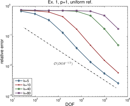
(a) $p=1$

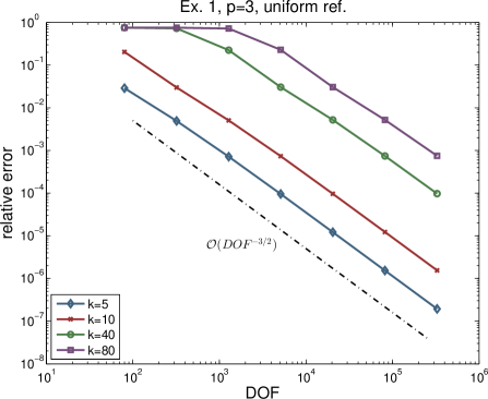
(b) $p=3$

Figure 1: Comparison of the relative error in the norm $\|\cdot\|_{\mathcal{H};\mathcal{T}}$, for the polynomial degrees $p=1$ and $p=3$ for different values of $k$ in Example 1.

Next we test the sharpness of the reliability estimate for the error estimator. In Fig. 2 the ratio $\left\|u-u_{\mathcal{T}}\right\|_{\mathcal{H};\mathcal{T}}/\check{\eta}\left(u_{\mathcal{T}}\right)$ for different polynomial degrees and wavenumbers are depicted. Since we start with a very coarse initial mesh the constant $M_{\frac{\operatorname*{kh}}{\operatorname*{p}}}$ increases with increasing $k$ in the pre-asymptotic regime and, due to Remark 3.8.c, an underestimating can be expected (as compared to when the asymptotic regime is reached). This effect can be seen in Fig. 2 while the asymptotic regime is reached faster for higher order polynomial degree.

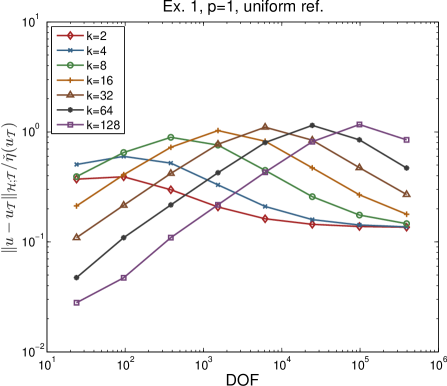
(a) $p=1$

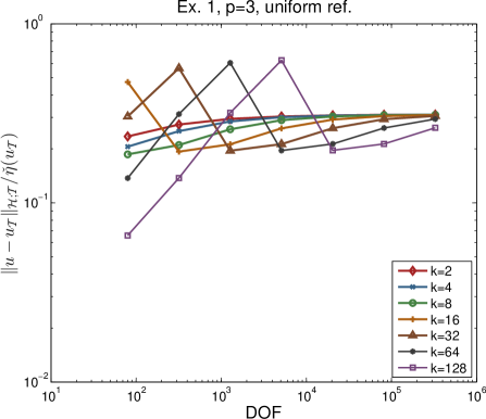
(b) $p=3$

Figure 2: Ratio of the exact error $\|u-u_{\mathcal{T}}\|_{\mathcal{H};\mathcal{T}}$ and the estimated error $\check{\eta}(u_{\mathcal{T}})$ for different values of $k$ in Example 1.

4.2.2 Example 2

We consider the Helmholtz problem on $\Omega=\left(0,2\pi\right)^{2}$ with the exact solution $u\left(x,y\right)=\exp\left(\operatorname*{i}kx\right)$. The corresponding functions $f$ and $g$ are chosen accordingly:

$$f:=0\quad\text{and\quad}g\left(x,y\right):=\left\{\begin{array}[c]{ll}0&\text{if }x=0,\\ 2\operatorname*{i}k&\text{if }x=2\pi,\\ \operatorname*{i}k\operatorname*{e}^{\operatorname*{i}kx}&\text{otherwise,}\end{array}\right.\qquad\forall\left(x,y\right)\in\partial\Omega.$$ (4.1)

The $\operatorname*{dG}$-solution for very coarse meshes is strongly polluted and does not reflect the uniformly oscillating behavior, e.g., in the imaginary part $\operatorname{Im}u=\sin kx$ of the solution. One possible interpretation is that $f=0$ in $\Omega$ and $g=0$ at the left boundary have the effect that $u_{\mathcal{T}}$ is small close to the left boundary while at the right boundary the oscillations got resolved earlier. This is “seen” also by the error estimator and stronger refinement takes place in the early stage of adaptivity close to the right boundary. Only after some refinement steps the strong mesh refinement penetrates from right to left into the whole domain (see. Fig. 3). In Fig. 4(a), we see that the mesh starts to become uniform as soon as the resolution condition (3.27) is fulfilled and the error starts to decrease.

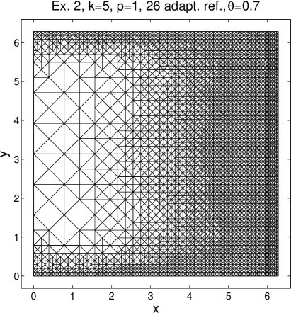
(a) Mesh after 26 adaptive refinements, 9044 elements, $\min_{e}h_{e}=0.049$

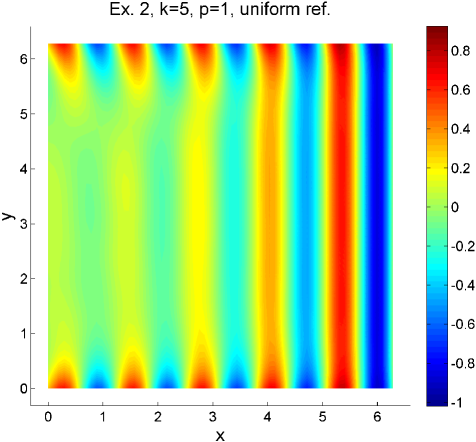
(b) $\Im(u_{\mathcal{T}})$ for a uniformly refined mesh

Figure 3: Adaptive mesh and imaginary part of the DGFEM solution for a uniform mesh with large mesh width, $k=5$, and $p=1$ in Example 2. The exact solution is $u(x,y)=\exp(\operatorname*{i}kx)$, and therefore $\Im(u(x,y))=\sin(kx)$.

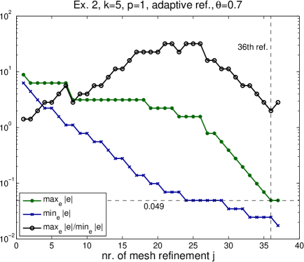
(a) In this plot $|e|$ denotes the length of the edge $e$. The plot shows the maximum length of an edge, the minimum length of an edge, and the ratio for the $j$-th adaptively refined mesh.

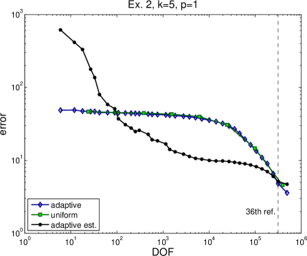
(b) Error $\|u-u_{\mathcal{T}}\|_{\mathcal{H};\mathcal{T}}$ for uniform and adaptive refinement (with $\theta=0.7$) and the estimated error $\check{\eta}(u_{\mathcal{T}})$ for adaptive refinement

Figure 4: In Fig. (a) it can be seen that the adaptive algorithm, applied to Example 2 with $k=5$ and $p=1$, at first generates a mesh with very diverse element sizes, which then turns into an almost uniform mesh at about the 36th refinement. This refinement corresponds to a maximum edge length of $0.049$. In both plots, the dashed line marks this mesh width, respectively the point at which this adaptive refinement takes place. We observe that convergence for uniform refinement starts shortly before this mesh size is reached. Moreover, at this refinement, the error estimator surpasses the actual error in this example, and the error is underestimated in the preasymptotic range.

Furthermore we emphasize the following two points.

1. As is well-known reliability is not a local property and we have here an example where the local error indicator $\check{\eta}_{K}$ differs significantly from the local error in the left part of the domain in the pre-asymptotic regime. In addition, $M_{\frac{\operatorname*{kh}}{\operatorname*{p}}}$ is large and due to Remark 3.8.c the underestimation of the error in this early stage of refinement can be explained. This behavior is illustrated in Fig. 4(b).

2. It is also worth mentioning that we start the adaptive discretization with a very coarse initial mesh where the resolution condition (3.27) is not fulfilled for a moderate constant $C_{0}$. The numerical experiments indicate that the adaptive process behaves robustly for the $\operatorname*{dG}$-formulation already in the pre-asymptotic regime.

4.3 Example 3: L-shaped Domain

In this example we consider the L-shaped domain $\Omega:=\left(-1,1\right)^{2}\backslash\left(\left[0,1\right]\times\left[-1,0\right]\right)$ with right-hand sides $f$ and $g$ chosen such that the first kind Bessel function $u\left(x,y\right):=J_{1/2}\left(kr\right)$ with $r:=\sqrt{x^{2}+y^{2}}$ is the exact solution (see also [26]). The Bessel function and solution $u$ are plotted in Fig. 5. The problem is chosen such that the solution has a singularity at the reentrant corner located at $\mathbf{0}$.

In Fig. 6, two meshes generated by the adaptive procedure are depicted for uniform polynomial degree $p=1$ and wavenumber $k=10$. The oscillating nature of the solution as well as the singular behavior is nicely reflected by the distribution of the mesh cells.

In Fig. 7, we compare uniform with adaptive mesh refinement for different values of $k$ and $p$. As expected the uniform mesh refinement results in suboptimal convergence rates while the optimal convergence rates are preserved by adaptive refinement for the considered polynomial degrees $p=2,4$. In both cases some initial refinement steps are required before the error starts to decrease due to the pollution effect. Again the pollution is significantly reduced for higher polynomial degree.

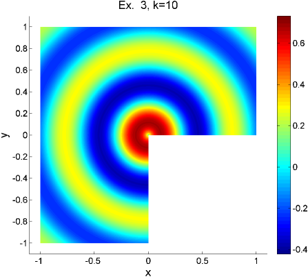
(a) $J_{1/2}(10\|\vec{x}\|)$

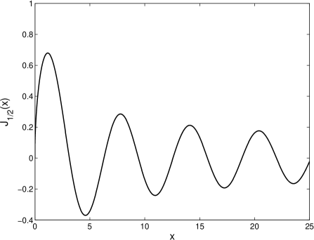
(b) Bessel function $J_{1/2}$ of the first kind

Figure 5: The solution $u=J_{1/2}(kr)$ in Example 3 for $k=10$, and the Bessel function $J_{1/2}(x)$, whose derivative goes to infinity for $x\to 0$.

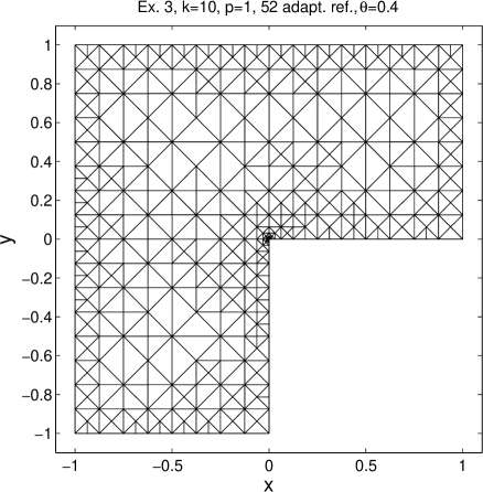
(a) Mesh after 52 refinements, 677 elements, $\min_{e}h_{e}=0.00024$

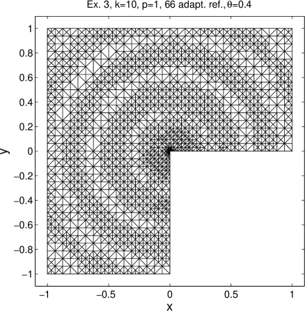
(b) Mesh after 66 refinements, 3677 elements, $\min_{e}h_{e}=0.000022$

Figure 6: Meshes obtained by the adaptive algorithm for Example 3.

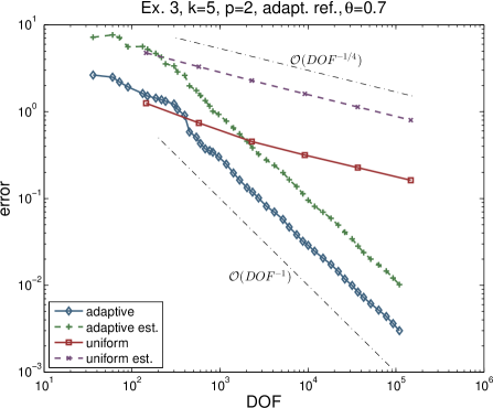
(a) $k=5$, $p=2$

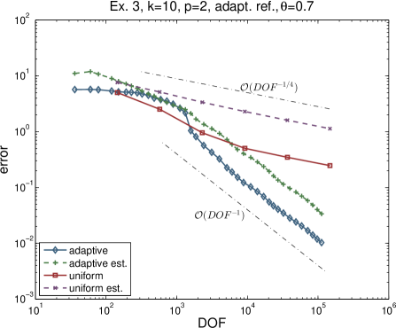
(b) $k=10$, $p=2$

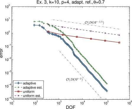
(c) $k=10$, $p=4$

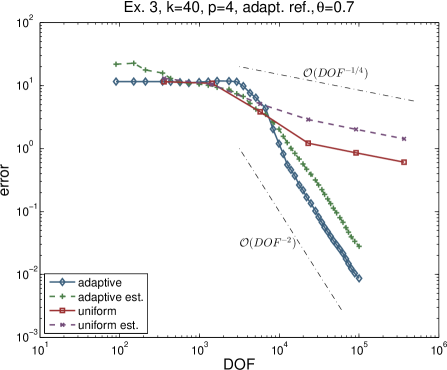
(d) $k=40$, $p=4$

Figure 7: Comparison of the actual error $\|u-u_{\mathcal{T}}\|_{\mathcal{H};\mathcal{T}}$ and the estimated error $\check{\eta}(u_{\mathcal{T}})$, using uniform and adaptive refinement with $\theta=0.7$ in Example 3 for different values of $k$ and $p$.

4.4 Example 4: Non-constant Wavenumber

In this section, we consider the case of non-constant wavenumber $k$ which has important practical applications. Although we have formulated the $\operatorname*{dG}$-method for non-constant wavenumber our theory only covers the constant case. Nonetheless the numerical experiments indicate that the a posteriori error estimation leads to an efficient adaptive solution method.

Consider the domain $\Omega=\left(0,2\pi\right)^{2}$. We partition $\Omega$ into the disc $\Omega_{1}$ about $\left(\pi,\pi\right)^{\top}$ with radius $3/2$ and its complement $\Omega_{2}:=\Omega\backslash\Omega_{1}$. Let $k_{1},k_{2}>0$. The function $k$ is defined piecewise by $\left.k\right|_{\Omega_{i}}:=k_{i}$, $i=1,2$. We have chosen $f=0$ and

$$g_{1}\left(x,y\right):=\left\{\begin{array}[c]{cl}-1&x=0,\\ \operatorname*{i}&x=2\pi,\\ 0&\text{otherwise},\end{array}\right.\qquad\forall\left(x,y\right)\in\partial\Omega.$$ (4.2)

Alternatively we will consider boundary data as defined in (4.1) with $k:=k_{2}$ and denote them here by $g_{2}$.

In Fig. 8, the adaptively refined mesh and the real part of the $\operatorname*{dG}$-solution are plotted for $k_{1}=10$, $k_{2}=1$, and the boundary data $g_{1}$. Strong refinement takes place in the vicinity of the circular interface between $\Omega_{1}$ and $\Omega_{2}$. Moreover, the mesh width is much smaller inside the circle, where the wavenumber is high in accordance with the smoothness properties of the solution.

In the next example we have considered the reversed situation: $k_{1}=1$, $k_{2}=10$, and boundary data $g_{2}$. Fig. 9 implies, that strong refinement close to the jump of the wavenumber is not always necessary. In this case, the solution appears to be smooth, respectively almost zero near the left part of the inner circle where $k=k_{2}$ holds and this is taken into account by the adaptive algorithm. Fig. 10 reflects the convergence of the estimated error for Example 4.

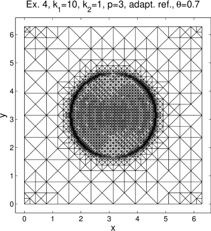
(a) Mesh after 28 refinements, 6076 elements, $\min_{e}h_{e}=0.012$

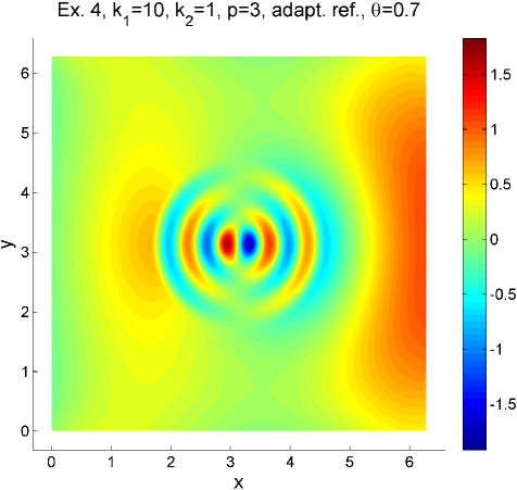
(b) $\Re(u_{\mathcal{T}})$

Figure 8: Adaptively refined mesh with $\theta=0.7$ and real part of the DGFEM solution on this mesh for Example 4 with $k_{1}=10$, $k_{2}=1$, and the boundary data $g_{1}$.

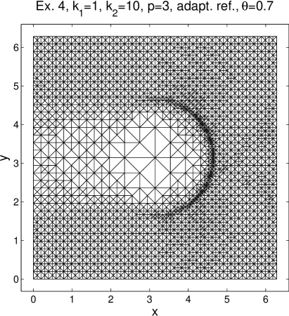
(a) Mesh after 29 refinements, 5892 elements, $\min_{e}h_{e}=0.034$

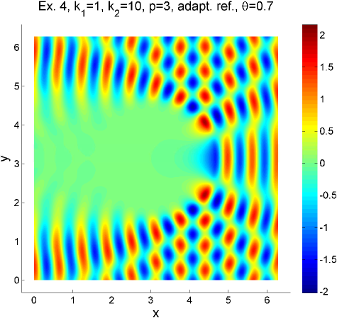
(b) $\Re(u_{\mathcal{T}})$

Figure 9: Adaptively refined mesh with $\theta=0.7$ and real part of the DGFEM solution on this mesh for Example 4 with $k_{1}=1$, $k_{2}=10$, and the boundary data $g_{2}$.

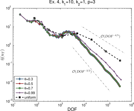
(a) Boundary data $g_{1}$, $k_{1}=10$, $k_{2}=1$

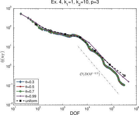
(b) Boundary data $g_{2}$, $k_{1}=1$, $k_{2}=10$

Figure 10: The convergence of the error estimator $\check{\eta}(u_{\mathcal{T}})$ in Example 4 for two non-constant functions $k(x,y)$ and the boundary data $g_{1}$, $g_{2}$, respectively.

These examples indicate that the adaptive algorithm, applied with the error estimator $\check{\eta}_{K}$, properly accomplishes the task of refining the mesh according to the properties of the solution: Singularities and wave characteristics are recognized by the estimator, and we observed optimal convergence rates.

5 Conclusion and Outlook

In this paper we have derived an a posteriori error estimator for an $hp$-$\operatorname*{dG}$ method for highly indefinite Helmholtz problems. In contrast to the discretization of the standard variational formulation of the Helmholtz problem, the chosen $hp$-$\operatorname*{dG}$ discretization always has a unique solution (cf. Remark 2.4). We have proved reliability and efficiency estimates which are explicit in the discretization parameters $h$, $p$, and the wave number $k$. Note that the adjoint approximation property $\sigma_{k}^{\ast}\left(S_{\mathcal{T}}^{\mathfrak{p}}\right)$ enters the reliability estimate. In [47, Thm. 2.4.2] and [37, 36] it has been proved that for convex polygonal domains the conditions

$$p\geq C_{0}\log k\quad\text{and\quad}\forall K\in\mathcal{T}:\quad\frac{kh_{K}}{p_{K}}\leq C_{1}$$ (5.1)

imply $\sigma_{k}^{\ast}\left(S_{\mathcal{T}}^{\mathfrak{p}}\right)\leq C_{2}$. We expect that general polygonal domains can be handled by a) generalizing the “decomposition lemma” [38, Theorem 4.10] to a weighted $H^{2}\left(\Omega\right)$-regularity estimate for the non-analytic part of the adjoint solution and b) performing an appropriate mesh grading towards reentrant corners as is well known for elliptic boundary value problem. Then, the error estimate for the non-analytic part can be derived in a similar fashion as the estimate of $\eta_{\mathcal{A}}$ in the proof of [38, Proposition 5.6]. Again, we expect that the resolution condition (5.1) remains unchanged while the constant $C_{1}$ then, possibly, depends on the angles at the reentrant corners of the polygon. Whereas the rigorous derivation of such estimates is a topic of future research, we point out that the use of adaptive methods is already justified in our model setting of convex polygons, since higher polynomial degrees require graded meshes also at convex corners in order to preserve optimal convergence rates.

Our analysis is not sharp enough to give precise bounds for the constants $C_{0}$, $C_{1}$, $C_{2}$. The numerical experiments show that these estimates are qualitatively sharp, i.e., if the polynomial degree stays fixed independent of $k$, the error estimator significantly overestimates the error while a mild, logarithmic increase depending on $k$ cures this problem. It would be also interesting to estimate the size of $\sigma_{k}^{\ast}\left(S_{\mathcal{T}}^{\mathfrak{p}}\right)$ by numerical experiments. However, this task is far from being trivial because the adjoint approximation property is defined as an infinite-dimensional $\sup$-$\inf$ problem, and the dependence on the regularity of the domain, step size $h$, polynomial degree $p$, wave number $k$ requires extensive numerical tests which would increase the length of the paper substantially. We are planning to investigate this question as a topic of further research. Our numerical examples indicate that, as soon as the resolution condition is satisfied with constants $C_{0}\sim C_{1}=\mathcal{O}\left(1\right)$, the a posteriori error estimator becomes quite sharp.

Another interesting question is related to the mesh grading towards the corners of the polygonal domain. The results in [38] imply that if the initial, coarsest mesh and polynomial degrees are chosen according to (5.1) and [38, Assumption 5.4] then, $\sigma_{k}^{\ast}\left(S_{\mathcal{T}}^{\mathfrak{p}}\right)$ stays bounded by a constant during the whole adaptive process and the geometric grading may not to be incorporated in the adaptive refinement procedure. Our numerical experiments show that after some refinements (as soon as the resolution condition is satisfied) the convergence rate of the adaptive solution becomes optimal and, in addition, the error estimator nicely reflects the size and decay of the error. This behaviour of the estimator, which is supported by our analysis only in case $\sigma_{k}^{\ast}\left(S_{\mathcal{T}}^{\mathfrak{p}}\right)$ that is moderate, suggests that the adaptive algorithm achieves an appropriate mesh grading on its own.

Appendix A Approximation Properties

A.1 $C^{1}$-$hp$ Interpolant

For residual-type a posteriori error estimation, typically, the subtle choice of an interpolation operator for the approximation of the error along $hp$-explicit error estimates plays an essential role. For our non-conforming $\operatorname{dG}$-formulation it turns out that a $C^{1}$-interpolation operator has favorable properties, namely, the internal jumps vanish while the approximation estimates are preserved. In [39] a $C^{0}$-$hp$-Clément-type interpolation operator is constructed and $hp$-explicit error estimates are derived for $W^{1,q}\left(\Omega\right)$ functions. In contrast, our estimate for the $C^{1}$-hp Clément interpolation operator allows for higher-order convergence estimates for smoother functions as well as for estimates in norms which are stronger than the $H^{1}$-norm. The proof follows the ideas in [39, Thm. 2.1] and employs a $C^{1}$-partition of unity by the quintic Argyris finite element.

The construction is in two steps. First local (discontinuous) approximations are constructed on local triangle patches. By multiplying with a $C^{1}$-partition of unity the resulting approximation is in $C^{1}\left(\Omega\right)$, while the approximation properties are preserved.

The first step is described by the following theorem. Its proof can be found in [35, Thm. 5.1] which is a generalization of the one-dimensional construction (see, e.g., [14, Chap. 7, eq. (2.8)]).

Theorem A.1.

Let $d\in\mathbb{N}$ and $I:=\mathop{\mathchoice{\raise-2.20001pt\hbox{\huge$\times$}}{\raise-0.50003pt\hbox{\Large$\times$}}{\hbox{\large$\times$}}{\times}}_{j=1}^{d}I_{j}$ with $I_{i}$ being a bounded interval for every $i\in\left\{1,\ldots,d\right\}$. Let $n\in\mathbb{N}$. Then, for any $p\in\mathbb{N}$ with $p\geq n-1$, there exists a bounded linear operator $J_{n,p}:L^{1}\left(I\right)\rightarrow\bigotimes_{j=1}^{d}\mathbb{P}_{p}\left(I_{j}\right)$ with the following properties: For each $q\in\left[1,\infty\right]$, there exists a constant $C>0$ depending only on $n$, $q$, and $I$ such that for all $0\leq n\leq N$

$$J_{n,p}u =u\qquad\forall u\in{\displaystyle\bigotimes\limits_{j=1}^{d}}\mathbb{P}_{n-1}\left(I_{j}\right)$$

$$\left\|u-J_{n,p}\right\|_{W^{\ell,q}\left(I\right)} \leq C\left(N+1\right)^{-\left(r-\ell\right)}\left|u\right|_{W^{r,q}\left(I\right)},\qquad 0\leq\ell\leq r\leq n.$$

The proof of the following theorem is a generalization of the proof of [39, Thm. 2.1] and is carried out in detail in [47, Thm. 3.1.10]. Here we skip it for brevity.

Theorem A.2 (Clément type quasi-interpolation).

Let $\mathcal{T}$ be a $\rho_{\mathcal{T}}$-shape regular, conforming simplicial finite element mesh for the polygonal Lipschitz domain $\Omega\subseteq\mathbb{R}^{2}$. Let $\mathfrak{p}$ be a polynomial degree function for $\mathcal{T}$ satisfying (2.4). Assume that $q\in\left[1,\infty\right]$ and let $n\in\mathbb{N}$.

1. Assume that $\left\lfloor\left(p_{\mathcal{T}}-5\right)/2\right\rfloor\geq n-1$. Then, there exists a bounded linear operator $I_{n}^{\operatorname{hp}}:W^{n,q}\left(\Omega\right)\rightarrow S_{\mathcal{T}}^{\mathfrak{p}}\cap C^{1}\left(\Omega\right)$ such that for every $K\in\mathcal{T}$

   $$\left|u-I_{n}^{\operatorname{hp}}u\right|_{W^{m,q}\left(K\right)}\leq C\left(\frac{h_{K}}{p_{K}}\right)^{n-m}\left|u\right|_{W^{n,q}\left(\omega_{K}\right)}\qquad\forall m\in\left\{0,\ldots,n\right\},$$ (A.1a)

   and for every $e\in\mathcal{E}\left(K\right)$ and multiindex $\vartheta\in\mathbb{N}_{0}^{2}$ with $\vartheta_{1}+\vartheta_{2}=m\leq n-1$

   $$\left\|\frac{\partial^{m}}{\partial x^{\vartheta_{1}}\partial y^{\vartheta_{2}}}\left(\left.\left(u-I_{n}^{\operatorname{hp}}u\right)\right|_{K}\right)\right\|_{L^{q}\left(e\right)}\leq C\left(\frac{h_{e}}{p_{e}}\right)^{n-m-1/q}\left|u\right|_{W^{n,q}\left(\omega_{e}\right)},$$ (A.1b)

   where $C>0$ only depends on $n$, $q$, $\rho_{\mathcal{T}}$, and $\Omega$.

2. Assume that $\left\lfloor\left(p_{\mathcal{T}}-1\right)/2\right\rfloor\geq n-1$. Then, there exists a bounded linear operator $I_{n}^{\operatorname{hp},0}:W^{n,q}\left(\Omega\right)\rightarrow S_{\mathcal{T}}^{\mathfrak{p}}\cap C^{0}\left(\Omega\right)$ such that (A.1) holds with $I_{n}^{\operatorname{hp}}u$ replaced by $I_{n}^{\operatorname{hp},0}u$ for a constant $C>0$ solely depending on $n$, $q$, $\rho_{\mathcal{T}}$, and $\Omega$.

A.2 Conforming Approximation

The a posteriori error analysis for our non-conforming $\operatorname{dG}$-formulation requires the construction of conforming approximants of non-conforming $hp$-finite element functions and this will be provided next.

Theorem A.3 (Conforming approximant).

Let $\mathcal{T}$ be a $\rho_{\mathcal{T}}$-shape regular, conforming simplicial finite element mesh of the polygonal domain $\Omega\subseteq\mathbb{R}^{2}$. Let $v\in S_{\mathcal{T}}^{\mathfrak{p}}$, and let $\mathfrak{p}$ be a polynomial degree function satisfying (2.4) and $p_{\mathcal{T}}\geq 1$. Then, there exists a constant $C>0$ which only depends on the shape regularity and a function $v^{\ast}\in S_{\mathcal{T}}^{\mathfrak{p}}\cap C^{0}\left(\Omega\right)$ such that

$$\left\|v-v^{\ast}\right\|_{\partial\Omega} \leq C\left\|[\![v]\!]\right\|_{\mathfrak{S}^{I}},$$ (A.2a)

$$\left\|v-v^{\ast}\right\| \leq C\left\|\mathfrak{h}^{1/2}[\![v]\!]\right\|_{\mathfrak{S}^{I}},$$ (A.2b)

$$\left\|\nabla\left(v-v^{\ast}\right)\right\| \leq C\left\|\frac{\mathfrak{p}}{\mathfrak{h}^{1/2}}[\![v]\!]\right\|_{\mathfrak{S}^{I}}.$$ (A.2c)

For the proof of this theorem we refer to [47, Thm. 3.2.7] (see also, e.g., [27, 7]).

Corollary A.4 (Conforming error).

Let the assumptions of Theorem A.3 be satisfied. There exists a constant $C>0$ which only depends on the shape regularity constant $\rho_{\mathcal{T}}$ such that, for every $v\in S_{\mathcal{T}}^{p}$, there is a function $v^{\ast}\in S_{\mathcal{T}}^{\mathfrak{p}}\cap C^{0}\left(\Omega\right)$ with

$$\left\|k\left(v-v^{\ast}\right)\right\|^{2}+\left\|\nabla\left(v-v^{\ast}\right)\right\|^{2}+ \left\|\sqrt{k}\left(v-v^{\ast}\right)\right\|_{\partial\Omega}^{2}$$

$$\leq\frac{C}{\mathfrak{a}}\left(1+\frac{1}{p_{\mathcal{T}}}M_{\frac{\operatorname*{kh}}{\operatorname*{p}}}+M_{\frac{\operatorname*{kh}}{\operatorname*{p}}}^{2}\right)\left\|\sqrt{{\mathfrak{a}\frac{\mathfrak{p}^{2}}{\mathfrak{h}}}}[\![v]\!]\right\|_{\mathfrak{S}^{I}}^{2}.$$

Proof.

The estimate follows by (A.2).   ∎

References

- [1] J. D. Achenbach. Wave propagation in elastic solids. North Holland, Amsterdam, 2005.
- [2] M. Ainsworth and J. T. Oden. A Posteriori Error Estimation in Finite Element Analysis. Wiley, 2000.
- [3] I. Babuška, F. Ihlenburg, T. Strouboulis, and S. K. Gangaraj. A posteriori error estimation for finite element solutions of Helmholtz’ equation I. The quality of local indicators and estimators. Internat. J. Numer. Methods Engrg., 40(18):3443–3462, 1997.
- [4] I. Babuška, F. Ihlenburg, T. Strouboulis, and S. K. Gangaraj. A posteriori error estimation for finite element solutions of Helmholtz’ equation II. Estimation of the pollution error. Internat. J. Numer. Methods Engrg., 40(21):3883–3900, 1997.
- [5] I. Babuška and W. C. Rheinboldt. A-posteriori error estimates for the finite element method. Internat. J. Numer. Meth. Engrg., 12:1597–1615, 1978.
- [6] I. Babuška and W. C. Rheinboldt. Error estimates for adaptive finite element computations. SIAM J. Numer. Anal., 15:736–754, 1978.
- [7] A. Bonito and R. H. Nochetto. Quasi-optimal convergence rate of an adaptive discontinuous Galerkin method. SIAM J. Numer. Anal., 48(2):734–771, 2010.
- [8] A. Buffa and P. Monk. Error estimates for the ultra weak variational formulation of the Helmholtz equation. M2AN Math. Model. Numer. Anal., 42(6):925–940, 2008.
- [9] O. Cessenat and B. Després. Application of an ultra weak variational formulation of elliptic PDEs to the two-dimensional Helmholtz equation. SIAM J. Numer. Anal., 35:255–299, 1998.
- [10] O. Cessenat and B. Després. Using plane waves as base functions for solving time harmonic equations with the ultra weak variational formulation. J. Computational Acoustics, 11:227–238, 2003.
- [11] S. N. Chandler-Wilde, I. G. Graham, S. Langdon, and E. A. Spence. Numerical-asymptotic boundary integral methods in high-frequency acoustic scattering. Acta Numer., 21:89–305, 2012.
- [12] P. Cummings and X. Feng. Sharp regularity coefficient estimates for complex-valued acoustic and elastic Helmholtz equations. Math. Models Methods Appl. Sci., 16(1):139–160, 2006.
- [13] B. Després. Sur une formulation variationnelle de type ultra-faible. C. R. Acad. Sci. Paris Sér. I Math., 318(10):939–944, 1994.
- [14] R. A. DeVore and G. G. Lorentz. Constructive Approximation. Springer-Verlag, New York, 1993.
- [15] D. A. Di Pietro and A. Ern. Mathematical aspects of discontinuous Galerkin methods. Springer, Heidelberg, 2012.
- [16] W. Dörfler and S. Sauter. A posteriori error estimation for highly indefinite Helmholtz problems. Comput. Methods Appl. Math., 13(3):333–347, 2013.
- [17] S. Esterhazy and J. M. Melenk. On stability of discretizations of the Helmholtz equation. In I. Graham, T. Hou, O. Lakkis, and R. Scheichl, editors, Numerical Analysis of Multiscale Problems, volume 83 of Lect. Notes Comput. Sci. Eng., pages 285–324. Springer, Berlin, 2012.
- [18] X. Feng and H. Wu. Discontinuous Galerkin methods for the Helmholtz equation with large wave number. SIAM J. Numer. Anal., 47(4):2872–2896, 2009.
- [19] X. Feng and H. Wu. -discontinuous Galerkin methods for the Helmholtz equation with large wave number. Math. Comp., 80(276):1997–2024, 2011.
- [20] X. Feng and Y. Xing. Absolutely stable local discontinuous Galerkin methods for the Helmholtz equation with large wave number. Math. Comp., 82(283):1269–1296, 2013.
- [21] C. Gittelson, R. Hiptmair, and I. Perugia. Plane wave discontinuous Galerkin methods: Analysis of the h-version. Int. J. Numer. Meth. Engr., 43(2):297–331, 2009.
- [22] M. Grigoroscuta-Strugaru, M. Amara, H. Calandra, and R. Djellouli. A modified discontinuous Galerkin method for solving efficiently Helmholtz problems. Commun. Comput. Phys., 11(2):335–350, 2012.
- [23] I. Harari. A survey of finite element methods for time-harmonic acoustics. Comput. Methods Appl. Mech. Engrg., 195(13-16):1594–1607, 2006.
- [24] I. Harari and T. J. R. Hughes. Galerkin/least-squares finite element methods for the reduced wave equation with nonreflecting boundary conditions in unbounded domains. Comput. Methods Appl. Mech. Engrg., 98(3):411–454, 1992.
- [25] R. Hiptmair, A. Moiola, and I. Perugia. Plane wave discontinuous Galerkin methods for the 2D Helmholtz equation: analysis of the -version. SIAM J. Numer. Anal., 49(1):264–284, 2011.
- [26] R. H. W. Hoppe and N. Sharma. Convergence analysis of an adaptive interior penalty discontinuous Galerkin method for the Helmholtz equation. IMA J. Numer. Anal., 33(3):898–921, 2013.
- [27] P. Houston, D. Schötzau, and T. P. Wihler. Energy norm a posteriori error estimation of -adaptive discontinuous Galerkin methods for elliptic problems. Math. Models Methods Appl. Sci., 17(1):33–62, 2007.
- [28] T. Huttunen and P. Monk. The use of plane waves to approximate wave propagation in anisotropic media. J. Computational Mathematics, 25:350–367, 2007.
- [29] F. Ihlenburg. Finite Element Analysis of Acousting Scattering. Springer, New York, 1998.
- [30] F. Ihlenburg and I. Babuška. Finite Element Solution to the Helmholtz Equation with High Wave Number. Part II: The h-p version of the FEM. SIAM J. Num. Anal., 34(1):315–358, 1997.
- [31] S. Irimie and P. Bouillard. A residual a posteriori error estimator for the finite element solution of the Helmholtz equation. Comput. Methods Appl. Mech. Engrg., 190(31):4027–4042, 2001.
- [32] J. D. Jackson. Classical electrodynamics. John Wiley & Sons, Inc., New York-London-Sydney, second edition, 1975.
- [33] R. Kellogg. Interpolation between subspaces of a Hilbert space. Technical Report BN-719, Institute for Fluid Dynamics and Applied Mathematics, University of Maryland at College Park, College Park, MD, 20742-2431,USA, 1971.
- [34] J. M. Melenk. On Generalized Finite Element Methods. PhD thesis, University of Maryland at College Park, 1995.
- [35] J. M. Melenk. -interpolation of nonsmooth functions and an application to -a posteriori error estimation. SIAM J. Numer. Anal., 43(1):127–155, 2005.
- [36] J. M. Melenk, A. Parsania, and S. Sauter. Generalized DG Methods for Highly Indefinite Helmholtz Problems Based on the Ultra-Weak Variational Formulation. J Sci Comput, 57:536–581, 2013.
- [37] J. M. Melenk and S. Sauter. Convergence Analysis for Finite Element Discretizations of the Helmholtz equation with Dirichlet-to-Neumann boundary condition. Math. Comp, 79:1871–1914, 2010.
- [38] J. M. Melenk and S. Sauter. Wave-Number Explicit Convergence Analysis for Galerkin Discretizations of the Helmholtz Equation. SIAM J. Numer. Anal., 49(3):1210–1243, 2011.
- [39] J. M. Melenk and B. I. Wohlmuth. On residual-based a posteriori error estimation in -FEM. Adv. Comput. Math., 15(1-4):311–331 (2002), 2001.
- [40] P. Monk and D.-Q. Wang. A least-squares method for the Helmholtz equation. Comput. Methods Appl. Mech. Engrg., 175(1-2):121–136, 1999.
- [41] R. H. Nochetto, K. G. Siebert, and A. Veeser. Theory of adaptive finite element methods: an introduction. In Multiscale, nonlinear and adaptive approximation, pages 409–542. Springer, Berlin, 2009.
- [42] J. T. Oden, S. Prudhomme, and L. Demkowicz. A posteriori error estimation for acoustic wave propagation problems. Arch. Comput. Methods Engrg., 12(4):343–389, 2005.
- [43] A. H. Schatz. An observation concerning Ritz-Galerkin methods with indefinite bilinear forms. Math. Comp., 28:959–962, 1974.
- [44] C. Schwab. - and -finite element methods. The Clarendon Press Oxford University Press, New York, 1998.
- [45] R. Verfürth. A posteriori error estimation techniques for finite element methods. Oxford University Press, Oxford, 2013.
- [46] H. Wu. Pre-asymptotic error analysis of cip-fem and fem for the helmholtz equation with high wave number. part i: linear version. IMA Journal of Numerical Analysis, 2013.
- [47] J. Zech. A Posteriori Error Estimation of -DG Finite Element Methods for Highly Indefinite Helmholtz Problems. Master’s thesis, Inst. f. Mathematik, Unversität Zürich, 2014. https://www.math.uzh.ch/compmath/index.php?id=zech.
- [48] L. Zhu and H. Wu. Preasymptotic error analysis of CIP-FEM and FEM for Helmholtz equation with high wave number. Part II: version. SIAM J. Numer. Anal., 51(3):1828–1852, 2013.